Distinguishing Dirac and Majorana Heavy Neutrinos
at Lepton Colliders

Abstract

We discuss the potential to observe lepton number violation (LNV) in displaced vertex searches for heavy neutral leptons (HNLs) at future lepton colliders. Even though a direct detection of LNV is impossible for the dominant production channel because lepton number is carried away by an unobservable neutrino, there are several signatures of LNV that can be searched for. They include the angular distribution and spectrum of decay products as well as the HNL lifetime. We comment on the perspectives to observe LNV in realistic neutrino mass models and argue that the dichotomy of Dirac vs Majorana HNLs is in general not sufficient to effectively capture their phenomenology, but these extreme cases nevertheless represent well-defined benchmarks for experimental searches. Finally, we present accurate analytic estimates for the number of events and sensitivity regions during the $Z$-pole run for both Majorana and Dirac HNLs.

1 Motivation

Neutrinos are the sole fermions in the Standard Model of particle physics (SM) that could be their own antiparticles, in which case the would be the only known elementary Majorana fermions, and their masses would break the global $U(1)_{B-L}$ symmetry of the SM. An immediate consequence would be the existence of processes that violate the total lepton number $L$. However, due to the smallness of the light neutrino masses $m_{i}$ the rate for lepton number violating (LNV) processes in neutrino experiments would be parametrically suppressed. At the same time it is clear that any explanation of the light neutrino masses requires an extension of the SM field content, and LNV may occur at an observable rate in processes involving new particles. This in particular can include heavy neutral leptons (HNLs) $N_{i}$ that couple to the $Z$- and $W$-bosons and the Higgs bosons $h$ via the SM weak interaction with an amplitude suppressed by the mixing angles $\theta_{\alpha i}$ (with $\alpha=e,\mu,\tau$ and $i=1\ldots n$),

$$\mathcal{L}\supset-\frac{m_{W}}{v}\overline{N}_{i}\theta^{*}_{\alpha i}\gamma^{\mu}e_{L\alpha}W^{+}_{\mu}-\frac{m_{Z}}{\sqrt{2}v}\overline{N}_{i}\theta^{*}_{\alpha i}\gamma^{\mu}\nu_{L\alpha}Z_{\mu}-\frac{M_{i}}{v\sqrt{2}}\theta_{\alpha i}h\overline{\nu_{L}}_{\alpha}N_{i}+\text{h.c.},$$ (1)

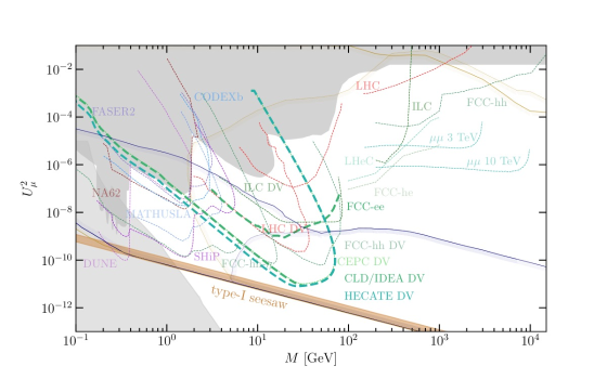
(a)

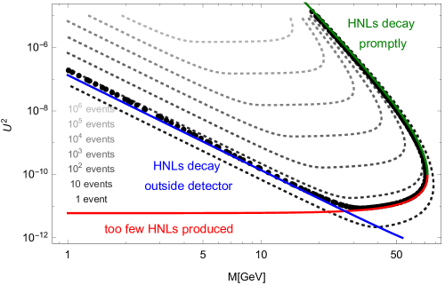
(b)

Figure 1: (a) Allowed HNL parameter region (white) compared to the sensitivities of various experiments, in particular displaced vertex searches at FCC-ee and CEPC, details given in [49]. (b) Simulated 4-event curves from [49] (black dots) compared to the analytic estimates (2) (gray dotted), (8a) (red) (8b) (green) and (9) (blue) for $U^{2}=U_{\mu}^{2}$, $c_{\rm prod}=c_{\rm dec}=1$, $N_{\text{obs}}=4$, $N_{\rm IP}=2$, $N_{Z}=2.5\times 10^{12}$, $l_{0}=400\mu$m, $d_{\rm cyl}=10$m, $l_{\rm cyl}=8.6$m, $\epsilon_{\alpha\beta}=1$.Public codes to estimate the number of events and sensitivity regions based on the analytic approximations (2), (8a), (8b) and (9) are made available at [50].

with $m_{Z}$, $m_{W}$ the weak gauge boson masses and $v\simeq 174$ GeV the Higgs field vacuum expectation value. The $N_{i}$ can be Dirac or Majorana fermions. For $M_{i}<m_{Z}$ they can be produced copiously during the $Z$-pole run of future lepton colliders [19] such as FCC-ee [20] or CEPC [21], cf. Fig. 1(a), making it possible to not only discover them but also study their properties in sufficient detail to probe their role in neutrino mass generation and leptogenesis [25]. An important question in this context is whether the LNV in $N_{i}$-decays can be observed. This is hampered by two main obstacles, both of which can be overcome,

• LNV can be detected most directly when the final state of a process can be fully reconstructed, such as $W^{\pm}\to\ell_{\alpha}^{\pm}N\to\ell_{\alpha}^{\pm}\ell^{\pm}_{\alpha}W^{\mp}_{*}$. However, at lepton colliders $N_{i}$ with $M_{i}<m_{Z}$ are dominantly produced in the decays of $Z$-bosons along with an unobservable neutrino or antineutrino, making it impossible to reconstruct the final state and determine its total $L$.

• In models that employ the type-I seesaw mechanism [26, 27, 28, 29, 30, 31], the light neutrino masses parametrically scale as $m_{i}\sim\theta^{2}M_{i}$, while the HNL production cross section scales as $\sigma_{N}\sim\theta^{2}$, cf. (2), so that one may expect $\sigma_{N}$ to be parametrically suppressed by $\sim m_{i}/M_{i}$. This is not the case if the $m_{i}$ are protected by an approximate global $U(1)_{B-\bar{L}}$ symmetry, with $\bar{L}$ a generalised lepton-number under which the HNLs are charged [33]. The symmetry would lead to systematic cancellations in the neutrino mass matrix that keep the $m_{i}$ small while allowing for (almost) arbitrarily large

  $$U_{\alpha i}^{2}=|\theta_{\alpha i}|^{2}.$$

  The approximate $\bar{L}$-conservation would, however, also suppress all LNV processes parametrically. One may expect that the ratio of $L$-violating to $L$-conserving $N_{i}$-decays scales as $R_{ll}\sim U_{i}^{-2}m_{i}/M_{i}$ with $U_{i}^{2}=\sum_{\alpha}U_{\alpha i}^{2}$ and is practically unobservable even if the $N_{i}$ are fundamentally Majorana particles.

2 Observables sensitive to LNV

Collider studies are often performed in a phenomenological type I seesaw model, defined by (1) with only one HNL species ($n=1$) of mass $M$. This is not a realistic model of neutrino mass, but it can effectively capture many phenomenological aspects with only five parameters $(M,\theta_{e},\theta_{\mu},\theta_{\tau},R_{ll})$, where $R_{ll}=0$ for Dirac-$N$ and $R_{ll}=1$ for Majorana-$N$. If all HNLs decay inside the detector the total number of events with $n=1$ is the same for the Dirac and Majorana cases, but there are at least three ways in which Dirac and Majorana HNLs can be distinguished at FCC-ee.

• In the Dirac case a $N$ ($\bar{N}$) is always produced along with a $\bar{\nu}$ ($\nu$). The chiral nature of the weak interaction and angular momentum conservation imply that $\nu$ and $\bar{\nu}$ are emitted with different angular distributions for a given $Z$-polarisation. Due to the parity-violation of the weak SM interaction the $Z$-bosons at lepton colliders are polarised at the level of $P_{Z}\simeq 15\%$ even if the $e^{\pm}$ beams are not, hence the angular distributions of the $N$ and $\bar{N}$ are different [38]. Since Dirac $N$ ($\bar{N}$) can only decay into leptons (antileptons), this introduces differences in the angular distribution of leptons and antileptons. This can be observed in the form of a forward-backward asymmetry $A_{FB}^{D}\simeq P_{Z}\frac{3}{4}/(1-(M/m_{Z})^{2}/2)\sim 10\%$, cf. Fig. 2(a). For Majorana HNLs there is no forward-backward asymmetry because they can decay into leptons and antileptons.

• For the Dirac case, the $N$ and $\bar{N}$ individually are highly polarised, cf. Fig. 2(b), because $N$ ($\bar{N}$) can only have been produced along with $\bar{\nu}$ ($\nu$), whose helicity is fixed in the massless limit. Since $N$ can only decay into leptonic final states ($\bar{N}$ into antileptonic ones), the parent particle of leptons and antileptons tend to have opposite polarisation. The decay rates are polarisation-dependent [37], leading to different spectra for leptons and antileptons [38]. For Majorana HNL there is no difference between $N$ and $\bar{N}$; their polarisaion is of order (and proportional to) $P_{Z}$, and they can decay into either leptons and antileptons. This difference in the lepton spectra is observable.

• For long-lived HNLs counting the number of events as a function of displacement provides an additional probe that is independent of $P_{Z}$. While the number $N_{{\rm HNL}\alpha}$ of HNLs produced in $Z$-decays along with a lepton or antilepton of flavour $\alpha$ is the same for Dirac and Majorana HNLs, their decay rate differs by a factor two, leading to a twice larger decay length in the detector $\lambda_{N}=\upbeta\upgamma/\Gamma_{N}$, with $\upbeta\upgamma={\rm p}_{N}/M$ and ${\rm p}_{N}$ the HNL three-momentum. Hence, the number of HNL decays into lepton flavour $\beta$ with a displacement between $l_{0}$ and $l_{1}$ is sensitive to this difference. It is given by

  $$N_{\text{obs}}\simeq\ratio{\beta}N_{{\rm HNL}\alpha}\left[\exp(-l_{0}/\lambda_{N})-\exp(-l_{1}/\lambda_{N})\right]\epsilon_{\alpha\beta},$$ (2)

  with $0\leq\epsilon_{\alpha\beta}\leq 1$ an overall efficiency factor. Here

  $$\ratio{\alpha}=\frac{U_{\alpha}^{2}}{U^{2}}$$

  and [41, 48]

  $$N_{{\rm HNL}\alpha}\simeq 2\ratio{\alpha}U^{2}c_{\rm prod}N_{Z}N_{\rm IP}{\rm B}^{Z}_{\alpha}\Pi$$

  where

  $$\Pi=\left(\frac{2{\rm p}_{N}}{m_{Z}}\right)^{2}\left(1+\frac{(M/m_{Z})^{2}}{2}\right)\ ,\ {\rm p}_{N}=\frac{m_{Z}}{2}\left(1-(M/m_{Z})^{2}\right),$$

  ${\rm B}^{Z}_{\alpha}=\operatorname{BR}(Z\mathpunct{\to}\nu_{\alpha}\overline{\nu}_{\alpha})=\frac{1}{5}\frac{1}{3}$, $\upbeta\upgamma={\rm p}_{N}/M$, $N_{\rm IP}$ and $N_{Z}$ the number of interaction points and number of $Z$-bosons produced at each of them, and $c_{\rm prod}$ a numerical coefficient that is the same for Dirac or Majorana HNL ($c_{\rm prod}=1$) if $n=1$. The decay rate is [41]

  $$\Gamma_{N}\simeq c_{\rm dec}\frac{a}{96\pi^{3}}U^{2}M^{5}G_{F}^{2}$$

  with $a\simeq 12$ for $M<m_{Z}$ with $c_{\rm dec}=1$ ($c_{\rm dec}=1/2$) for Majorana (Dirac), and

  $$\lambda_{N}=\frac{\upbeta\upgamma}{\Gamma_{N}}\simeq\frac{1.6}{U^{2}c_{\rm dec}}\left(\frac{M}{\rm GeV}\right)^{-6}\left(1-(M/m_{Z})^{2}\right){\rm cm}.$$

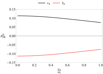
(a)

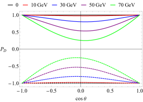
(b)

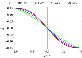
(c)

Figure 2: (a): Forward-backward asymmetry as a function of $M/m_{Z}$. (b) and (c): Polarisations of Dirac ($P_{D}$) and Majorana ($P_{M}$) HNLs as a function of the electron-HNL angle. Plots from [38].

3 Probing realistic neutrino mass models and leptogenesis

Realistic neutrino mass models typically require more than one HNL flavour. In the type-I seesaw $n$ must equal or exceed the number of non-zero $m_{i}$. In technically natural low-scale realisations that can be probed at colliders the $m_{i}$ are protected by a symmetry, cf issue II). If the symmetry is exact, the HNLs have to be organised in pairs with [52]

$$M_{i}=M_{j}\ {\rm and}\ \theta_{\alpha i}={\rm i}\theta_{\alpha j}$$

that form Dirac spinors with distinctively different $N$ and $\bar{N}$; this would imply $m_{i}=0$ and $R_{ll}=0$. Naively one would expect that the tiny symmetry breaking due to the $m_{i}\neq 0$ can only lead to an unobservably small $R_{ll}$, cf. issue II). However, even a small splitting $\Delta M$ between the physical HNL masses induced by the symmetry breaking can give rise to $\bar{L}$-violating oscillations between the $N$-like and $\bar{N}$-like states inside the detector (cf. [53, 54] and references therein). If the HNL decay length $\lambda_{N}$ exceeds the oscillation length, LNV processes are unsuppressed. Since $\Delta M\ll M_{i}$ for the approximate symmetry to protect the $m_{i}$, $\Delta M$ may be smaller than the experimental mass resolution $\delta M_{\rm exp}$, resulting in a single resonance that is effectively characterised by a non-integer [55]

$$R_{ll}=\frac{\Delta M^{2}}{2\Gamma_{N}^{2}+\Delta M^{2}}.$$

Figure 3(a) shows what values of $R_{ll}$ one can expect as a function of $M$ and $U^{2}$ [56], indicating that LNV would be observable in long-lived HNL searches at lepton colliders. For $\Delta M/\Gamma_{N}\sim\ {\rm a\ few}$, it may further be possible to resolve the HNL oscillations by observing $R_{ll}$ as a function of the displacement [57], cf. Fig 3(b).

In summary, the phenomenology of realistic seesaw models is much richer than that of the widely-used phenomenological model (1) with $n=1$. Effectively many aspects can effectively still be captured in this model by adjusting $R_{ll}$, $c_{\rm dec}$, $c_{\rm prod}$ to non-integer values, and if one considers $R_{ll}$ as a function of the displacement. The extreme cases $R_{ll}=1$ and $R_{ll}=0$ are realised in the lower left and upper right corner of Fig. 3(a), respectively. They represent well-defined benchmarks [45] that can easily be implemented in event generators, but it is important to keep in mind that nature is likely to be more complex.

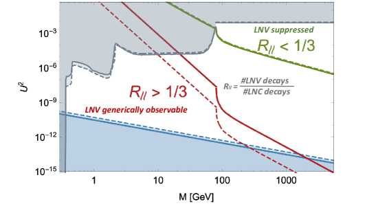
(a)

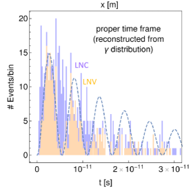
(b)

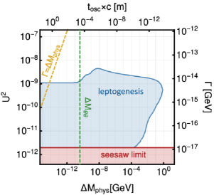
(c)

Figure 3: (a): Parameter region where $R_{ll}$ is suppressed or not [56], (b) and (c): reconstructed HNL oscillation time at LHCb [57] (will be easier at FCC-ee because of the smaller boost) compared to the oscillation time expected from leptogenesis [25].

4 Practical feasibility and number of events

Discovering HNLs only requires a handful of events, but studying their properties with the methods 1)-3) (or others) will require reliable statistics. In displaced vertex searches the number of events can vary by many orders of magnitude across the sensitivity region. For the $Z$-pole run at FCC-ee or CEPC we can reliably estimate the total number of observed HNL decays inside a cylindrical detector of length $l_{\rm cyl}$ and diameter $d_{\rm cyl}$ by identifying $l_{0}$ in (2) with the smallest displacement for which the assumption of vanishing backgrounds can be justified and setting

$$l_{1}=\frac{1}{2}(3/2)^{1/3}d_{\rm cyl}^{2/3}l_{\rm cyl}^{1/3}$$

so that a sphere of radius $l_{1}$ has the same volume as the cylinder, cf. Fig. 15. In the limit of an infinitely large detector we can estimate the maximal mixing $U^{2}_{\rm max}$ and the minimal mixing $U^{2}_{\rm min}$ for which one can see $N_{\rm obs}$ events by solving (2) with $l_{1}\to\infty$ for $U^{2}$,

$$U^{2}_{\rm min} =\frac{W_{0}\left(XY\right)}{X}\simeq Y$$ (8a)

$$U^{2}_{\rm max} =\frac{W_{-1}\left(XY\right)}{X}\simeq\frac{\log\left(-XY\right)}{X}$$ (8b)

where

$$X=-\frac{l_{0}}{U_{\beta}^{2}\lambda_{N}}=-\frac{aG_{F}^{2}l_{0}M^{6}c_{\rm dec}}{96{\rm p}_{N}\pi^{3}}\ ,\quad Y=\frac{U^{2}N_{\rm obs}/\ratio{\beta}}{\epsilon_{\alpha\beta}N_{{\rm HNL}\alpha}}=\frac{N_{\text{obs}}/(\ratio{\alpha}\ratio{\beta})}{2\epsilon_{\alpha\beta}{\rm B}^{Z}_{\alpha}c_{\rm prod}N_{\rm IP}\Pi N_{Z}},$$

with $W_{s}$ the $s$-branch of the Lambert W-function. For $U^{2}>U^{2}_{\rm max}$ for assumption of background-freedom is not justified. For $U^{2}<U^{2}_{\rm min}$ less than $N_{\rm obs}$ HNLs are produced in the first place, so even an infinitely large ideal detector could not see enough decays. Both limits strongly depend on $M$. The finite detector size comes into play for very long-lived HNLs, for which one can expand the exponential in (2) and find (neglecting $l_{0}$)

$$U_{\rm min}^{2}=\frac{2^{1/6}3^{1/3}8\pi^{3/2}({\rm p}_{N}Y)^{1/2}}{(ac_{\rm dec})^{1/2}G_{F}M^{3}d_{\rm cyl}^{1/3}l_{\rm cyl}^{1/6}}\simeq\sqrt{\frac{N_{\text{obs}}}{\ratio{\alpha}\ratio{\beta}}}\frac{57}{G_{F}M^{3}}\sqrt{{\rm p}_{N}}d_{\rm cyl}^{-1/3}l_{\rm cyl}^{-1/6}\left(\epsilon_{\alpha\beta}N_{Z}N_{\rm IP}c_{\rm dec}c_{\rm prod}\Pi\right)^{-1/2}$$ (9)

The dependence of (9) on $l_{\rm cyl}$ and $d_{\rm cyl}$ quantifies the sensitivity gain with additional detectors [69, 70]. The smallest mixing that can be probed is given by the maximum of $U_{\rm min}^{2}$ in (8a) and (9); one can estimate the point where they cross at

$$M\simeq\frac{2.75}{G_{F}^{1/3}d_{\rm cyl}^{1/9}l_{\rm cyl}^{1/18}}\left(\frac{{\rm B}^{Z}_{\alpha}c_{\rm prod}N_{Z}m_{Z}N_{\rm IP}}{c_{\rm dec}N_{\text{obs}}/(\ratio{\alpha}\ratio{\beta})}\right)^{1/6}\simeq\lim_{M/m_{Z}\to 0}2.75\left(\frac{{\rm p}_{N}}{YG_{F}^{2}c_{\rm dec}d_{\rm cyl}^{2/3}l_{\rm cyl}^{1/3}}\right)^{1/6}.$$

Since $N_{{\rm HNL}\alpha}\propto U^{2}$ one can potentially see over a million events at FCC-ee or CEPC, cf. Fig. 15. This does not only make the methods 1)-3) to search for LNV feasible, but also allows for further measurements of the HNL properties, including measurements of $R_{ll}$ and of the $\ratio{\alpha}$. The sensitivity gain that can be achieved with additional detectors [69] can be estimated with (9). This shows the potential of lepton collider to test neutrino mass models and leptogenesis [25].

References

- [1] J. Schechter and J. W. F. Valle, Neutrinoless Double beta Decay in SU(2) x U(1) Theories, Phys. Rev. D 25 (1982) 2951.
- [2] M. Duerr, M. Lindner and A. Merle, On the Quantitative Impact of the Schechter-Valle Theorem, JHEP 06 (2011) 091, [1105.0901].
- [3] W. Rodejohann, Neutrino-less Double Beta Decay and Particle Physics, Int. J. Mod. Phys. E 20 (2011) 1833–1930, [1106.1334].
- [4] A. M. Abdullahi et al., The Present and Future Status of Heavy Neutral Leptons, in 2022 Snowmass Summer Study, 3, 2022. 2203.08039.
- [5] M. Drewes, The Phenomenology of Right Handed Neutrinos, Int. J. Mod. Phys. E 22 (2013) 1330019, [1303.6912].
- [6] M. Fukugita and T. Yanagida, Baryogenesis Without Grand Unification, Phys. Lett. B 174 (1986) 45–47.
- [7] L. Canetti, M. Drewes and M. Shaposhnikov, Matter and Antimatter in the Universe, New J. Phys. 14 (2012) 095012, [1204.4186].
- [8] E. K. Akhmedov, V. A. Rubakov and A. Y. Smirnov, Baryogenesis via neutrino oscillations, Phys. Rev. Lett. 81 (1998) 1359–1362, [hep-ph/9803255].
- [9] A. Pilaftsis and T. E. J. Underwood, Resonant leptogenesis, Nucl. Phys. B 692 (2004) 303–345, [hep-ph/0309342].
- [10] T. Asaka and M. Shaposhnikov, The MSM, dark matter and baryon asymmetry of the universe, Phys. Lett. B 620 (2005) 17–26, [hep-ph/0505013].
- [11] J. Klarić, M. Shaposhnikov and I. Timiryasov, Reconciling resonant leptogenesis and baryogenesis via neutrino oscillations, Phys. Rev. D 104 (2021) 055010, [2103.16545].
- [12] J. L. Barrow et al., Theories and Experiments for Testable Baryogenesis Mechanisms: A Snowmass White Paper, 2203.07059.
- [13] E. J. Chun et al., Probing Leptogenesis, Int. J. Mod. Phys. A 33 (2018) 1842005, [1711.02865].
- [14] S. Dodelson and L. M. Widrow, Sterile-neutrinos as dark matter, Phys. Rev. Lett. 72 (1994) 17–20, [hep-ph/9303287].
- [15] X.-D. Shi and G. M. Fuller, A New dark matter candidate: Nonthermal sterile neutrinos, Phys. Rev. Lett. 82 (1999) 2832–2835, [astro-ph/9810076].
- [16] W.-Y. Keung and G. Senjanovic, Majorana Neutrinos and the Production of the Right-handed Charged Gauge Boson, Phys. Rev. Lett. 50 (1983) 1427.
- [17] CMS collaboration, A. Tumasyan et al., Search for a right-handed W boson and a heavy neutrino in proton-proton collisions at = 13 TeV, JHEP 04 (2022) 047, [2112.03949].
- [18] CMS collaboration, Search for bosons decaying to pairs of heavy Majorana neutrinos in proton-proton collisions at , .
- [19] FCC-ee study Team collaboration, A. Blondel, E. Graverini, N. Serra and M. Shaposhnikov, Search for Heavy Right Handed Neutrinos at the FCC-ee, Nucl. Part. Phys. Proc. 273-275 (2016) 1883–1890, [1411.5230].
- [20] FCC collaboration, A. Abada et al., FCC-ee: The Lepton Collider: Future Circular Collider Conceptual Design Report Volume 2, Eur. Phys. J. ST 228 (2019) 261–623.
- [21] CEPC Study Group collaboration, M. Dong et al., CEPC Conceptual Design Report: Volume 2 - Physics & Detector, 1811.10545.
- [22] S. Antusch, E. Cazzato and O. Fischer, Sterile neutrino searches at future , , and colliders, Int. J. Mod. Phys. A 32 (2017) 1750078, [1612.02728].
- [23] X. L. Lou, Circular electron-positron collider status and progress (presented at the hkust-ias conference on high energy physics 2022), 2022.
- [24] P. Hernández, J. Jones-Pérez and O. Suarez-Navarro, Majorana vs Pseudo-Dirac Neutrinos at the ILC, Eur. Phys. J. C 79 (2019) 220, [1810.07210].
- [25] S. Antusch, E. Cazzato, M. Drewes, O. Fischer, B. Garbrecht, D. Gueter et al., Probing Leptogenesis at Future Colliders, JHEP 09 (2018) 124, [1710.03744].
- [26] P. Minkowski, at a Rate of One Out of Muon Decays?, Phys. Lett. B 67 (1977) 421–428.
- [27] M. Gell-Mann, P. Ramond and R. Slansky, Complex Spinors and Unified Theories, Conf. Proc. C 790927 (1979) 315–321, [1306.4669].
- [28] R. N. Mohapatra and G. Senjanovic, Neutrino Mass and Spontaneous Parity Nonconservation, Phys. Rev. Lett. 44 (1980) 912.
- [29] T. Yanagida, Horizontal Symmetry and Masses of Neutrinos, Prog. Theor. Phys. 64 (1980) 1103.
- [30] J. Schechter and J. W. F. Valle, Neutrino Masses in SU(2) x U(1) Theories, Phys. Rev. D 22 (1980) 2227.
- [31] J. Schechter and J. W. F. Valle, Neutrino Decay and Spontaneous Violation of Lepton Number, Phys. Rev. D 25 (1982) 774.
- [32] M. Drewes, On the Minimal Mixing of Heavy Neutrinos, 1904.11959.
- [33] J. Kersten and A. Y. Smirnov, Right-Handed Neutrinos at CERN LHC and the Mechanism of Neutrino Mass Generation, Phys. Rev. D 76 (2007) 073005, [0705.3221].
- [34] M. Drewes and B. Garbrecht, Combining experimental and cosmological constraints on heavy neutrinos, Nucl. Phys. B 921 (2017) 250–315, [1502.00477].
- [35] K. Bondarenko, A. Boyarsky, D. Gorbunov and O. Ruchayskiy, Phenomenology of GeV-scale Heavy Neutral Leptons, JHEP 11 (2018) 032, [1805.08567].
- [36] S. Pascoli, R. Ruiz and C. Weiland, Heavy neutrinos with dynamic jet vetoes: multilepton searches at , 27, and 100 TeV, JHEP 06 (2019) 049, [1812.08750].
- [37] P. Ballett, T. Boschi and S. Pascoli, Heavy Neutral Leptons from low-scale seesaws at the DUNE Near Detector, JHEP 03 (2020) 111, [1905.00284].
- [38] A. Blondel, A. de Gouvêa and B. Kayser, Z-boson decays into Majorana or Dirac heavy neutrinos, Phys. Rev. D 104 (2021) 055027, [2105.06576].
- [39] K. Bondarenko, A. Boyarsky, M. Ovchynnikov and O. Ruchayskiy, Sensitivity of the intensity frontier experiments for neutrino and scalar portals: analytic estimates, JHEP 08 (2019) 061, [1902.06240].
- [40] M. Drewes, A. Giammanco, J. Hajer and M. Lucente, New long-lived particle searches in heavy-ion collisions at the LHC, Phys. Rev. D 101 (2020) 055002, [1905.09828].
- [41] A. Atre, T. Han, S. Pascoli and B. Zhang, The Search for Heavy Majorana Neutrinos, JHEP 05 (2009) 030, [0901.3589].
- [42] M. Drewes, J. Hajer, J. Klaric and G. Lanfranchi, NA62 sensitivity to heavy neutral leptons in the low scale seesaw model, JHEP 07 (2018) 105, [1801.04207].
- [43] J.-L. Tastet, O. Ruchayskiy and I. Timiryasov, Reinterpreting the ATLAS bounds on heavy neutral leptons in a realistic neutrino oscillation model, JHEP 12 (2021) 182, [2107.12980].
- [44] J. Beacham et al., Physics Beyond Colliders at CERN: Beyond the Standard Model Working Group Report, J. Phys. G 47 (2020) 010501, [1901.09966].
- [45] M. Drewes, J. Klarić and J. López-Pavón, New Benchmark Models for Heavy Neutral Lepton Searches, 2207.02742.
- [46] P. Hernández, M. Kekic, J. López-Pavón, J. Racker and J. Salvado, Testable Baryogenesis in Seesaw Models, JHEP 08 (2016) 157, [1606.06719].
- [47] M. Drewes, B. Garbrecht, D. Gueter and J. Klaric, Testing the low scale seesaw and leptogenesis, JHEP 08 (2017) 018, [1609.09069].
- [48] S. Antusch and O. Fischer, Testing sterile neutrino extensions of the Standard Model at future lepton colliders, JHEP 05 (2015) 053, [1502.05915].
- [49] A. Blondel et al., Searches for long-lived particles at the future FCC-ee, Front. in Phys. 10 (2022) 967881, [2203.05502].
- [50] M. Drewes. https://github.com/marcodrewes/HNL_FCCee_analytic, 2022.
- [51] P. Agrawal et al., Feebly-interacting particles: FIPs 2020 workshop report, Eur. Phys. J. C 81 (2021) 1015, [2102.12143].
- [52] K. Moffat, S. Pascoli and C. Weiland, Equivalence between massless neutrinos and lepton number conservation in fermionic singlet extensions of the Standard Model, 1712.07611.
- [53] S. Antusch and J. Rosskopp, Heavy Neutrino-Antineutrino Oscillations in Quantum Field Theory, JHEP 03 (2021) 170, [2012.05763].
- [54] S. Antusch, J. Hajer and J. Rosskopp, Simulating lepton number violation induced by heavy neutrino-antineutrino oscillations at colliders, 2210.10738.
- [55] G. Anamiati, M. Hirsch and E. Nardi, Quasi-Dirac neutrinos at the LHC, JHEP 10 (2016) 010, [1607.05641].
- [56] M. Drewes, J. Klarić and P. Klose, On lepton number violation in heavy neutrino decays at colliders, JHEP 11 (2019) 032, [1907.13034].
- [57] S. Antusch, E. Cazzato and O. Fischer, Resolvable heavy neutrino–antineutrino oscillations at colliders, Mod. Phys. Lett. A 34 (2019) 1950061, [1709.03797].
- [58] D. Alva, T. Han and R. Ruiz, Heavy Majorana neutrinos from fusion at hadron colliders, JHEP 02 (2015) 072, [1411.7305].
- [59] C. Degrande, O. Mattelaer, R. Ruiz and J. Turner, Fully-Automated Precision Predictions for Heavy Neutrino Production Mechanisms at Hadron Colliders, Phys. Rev. D 94 (2016) 053002, [1602.06957].
- [60] P. Coloma, E. Fernández-Martínez, M. González-López, J. Hernández-García and Z. Pavlovic, GeV-scale neutrinos: interactions with mesons and DUNE sensitivity, Eur. Phys. J. C 81 (2021) 78, [2007.03701].
- [61] A. Alloul, N. D. Christensen, C. Degrande, C. Duhr and B. Fuks, FeynRules 2.0 - A complete toolbox for tree-level phenomenology, Comput. Phys. Commun. 185 (2014) 2250–2300, [1310.1921].
- [62] J. Alwall, M. Herquet, F. Maltoni, O. Mattelaer and T. Stelzer, MadGraph 5 : Going Beyond, JHEP 06 (2011) 128, [1106.0522].
- [63] A. Abada, P. Escribano, X. Marcano and G. Piazza, Collider Searches for Heavy Neutral Leptons: beyond simplified scenarios, 2208.13882.
- [64] S. Bay Nielsen, Prospects of Sterile Neutrino Search with the FCC-ee, Master’s thesis, Copenhagen U., 2017.
- [65] Y.-F. Shen, J.-N. Ding and Q. Qin, Monojet search for heavy neutrinos at future Z-factories, Eur. Phys. J. C 82 (2022) 398, [2201.05831].
- [66] J. Alimena et al., Searching for long-lived particles beyond the Standard Model at the Large Hadron Collider, J. Phys. G 47 (2020) 090501, [1903.04497].
- [67] MATHUSLA collaboration, C. Alpigiani et al., An Update to the Letter of Intent for MATHUSLA: Search for Long-Lived Particles at the HL-LHC, 2009.01693.
- [68] S. Knapen and S. Lowette, A guide to hunting long-lived particles at the LHC, 2212.03883.
- [69] M. Chrzkaszcz, M. Drewes and J. Hajer, HECATE: A long-lived particle detector concept for the FCC-ee or CEPC, Eur. Phys. J. C 81 (2021) 546, [2011.01005].
- [70] Z. S. Wang and K. Wang, Physics with far detectors at future lepton colliders, Phys. Rev. D 101 (2020) 075046, [1911.06576].
- [71] M. Bauer, M. Heiles, M. Neubert and A. Thamm, Axion-Like Particles at Future Colliders, Eur. Phys. J. C 79 (2019) 74, [1808.10323].