Unrolled Graph Learning for Multi-Agent Collaboration

Abstract

Multi-agent learning has gained increasing attention to tackle distributed machine learning scenarios under constrictions of data exchanging. However, existing multi-agent learning models usually consider data fusion under fixed and compulsory collaborative relations among agents, which is not as flexible and autonomous as human collaboration. To fill this gap, we propose a distributed multi-agent learning model inspired by human collaboration, in which the agents can autonomously detect suitable collaborators and refer to collaborators’ model for better performance. To implement such adaptive collaboration, we use a collaboration graph to indicate the pairwise collaborative relation. The collaboration graph can be obtained by graph learning techniques based on model similarity between different agents. Since model similarity can not be formulated by a fixed graphical optimization, we design a graph learning network by unrolling, which can learn underlying similar features among potential collaborators. By testing on both regression and classification tasks, we validate that our proposed collaboration model can figure out accurate collaborative relationship and greatly improve agents’ learning performance.

Index Terms—  multi-agent learning, graph learning, algorithm unrolling

1 Introduction

Collaboration is an ancient and stealthy wisdom in nature. When observing and understanding the world, each individual has a certain bias due to the limited field of view. The observation and cognition would be more holistic and robust when a group of individuals could collaborate and share information [1]. Motivated by this, multi-agent collaborative learning is emerging [2, 3, 4]. Currently, most collaborative models are implemented by either a centralized setting or distributed settings with predefined, fixed data-sharing topology [5, 3, 4, 6, 7, 8, 9, 10]. However, as the role model of collaborative system, human collaboration is fully distributed and autonomous, where people can adaptively choose proper collaborators and refer to others’ information to achieve better local task-solving ability [1]. This is much more robust, flexible and effective than centralized setting or predefined collaboration.

To fill this gap, we consider a human-like collaborative learning mechanism, see Fig. 1. In this setting, the agents are expected to autonomously find proper collaborators and refer to others’ models, which grants adaptive knowledge transfer pattern and preserves a personalized learning scheme. Following this spirit, we formulate a novel mathematical framework of a distributed and autonomous multi-agent learning. In our framework, each agent optimizes its local task by alternatively updating its local model and collaboration relationships with other agents who have similar model parameters. Since model similarity among agents cannot be measured by a unified criterion in practice, the collaboration graph solved by fixed optimization is not always precise when local tasks vary. To fix this, we adopt algorithm unrolling and impose learnable similarity prior to make our graph learning model expressive and adaptive enough to handle various tasks. Experimentally, we validate our method on both regression and classification tasks and show that i) performance by collaboration learning is significantly better than solo-learning; ii) our unrolled graph learning method is consistently better than standard optimization.

Our contribution can be summarized as: i) we formulate a mathematical framework for a human-like collaborative learning system, where each agent can autonomously build collaboration relationships to improve its own task-solving ability; and ii) we propose a distributed graph learning algorithm based on algorithm unrolling, enabling agents to find appropriate collaborators in a data-adaptive fashion.

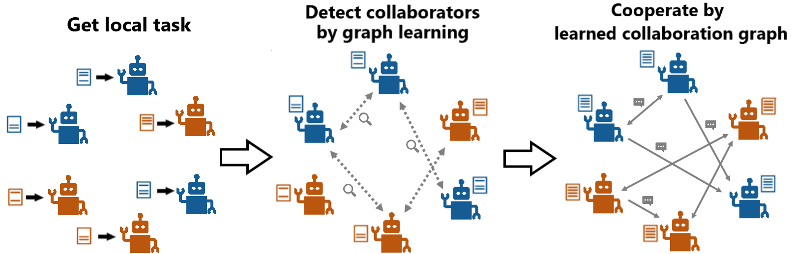
Fig. 1: Human-like distributed collaborative learning.

2 Related works

Collaborative learning. Two recent collaborative learning frameworks achieve tremendous successes, including federated learning and swarm learning. Federated learning enables multiple agents/organizations to collaboratively train a model [3, 5, 6, 4, 7]. Swarm learning promotes extensive studies about multi-agent collaboration mechanism [9, 10, 8, 11, 12, 13]. In this work, we propose a human-like collaborative learning framework, emphasizing collaboration relationship inference, which receives little attention in previous works.

Graph learning. Graph learning can be concluded as inferring graph-data topology by node feature[14, 15]. Typical graph learning (e.g. Laplacian inferring) can be solved by the optimization problem formulated by inter-nodal interaction[16, 17]. As traditional graph inference may fail when the objective cannot be well mathematically formulated, there are approaches applying graph deep learning models or algorithm unrolling [18, 19, 20, 21]. In this work, we leverage algorithm unrolling techniques to learn a graph structure, which combines both mathematical design and learning ability.

3 Methodology

3.1 Optimization problem

Consider a collaboration system with $N$ agents. Each agent is able to collect local data and collaborate with other agents for an overall optimization. Let $X_{i},Y_{i}$ be the observation and the supervision of the $i$th agent. The performance of a local model is evaluated by the loss ${\mathcal{L}}_{i}(X_{i},Y_{i};{\bm{\theta}}_{i})$ (${\mathcal{L}}_{i}({\bm{\theta}}_{i})$ for simplicity), where ${\bm{\theta}}_{i}\in\mathbb{R}^{M}$ is the model parameter of the $i$th agent. The pairwise collaboration between agents is formulated by a directed collaboration graph represented by the adjacency matrix $\mathbf{W}\in\mathbb{R}^{N\times N}$, whose $(i,j)$th element $w_{ij}$ reflects the collaboration weight from agent $i$ to $j$. Note that we do not consider self-loops so the diagonal elements of $\mathbf{W}$ are all zeros. Then the $i$th agent’s partners are indicated by a set of outgoing neighbours with nonzero edge weights; that is, $\mathcal{N}_{i}=\{{\rm Agent}~{}j|w_{ij}>0\}$. Inspired by social group-effect, agents are encouraged to find partners and imitate their parameters for less biased local model[1]. Therefore, the global optimization is formulated as:

$$\min_{\{{\bm{\theta}}_{i}\}_{i=1}^{N},\mathbf{W}}~{}\sum_{i=1}^{N}{\mathcal{L}}_{i}({\bm{\theta}}_{i})+\lambda_{1}\|\mathbf{W}\|_{F}^{2}+\lambda_{2}\!\sum_{i,j=1}^{N}w_{ij}\|{\bm{\theta}}_{i}\!-\!{\bm{\theta}}_{j}\|^{2}_{2}$$

$$~{}~{}~{}~{}~{}~{}{\rm subject~{}to~{}}~{}\ \|\mathbf{W}\|_{1}=N,w_{ii}=0,w_{ij}\geq 0,\forall i,j,$$ (1)

where $\lambda_{1},\lambda_{2}$ are predefined hyperparameters. The first term reflects all the local task-specific losses; the second term regularizes energy distribution of edge-weights; and the third term promotes graph smoothness; that is, agents with similar tasks tend to have similar model parameters and have higher demands to collaborate with each other.

However, in a distributed setting, there is no central server to handle the global optimization. To optimize (3.1) distributively, let $\mathbf{w}_{i}$ be the $i$th column of $\mathbf{W}$ and we consider the following local optimization for the $i$th agent:

$$\min_{{\bm{\theta}}_{i},\mathbf{w}_{i}}{\mathcal{L}}_{i}({\bm{\theta}}_{i})+\lambda_{1}\|\mathbf{w}_{i}\|_{2}^{2}+\lambda_{2}\sum_{j}w_{ij}\|{\bm{\theta}}_{i}-{\bm{\theta}}_{j}\|^{2}_{2}$$

$${\rm subject~{}to~{}}~{}\|\mathbf{w}_{i}\|_{1}=1,w_{ii}=0,w_{ij}\geq 0,\forall j.$$ (2)

Note that the feasible solution space of (3.1) is a subset of the feasible solution space of (3.1) because of the first constraint. Each agent has no perception of all the collaboration relationships and can only decide its outgoing edges. To solve problem (3.1), we consider an alternative solution, where each agent alternatively optimizes its ${\bm{\theta}}_{i}$ and $\mathbf{w}_{i}$. The overall procedure is shown in Algorithm 1, which contains two alternative steps:

Algorithm 1 Collaborative learning for Agent $i$

0:  

  Initialization: ${\bm{\theta}}_{i}^{(0)}\leftarrow{\arg\min_{\bm{\theta}}\ }{\mathcal{L}}_{i}({\bm{\theta}})$

  for $t\leftarrow 0\ \mathbf{to}\ T_{1}-1:$ do

     if $t\mod T_{2}=0$ then

        # broadcast and update $\mathbf{w}_{i}$

        Broadcast ${\bm{\theta}}_{i}^{(t)}$ to all agents

        Get $\mathbf{\Theta}^{(t)}=[{\bm{\theta}}_{1}^{(t)},...,{\bm{\theta}}_{N}^{(t)}]$ from other agents

        $\mathbf{w}_{i}\leftarrow$ graph_learning$(\mathbf{\Theta}^{(t)})$ by Algorithm 2 or 3

     else

        # only communicate with partners

        Send ${\bm{\theta}}_{i}^{(t)}$ to partners $\mathcal{N}_{i}=\{{\rm Agent}~{}j|w_{ij}>0\}$

        Get $\mathbf{\Theta}^{(t)}_{\mathcal{N}_{i}}=\{{\bm{\theta}}_{j}^{(t)}|w_{ij}>0\}$ from partners

     end if

     # update parameters

     ${\bm{\theta}}_{i}^{(t+1)}\leftarrow{\arg\min_{\bm{\theta}}\ }{\mathcal{L}}_{i}({\bm{\theta}})+\lambda_{2}\sum_{j\in\mathcal{N}_{i}}w_{ij}\|{\bm{\theta}}-{\bm{\theta}}_{j}^{(t)}\|^{2}$

  end for

  $\mathbf{{\bm{\theta}}}_{i},\mathbf{w}_{i}$

1) Graph learning. This step allows each agent to optimize who to collaborate with. Through broadcasting, the $i$th agent obtains all the other agents’ model parameters $\{{\bm{\theta}}_{j}^{(t)}|j\neq i\}$; and then optimizes its local relationships with others by solving the subproblem:

$$\min_{\mathbf{w}_{i}}~{}\lambda_{1}\|\mathbf{w}_{i}\|^{2}_{2}+\lambda_{2}\sum_{j}w_{ij}\|{\bm{\theta}}_{i}^{(t)}-{\bm{\theta}}_{j}^{(t)}\|^{2}_{2}$$ (3)

$${\rm subject~{}to~{}}~{}\|\mathbf{w}_{i}\|_{1}=1,w_{ii}=0,w_{ij}\geq 0,\forall j.$$

Since (3) is a convex problem, we optimize $\mathbf{w}_{i}$ via the standard dual-ascent method. Let $f(\mathbf{w}_{i})=\lambda_{1}\|\mathbf{w}_{i}\|^{2}_{2}+\lambda_{2}\sum_{j}w_{ij}\|{\bm{\theta}}_{i}^{(t)}-{\bm{\theta}}_{j}^{(t)}\|^{2}_{2}$. The dual-ascent updating step is,

$$\mathbf{w}_{i} \leftarrow\arg\min_{\mathbf{w}_{i}}~{}f(\mathbf{w}_{i})+z(\mathbf{1}^{\top}\mathbf{w}_{i}-1)+\mathcal{P}_{\mathbf{w}_{i}>0},$$

$$z~{}~{} \leftarrow z+p\cdot(\mathbf{1}^{\top}\mathbf{w}_{i}-1),$$

where $p$ is the stepsize and $\mathcal{P}_{\mathbf{w}_{i}>0}$ is a barrier function to ensure $w_{ij}\geq 0$. Until the convergence, we obtain the $i$th agent’s collaboration relationship for the next iterations to update ${\bm{\theta}}_{i}$. The detailed process is shown in Algorithm 2.

Algorithm 2 Dual-ascend for graph learning

0:  $\mathbf{\Theta}=[{\bm{\theta}}_{1},...,{\bm{\theta}}_{N}]\in\mathbb{R}^{M\times N},p=stepsize$

  $\mathbf{Initialization:}$ $\mathbf{w}_{i}\leftarrow(\mathbf{1}^{N-1})/(N-1),z\leftarrow 0$

  $\mathbf{Ensure:}$ $w_{ii}=0$

  $\mathbf{d}_{i}=[\|{\bm{\theta}}_{i}-{\bm{\theta}}_{1}\|_{2}^{2},...,\|{\bm{\theta}}_{i}-{\bm{\theta}}_{N}\|_{2}^{2}]$

  $\mathbf{Repeat:}$

     $\mathbf{w}_{i}\leftarrow{\rm ReLU}\left(-\frac{\lambda_{2}\mathbf{d}_{i}+z}{2\lambda_{1}}\right)$

     ${\rm diff}\leftarrow\mathbf{1}^{\top}\mathbf{w}_{i}-1$; $z\leftarrow z+p\cdot{\rm diff}$

  $\mathbf{Until:}$ Convergence

  $\mathbf{w}_{i}$

2) Parameter updating. This step allows each agent to update its local model by imitating its partners. Given the latest collaboration relationships $\mathbf{w}_{i}$ and the partners’ parameters, each agent obtains its new parameter ${\bm{\theta}}_{i}^{(t+1)}$ by optimizing:

$$\min_{{\bm{\theta}}_{i}}\ {\mathcal{L}}_{i}({\bm{\theta}}_{i})+\lambda_{2}\sum_{j}w_{ij}\|{\bm{\theta}}_{i}-{\bm{\theta}}_{j}^{(t)}\|^{2}_{2},$$ (4)

where ${\bm{\theta}}_{j}^{(t)}$ is the $j$th agent’s local model parameter in the $t$th iteration. To provide a general analytical solution, we could consider a second-order Taylor expansion to approximate the task-specific loss ${\mathcal{L}}_{i}$; that is,

$${\mathcal{L}}_{i}({\bm{\theta}}_{i})\approx\frac{1}{2}({\bm{\theta}}_{i}-\alpha_{i})^{\top}\mathbf{H}_{i}({\bm{\theta}}_{i}-\alpha_{i})+{\mathcal{L}}_{i}(\alpha_{i}),$$ (5)

where $\alpha_{i}={\arg\min_{\bm{\theta}}\ }{\mathcal{L}}_{i}({\bm{\theta}})$, which is solved by gradient descent in the initialization step, and $\mathbf{H}_{i}$ is the Hessian matrix of ${\mathcal{L}}_{i}$ at $\alpha_{i}$. By this approximation, the objective is in the form of a quadratic function determined by $\alpha_{i}$ and $\mathbf{H}_{i}$. Then, the optimization problem (4) becomes quadratic and we can obtain its analytical solution:

$${\bm{\theta}}^{(t+1)}_{i}\!=\!\big{(}\mathbf{H}_{i}\!+\!2\lambda_{2}\|\mathbf{w}_{i}\|_{1}\mathbf{I}\big{)}^{-1}\big{(}\mathbf{H}_{i}\alpha_{i}\!+\!2\lambda_{2}\sum\nolimits_{j}w_{ij}{\bm{\theta}}^{(t)}_{j}\big{)}.$$ (6)

To reduce communication cost, each agent executes parameter update by (6) without changing neighbour for $T_{2}$ rounds; and then, each agent will recalculate the collaboration relationship and update its partners. $T_{1}$ and $T_{2}$ are set empirically as long as ${\bm{\theta}}_{i}$ converges.

3.2 Unrolling of graph learning

The optimization problem (3.1) considers the quadratic term of graph Laplacian to promote graph smoothness, which is widely used in many graph-based applications. However, it has two major limitations. First, the $\ell_{2}$-distance might not be expressive enough to reflect the similarity between two models. Second, it is nontrivial to find appropriate hyperparameter $\lambda_{1}$ to attain effective collaboration graph. To address these issues, we propose a learnable collaboration term to promote more flexibility and expressiveness in learning collaboration relationships. We then solve the resulting graph learning optimization through algorithm unrolling.

Let $\mathbf{D}_{i}\in\mathbb{R}^{M\times N}$ be the $i$th agent’s parameter distance matrix whose $(m,j)$th element is $(\mathbf{D}_{i})_{mj}=({\bm{\theta}}_{im}-{\bm{\theta}}_{jm})^{2}$ with ${\bm{\theta}}_{im}$ the $m$th element of the $i$th agent’s model parameter ${\bm{\theta}}_{i}$. The original graph smoothness criteria can be reformulated as ${\bf 1}^{T}_{M}\mathbf{D}_{i}\mathbf{w}_{i}\ =\ \sum_{m=1}^{M}\sum_{j=1}^{N}({\bm{\theta}}_{im}-{\bm{\theta}}_{jm})^{2}w_{ij},$ where ${\bf 1}_{M}\in\mathbb{R}^{M}$ is an all-one vector. To make this term more flexible, we introduce trainable attention to reflect diverse importance levels of model parameters and reformulate the graph learning optimization as

$$\min_{\mathbf{w}_{i}}\ \frac{1}{2}\|\mathbf{Q}\mathbf{D}_{i}\mathbf{w}_{i}\|^{2}_{2}=\frac{1}{2}\sum_{m=1}^{M}\bigg{(}\sum_{j=1}^{N}q_{m}({\bm{\theta}}_{im}-{\bm{\theta}}_{jm})^{2}w_{ij}\bigg{)}^{2}$$

$$\quad{\rm subject~{}to~{}}\|\mathbf{w}_{i}\|_{1}=1,w_{ii}=0,w_{ij}\geq 0,\forall j,$$ (7)

where $\mathbf{Q}=\mathbf{diag}(q_{1},..q_{M})$ with $q_{k}>0$ reflecting the importance of the $m$th parameter. The new objective merges the original graph smoothness criteria and energy constraint. It is also quadratic to make the optimization easier. According to the proximal-descend procedure, when the stepsize is not so large, the optimizing iteration can be formulated as:

$$\mathbf{w}^{k+1}_{i}\leftarrow{\rm ReLU}\left({\rm Proj}_{\mathcal{D}}(\mathbf{I}-\mu\mathbf{D}_{i}^{\top}\mathbf{Q}^{2}\mathbf{D}_{i})\mathbf{w}_{i}^{k}\right),$$

where $\mu$ is the stepsize and projection ${\rm Proj}_{\mathcal{D}}$ is specified as:

$${\rm Proj}_{\mathcal{D}}(\mathbf{V})\equiv\mathbf{V}-\frac{(\mathbf{1}_{M}\mathbf{V}-1)\mathbf{1}_{M}}{M}.$$

To reduce parameter complexity, we use one diagonal matrix $\mathbf{P}=\mu\mathbf{Q}^{2}>\gamma$ to integrate $\mu$ and $\mathbf{Q}^{2}$. The $m$th element $p_{m}$ on the diagonal of $\mathbf{P}$ can be interpreted as the stepsize made by the smoothness of the $m$th parameter and $\gamma$ is a lower limit in training to avoid $p_{m}$ from degrading to 0. $\mathbf{P}$ can be supervised by loss ${\mathcal{L}}_{P}$ formulated by the average performance of all the agents with regard to actual local task. The unrolled forwarding of $K$ iterations is showed in Algorithm 3. For more adaptability, the output is not necessarily the actual solution to (7) , which means few iterations is needed and the output will be largely decided by $\mathbf{P}$.

Algorithm 3 Unrolled graph learning

0:  $\mathbf{\Theta}=[{\bm{\theta}}_{1},...,{\bm{\theta}}_{N}]^{\top}\in\mathbb{R}^{M\times N}$

  $\mathbf{Initialization:}$ $\mathbf{w}^{0}_{i}=(\mathbf{1}^{N-1})/(N-1)$

  $\mathbf{Ensure:}$ $w_{ii}=0$

  for $k\leftarrow 0\ \mathbf{to}\ K-1:$ do

     $\mathbf{w}_{i}^{k+1}={\rm ReLU[Proj}_{\mathcal{D}}(\mathbf{I}-\mathbf{D}_{i}^{\top}\mathbf{P}\mathbf{D}_{i})\mathbf{W}^{k}]$

  end for

  $\mathbf{w}_{i}=\mathbf{w}^{K}_{i}/\|\mathbf{w}^{K}_{i}\|_{1}$ # normalize

  $\mathbf{w}_{i}$

4 Experiments

Task/Method	No Colla.	Original GL	Unrolled GL	Fixed Colla.
Regression:
$L_{reg}$	16.1854	3.5332	2.9642	2.2294
GMSE	-	1.7683	0.8056	0
Classification:
ACC	0.6214	0.7268	0.7429	0.7481
GMSE	-	0.3115	0.1188	0

Table 1: Comparison on regression and classification tasks.

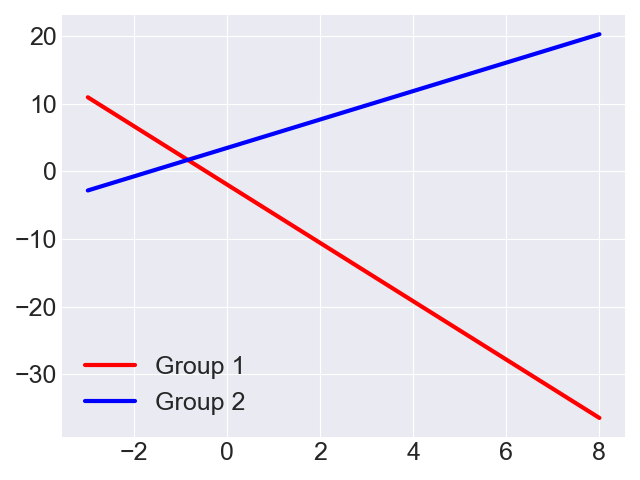
(a) Ground-truth lines.

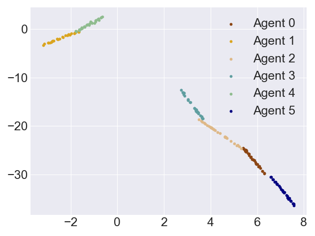
(b) Noisy samples.

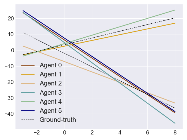
(c) Result without collaboration.

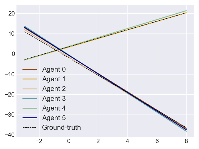
(d) Result by learned graph.

Fig. 2: A visualized example of data and result in regression.

To validate our model, we design two type of local tasks (regression and classification) and compare the performance of our unrolled network with different collaboration schemes.

4.1 Linear Regression

Dataset. We consider two different lines. Each agent only gets noisy samples from a segment of one line and aims to regress the corresponding line function, see Fig. 2. To achieve better regression, each agent can collaborate with other agents and get more information about the line. The challenges include: i) how to find partners that are collecting data from the same line; and ii) how to fuse information from other agents to obtain a better regression model.

Evaluation. We consider two evaluation metrics: one for regression and the other one for graph learning. Let the regression error be $L_{reg}=\frac{1}{N}\sum_{i=1}^{N}[(\widehat{k}_{i}-k_{i})^{2}+(\widehat{b}_{i}-b_{i})^{2}],$ where $\widehat{k}_{i},\widehat{b}_{i}$ are the line parameters estimated by the $i$th agent and $k_{i},b_{i}$ are the ground-truth line parameters of the $i$th agent. The graph structure is evaluated by ${\rm GMSE}=\frac{1}{N}\sum_{i=1}^{N}\|\mathbf{\widehat{w}}_{i}-\mathbf{w}_{i}\|_{F}^{2},$ $\mathbf{\widehat{w}_{i}}$ is the estimated edge-weights and $\mathbf{w}_{i}$ is the ground-truth edge-weights, where the edge-weights are uniformly distributed only among agents in the same task group fitting the same line.

Experimental setup. We compare four methods: i) local learning without collaboration; ii) collaboration by the predefined ground-truth graph; iii) collaboration by original optimization Algorithm 2 with well-tuned $\lambda_{1}$; and iv) collaboration by unrolled model Algorithm 3. We set the same $\lambda_{2}$ for all methods to ensure fairness. The unrolled model is pretrained on a training set and the hyperparameter $\mathbf{P}$ is supervised by the regression error $L_{reg}$. Then all models are tested on the same testing set including different partitions and data.

Results. Table 2 shows that i) collaboration brings significant benefits; ii) unrolling works better than pure optimization; iii) the unrolled graph is closer to the ground-truth graph. These results are expected because ${\bm{\theta}}_{i}=(k_{i},b_{i})^{\top}$ is non-Euclidean and the unrolled model can learn a more suitable evaluation than $\ell_{2}$-distance. Fig. 2 visualizes the regression results, which reflects the consistent patterns with Table 2.

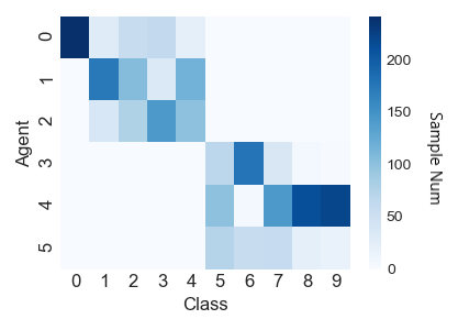
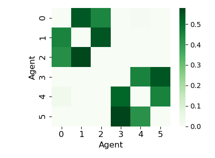
Fig. 3: Data distribution (left) and the learned collaboration weight matrix $\mathbf{W}$ (right) in one classification task.

4.2 Classification

Dataset. The dataset we adopt is a reduced MNIST. Original $28\times 28$ grid is processed by a pre-trained ResNet and reduced by PCA to a vector of $\mathbb{R}^{20}$. There are 10 types of samples. Agents are divided into two groups: group 1 classify type 1-5 and group 2 classify type 6-10. The samples are non-IID, see Fig. 3. The challenges also include how to find partners having the same data category and how to fuse information for less biased perception.

Evaluation. Similarly, there are two evaluation metrics: the classification performance is evaluated by agents’ average ACC and graph learning is evaluated by $\rm GMSE$.

Experimental setup. The baselines and testing process are the same as 4.1. Differently, the local model at each agent is a linear classifier for 5 classes and ${\mathcal{L}}_{i}({\bm{\theta}}_{i};X_{i},Y_{i})$ is defined as the cross-entropy loss function. Because there is no ground-truth local parameter, in pretraining the unrolled hyperparameter $\mathbf{P}$ is supervised by ${\mathcal{L}}_{P}=\sum_{i=1}^{N}{\mathcal{L}}_{i}({\bm{\theta}}_{i};X_{i},Y_{i})$.

Results. The results are also shown in Table 2. Note that the unrolled model gains a more obvious enhancement than 4.1 as local parameter has higher dimension. A visualized example of the learned matrix $\mathbf{W}$ is shown in Fig. 3.

5 Conclusion and future work

We proposed a distributed multi-agent learning model inspired by human collaboration and an unrolled model for collaboration graph learning. By experiments in different tasks, we verify that: i) our human-like collaboration scheme is feasible; ii) our unrolled graph learning can improve performance in various tasks. Currently, the local tasks in our experiments are rudimentary trials. In future works, we will apply our framework to more complicated nonlinear local models for more versatility.

Appendix

Task	Regression		Classification
/ Method	$L_{reg}~{}(\downarrow)$	GMSE $(\downarrow)$	ACC $(\uparrow)$	GMSE $(\downarrow)$
No Colla. (Lower bound)	16.1854	-	0.6214	-
Graph Lasso[Mazumder2011TheGL]	7.6042	4.6187	0.6787	1.1829
L2G-ADMM[2110.0980]	3.9842	1.6916	0.7166	2.0248
Unrolled GL (Ours)	2.9642	0.8056	0.7429	0.1188
Fixed Colla. (Upper bound)	2.2294	0	0.7481	0

Table 2: Comparisons with two additional baselines

A. Comparison with other baselines

To make a more comprehensive comparison, we also introduce two additional baselines: Graphical Lasso and L2G-ADMM. Graphical Lasso is a classical graph learning algorithm for undirected Gaussian graphical model Mazumder2011TheGL. L2G-ADMM is a model-based graph Laplacian learning method solved by ADMM 2110.0980. Note that both of the two baselines are centralized methods.

The results are shown in Table 2. We can see that the proposed unrolled method significantly outperforms two baselines. That is because our distributed model has regularization for each column for $\mathbf{W}$, which can encourage each agent to refer to others’ parameters. By contrast, L2G-ADMM does not have regularization specifically designed for collaboration. Graphical Lasso is not reliable when the number of local parameters $M$ is small ( local model parameters are $M$ samples of $N$-dimensional Gaussian distribution).

B. Parameter settings in our experiments

The settings of critical parameters in the experiment are listed below:

• To ensure the same collaboration weight, we set $\lambda_{2}=0.1$ for all the collaborative methods.

• In regression tasks $\lambda_{1}=3$ and in classification tasks $\lambda_{1}=0.05$ (tuned by grid search on the training set).

• In both tasks, the unrolling steps $K=10$.

• To compare the performance under limited collaboration times, in both tasks $T_{1}/T_{2}=2$, which means the agents can change collaborators for 2 times. We set $T_{2}$ large enough to ensure the convergence (10 for regression and 200 for classification).

In regression tasks, each agent gets 100 sample points. In classification tasks, each agent gets about 250 samples. The local samples for each agent will not change in one test.

References

IEEEbib ref2

References

- [1] Abdullah Almaatouq, Alejandro Noriega-Campero, Abdulrahman Alotaibi, PM Krafft, Mehdi Moussaid, and Alex Pentland, “Adaptive social networks promote the wisdom of crowds,” Proceedings of the National Academy of Sciences, vol. 117, no. 21, pp. 11379–11386, 2020.
- [2] Liviu Panait and Sean Luke, “Cooperative multi-agent learning: The state of the art,” Autonomous agents and multi-agent systems, vol. 11, no. 3, pp. 387–434, 2005.
- [3] Alysa Ziying Tan, Han Yu, Lizhen Cui, and Qiang Yang, “Towards personalized federated learning,” IEEE Transactions on Neural Networks and Learning Systems, 2022.
- [4] Stefanie Warnat-Herresthal, Hartmut Schultze, Krishnaprasad Lingadahalli Shastry, Sathyanarayanan Manamohan, Saikat Mukherjee, Vishesh Garg, Ravi Sarveswara, Kristian Händler, Peter Pickkers, N Ahmad Aziz, et al., “Swarm learning for decentralized and confidential clinical machine learning,” Nature, vol. 594, no. 7862, pp. 265–270, 2021.
- [5] Tian Li, Anit Kumar Sahu, Ameet Talwalkar, and Virginia Smith, “Federated learning: Challenges, methods, and future directions,” IEEE Signal Processing Magazine, vol. 37, no. 3, pp. 50–60, 2020.
- [6] Nicola Rieke, Jonny Hancox, Wenqi Li, Fausto Milletari, Holger R Roth, Shadi Albarqouni, Spyridon Bakas, Mathieu N Galtier, Bennett A Landman, Klaus Maier-Hein, et al., “The future of digital health with federated learning,” NPJ digital medicine, vol. 3, no. 1, pp. 1–7, 2020.
- [7] Anusha Lalitha, Shubhanshu Shekhar, Tara Javidi, and Farinaz Koushanfar, “Fully decentralized federated learning,” in Third workshop on Bayesian Deep Learning (NeurIPS), 2018.
- [8] Soma Minami, Tsubasa Hirakawa, Takayoshi Yamashita, and Hironobu Fujiyoshi, “Knowledge transfer graph for deep collaborative learning,” in Proceedings of the Asian Conference on Computer Vision, 2020.
- [9] Zhanhong Jiang, Aditya Balu, Chinmay Hegde, and Soumik Sarkar, “Collaborative deep learning in fixed topology networks,” Advances in Neural Information Processing Systems, vol. 30, 2017.
- [10] Mohammad Rostami, Soheil Kolouri, Kyungnam Kim, and Eric Eaton, “Multi-agent distributed lifelong learning for collective knowledge acquisition,” in Proceedings of the 17th International Conference on Autonomous Agents and MultiAgent Systems, Richland, SC, 2018, AAMAS ’18, p. 712–720, International Foundation for Autonomous Agents and Multiagent Systems.
- [11] Yiming Li, Shunli Ren, Pengxiang Wu, Siheng Chen, Chen Feng, and Wenjun Zhang, “Learning distilled collaboration graph for multi-agent perception,” Advances in Neural Information Processing Systems, vol. 34, pp. 29541–29552, 2021.
- [12] Zixing Lei, Shunli Ren, Yue Hu, Wenjun Zhang, and Siheng Chen, “Latency-aware collaborative perception,” arXiv preprint arXiv:2207.08560, 2022.
- [13] Yue Hu, Shaoheng Fang, Zixing Lei, Yiqi Zhong, and Siheng Chen, “Where2comm: Communication-efficient collaborative perception via spatial confidence maps,” arXiv preprint arXiv:2209.12836, 2022.
- [14] Gonzalo Mateos, Santiago Segarra, Antonio G. Marques, and Alejandro Ribeiro, “Connecting the dots: Identifying network structure via graph signal processing,” IEEE Signal Processing Magazine, vol. 36, no. 3, pp. 16–43, 2019.
- [15] Xiaowen Dong, Dorina Thanou, Michael Rabbat, and Pascal Frossard, “Learning graphs from data: A signal representation perspective,” IEEE Signal Processing Magazine, vol. 36, no. 3, pp. 44–63, 2019.
- [16] Xiaowen Dong, Dorina Thanou, Pascal Frossard, and Pierre Vandergheynst, “Learning laplacian matrix in smooth graph signal representations,” IEEE Transactions on Signal Processing, vol. 64, no. 23, pp. 6160–6173, 2016.
- [17] Yan Leng, Xiaowen Dong, Junfeng Wu, and Alex Pentland, “Learning quadratic games on networks,” in Proceedings of the 37th International Conference on Machine Learning. 2020, ICML’20, JMLR.org.
- [18] Emanuele Rossi, Federico Monti, Yan Leng, Michael Bronstein, and Xiaowen Dong, “Learning to infer structures of network games,” in International Conference on Machine Learning. PMLR, 2022, pp. 18809–18827.
- [19] Xingyue Pu, Tianyue Cao, Xiaoyun Zhang, Xiaowen Dong, and Siheng Chen, “Learning to learn graph topologies,” Advances in Neural Information Processing Systems, vol. 34, pp. 4249–4262, 2021.
- [20] Vishal Monga, Yuelong Li, and Yonina C Eldar, “Algorithm unrolling: Interpretable, efficient deep learning for signal and image processing,” IEEE Signal Processing Magazine, vol. 38, no. 2, pp. 18–44, 2021.
- [21] Nir Shlezinger, Yonina C Eldar, and Stephen P Boyd, “Model-based deep learning: On the intersection of deep learning and optimization,” arXiv preprint arXiv:2205.02640, 2022.

References

IEEEbib \bibliographysecref2