Dynamics of an HIV/AIDS transmission model with protection awareness and fluctuations

Abstract

We establish a stochastic HIV/AIDS model for the individuals with protection awareness and reveal how the protection awareness plays its important role in the control of AIDS. We firstly show that there exists a global positive solution for the stochastic model. By constructing Lyapunov functions, the ergodic stationary distribution when $R_{0}^{s}>1$ and the extinction when $R_{0}^{e}<1$ for the stochastic model are obtained. A number of numerical simulations by using positive preserving truncated Euler-Maruyama method (PPTEM) are performed to illustrate the theoretical results. Our new results show that the detailed publicity has great impact on the control of AIDS compared with the extensive publicity, while the continuous antiretroviral therapy (ART) is helpful in the control of HIV/AIDS.

1 Introduction

Infectious diseases caused one-quarter of the global deaths ref1 . Various factors such as media campaigns, population migration and temperature changes influenced the spreading of infectious diseases. Since June 6 of 1981, the first global case of HIV (Human Immunodeficiency Virus) infection was announced, human beings have been fighting against HIV for over four decades. As of the year 2022, about 37.7 million individuals have been infected with HIV ref2 . As we have known today, the transmission of HIV took place through blood, semen, cervical (or, vaginal secretions) and breast milk as well. Especially, an infected individual was unaware of the protection and was lack of active treatment, HIV often broke down the immune system of the infected individual and eventually turned into the acquired immune deficiency syndrome (AIDS). Although there was no drug or vaccine for HIV, the antiretroviral therapy (ART) could prolong the life expectancy of an infected individual and make it approach that of the uninfected individuals. Meanwhile, the infected individuals with ART treatment do not retransmit HIV to their sexual partners ref2 . From 2000 to 2018, the number of new HIV infected individuals fell by 37%, HIV-related deaths fell by 45%, and ART treatment saved 13.6 million individuals. At the end of 2018, about 23.3 million individuals had received ART treatment ref2 . Thus, UNAIDS puts forward the 90%-90%-90% plan(90% of AIDS infected people know they are infected, 90% of confirmed AIDS patients to be treated, and 90% of HIV in treated patients’ body is suppressed), and set the great goal of eliminating the AIDS epidemic by 2030 in UN General Assembly Resolution 70/266.

Mathematical modelling of HIV/AIDS and its kinetic behavior analysis can well predict the development trend of HIV/AIDS. Many scholars have already studied the HIV/AIDS model and its kinetic behavior. For example, Silva and Torres ref3 obtained the results on the global stability of the HIV/AIDS model by considering bilinear incidence rates. Ghosh et al. ref4 studied the effect of medias and self-imposed psychological fears on disease dynamics by separating the susceptible into the unaware and the aware individuals. Later, Zhao et al. ref6 modified the model established by Fatmawati et al. ref5 , and considered piecewise fractional differential equations and investigated the effect of protection awareness on HIV transmission. However, the transmissions of infectious disease were inevitably affected by the environmental noises in the real circumstances. In other words, the numbers of the individuals in each compartment were usually fluctuated due to the emergence of infectious disease and control as well by local governments. Therefore, the epidemic models with fluctuations in practice were necessary to investigate their long-term dynamics. For instance, Mao et al. ref7 found that the small fluctuations to the deterministic models effectively suppress the rapid increment of the population. Other recent epidemic models in ref8 ; ref9 ; ref10 ; ref11 ; ref12 ; ref13 ; ref13.2 ; ref13.3 also governed the fluctuations to describe the diversities of their models. More precisely, ref13.2 ; ref13.3 found that small fluctuations produced the long-term persistence, and large fluctuations led to the extinction of infectious diseases in stochastic HIV/AIDS models. Liu ref13.4 discovered that the higher order fluctuations made HIV/AIDS eradicative under sufficient conditions. Meanwhile, Wang ref13.5 also figured out the extinction and persistence in the mean depended on the fluctuations of main parameters.

We formulate a stochastic HIV/AIDS model with protection awareness by considering the environmental noises into the model of Fatmawati et al. ref5 . We next provide the expression of the basic reproduction number for the deterministic model. In Section 3, we prove theoretically that there exists a unique positive solution to the stochastic model, and the existence of a unique ergodic stationary distribution is investigated. Further, we give a new threshold $R_{0}^{e}$ for the extinction of HIV/AIDS, and the corresponding numerical simulations are demonstrated to verify the theoretical results. Then we conclude that the detailed publicity has great impact on the control of AIDS compared with the extensive publicity. Moreover, the continuous antiretroviral therapy (ART) is helpful to control the number of the individuals with HIV/AIDS. Meanwhile, we figure out the main improvements compared with other contributions, and give some suggestions to control the long-term dynamics of HIV/AIDS.

2 Establishment of the mathematical model

The number that an infected contacts with the susceptible per unit of time is called the contact number, which is usually related to the total population $N$ and denoted as $U(N)$. Let the probability of infection per exposed individual be $\beta_{0}$, and $\beta_{0}U(N)$ is called the effective exposure number, which represents the infectivity of an infected individual per unit of time. The total population is usually separated by the susceptible individuals, the immune individuals, and the exposed individuals. So, the proportion of the susceptible individuals in the whole population is ${\frac{S(t)}{N(t)}}$, which is not being infected by the infected individuals. Then, the number of the susceptible being infected effectively at time $t$ is

$$\beta_{0}U(N)\frac{S(t)}{N(t)}I(t)$$

which is called the incidence rate. We assume in this paper that the contact rate between the susceptible and the infected is proportional to the total population, i.e., $U(N)=kN(t)$. Let $\beta=\beta_{0}k$, then the incidence rate is rewritten as $\beta S(t)I(t)$, which is called the bilinear incidence rate. Many researchers have applied the bilinear incidence rates into their HIV/AIDS models ref14 ; ref15 ; ref16 ; ref17 for further discussions.

Fatmawati et al. ref5 developed a model of HIV/AIDS with the protection awareness. Precisely, they divided the population into five different groups, that is, the susceptible without protection awareness $(S_{u})$, the susceptible with protection awareness $(S_{a})$, the infected without ART treatment $(I)$, the infected with ART treatment $(C)$ and the infected who eventually developed into AIDS $(A)$. And, the total people size $N$ is expressed as

$$N=S_{a}+S_{u}+I+C+A.$$

We simplified the model of Fatmawati et al. ref5 by considering bilinear incidence:

$$\begin{array}[]{lll}\dot{S_{u}}(t)&=&\Lambda-\beta S_{u}I-(\alpha+\mu)S_{u},\\ \dot{S_{a}}(t)&=&\alpha S_{u}-(1-\varepsilon)\beta S_{a}I-\mu S_{a},\\ \dot{I}(t)&=&\beta I\left(S_{u}+(1-\varepsilon)S_{a}\right)+\eta C+vA-(\rho+\gamma+\mu)I,\\ \dot{C}(t)&=&\rho I-(\eta+\mu)C,\\ \dot{A}(t)&=&\gamma I-(v+\delta+\mu)A,\end{array}$$

where $\Lambda$ is the recruitment rate, $\mu$ is the natural death rate, and $\delta$ is the mortality rate of AIDS. $\alpha$ is the migration rate from $S_{u}$ to $S_{a}$, $\beta$ is the HIV transmission rate, and $\varepsilon$ is the infection rate of $S_{a}$. The parameters $\eta$, $\nu$, $\gamma$, and $\rho$ represent the transmission rates from $C$ to $I$, $A$ to $I$, $I$ to $A$ and $I$ to $C$. The mutual migrating mechanisms of each group in the model could be demonstrated clearly in Figure 2.1. We suppose that all parameters of model (2.1) are positive initiated with

$$\begin{array}[]{ll}&S_{u}(0)=S_{u0}\geq 0,S_{a}(0)=S_{a0}\geq 0,I(0)=I_{0}\geq 0,\\ &C(0)=C_{0}\geq 0,A(0)=A_{0}\geq 0.\end{array}$$

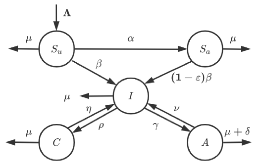
Figure 2.1 Propagation mechanism

Now, we add five equations of model (2.1) and then we get

$$\dot{N}(t)=\Lambda-\mu N-\delta A\leq\Lambda-\mu N.$$

By comparing theorems, the positive invariant set of model (2.1) is derived

$$\Omega=\left\{\left(S_{u},S_{a},I,C,A\right)\in\mathbb{R}_{+}^{5}:0\leq N\leq\frac{\Lambda}{\mu}\right\}.$$

We only consider the biological properties of model (2.1) in the set $\Omega$. The basic regeneration number of model (2.1) can be obtained from the next generation matrix approach ref17.1 ; ref17.2 as follows:

$$\begin{array}[]{ll}R_{0}=\displaystyle\frac{\beta\left[\mu+\left(1-\varepsilon\right)\alpha\right]k_{1}k_{2}\Lambda}{\mu(\mu+\alpha)\left[\mu\left(k_{2}\left(k_{1}+\gamma\right)+\rho k_{1}+\gamma\delta\right)+\eta\gamma\delta\right]},\end{array}$$

with $k_{1}=\mu+\delta+\nu$, $k_{2}=\mu+\eta$.

Similarly to the proof of Theorem 2 in Fatmawati et al. ref5 , when $R_{0}<1$, we obtain that model (2.1) has a unique boundary equilibrium point

$$P_{0}=\left(\frac{\Lambda}{\mu+\alpha},\frac{\alpha\Lambda}{\mu\left(\mu+\alpha\right)},0,0,0\right),$$

which is locally asymptotically stable in the set $\Omega$. We also provide the expression of an endemic equilibrium point of model (2.1) when $R_{0}>1$, that is

$$P^{\ast}=(S_{u}^{\ast},S_{a}^{\ast},I^{\ast},C^{\ast},A^{\ast}),$$

where

$$S_{u}^{\ast}=\frac{\Lambda}{\beta I^{\ast}+\alpha+\mu},S_{a}^{\ast}=\frac{\alpha\Lambda}{(\left(1-\varepsilon\right)\beta I^{\ast}+\mu)(\beta I^{\ast}+\alpha+\mu)},$$

$$C^{\ast}=\frac{\rho I^{\ast}}{k_{2}},A^{\ast}=\frac{\gamma I^{\ast}}{k_{1}}.$$

Substituting $S_{u}^{\ast}$, $S_{a}^{\ast}$, $C^{\ast}$, $A^{\ast}$ into the third equation of (2.1) and making the left side be zero, then we can get

$$f\left(I^{\ast}\right)= \beta I^{\ast}\left(\frac{\Lambda}{\beta I^{\ast}+\alpha+\mu}+\frac{(1-\varepsilon)\alpha\Lambda}{\left(\left(1-\varepsilon\right)\beta I^{\ast}+\mu\right)\left(\beta I^{\ast}+\alpha+\mu\right)}\right)+\eta\frac{\rho I^{\ast}}{k_{2}}$$

$$+\upsilon\frac{\gamma I^{\ast}}{k_{1}}-\left(\rho+\gamma+\mu\right)I^{\ast}$$

$$= I^{\ast}\left(\beta\Lambda k_{1}k_{2}\left(\left(1-\varepsilon\right)\beta I^{\ast}+\mu\right)+\beta\Lambda k_{1}k_{2}\left(1-\varepsilon\right)\alpha\right.$$

$$\left.+\left(k_{1}\eta\rho+k_{2}\upsilon\gamma-k_{1}k_{2}\left(\rho+\gamma+\mu\right)\right)\left(\beta I^{\ast}+\alpha+\mu\right)\left(\left(1-\varepsilon\right)\beta I^{\ast}+\mu\right)\right)$$

$$\left(k_{1}k_{2}\left(\beta I^{\ast}+\alpha+\mu\right)\left(\left(1-\varepsilon\right)\beta I^{\ast}+\mu\right)\right)^{-1}$$

$$= I^{\ast}(A^{\ast}{I^{\ast}}^{2}+B^{\ast}I^{\ast}+C^{\ast})\left(k_{1}k_{2}\left(\beta I^{\ast}+\alpha+\mu\right)\left(\left(1-\varepsilon\right)\beta I^{\ast}+\mu\right)\right)^{-1},$$

where

$$P_{1}= \left(1-\varepsilon\right)\beta^{2}\left(k_{1}\eta\rho+k_{2}\upsilon\gamma-k_{1}k_{2}\left(\rho+\gamma+\mu\right)\right)$$

$$= -\left(1-\varepsilon\right)\beta^{2}\left(\mu\upsilon\rho+\mu\delta\rho+\mu^{2}\rho+\eta\delta\rho+\eta\mu\rho+\mu\delta\gamma+\mu^{2}\gamma\right.$$

$$\left.+\mu\left(\nu+\delta+\mu\right)\left(\eta+\mu\right)\right)<0,$$

$$P_{2}= \beta\left(\left(1-\varepsilon\right)\alpha+\left(2-\varepsilon\right)\mu\right)\left(k_{1}\eta\rho+k_{2}\upsilon\gamma-k_{1}k_{2}\left(\rho+\gamma+\mu\right)\right)$$

$$+k_{1}k_{2}\Lambda\beta^{2}\left(1-\varepsilon\right),$$

$$P_{3}= k_{1}k_{2}\Lambda\beta\left(\mu+\left(1+\varepsilon\right)\alpha\right)+\mu\left(\mu+\alpha\right)\left(\ k_{1}\eta\rho+k_{2}\upsilon\gamma-k_{1}k_{2}\left(\rho+\gamma+\mu\right)\right)$$

$$= \mu\left(\mu+\alpha\right)\left(\mu\left[k_{2}\left(k_{1}+\gamma\right)+\rho k_{1}+\gamma\delta\right]+\eta\gamma\delta\right)\left(R_{0}-1\right).$$

Obviously $f(0)=0$. When $R_{0}>1$, we have $P_{1}<0$ and $P_{3}>0$. According to the Descartes sign rule, $f(I^{\ast})$ has a unique positive real root regardless of the sign of $P_{2}$. Therefore, the endemic equilibrium point $P^{\ast}$ exists.

Motivated by the models described by stochastic differential equations in ref18 ; ref19 ; ref20 ; ref21 ; ref22 , we introduce the environmental fluctuations into model (2.1) similar to that of Evansref22.1 and Tanref22.2 . We set that environmental fluctuations are multiplicative white noise types which are proportional to $S_{u},S_{a},I,C,A$. When $\Delta t\rightarrow 0$, we consider a Markov process

$$X(t)=\left(S_{u}(t),S_{a}(t),I(t),C(t),A(t)\right)^{T}$$

with the following descriptions:

$$\mathbb{E}[S_{u}(t+\Delta t)-S_{u}(t)|X_{t}=x]\thickapprox\left[\Lambda-\beta S_{u}(t)I(t)-(\alpha+\mu)S_{u}(t)\right]\Delta t,$$

$$\mathbb{E}[S_{a}(t+\Delta t)-S_{a}(t)|X_{t}=x]\thickapprox\left[\alpha S_{u}(t)-(1-\varepsilon)\beta S_{a}(t)I(t)-\mu S_{a}(t)\right]\Delta t,$$

$$\mathbb{E}[I(t+\Delta t)-I(t)|X_{t}=x]\thickapprox\left[\beta I(t)\left(S_{u}(t)+(1-\varepsilon)S_{a}(t)\right)+\eta C(t)+vA(t)\right.$$

$$\left.\hskip 125.50021pt-(\rho+\gamma+\mu)I(t)\right]\Delta t,$$

$$\mathbb{E}[C(t+\Delta t)-C(t)|X_{t}=x]\thickapprox[\rho I(t)-(\eta+\mu)C(t)]\Delta t,$$

$$\mathbb{E}[A(t+\Delta t)-A(t)|X_{t}=x]\thickapprox[\gamma I(t)-(v+\delta+\mu)A(t)]\Delta t,$$

and

$$\mbox{Var}[S_{u}(t+\Delta t)-S_{u}(t)|X_{t}=x]\thickapprox\sigma_{1}^{2}S_{u}^{2}(t)\Delta t,$$

$$\mbox{Var}[S_{a}(t+\Delta t)-S_{a}(t)|X_{t}=x]\thickapprox\sigma_{2}^{2}S_{a}^{2}(t)\Delta t,$$

$$\mbox{Var}[I(t+\Delta t)-I(t)|X_{t}=x]\thickapprox\sigma_{3}^{2}I^{2}(t)\Delta t,$$

$$\mbox{Var}[C(t+\Delta t)-C(t)|X_{t}=x]\thickapprox\sigma_{4}^{2}C^{2}(t)\Delta t,$$

$$\mbox{Var}[A(t+\Delta t)-A(t)|X_{t}=x]\thickapprox\sigma_{5}^{2}A^{2}(t)\Delta t.$$

We therefore derive a stochastic epidemic model as follows:

$$\begin{array}[]{lll}\mbox{d}S_{u}(t)&=&\left[\Lambda-\beta S_{u}(t)I(t)-(\alpha+\mu)S_{u}(t)\right]\mbox{d}t+\sigma_{1}S_{u}(t)\mbox{d}B_{1}(t),\\ \mbox{d}S_{a}(t)&=&\left[\alpha S_{u}(t)-(1-\varepsilon)\beta S_{a}(t)I(t)-\mu S_{a}(t)\right]\mbox{d}t+\sigma_{2}S_{a}(t)\mbox{d}B_{2}(t),\\ \mbox{d}I(t)&=&\left[\beta I(t)\left(S_{u}(t)+(1-\varepsilon)S_{a}(t)\right)+\eta C(t)+vA(t)\right.\\ &&\left.-(\rho+\gamma+\mu)I(t)\right]\mbox{d}t+\sigma_{3}I(t)\mbox{d}B_{3}(t),\\ \mbox{d}C(t)&=&[\rho I(t)-(\eta+\mu)C(t)]\mbox{d}t+\sigma_{4}C(t)\mbox{d}B_{4}(t),\\ \mbox{d}A(t)&=&[\gamma I(t)-(v+\delta+\mu)A(t)]\mbox{d}t+\sigma_{5}A(t)\mbox{d}B_{5}(t).\end{array}$$

Let $i=1,2,3,4,5$, then $B_{i}(t)$ are independent standard Brownian motions with the initial values $B_{i}\left(0\right)=0$ and $\sigma_{i}^{2}>0$ are the intensities of white noises, and the initial values $X(0)=(S_{u}(0),S_{a}(0),I(0),C(0),A(0))^{T}$ as well.

3 Existence and uniqueness of positive solution

Let $X(t)$ be a homogeneous markov process in $\mathbb{R}^{d}$, which satisfies the stochastic differential equation

$$\mbox{d}X(t)=b(x)\mbox{d}t+\sum_{r=1}^{k}{g_{r}\left(x\right)\mbox{d}B_{r}(t)},\quad k\leq d.$$

The diffusion matrix is defined as

$$A(X)=(a_{ij}(X))_{d\times d},\quad a_{ij}(X)=\sum_{r=1}^{k}{g_{r}^{i}(X)g_{r}^{j}(X).}$$

Lemma 3.1 ref23 Assume that there exists a bounded open region $G\subset\mathbb{R}^{d}$ with regular boundaries $\Gamma$, and it has the following properties:

(i) The minimum eigenvalue of the diffusion matrix $A(X)$ is non-zero in its domain $G$ and one of its neighborhoods.

(ii) The average time $\tau$ for the path from $z$ to set $G$ is finite when $z\in\mathbb{R}^{d}\backslash G$, and $\sup_{z\in K}E^{z}\tau<\infty$ holds for each compact subset $K\in\mathbb{R}^{d}$.

Then, the Markov process $X(t)$ has a unique ergodic stationary distribution $\pi(\cdot)$. Let $f(X)$ be an integrable function of $\pi$, for all $X\in\mathbb{R}^{d}$, the following formula holds:

$$\mathbb{P}\left\{\lim_{t\rightarrow\infty}{\frac{1}{t}\int_{0}^{t}f\left(X(s)\right)\mbox{d}s=\int_{\mathbb{R}^{d}}{f(X)\pi(\mbox{d}X)}}\right\}=1.$$

Remark 3.1 The proof of Lemma 3.1 can be found on pages 106-109 of Khasminskii ref23 . If there exists a positive $M$ such that

$$\sum_{i,j=1}^{d}{a_{ij}\left(X\right)\xi_{i}\xi_{j}}\geq M\left|\xi\right|^{2},\xi\in\mathbb{R}^{d},$$

then property (i) holds.

Now, we will give two useful results, Lemma 3.2 and Lemma 3.3, by using of Theorem 2.1 and Theorem 3.1 in ref27 . In fact, we write down the conclusions without consider the details of the proofs.

Lemma 3.2 Let $X(t)$ be a solution of $(2.3)$ initiated with $X_{0}\in\mathbb{R}_{+}^{5}$, then

$$\lim_{t\rightarrow\infty}{\frac{1}{t}\left(S_{u}(t)+S_{a}(t)+I(t)+C(t)+A(t)\right)}=0,$$

and

$$\lim_{t\rightarrow\infty}{\frac{S_{u}(t)}{t}}=0,\lim_{t\rightarrow\infty}{\frac{S_{a}(t)}{t}}=0,\lim_{t\rightarrow\infty}{\frac{I(t)}{t}}=0,$$

$$\lim_{t\rightarrow\infty}{\frac{C(t)}{t}}=0,\lim_{t\rightarrow\infty}{\frac{A(t)}{t}}=0\hskip 10.00002pt\text{a.s.}$$

Lemma 3.3 Suppose that $\mu>(\sigma_{1}^{2}\vee\sigma_{2}^{2}\vee\sigma_{3}^{2}\vee\sigma_{4}^{2}\vee\sigma_{5}^{2})/2$, let $X(t)$ be a solution of $(2.3)$ initiated with $X_{0}\in\mathbb{R}_{+}^{5}$. Then

$$\lim_{t\rightarrow\infty}{\frac{1}{t}\int_{0}^{t}{S_{u}(s)}\mbox{d}B_{1}(s)}=0,\lim_{t\rightarrow\infty}{\frac{1}{t}\int_{0}^{t}{S_{a}(s)}\mbox{d}B_{2}(s)}=0,$$

$$\lim_{t\rightarrow\infty}{\frac{1}{t}\int_{0}^{t}{I(s)}\mbox{d}B_{3}(s)}=0,\lim_{t\rightarrow\infty}{\frac{1}{t}\int_{0}^{t}{C(s)}\mbox{d}B_{4}(s)}=0,$$

$$\lim_{t\rightarrow\infty}{\frac{1}{t}\int_{0}^{t}{A(s)}\mbox{d}B_{5}(s)}=0\hskip 10.00002pt\text{a.s.}$$

Before we start to study the dynamical behaviors of the stochastic epidemic model (2.3), the existence of a global positive solution is of importance. Next, we show that there exists a unique global positive solution to (2.3) for any given initial value.

Theorem 3.1 Model $(2.3)$ has a unique global positive solution $X(t)\in\mathbb{R}_{+}^{5}$ initiated with $X_{0}\in\mathbb{R}_{+}^{5}$ for any $t\geq 0$.

Proof It is obvious to check that the local Lipschitz condition is satisfied for model (2.3) initiated with $X_{0}\in\mathbb{R}_{+}^{5}$, so there exists a unique local solution $X(t)$ for $t\in[0,\tau_{e})$. To prove that $X(t)$ is global, our work is to verify $\tau_{e}=\infty$. Indeed, let $n_{0}>1$ be large enough satisfying each component of $X(t)$ lies in $[{\frac{1}{n_{0}}},n_{0}]$. Define the stopping time

$$\begin{array}[]{lll}{\tau_{n}}=&\inf\left\{t\in[0,\tau_{e}):\min{\left\{S_{u}(t),S_{a}(t),I(t),C(t),A(t)\right\}}\leq\displaystyle\frac{1}{n}\right.\\ &\quad\left.\text{or}\hskip 2.84526pt\max{\left\{S_{u}(t),S_{a}(t),I(t),C(t),A(t)\right\}}\geq n\right\}\end{array}$$

for any integer $n>n_{0}$. Let $\inf\varnothing=\infty$. As $n\rightarrow\infty$, it is obvious that $\left\{\tau_{n}\right\}_{n\geq n_{0}}$ is monotonically increasing. We set $\tau_{\infty}=\lim_{n\to\infty}{\tau_{n}}$, then we get $\tau_{\infty}\leq\tau_{e}$ by the definition of stopping time. We claim that $\tau_{\infty}=\infty$. What we claim is checked, which ends the proof. By contradiction, there exists a pair of positvie constants $T>0$ and $\varepsilon\in(0,1)$ such that the probability that $\tau_{\infty}\leq T$ is larger than $\varepsilon$. We rewrite as $\mathbb{P}\left\{\tau_{n}\leq T\right\}\geq\varepsilon$ for $n\geq n_{0}$. Define a $C^{2}$-function $U:\mathbb{R}_{+}^{5}\rightarrow\mathbb{R}_{+}$ by

$$U\left(x\right)= \left(S_{u}-\theta-\theta\ln\frac{S_{u}}{\theta}\right)+\left(S_{a}-1-\ln S_{a}\right)+\left(I-1-\ln I\right)$$

$$+\left(C-1-\ln C\right)+\left(A-1-\ln A\right),$$

where $\theta\in\mathbb{R}_{+}$. By the scalar Itô’s formula, we get

$$\mbox{d}U\left(x\right)= \mathcal{L}U\left(x\right)\mbox{d}t+\sigma_{1}\left(S_{u}-\theta\right)\mbox{d}B_{1}(t)+\sigma_{2}\left(S_{a}-1\right)\mbox{d}B_{2}(t)$$

$$+\sigma_{3}\left(I-1\right)\mbox{d}B_{3}(t)+\sigma_{4}\left(C-1\right)\mbox{d}B_{4}(t)+\sigma_{5}\left(A-1\right)\mbox{d}B_{5}(t),$$

where $\mathcal{L}U\left(x\right):\mathbb{R}_{+}^{5}\rightarrow\mathbb{R}_{+}$ is

$$\mathcal{L}U\left(x\right)= -\frac{\theta\Lambda}{S_{u}}+\theta\beta I+\theta\left(\alpha+\mu\right)+\frac{\theta}{2}{\sigma_{1}^{2}}-\frac{\alpha S_{u}}{S_{a}}+\left(1-\varepsilon\right)\beta I$$

$$+\mu+\frac{1}{2}\sigma_{2}^{2}-\beta\left(S_{u}+\left(1-\varepsilon\right)S_{a}\right)-\frac{\eta C}{I}-\frac{\nu A}{I}$$

$$+\rho+\gamma+\mu+\frac{1}{2}\ \sigma_{3}^{2}-\frac{\rho I}{C}+\eta+\mu+\frac{1}{2}\ \sigma_{4}^{2}-\frac{\gamma I}{A}$$

$$+\nu+\delta+\mu+\frac{1}{2}\sigma_{5}^{2}+\Lambda$$

$$-\mu\left(S_{u}+S_{a}+I+C+A\right)-\delta A$$

$$\leq \ (\theta+1-\varepsilon)\beta I-\mu I+\theta\left(\alpha+\mu+\frac{1}{2}\sigma_{1}^{2}\right)+\Lambda+4\mu$$

$$+\rho+\gamma+\eta+\nu+\delta+\frac{1}{2}\left(\sigma_{2}^{2}{+\sigma}_{3}^{2}{+\sigma}_{4}^{2}{+\sigma}_{5}^{2}\right).$$

We let $\theta=\frac{\mu}{\beta}-1+\varepsilon$, then

$$\mathcal{L}U\left(x\right)\leq \left(\frac{\mu}{\beta}-1+\varepsilon\right)\left(\alpha+\mu+\frac{1}{2}\sigma_{1}^{2}\right)+\Lambda+4\mu+\rho+\gamma+\eta+\nu+\delta$$

$$+\frac{1}{2}\left(\sigma_{2}^{2}{+\sigma}_{3}^{2}{+\sigma}_{4}^{2}{+\sigma}_{5}^{2}\right):=Q,$$

which further gives

$$\mbox{d}U\left(x\right)\leq Q\mbox{d}t+\sigma_{1}\left(S_{u}-\theta\right)\mbox{d}B_{1}(t)+\sigma_{2}\left(S_{a}-1\right)\mbox{d}B_{2}(t)+\sigma_{3}\left(I-1\right)\mbox{d}B_{3}(t)$$

$$+\sigma_{4}\left(C-1\right)\mbox{d}B_{4}(t)+\sigma_{5}\left(A-1\right)\mbox{d}B_{5}(t).$$

Integrating (3.1) from $0$ to $\tau_{n}\land T=\min{\left\{\tau_{n},T\right\}}$, taking the expectation, we get

$$\mathbb{E}\left(U\left(x(\tau_{n}\land T)\right)\right)\leq U\left(X_{0}\right)+Q\mathbb{E}\left(\tau_{n}\land T\right)\leq U\left(X_{0}\right)+QT.$$

When $n\geq n_{0}$, let $\Omega_{n}=\{\tau_{n}\leq T\}$, then the inequality $\mathbb{P}\{{\tau_{n}\leq T}\}\geq\varepsilon$ transforms into $\mathbb{P}\{{\Omega_{n}}\}\geq\varepsilon$. For each $\omega\in\Omega_{n}$, $S_{u}$ takes value $n-\theta-\theta\ln\frac{n}{\theta}$ or $\frac{1}{n}-\theta+\theta\ln{\left(\theta n\right)}$ at time $\tau_{n}\land T$, so do $S_{a}$, $I$, $C$ and $A$.

Obviously, inequality (3.2) can be transformed into

$$U(X_{0})+QT \geq\mathbb{E}\left[\mathbb{I}_{\Omega_{n}(\omega)}U\left(x\left(\tau_{n}\land T\right)\right)\right]$$

$$\geq\varepsilon\left[\left(n-\theta-\theta\ln\frac{n}{\theta}\ \right)\land\left(\frac{1}{n}-\theta+\theta\ln{\left(\theta n\right)}\right)\right],$$

where $\mathbb{I}_{\Omega_{n}\left(\omega\right)}$ is the index function of $\Omega_{n}\left(\omega\right)$. Let $n\rightarrow\infty$, we get

$$\infty>U\left(X_{0}\right)+QT=\infty.$$

This is a contradiction. The proof is complete.

4 Existence of a unique ergodic stationary distribution

Sufficient conditions for the existence of stationary distribution and ergodicity of model (2.3) are given below, which also implies that HIV/AIDS is persistent in the mean. We demote the stochastic index

$$R_{0}^{s}=\frac{\beta\left[\mu+\left(1-\varepsilon\right)\alpha\right]k_{1}k_{2}\Lambda}{k_{5}k_{6}\left(k_{1}k_{2}\left(k_{4}+\frac{1}{2}\sigma_{3}^{2}\right)-\left(k_{1}+\frac{1}{2}\sigma_{5}^{2}\right)\rho\eta-\left(k_{2}+\frac{1}{2}\sigma_{4}^{2}\right)\gamma\nu\right)},$$

with

$$k_{1}=\mu+\delta+\nu,k_{2}=\mu+\eta,k_{3}={\frac{\beta\left(\mu+\left(1-\varepsilon\right)\alpha\right)\Lambda}{\mu\left(\mu+\alpha\right)}},$$

$$k_{4}=\rho+\gamma+\mu,k_{5}=\mu+\frac{1}{2}\sigma_{2}^{2},k_{6}=\mu+\alpha+\frac{1}{2}\sigma_{1}^{2}.$$

When $\sigma_{1}=\sigma_{2}=\sigma_{3}=\sigma_{4}=\sigma_{5}=0$, $R_{0}^{s}$ degenerates to $R_{0}$ in (2.2).

Theorem 4.1 Model $(2.3)$ has a unique stationary distribution, and it is ergodic when $R_{0}^{s}>1$.

Proof The diffusion matrix

$$D\left(x\right)=\text{diag}\left\{\sigma_{1}^{2}S_{u}^{2},\sigma_{2}^{2}S_{a}^{2}{,\sigma}_{3}^{2}I^{2}{,\sigma}_{4}^{2}C^{2},\sigma_{5}^{2}A^{2}\right\}$$

of model (2.3) is positive definite, then condition (i) is clearly established. Therefore, we only need to prove that condition (ii) holds. First, we create a $C^{2}$-function $G:\mathbb{R}_{+}^{5}\rightarrow\mathbb{R}_{+}$ by

$$G\left(x\right)= M(-c_{1}\ln S_{u}-c_{2}\ln S_{a}+c_{3}k_{1}k_{2}\beta\frac{1}{\alpha}S_{a}-c_{3}k_{1}k_{2}\ln I$$

$$+c_{3}\rho\eta\ln A+c_{3}\gamma\nu\ln C)+\left(S_{u}+S_{a}+I+C+A\right)^{m+1}$$

$$-\ln S_{u}-\ln S_{a}-\ln C-\ln A$$

$$:= MV_{1}+V_{2}+V_{3}+V_{4}+V_{5}+V_{6},$$

where $c_{i}\in\mathbb{R}_{+}$ for $i=1,2,3$; $M>0$ is a sufficiently large positive number, $m$ is a sufficiently small positive number, $M$ and $m$ satisfy

$$-3M\left(\sqrt[3]{R_{0}^{s}}-1\right)+(M\beta^{\ast}+\left(2-\varepsilon\right)\beta)\varepsilon_{1}+B+\alpha+\mu$$

$$+\frac{1}{2}\sigma_{1}^{2}+\mu+\frac{1}{2}\sigma_{2}^{2}+k_{2}+\frac{1}{2}\sigma_{4}^{2}+k_{1}+\frac{1}{2}\sigma_{5}^{2}\leq-2,$$

and

$$\mu-\frac{1}{2}m\left(\sigma_{1}^{2}\lor\sigma_{2}^{2}\lor\sigma_{3}^{2}\lor\sigma_{4}^{2}\lor\sigma_{5}^{2}\right)>0,$$

here $\beta^{\ast}$ and $B$ are defined in (4.3) and (4.4) respectively.

We obtained that

$$\lim_{n\rightarrow\infty}\ \inf_{\left(S_{u},S_{a},I,C,A\right)\in\mathbb{R}_{+}^{5}\backslash U}G\left(S_{u},S_{a},I,C,A\right)=+\infty,$$

where

$$U=\left(\frac{1}{n},n\right)\times\left(\frac{1}{n},n\right)\times\left(\frac{1}{n},n\right)\times\left(\frac{1}{n},n\right)\times\left(\frac{1}{n},n\right).$$

Since $G\left(S_{u},S_{a},I,C,A\right)$ is a continuous function, there must be a minimum value $\widetilde{G}$. Define a non-negative $C^{2}$-function

$$V_{1}\left(S_{u},S_{a},I,C,A\right)=G\left(S_{u},S_{a},I,C,A\right)-\widetilde{G},$$

then we apply the Itô’s formula on $V_{1}$:

$$\mathcal{L}V_{1}= -c_{1}\left(\frac{\Lambda}{S_{u}}-\beta I-\left(\alpha+\mu\right)\right)+\frac{1}{2}c_{1}\sigma_{1}^{2}-c_{2}\left(\frac{\alpha S_{u}}{S_{a}}-\left(1-\varepsilon\right)\beta I-\mu\right)$$

$$+\frac{1}{2}c_{2}\sigma_{2}^{2}-c_{3}k_{1}k_{2}\left(\beta\left({S_{u}}+\left(1-\varepsilon\right)S_{a}\right)+\frac{\eta C}{I}+\frac{\nu A}{I}-k_{4}\right)$$

$$+\frac{1}{2}c_{3}k_{1}k_{2}\sigma_{3}^{2}+c_{3}\rho\eta\left(\frac{\gamma I}{A}-k_{1}\right)-\frac{1}{2}c_{3}\rho\eta\sigma_{5}^{2}+c_{3}\gamma\nu\left(\frac{\rho I}{C}-k_{2}\right)$$

$$-\frac{1}{2}c_{3}\gamma\nu\sigma_{4}^{2}+c_{3}k_{1}k_{2}\beta\frac{1}{\alpha}\left(\alpha S_{u}-\left(1-\varepsilon\right)\beta S_{a}I-\mu S_{a}\right)$$

$$= -\left(c_{1}\frac{\Lambda}{S_{u}}+c_{2}\frac{\alpha S_{u}}{S_{a}}+c_{3}k_{1}k_{2}\beta\left(\frac{\mu}{\alpha}+1-\varepsilon\right)S_{a}\right)+c_{1}\left(\alpha+\mu+\frac{1}{2}\sigma_{1}^{2}\right)$$

$$+c_{2}\left(\mu+\frac{1}{2}\sigma_{2}^{2}\right)+c_{3}\left[k_{1}k_{2}\left(k_{4}+\frac{1}{2}\sigma_{3}^{2}\right)\ -\left(k_{1}+\frac{1}{2}\sigma_{5}^{2}\right)\rho\eta\right.$$

$$\left.-\left(k_{2}+\frac{1}{2}\sigma_{4}^{2}\right)\gamma\nu\right]+\Big{(}c_{1}\beta+c_{2}\left(1-\varepsilon\right.)\beta\left.+c_{3}\rho\gamma\left(\frac{\eta}{A}+\frac{\nu}{C}\right)\right)I$$

$$-c_{3}k_{1}k_{2}\left(\frac{\eta C}{I}+\frac{\nu A}{I}+\left(1-\varepsilon\right)\beta^{2}{\frac{1}{\alpha}S_{a}}I\right).$$

Using $a+b+c\geq 3\sqrt[3]{abc}$ for positive $a,b$ and $c$, we get

$$\mathcal{L}V_{1} \leq-3\sqrt[3]{c_{1}c_{2}c_{3}\beta\left[\mu+\left(1-\varepsilon\right)\alpha\right]k_{1}k_{2}\Lambda}+c_{1}\left(\alpha+\mu+\frac{1}{2}\sigma_{1}^{2}\right)$$

$$+c_{2}\left(\mu+\frac{1}{2}\sigma_{2}^{2}\right)+c_{3}\left(k_{1}k_{2}\left(k_{4}+\frac{1}{2}\sigma_{3}^{2}\right)\ -\left(k_{1}+\frac{1}{2}\sigma_{5}^{2}\right)\rho\eta\right.$$

$$\left.-\left(k_{2}+\frac{1}{2}\sigma_{4}^{2}\right)\gamma\nu\right)+\left(c_{1}\beta+c_{2}\left(1-\varepsilon\right)\beta+c_{3}\rho\gamma\left(\eta+\nu\right)\right)I,$$

we let

$$c_{1}=\frac{1}{\alpha+\mu+\frac{1}{2}\sigma_{1}^{2}},\quad c_{2}=\frac{1}{\mu+\frac{1}{2}\sigma_{2}^{2}},\\$$

$$c_{3}=\frac{1}{k_{1}k_{2}\left(k_{4}+\frac{1}{2}\sigma_{3}^{2}\right)-\left(k_{1}+\frac{1}{2}\sigma_{5}^{2}\right)\rho\eta-\left(k_{2}+\frac{1}{2}\sigma_{4}^{2}\right)\gamma\nu},$$

$$\beta^{\ast}=c_{1}\beta+c_{2}\left(1-\varepsilon\right)\beta+c_{3}\rho\gamma\left(\eta+\nu\right),$$

$$\hat{M}=\mu-\frac{1}{2}m\left(\sigma_{1}^{2}\vee\sigma_{2}^{2}\vee\sigma_{3}^{2}\vee\sigma_{4}^{2}\vee\sigma_{5}^{2}\right),$$

and then

$$\mathcal{L}V_{1}\leq-3\left(\sqrt[3]{R_{0}^{s}}-1\right)+\beta^{\ast}I.$$

Similarly,

$$\mathcal{L}V_{2}= \left(m+1\right)N^{m}\left(\Lambda-\mu N-\delta A\right)$$

$$+\frac{1}{2}\left(m+1\right)mN^{m-1}(\sigma_{1}^{2}S_{u}^{2}+\sigma_{2}^{2}S_{a}^{2}+\sigma_{3}^{2}I^{2}+\sigma_{4}^{2}C^{2}+\sigma_{5}^{2}A^{2})$$

$$\leq \left(m+1\right)N^{m}\left(\Lambda-\mu N\right)$$

$$+\frac{1}{2}\left(m+1\right)mN^{m+1}(\sigma_{1}^{2}\vee\sigma_{2}^{2}\vee\sigma_{3}^{2}\vee\sigma_{4}^{2}\vee\sigma_{5}^{2})$$

$$\leq \left(m+1\right)\Lambda N^{m}-\left(m+1\right)\hat{M}N^{m+1}$$

$$\leq B-\frac{1}{2}\left(m+1\right)\hat{M}\left(S_{u}^{m+1}+S_{a}^{m+1}+I^{m+1}+C^{m+1}+A^{m+1}\right),$$

where

$$B=\sup_{N\in\left(0,\infty\right)}{{}\left(m+1\right)\left(\Lambda N^{m}-\frac{1}{2}\hat{M}N^{m+1}\right)}<\infty.$$

We thus derive

$$\mathcal{L}V_{3} =-\frac{1}{S_{u}}\left[\Lambda-\beta S_{u}I-\left(\alpha+\mu\right)S_{u}\right]+\frac{1}{2S_{u}^{2}}(\sigma_{1}^{2}S_{u}^{2})$$

$$=-\frac{\Lambda}{S_{u}}+\beta I+\left(\alpha+\mu\right)+\frac{1}{2}\sigma_{1}^{2},$$ (4.5)

$$\mathcal{L}V_{4} =-\frac{\alpha S_{u}}{S_{a}}+\left(1-\varepsilon\right)\beta I+\mu+\frac{1}{2}\sigma_{2}^{2},$$ (4.6)

$$\mathcal{L}V_{5} =-\frac{\rho I}{C}+k_{2}+\frac{1}{2}\sigma_{4}^{2},$$ (4.7)

$$\mathcal{L}V_{6} =-\frac{\gamma I}{A}+k_{1}+\frac{1}{2}\sigma_{5}^{2}.$$ (4.8)

From (4.3)-(4.8) we can get

$$\mathcal{L}V\leq -3M\left(\sqrt[3]{R_{0}^{s}}-1\right)+\left(M\beta^{\ast}+\left(2-\varepsilon\right)\beta\right)I+B-\frac{\Lambda}{S_{u}}+\alpha+\mu$$

$$-\frac{1}{2}\left(m+1\right)\hat{M}(S_{u}^{m+1}+S_{a}^{m+1}+I^{m+1}+C^{m+1}+A^{m+1})$$

$$+\frac{1}{2}\sigma_{1}^{2}-\frac{\alpha S_{u}}{S_{a}}+\mu+\frac{1}{2}\sigma_{2}^{2}-\frac{\rho I}{C}+k_{2}+\frac{1}{2}\sigma_{4}^{2}-\frac{\gamma I}{A}+k_{1}+\frac{1}{2}\sigma_{5}^{2}.$$

We define a bounded region

$$H= \left\{X(t)\in\mathbb{R}_{+}^{5}:\varepsilon_{1}\leq S_{u}(t)\leq\frac{1}{\varepsilon_{1}},\varepsilon_{1}^{2}\leq S_{a}(t)\leq\frac{1}{\varepsilon_{1}^{2}},\varepsilon_{1}\leq I(t)\leq\frac{1}{\varepsilon_{1}},\right.$$

$$\left.\varepsilon_{1}^{2}\leq C(t)\leq\frac{1}{\varepsilon_{1}^{2}}{,\varepsilon}_{1}^{2}\leq A(t)\leq\frac{1}{\varepsilon_{1}^{2}}\right\},$$

where $\varepsilon_{1}>0$ is sufficiently small and satisfies:

$$-\frac{\Lambda}{\varepsilon_{1}}+F\leq-1,$$ (4.10)

$$-\frac{\alpha}{\varepsilon_{1}}+F\leq-1,$$ (4.11)

$$-3M\left(\sqrt[3]{R_{0}^{s}}-1\right)+(M\beta^{\ast}+\left(2-\varepsilon\right)\beta)\varepsilon_{1}+F-e\leq-1,$$ (4.12)

$$-\frac{\rho}{\varepsilon_{1}}+F\leq-1,$$ (4.13)

$$-\frac{\gamma}{\varepsilon_{1}}+F\leq-1,$$ (4.14)

$$-\frac{1}{2}\left(m+1\right)\hat{M}\frac{1}{\varepsilon_{1}^{m+1}}+F\leq-1,$$ (4.15)

$$-\frac{1}{2}\left(m+1\right)\hat{M}\frac{1}{\varepsilon_{1}^{2m+2}}+F\leq-1,$$ (4.16)

$$-\frac{1}{4}\left(m+1\right)\hat{M}\frac{1}{\varepsilon_{1}^{m+1}}+F\leq-1,$$ (4.17)

combined with (4.1), we denote

$$F :=B+e+\alpha+\mu+\frac{1}{2}\sigma_{1}^{2}+\mu+\frac{1}{2}\sigma_{2}^{2}+k_{2}+\frac{1}{2}\sigma_{4}^{2}+k_{1}+\frac{1}{2}\sigma_{5}^{2},$$

$$e =\sup_{I\in(0,\infty)}{\left\{-\frac{1}{4}\left(m+1\right)\hat{M}I^{m+1}+\left(M\beta^{\ast}+\left(2-\varepsilon\right)\beta\right)I\right\}}<\infty.$$

Obviously $\mathbb{R}_{+}^{5}\backslash H=D_{1}\cup D_{2}\cup\cdots\cup D_{10}$, where

$$D_{1} =\left\{X(t)\in\mathbb{R}_{+}^{5}:0<S_{u}<\varepsilon_{1}\right\},$$

$$D_{2} =\left\{X(t)\in\mathbb{R}_{+}^{5}:0<S_{a}<\varepsilon_{1}^{2},S_{u}\geq\varepsilon_{1}\right\},$$

$$D_{3} =\left\{X(t)\in\mathbb{R}_{+}^{5}:0<I<\varepsilon_{1}\right\},$$

$$D_{4} =\left\{X(t)\in\mathbb{R}_{+}^{5}:0<C<\varepsilon_{1}^{2},I\geq\varepsilon_{1}\right\},$$

$$D_{5} =\left\{X(t)\in\mathbb{R}_{+}^{5}:0<A<\varepsilon_{1}^{2},I\geq\varepsilon_{1}\right\},$$

$$D_{6} =\left\{X(t)\in\mathbb{R}_{+}^{5}:S_{u}\geq{1/\varepsilon}_{1}\right\},$$

$$D_{7} =\left\{X(t)\in\mathbb{R}_{+}^{5}:S_{a}\geq 1/\varepsilon_{1}^{2}\right\},$$

$$D_{8} =\left\{X(t)\in\mathbb{R}_{+}^{5}:I\geq{1/\varepsilon}_{1}\right\},$$

$$D_{9} =\left\{X(t)\in\mathbb{R}_{+}^{5}:C\geq 1/\varepsilon_{1}^{2}\right\},$$

$$D_{10} =\left\{X(t)\in\mathbb{R}_{+}^{5}:A\geq 1/\varepsilon_{1}^{2}\right\}.$$

We next discuss each case as follows:

Case 1. When $X(t)\in D_{1}$, according to (4.1), (4.9), (4.10), we can get

$$\mathcal{L}V\leq-\frac{\Lambda}{S_{u}}+F\leq-\frac{\Lambda}{\varepsilon_{1}}+F\leq-1.$$

Case 2. When $X(t)\in D_{2}$, according to (4.1), (4.9), (4.11), we can get

$$\mathcal{L}V\leq-\frac{\alpha S_{u}}{S_{a}}+F\leq-\frac{\alpha}{\varepsilon_{1}}+F\leq-1.$$

Case 3. When $X(t)\in D_{3}$, according to (4.1), (4.9), (4.12), we can get

$$\mathcal{L}V\leq -3M\left(\sqrt[3]{R_{0}^{s}}-1\right)+[M\beta^{\ast}+\left(2-\varepsilon\right)\beta]I+F-e$$

$$\leq -3M\left(\sqrt[3]{R_{0}^{s}}-1\right)+[M\beta^{\ast}+\left(2-\varepsilon\right)\beta]\varepsilon_{1}+F-e$$

$$\leq -1.$$

Case 4. When $X(t)\in D_{4}$, according to (4.1), (4.9), (4.13), we can get

$$\mathcal{L}V\leq-\frac{\rho I}{C}+F\leq-\frac{\rho}{\varepsilon_{1}}+F\leq-1.$$

Case 5. When $X(t)\in D_{5}$, according to (4.1), (4.9), (4.14), we can get

$$\mathcal{L}V\leq-\frac{\gamma I}{A}+F\leq-\frac{\gamma}{\varepsilon_{1}}+F\leq-1.$$

Case 6. When $X(t)\in D_{6}$, according to (4.1), (4.9), (4.15), we can get

$$\mathcal{L}V\leq -\frac{1}{2}\left(m+1\right)\hat{M}S_{u}^{m+1}+F$$

$$\leq -\frac{1}{2}\left(m+1\right)\hat{M}\frac{1}{\varepsilon_{1}^{m+1}}+F\leq-1.$$

Case 7. When $X(t)\in D_{7}$, according to (4.1), (4.9), (4.16), we can get

$$\mathcal{L}V\leq -\frac{1}{2}\left(m+1\right)\hat{M}S_{a}^{m+1}+F$$

$$\leq -\frac{1}{2}\left(m+1\right)\hat{M}\frac{1}{\varepsilon_{1}^{2m+2}}+F\leq-1.$$

Case 8. When $X(t)\in D_{8}$, according to (4.1), (4.9), (4.17), we can get

$$\mathcal{L}V\leq -\frac{1}{2}\left(m+1\right)\hat{M}I^{m+1}+(\hat{M}\beta^{\ast}+\left(2-\varepsilon\right)\beta)I+F-e$$

$$\leq -\frac{1}{4}\left(m+1\right)\hat{M}I^{m+1}+F$$

$$\leq -\frac{1}{4}\left(m+1\right)\hat{M}\frac{1}{\varepsilon_{1}^{m+1}}+F\leq-1.$$

Case 9. When $X(t)\in D_{9}$, according to (4.1), (4.9), (4.16), we can get

$$\mathcal{L}V\leq -\frac{1}{2}\left(m+1\right)\hat{M}C^{m+1}+F$$

$$\leq -\frac{1}{2}\left(m+1\right)\hat{M}\frac{1}{\varepsilon_{1}^{2m+2}}+F\leq-1.$$

Case 10. When $X(t)\in D_{10}$, according to (4.1), (4.9), (4.16), we can get

$$\mathcal{L}V\leq -\frac{1}{2}\left(m+1\right)\hat{M}A^{m+1}+F$$

$$\leq -\frac{1}{2}\left(m+1\right)\hat{M}\frac{1}{\varepsilon_{1}^{2m+2}}+F\leq-1.$$

Therefore, we get $\mathcal{L}V\leq-1$ as $X(t)\in\mathbb{R}_{+}^{5}\backslash H$. So condition (ii) of Lemma 3.1 is performed. The proof is complete.

5 Extinction

In this section, we will establish the sufficient conditions for the extinction of infectious disease HIV/AIDS. Denote

$$\left\langle S_{u}(t)\right\rangle=\frac{1}{t}\int_{0}^{t}{S_{u}(s)}\text{d}s,\ \left\langle S_{a}(t)\right\rangle=\frac{1}{t}\int_{0}^{t}{S_{a}(s)}\text{d}s.$$

Theorem 5.1 Suppose that $\mu>(\sigma_{1}^{2}\vee\sigma_{2}^{2}\vee\sigma_{3}^{2}\vee\sigma_{4}^{2}\vee\sigma_{5}^{2})/2$, for any initial value $X_{0}\in\mathbb{R}_{+}^{5}$, if

$$R_{0}^{e}=\frac{\beta\left[\mu+\left(1-\varepsilon\right)\alpha\right]\Lambda}{\mu+\frac{1}{3}\hat{\sigma}}<1,$$

with

$$\hat{\sigma}=\left(\delta+\frac{1}{2}\sigma_{5}^{2}\right)\wedge\frac{1}{2}\sigma_{3}^{2}\wedge\frac{1}{2}\sigma_{4}^{2},$$

then HIV/AIDS will become extinct, and the solution of model $(2.3)$ satisfies:

$$\lim_{t\rightarrow\infty}{\frac{1}{t}\ln{\left(I(t)+C(t)+A(t)\right)}}<0.$$

Moreover,

$$\lim_{t\rightarrow\infty}\left\langle S_{u}(t)\right\rangle=\frac{\Lambda}{\mu+a},\ \lim_{t\rightarrow\infty}\left\langle S_{a}(t)\right\rangle=\frac{\alpha\Lambda}{\mu(\mu+a)}.$$

$$\lim_{t\rightarrow\infty}I(t)=0,\ \lim_{t\rightarrow\infty}C(t)=0,\ \lim_{t\rightarrow\infty}A(t)=0.$$

Proof It is easy to check that

$$\text{d}S_{u}(t) \leq\left[\Lambda-\left(\alpha+\mu\right)S_{u}(t)\right]\text{d}t+\sigma_{1}S_{u}(t)\mbox{d}B_{1}(t),$$ (5.1)

$$\text{d}S_{a}(t) \leq\left[\alpha S_{u}(t)-\mu S_{a}(t)\right]\text{d}t+\sigma_{2}S_{a}(t)\mbox{d}B_{2}(t).$$ (5.2)

By Lemma 3.2 and Lemma 3.3, after integration, we have

$$\lim_{t\rightarrow\infty}\frac{1}{t}\left(S_{u}(t)-S_{u}\left(0\right)\right)\leq\lim_{t\rightarrow\infty}\left[\Lambda-\left(\alpha+\mu\right)\left\langle S_{u}(t)\right\rangle+\frac{\sigma_{1}}{t}\int_{0}^{t}{S_{u}(s)}\mbox{d}B_{1}(s)\right],$$

which further shows

$$\lim_{t\rightarrow\infty}\left\langle S_{u}(t)\right\rangle\leq\frac{\Lambda}{\mu+a}.$$ (5.3)

By the similar argument, we get

$$\lim_{t\rightarrow\infty}\frac{1}{t}\left(S_{a}(t)-S_{a}\left(0\right)\right)\leq\lim_{t\rightarrow\infty}\left[\alpha\left\langle S_{u}(t)\right\rangle-\mu\left\langle S_{a}(t)\right\rangle+\frac{\sigma_{2}}{t}\int_{0}^{t}{S_{a}(s)}\mbox{d}B_{2}(s)\right],$$

which thus implies

$$\lim_{t\rightarrow\infty}\left\langle S_{a}(t)\right\rangle\leq\frac{\alpha\Lambda}{\mu(\mu+a)}.$$ (5.4)

Here we define $P\left(X\right)=I+C+A$, so Itô’s formula gives that

$$\mbox{d}\ln P\left(X\right)=w\mbox{d}t+\frac{1}{P\left(X\right)}\left[\sigma_{3}I\mbox{d}B_{3}(t)+\sigma_{4}C\mbox{d}B_{4}(t)+\sigma_{5}A\mbox{d}B_{5}(t)\right],$$ (5.5)

with

$$w= \frac{1}{P\left(X\right)}\left(\beta I\left(S_{u}+\left(1-\varepsilon\right)S_{a}\right)-\mu P\left(X\right)-\delta A\right)$$

$$-\frac{1}{2P^{2}\left(X\right)}\left(\sigma_{3}^{2}I^{2}+\sigma_{4}^{2}C^{2}+\sigma_{5}^{2}A^{2}\right).$$

Due to the facts that

$$-\frac{\delta A}{P\left(X\right)}\leq-\frac{\delta A^{2}}{P^{2}\left(X\right)},\ \frac{I}{P\left(X\right)}\leq 1,\frac{C}{P\left(X\right)}\leq 1,\frac{A}{P\left(X\right)}\leq 1,$$

then (5.5) is simplified as

$$w\leq \beta\left(S_{u}+\left(1-\varepsilon\right)S_{a}\right)-\mu-\frac{\delta A^{2}}{P^{2}\left(X\right)}-\frac{1}{2P^{2}\left(X\right)}\left(\sigma_{3}^{2}I^{2}+\sigma_{4}^{2}C^{2}+\sigma_{5}^{2}A^{2}\right)$$

$$= \beta\left(S_{u}+\left(1-\varepsilon\right)S_{a}\right)-\mu-\frac{1}{P^{2}\left(X\right)}\left(\frac{1}{2}\sigma_{3}^{2}I^{2}+\frac{1}{2}\sigma_{4}^{2}C^{2}+(\delta+\frac{1}{2}\sigma_{5}^{2})A^{2}\right)$$

$$\leq \beta\left(S_{u}+\left(1-\varepsilon\right)S_{a}\right)-\mu-\frac{I^{2}+C^{2}+A^{2}}{P^{2}\left(X\right)}\hat{\sigma}$$

$$\leq \beta\left(S_{u}+\left(1-\varepsilon\right)S_{a}\right)-\mu-\frac{1}{3}\hat{\sigma}.$$ (5.6)

The integration on (5.6) gives that

$$\frac{1}{t}\left(\ln P\left(X\right)-\ln P\left(X(0)\right)\right)\leq \beta\left\langle S_{u}(t)\right\rangle+\left(1-\varepsilon\right)\left\langle S_{a}(t)\right\rangle-\mu-\frac{1}{3}\hat{\sigma}$$

$$+\frac{\sigma_{3}}{t}B_{3}(t)+\frac{\sigma_{4}}{t}B_{4}(t)+\frac{\sigma_{5}}{t}B_{5}(t).$$ (5.7)

Applying the strong law of numbers, we get

$$\lim_{t\rightarrow\infty}{\frac{B_{i}(t)}{t}=0\quad\left(i=3,4,5\right).}$$ (5.8)

When $t\rightarrow\infty$, by (5.3), (5.4), (5.8) and $R_{0}^{e}<1$, (5.6) can be simplified as

$$\lim_{t\rightarrow\infty}\sup{\frac{\ln P\left(X\right)}{t}} \leq\beta\frac{\Lambda}{\mu+a}+\left(1-\varepsilon\right)\frac{\alpha\Lambda}{\mu\left(\mu+a\right)}-\mu\ -\frac{1}{3}\hat{\sigma}$$

$$=\left(R_{0}^{e}-1\right)\left(\mu+\frac{1}{3}\hat{\sigma}\right)<0.$$

Therefore, we derive

$$\lim_{t\rightarrow\infty}I(t)=0,\quad\lim_{t\rightarrow\infty}C(t)=0,\quad\lim_{t\rightarrow\infty}A(t)=0.$$ (5.9)

Furthermore, we consider

$$N=\Lambda-\mu\left(N\right)-\delta A+\sigma_{1}S_{u}+\sigma_{2}S_{a}+\sigma_{3}I+\sigma_{4}C+\sigma_{5}A,$$

the integration implies that

$$\frac{N(t)-N(0)}{t}$$

$$=\Lambda-\mu\left(\left\langle S_{u}(t)\right\rangle+\left\langle S_{a}(t)\right\rangle+\left\langle I(t)\right\rangle+\left\langle C(t)\right\rangle+\left\langle A(t)\right\rangle\right)-\delta\left\langle A(t)\right\rangle$$

$$\quad+\frac{\sigma_{1}}{t}\int_{0}^{t}{S_{u}(s)}\mbox{d}B_{1}(s)+\frac{\sigma_{2}}{t}\int_{0}^{t}{S_{a}(s)}\mbox{d}B_{2}(s)+\frac{\sigma_{3}}{t}\int_{0}^{t}I(s)\mbox{d}B_{3}(s)$$

$$\quad+\frac{\sigma_{4}}{t}\int_{0}^{t}C(s)\mbox{d}B_{4}(s)+\frac{\sigma_{5}}{t}\int_{0}^{t}A(s)\mbox{d}B_{5}(s).$$

By Lemma 3.2 and Lemma 3.3, together with (5.3), (5.4) and (5.9), the following expressions are obtained:

$$\lim_{t\rightarrow\infty}\left\langle S_{u}(t)\right\rangle=\frac{\Lambda}{\mu+a},\ \lim_{t\rightarrow\infty}\left\langle S_{a}(t)\right\rangle=\frac{\alpha\Lambda}{\mu(\mu+a)}.$$

Thus, the proof of Theorem 5.1 is complete.

6 Examples and numerical simulations

We take the parameters in this section from Fatmawati et al. ref5 except for the values for $\beta$ and $\sigma$. We further govern the positive preserving truncated Euler-Maruyama method (also referred as PPTEM) in ref28 to simulate the long-term properties of the solution. Let

$$X(t_{k})=(S_{u}(t_{k}),S_{a}(t_{k}),I(t_{k}),C(t_{k}),A(t_{k})),k=0,1,2,\cdots$$

be the discrete solution of model (2.3) with $t_{k}=k\Delta$, then the corresponding discretization equations are written as

$$\begin{split}S_{u}(t_{k+1})=&S_{u}(t_{k})+(\Lambda+f_{11}+f_{12})\Delta+g_{1}\sqrt{\Delta},\\ S_{a}(t_{k+1})=&S_{a}(t_{k})+(f_{21}+f_{22})\Delta+g_{2}\sqrt{\Delta},\\ I(t_{k+1})=&I(t_{k})+(f_{31}+f_{32})\Delta+g_{3}\sqrt{\Delta},\\ C(t_{k+1})=&C(t_{k})+f_{41}\Delta+g_{4}\sqrt{\Delta},\\ A(t_{k+1})=&A(t_{k})+f_{51}\Delta+g_{5}\sqrt{\Delta},\\ \end{split}$$ (6.1)

for $k=0,1,2,3,\cdots$, and

$$\begin{split}f_{11}=&-(\alpha+\mu)\hat{\pi}_{0}(S_{u}(t_{k})),f_{12}=-\beta\hat{\pi}_{0}(S_{u}(t_{k})I(t_{k})),\\ f_{21}=&\alpha\hat{\pi}_{0}(S_{u}(t_{k}))-\mu\hat{\pi}_{0}(S_{a}(t_{k})),\\ f_{22}=&-(1-\varepsilon)\beta\hat{\pi}_{0}(S_{a}(t_{k})I(t_{k})),\\ f_{31}=&\eta\hat{\pi}_{0}(C(t_{k}))+\nu\hat{\pi}_{0}(A(t_{k}))-(\rho+\gamma+\mu)\hat{\pi}_{0}(I(t_{k})),\\ f_{32}=&\beta\hat{\pi}_{0}(I(t_{k})[\hat{\pi}_{0}(S_{u}(t_{k}))+(1-\varepsilon)\hat{\pi}_{0}(S_{a}(t_{k}))],\\ f_{41}=&\rho\hat{\pi}_{0}(I(t_{k})),f_{51}=\gamma\hat{\pi}_{0}(I(t_{k})),\\ g_{1}=&\sigma r_{1,k}\hat{\pi}_{0}(S_{u}(t_{k})),\hskip 8.53581ptg_{2}=\sigma r_{2,k}\hat{\pi}_{0}(S_{a}(t_{k})),\hskip 8.53581ptg_{3}=\sigma r_{3,k}\hat{\pi}_{0}(I(t_{k})),\\ g_{4}=&\sigma r_{4,k}\hat{\pi}_{0}(C(t_{k}))),\hskip 8.53581ptg_{5}=\sigma r_{5,k}\hat{\pi}_{0}(A(t_{k})),\\ \end{split}$$ (6.2)

where $\Delta$ is the stepsize and $r_{i,k}~{}(i=1,2,3,4,5\text{ and }k=0,1,2,3,\cdots)$ are independent random variables with the normal distribution $\mathcal{N}(0,1)$ and the function $\hat{\pi}_{0}(u)$ is defined as $\hat{\pi}_{0}(u)=0\vee u$. The discretization equations can be denoted as:

$$X(t_{k+1})=X(t_{k})+[f_{1}(X(t_{k}))+f_{2}(X(t_{k}))]\Delta+g(X(t_{k}))\Delta B_{k}$$

where

$$\begin{split}&f_{1}=(\Lambda+f_{11},f_{21},f_{31},f_{41},f_{51})^{T},f_{2}=(f_{12},f_{22},f_{32},0,0)^{T},\\ &g=(g_{1},g_{2},g_{3},g_{4},g_{5})^{T}.\end{split}$$

We define a strictly increasing function $z:\mathbb{R}_{+}\to\mathbb{R}_{+}$ by $z(u)=u$ for $u\geq 1$, which gives the inverse function of $z^{-1}:[1,\infty)\to\mathbb{R}_{+}$ with the form $z^{-1}(u)=u$ for $u\geq 1$. We also define a strictly decreasing function $h:(0,1]\to[1,\infty)$ by $h(\Delta)=\hat{h}\Delta^{-\frac{1}{4}}$ with $\hat{h}=1\vee z(1)\vee|x(0)|$ and $|X(0)|=\sqrt{S_{u}^{2}(0)+S_{a}^{2}(0)+I^{2}(0)+C^{2}(0)+A^{2}(0)}$.

Define

$$\pi_{\Delta}(X)=\left(|X|\wedge z^{-1}(h(\Delta))\right)\displaystyle\frac{X}{|X|},$$

and

$$\hat{\pi}_{\Delta}(X)=(\Delta\vee S_{u},\Delta\vee S_{a},\Delta\vee I,\Delta\vee C,\Delta\vee A)^{T}.$$

Let $\bar{X}_{\Delta}(t_{k})$ be the intermediate step in order to get nonnegative preserving truncated EM (NPTEM) solution $X_{\Delta}(t_{k})$, and $\bar{X}_{\Delta}(0)=X_{\Delta}(0)=X(0)$ be the initial value, then the discretization equation of NPTEM is then defined by

$$\bar{X}_{\Delta}(t_{k+1})=\bar{X}_{\Delta}(t_{k})+[f_{1}(\bar{X}_{\Delta}(t_{k}))+f_{2}(X_{\Delta}(t_{k}))]\Delta+g(\bar{X}_{\Delta}(t_{k}))\Delta B_{k},$$ (6.3)

$$X_{\Delta}(t_{k+1})=\hat{\pi}_{0}(\pi_{\Delta}(\bar{X}(t_{k+1}))),$$ (6.4)

for $k=0,1,2,\cdots$, where $\Delta B_{k}=B(t_{k+1})-B(t_{k})$, and then we extend the definition of $X_{\Delta}(\cdot)$ from the grid points $t_{k}$ to the whole $t\geq 0$ by defining

$$x_{\Delta}(t)=x_{\Delta}(t_{k})\hskip 10.00002pt\text{for}\hskip 10.00002ptt\in[t_{k},t_{k+1}),\hskip 2.84526ptk=0,1,2,\cdots.$$ (6.5)

Together with (6.3) and (6.5), the positivity preserving truncated EM (PPTEM) solution is consequently derived by

$$X_{\Delta}^{+}(t_{k+1})=\hat{\pi}_{\Delta}(\pi_{\Delta}(\bar{X}(t_{k+1}))),\hskip 2.84526ptk=0,1,2,\cdots.$$

Next, we present the simulations in Indonesia and China by using of PPTEM and predict the development and prevalence of HIV/AIDS for next five decades.

Example 6.1

We firstly study the epidemics of HIV/AIDS in Indonesia. We choose $S_{u}(0)=129789089$, $S_{a}(0)=100000000$, $I(0)=7195$, $C(0)=0$, $A(0)=3716$, $\Delta=10^{-2}$ and let

$$\Lambda=\frac{229800000}{67.39},\beta=\frac{0.3465}{229800000},\mu=\frac{1}{67.39},$$

and other parameters be

$$\alpha=0.2351,\varepsilon=0.3243,\eta=0.2059,\upsilon=0.7661,$$

$$\gamma=0.1882,\rho=0.00036523,\delta=0.7012.$$

By Theorem 4.1, the stochastic index is $R_{0}^{s}\approx 2.075>1$ as $\sigma_{i}(i=1,2,3,4,5)=0.05$, so HIV/AIDS is persistent in a long run (see the left of Figure 6.1). The population size in each compartment of the stochastic model (2.3) fluctuates around the endemic equilibrium point

$$P^{*}=(12267874,85638867,18584806,30748,2359917).$$

Furthermore, the solution of model (2.3) has a unique stationary distribution, which is ergodic when $R_{0}^{s}\approx 2.2676>1$ for $\sigma_{i}=0.01~{}(i=1,2,3,4,5)$ and $T=40000,60000,80000$ respectively, the population size in each compartment is presented on the right of Figure 6.1.

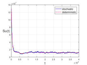
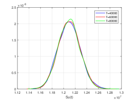
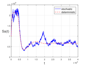
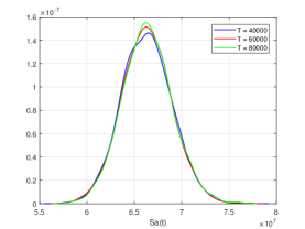
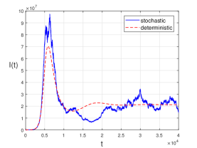
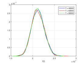
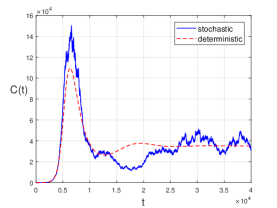
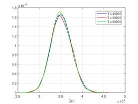
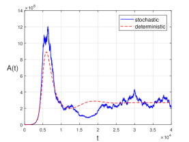
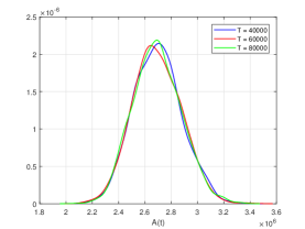
Figure 6.1 The persistence and stationary distribution of $S_{u},S_{a},I,C,A$ in model (2.3)

We set $\beta=\frac{0.1065}{229800000}$ and keep the remaining parameters and initial values same with those in Figure 6.1. So, $\hat{R}_{0}^{e}\approx 0.0229<1$ and

$$0.0148\approx\mu>0.5(\sigma_{1}^{2}\vee\sigma_{2}^{2}\vee\sigma_{3}^{2}\vee\sigma_{4}^{2}\vee\sigma_{5}^{2})=0.00125.$$

By Theorem 5.1, HIV/AIDS is extinct in Figure 6.2.

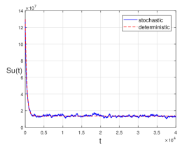
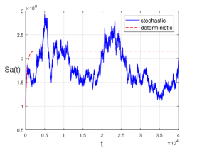
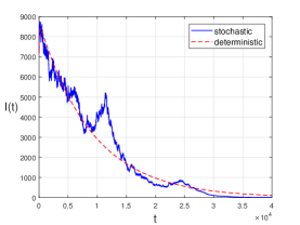
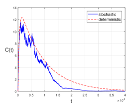
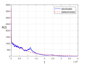
Figure 6.2 The extinction of HIV/AIDS

Next, we discuss the impacts of the parameter $\varepsilon$, and let $\sigma_{i}(i=1,2,3,4,5)\\ =0.02$ and other parameters and the initial values be same with those in Figure 6.1. We observe that HIV/AIDS is persistent as $\varepsilon$ increases, while the population size of the infected decreases significantly in Figure 6.2 Therefore, the enhancement of $\varepsilon$ is of significant importance for the prevention and control of HIV/AIDS.

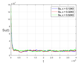
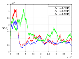
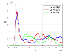
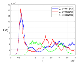
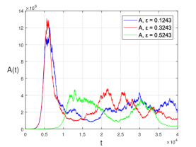
Figure 6.3 The impact of $\varepsilon$

Example 6.2.

We perform the numerical simulations on the spread of HIV/AIDS in China for next five decades, and provide some suggestions for the epidemics in this example. Since the population size for the year 2014 was 1376460000 in China, and the average life span of the population was 76.34 ref32 , we assume that the natural growth rate, the natural mortality rate and the infection rate for the population are respectively

$$\lambda=\frac{1376460000}{76.34},\mu=\frac{1}{76.34},\beta=\frac{0.71}{1376460000}.$$

By the data in 2014 in Zhao et al.ref29 , the number of the individuals with HIV/AIDS was 500579, and the number of the individuals with ART was 295358, therefore we assume that

$$S_{u}=1088230000,S_{a}=288230000,I=153193,C=295358,A=52128$$

and choose $\Delta=10^{-2}$ and $\alpha=0.13,\varepsilon=0.5,\eta=0.18,\upsilon=0.72,\gamma=0.14,\rho=0.82,\delta=0.42$ as other parameters for simulation.

Firstly, we collect the data for the individuals with HIV/AIDS from the year 2014 to 2020 in China in Zhao et al.ref29 (year 2014-2018), Liu et al.ref30 (year 2019) and He ref31 (year 2020). We thus adopt Runge Kutta method to fit the parameters, and the simulation with fitted parameters and the data are shown on the left of Figure 6.4. By Theorem 4.1, we derive that $R_{0}^{s}=2.8942>1$ as $\sigma_{i}=0.05(i=1,2,3,4,5)$. Further, we govern the data in 2020 as the initial values to preform the simulations for next 5 decades in China as presented on the right of Figure 6.4. It is easy to observe that although the spread of HIV/AIDS in China is running in a low epidemic level, there still exists a risk of the exponential growth for HIV/AIDS control.

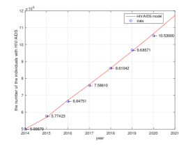
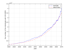
Figure 6.4 Data fitting for the individuals with HIV/AIDS from 2014 to 2022, and prediction of HIV/AIDS for next 5 decades in China

Next, we discuss the impacts of main parameters to the control of HIV/ AIDS in China. The extensive publicity and detailed publicity on HIV/AIDS are two important ways to prevent and control the spread of HIV/AIDS in China. In practice, the extensive publicity improves the number of the individuals having protection awareness from $S_{u}$ to $S_{a}$ by varying $\alpha$, which further reveals that less impact on the transmission of HIV/AIDS occurs as $\alpha$ increases (see the left in Figure 6.5). Meanwhile, the detailed publicity presents more details for the individuals who are infected by HIV, and the isolations within 72 hours are usually adopted to reduce the infection rates, which further suppresses the number of the individuals with HIV/AIDS as $\varepsilon$ increases (see the right in Figure 6.5).

Therefore, the extensive publicity and the detailed publicity including lessons and lectures of AIDS in universities and communities to the target population play significant roles to prevent the spread of HIV/AIDS.

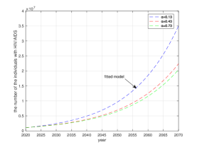
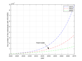
Figure 6.5 Impacts of the extensive publicity and detailed publicity on HIV/AIDS

The prompt and continuous antiretroviral therapy (ART) after being infected is helpful to each individual with HIV/AIDS. Figure 6.6 demonstrates the simulations with distinct values of $\eta$, which also verify that ART suppresses the rapid growth of the individuals who are with HIV/AIDS as $\eta=0.08$.

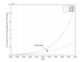
Figure 6.6 Impact of the continuous ART

We also notice that the transmission rates $\gamma$ and $v$ affect the long-term epidemics of HIV/AIDS in China. More precisely, when $\gamma$ increases (also the period that the individuals with HIV/AIDS see the doctors in hospital and get checked becomes shorter), the number of the individuals with HIV/AIDS decrease. Meanwhile, when $v$ increases (also the period that the individuals with AIDS stay at hospital becomes shorter), the number of the individuals with HIV increases as presented in Figure 6.7.

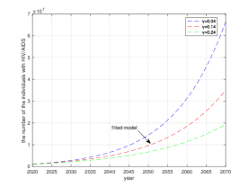
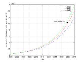
Figure 6.7 Impacts of $\gamma$ and $v$ on HIV/AIDS

7 Conclusions and discussions

We propose a stochastic epidemic model with the bilinear incidence rate and show that the existence of a global positive solution. By constructing Lyapunov functions, we also show that the stochastic model has an ergodic stationary distribution when $R^{s}_{0}>1$. Moreover, the sufficient condition $R^{e}_{0}<1$ for the extinction of HIV/AIDS is obtained. The corresponding simulations verify that the numbers of the individuals in Indonesia and in China decreas when the detailed publicity and the continuous ART are governed to prevent and control the spread of HIV/AIDS. Therefore, we suggest that all countries should enhance the systematic and detailed publicity on AIDS, which are of significant importance to control the growth of HIV/AIDS. For instance, taking the isolations within 72 hours and receiving prompt ART treatment after being infected are the effective measurements for the elimination of AIDS by 2030.

Compared with the conclusions derived by Fatmawati et al. ref5 , the disease-free equilibrium point $P_{0}$ attracts the solution of (2.3) under condition $R_{0}^{e}<1$ (see Theorem 5.1), which also means that HIV/AIDS becomes extinct as the intensities of the white noises increase. Meanwhile, the solution of (2.3) fluctuates around the endemic equilibrium $P^{*}$, and the solution has a unique ergodic stationary distribution when $R_{0}^{s}>1$ (see Theorem 4.1).

We also point out that the expressions for $R_{0}^{s}$ and $R_{0}^{e}$ are two distinct indices for indicating the prevalence of HIV/AIDS. When the intensities of the white noises disappear, $R_{0}^{s}$ turns into $R_{0}$ in (2.2). Theoretically, model (2.3) has a smaller index for the persistence of HIV/AIDS than that of model (2.1). The long-term properties of model (2.3) are quite different from the results in Fatmawati et al. ref5 .

Conflict of interest

All authors consent to publish the main results of this paper on Journal of Dynamics and Differential Equations. All authors declared that we did not and do not have any conflicts of interest with any other institutions and groups.

References

• (1) Tunstall-Pedoe, H.: Preventing Chronic Diseases: a Vital Investment: WHO Global Report. International Journal of Epidemiology. 35(4), 1107-1107 (2005)
• (2) WHO, https://www.who.int/news-room/fact-sheets/detail/hiv-aids
• (3) Silva, C. J., Torres, D. F.: A SICA compartmental model in epidemiology with application to HIV/AIDS in Cape Verde. Ecological complexity. 30, 70-75 (2017)
• (4) Ghosh, I., Tiwari, P. K., Samanta, S., Elmojtaba, I. M., Al-Salti, N., Chattopadhyay, J.: A simple SI-type model for HIV/AIDS with media and self-imposed psychological fear. Mathematical Biosciences. 306, 160-169 (2018)
• (5) Fatmawati, Khan, M. A., Odinsyah, H. P.: Fractional model of HIV transmission with awareness effect. Chaos, Solitons & Fractals. 138, 109967 (2020)
• (6) Zhao, Y., Elattar, E. E., Khan, M. A., Fatmawati, Asiri, M., Sunthrayuth, P.: The dynamics of the HIV/AIDS infection in the framework of piecewise fractional differential equation. Results in Physics, 40, 105842 (2022)
• (7) Mao, X., Marion, G., Renshaw, E.: Environmental Brownian noise suppresses explosions in population dynamics. Stochastic Processes and their Applications. 97(1), 95-110 (2002)
• (8) Liu, H., Yang, Q., Jiang, D.: The asymptotic behavior of stochastically perturbed DI SIR epidemic models with saturated incidences. Automatica. 48(5), 820-825 (2012)
• (9) Witbooi, P. J.: Stability of an SEIR epidemic model with independent stochastic perturbations. Physica A: Statistical Mechanics and its Applications. 392(20), 4928-4936 (2013)
• (10) Liu, H., Yang, Q., Jiang, D.: The asymptotic behavior of stochastically perturbed DI SIR epidemic models with saturated incidences. Automatica. 48(5), 820-825 (2012)
• (11) Wei, F., Chen, F.: Stochastic permanence of an SIQS epidemic model with saturated incidence and independent random perturbations. Physica A: Statistical Mechanics and its Applications. 453, 99-107 (2016)
• (12) Lu, R., Wei, F.: Persistence and extinction for an age-structured stochastic SVIR epidemic model with generalized nonlinear incidence rate. Physica A: Statistical Mechanics and its Applications. 513, 572-587 (2019)
• (13) Wei, F., Xue, R.: Stability and extinction of SEIR epidemic models with generalized nonlinear incidence. Mathematics and Computers in Simulation. 170, 1-15 (2020)
• (14) Liu, Q., Jiang, D., Hayat, T., Alsaedi, A.: Stationary distribution and extinction of a stochastic HIV-1 infection model with distributed delay and logistic growth. J. Nonlinear Sci. 30(1), 369-395 (2020)
• (15) Qi, K. Jiang, D.: The impact of virus carrier screening and actively seeking treatment on dynamical behavior of a stochastic HIV/AIDS infection model. Applied Mathematical Modelling. 85, 378-404 (2020)
• (16) Liu, Q.: Dynamics of a stochastic SICA epidemic model for HIV transmission with higher-order perturbation. Stochastic Analysis and Applications. 2021,1-40 (2021)
• (17) Wang, X., Wang, C., Wang, K.:Extinction and persistence of a stochastic SICA epidemic model with standard incidence rate for HIV transmission. Advances in Difference Equations. 2021, 260 (2021)
• (18) Djordjevic, J., Silva, C. J., Torres, D. F.: A stochastic SICA epidemic model for HIV transmission. Applied Mathematics Letters. 84, 168-175 (2018)
• (19) Wang, Y., Jiang, D., Alsaedi, A., Hayat, T.: Modelling a stochastic HIV model with logistic target cell growth and nonlinear immune response function. Physica A: Statistical Mechanics and its Applications. 501, 276-292 (2018)
• (20) Wei, F., Liu, J.: Long-time behavior of a stochastic epidemic model with varying population size. Physica A: Statistical Mechanics and Its Applications. 470, 146-153 (2017)
• (21) Wei, F., Jiang, H., Zhu, Q.: Dynamical behaviors of a heroin population model with standard incidence rates between distinct patches. Journal of the Franklin Institute. 358(9), 4994-5013 (2021)
• (22) Diekmann, O., Heesterbeek, J. A. P., Metz, J. A. P.: On the Definition and Computation of the basic reproduction ratio R0 in the model of infectious diseases in heterogeneous populations J. Math. Biol. 28, 365-382 (1990)
• (23) Van den Driessche, P., Watmough, J.: Reproduction numbers and sub-threshold endemic equilibria for compartmental models of disease transmission. Mathematical biosciences. 180(1-2), 29-48 (2002)
• (24) Imhof, L., Walcher, S.: Exclusion and persistence in deterministic and stochastic chemostat models. Journal of Differential Equations. 217(1), 26-53 (2005)
• (25) Liu, Q., Jiang, D., Shi, N., Hayat, T., Alsaedi, A.: Stationarity and periodicity of positive solutions to stochastic SEIR epidemic models with distributed delay. Discrete & Continuous Dynamical Systems-B. 22(6), 2479-2500 (2017)
• (26) Wang, L., Jiang, D.: A note on the stationary distribution of the stochastic chemostat model with general response functions. Applied Mathematics Letters. 73, 22-28 (2017)
• (27) Dalal, N., Greenhalgh, D., Mao, X.: A stochastic model for internal HIV dynamics. Journal of Mathematical Analysis and Applications. 341(2), 1084-1101 (2008)
• (28) Wang, L., Jiang, D.: Ergodic property of the chemostat: A stochastic model under regime switching and with general response function. Nonlinear Analysis: Hybrid Systems. 27, 341-352 (2018)
• (29) Evans, S.N., Ralph, P.L., Schreiber, S.J., Arnab, S.: Stochastic population growth in spatially heterogeneous environments. J. Math. Biol. 66, 423-476 (2013)
• (30) Tan, Y., Cai, Y., Sun, X., Wang, K., Yao, R., Wang, W., Peng, Z.: A stochastic SICA model for HIV/AIDS transmission. Chaos, Solitons & Fractals. 165, 112768 (2022)
• (31) Khasminskii, R.: Stochastic Stability of Differential Equations. Springer, Berlin, Heidelberg Publishing (1980)
• (32) Zhao, Y., Jiang, D.: The threshold of a stochastic SIS epidemic model with vaccination. Applied Mathematics and Computation. 243, 718-727 (2014)
• (33) Mao, X., Wei, F., Wiriyakraikul, T.: Positivity preserving truncated Euler-Maruyama Method for stochastic Lotka-Volterra competition model. Journal of Computational and Applied Mathematics. 394, 113566 (2021)
• (34) Zhao, Y. Han, M. Ma, Y. Li, D.: Progress Towards the 90-90-90 Targets for Controlling HIV — China. China CDC Weekly. 1(1), 4-7 (2019)
• (35) Liu, E. Wang, Q. Zhang, G. Chen, M.: Tuberculosis/HIV Coinfection and Treatment Trends - China. China CDC Weekly. 2(48), 924-928 (2020)
• (36) He, N.: Research Progress in the Epidemiology of HIV/AIDS in China. China CDC weekly. 3(48), 1022-1030 (2021)
• (37) NBS, https://data.stats.gov.cn/english/easyquery.htm?cn=C01