FusionFormer: Fusing Operations in Transformer for Efficient Streaming Speech Recognition

Xingchen Song^1,2,3,, Di Wu^2,3,∗, Binbin Zhang^2,3, Zhiyong Wu¹, Wenpeng Li², Dongfang Li²
Pengshen Zhang², Zhendong Peng^2,3, Fuping Pan², Changbao Zhu² Zhongqin Wu²
¹ Tsinghua University, Beijing, China ² Horizon Robtics, Beijing, China
³ WeNet Open Source Community
sxc19@mails.tsinghua.edu.cn Equal Contribution and Corresponding Author.

Abstract

The recently proposed Conformer architecture which combines convolution with attention to capture both local and global dependencies has become the de facto backbone model for Automatic Speech Recognition (ASR). Inherited from the Natural Language Processing (NLP) tasks, the architecture takes Layer Normalization (LN) as a default normalization technique. However, through a series of systematic studies, we find that LN might take 10% of the inference time despite that it only contributes to 0.1% of the FLOPs. This motivates us to replace LN with other normalization techniques, e.g., Batch Normalization (BN), to speed up inference with the help of operator fusion methods and the avoidance of calculating the mean and variance statistics during inference. After examining several plain attempts which directly remove all LN layers or replace them with BN in the same place, we find that the divergence issue is mainly caused by the unstable layer output. We therefore propose to append a BN layer to each linear or convolution layer where stabilized training results are observed. We also propose to simplify the activations in Conformer, such as Swish and GLU, by replacing them with ReLU. All these exchanged modules can be fused into the weights of the adjacent linear/convolution layers and hence have zero inference cost. Therefore, we name it FusionFormer. Our experiments indicate that FusionFormer is as effective as the LN-based Conformer and is about 10% faster.

1 Introduction

End-to-End Automatic Speech Recognition (ASR) has become the standard of state-of-the-art approaches (Li, 2021). While recurrent neural networks (RNN) (Graves et al., 2013; Chan et al., 2016) have drawn attention as popular backbone architectures for ASR models to generate acoustic representations (encoding) and predict characters at different time steps (decoding), The recurrent nature of RNN limits the parallelization of computation and it becomes especially severe for speech recognition task since speech sequences are commonly long. To overcome these shortcomings, (Dong et al., 2018) introduced the Transformer (Vaswani et al., 2017) to ASR task, which achieved better performance with markedly less training cost and no-recurrence. The fundamental module of Transformer is self-attention that relates all the position-pairs of a sequence to generate a more expressive sequence representation. Since the self-attention dose not involve local context whereas Convolutional Neural Networks (CNN) are good at modeling such information, (Gulati et al., 2020) proposed to augment the Transformer network with convolution to model both local and global dependencies. This novel convolution-augmented Transformer architecture, called Conformer, has become the de facto model for ASR tasks due to its ability to capture global and local features synchronously from audio signals (Li, 2021). It has also achieved state-of-the-art performance in combination with recent developments in various end-to-end speech processing tasks as well (Guo et al., 2021).

Indeed the availability of sufficient training resources and large scale hand-labeled datasets made it possible to train powerful deep neural network, i.e., Conformer, for ASR to reach very low Word Error Rate (WER) and break state-of-the-art results. One major drawback for using Conformer in real-world is the inference resource cost, especially for edge-devices that are widely used in production environment (Burchi and Vielzeuf, 2021). More fundamentally, this raises the question of whether there has room for optimizing Conformer and achieving comparative performance in ASR tasks.

Refer to caption — (a) Parameters of model (M)

In literature, many studies on efficient neural networks have just emerged in the past year (Menghani, 2021) and different approaches have been proposed to address the problem of integrating neural networks as a production-ready technology. Those approaches may be gathered into several broad categories (Han et al., 2016), such as quantization (Guo, 2018), weights sharing (Dabre and Fujita, 2019), pruning (Molchanov et al., 2017), efficient architecture design (Tan and Le, 2019) and low-rank decomposition (Cheng et al., 2018). All these methods may help to reduce the computation requirements. In this paper, we choose to focus on the design of an efficient architecture to address the ASR problem.

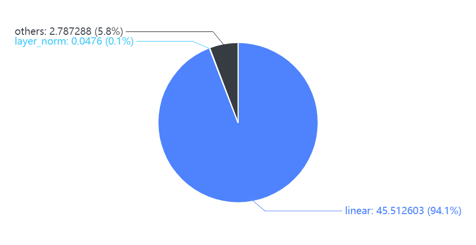
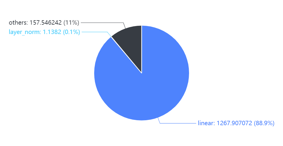
Empirically, we perform a careful and systematic analysis of the theoretical computation overhead (i.e., parameters or FLOPs) and the real-world inference latency for Conformer (see Figure 2) and find that the most valuable optimization for Conformer could be removing Layer Normalizations (Ba et al., 2016). Based on our analysis, we first perform two direct applications of using BN instead of LN or simply exclude all LN. All these changes however result in frequent divergence in model training. To investigate this phenomenon, we proposed Layer Trend Plots (LTPs) to adapt the difference of statistics calculation between standard Conformer and its variants. Then we monitor the LTPs during training and find that most of such divergences are due to the unstable layer output. We thus propose to append a BN layer to each linear or convolution layer. The effectiveness of this simple modification is proved not only by observed stabilized training (Table 4) but also the on-par results with LN-based Conformer on ASR tasks (Table 2). Besides, ascribed to the use of BN, our FusionFormer easily acquire 10% speed performance gain without any special optimizations.

2 Methodology

We describe the exploration of LN-free Conformer design space in this section. First, we discuss the relationships of various techniques to achieve streaming Conformer and perform a systematic analysis of how steaming Conformer spends its time. Then we conduct two straightforward experiments to optimize the Conformer model and find that all these plain attempts lead to divergence. Finally we use our proposed Layer Trend Plots (LTPs) to analyze the reasons for the divergence of the above initial attempts and propose a solution to build a robust LN-free Conformer.

2.1 Streaming Conformer

In this paper, we mainly focus on streaming speech recognition. Streaming ASR is an important scenario in online application. It emits tokens as soon as possible after receiving a partial utterance from the speaker. However, the insufficient future context may lead to performance degradation and there exists a trade-off between latency and accuracy (Chen et al., 2021). The original Attention-based Encoder-Decoder (AED) model, i.e. Transformer or Conformer, for ASR are not streaming in nature by default, as the global attention mechanism requires all input feature sequence for the calculation of monotonic attention alignment to generate context information. To address streaming issues for AED, several methods have been proposed:

1.

Chunk-wise methods (Tian et al., 2020; Wang et al., 2020) segment the input into small chunks and recognize on each chunk individually.
2.

Memory based methods (Wu et al., 2020; Inaguma et al., 2020) introduce a contextual vector to encode history information.
3.

Time-restricted methods (Yu et al., 2020; Tripathi et al., 2020) control time cost by simply masking left and right context in Transformer.

All these existing methods have their own drawbacks. For chunk-wise methods, the accuracy drops significantly as the relationship between different chunks are ignored. For memory based methods, they break the parallel nature of Transformer in training, requiring a longer training time. For time-restricted methods, a large latency is introduced as the reception field grows linearly with the number of Transformer layers. To overcome these shortcomings and reach a balance between training cost, runtime cost, and accuracy, (Wu et al., 2021) combines chunk-wise processing and time-restricted context to handle streaming scenario, where audio signals are truncated into several segments and processed chunk by chunk with the accessibility to previous chunks to model relationships between chunks. Besides, to guarantee the training efficiency, there is no overlap between chunks in training. In order to conduct efficient decoding for the proposed streaming Conformer (called U2++), (Wu et al., 2021) also implemented an efficient decoder based on beam search with C++, coupled with a high-performance WebSocket server specially tailored for U2++ and can be used in real production environment³³3https://github.com/wenet-e2e/wenet. Due to its state-of-the-art accuracy, open sourced reproducibility and widespread adoption by industry, we choose U2++ in (Wu et al., 2021) as our baseline streaming Conformer and profile it in the next subsection.

2.2 Is There Any Room for Optimizing Streaming Conformer?

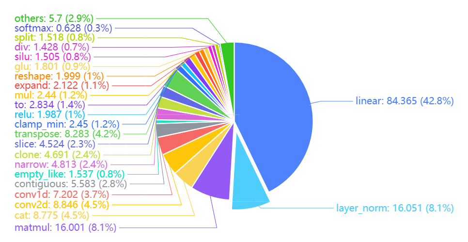
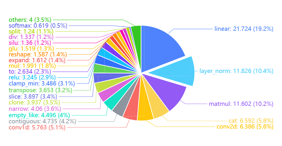
In Figure 2, we show the breakdown of parameters, floating-point operations per second (FLOPs) and latency among the main components of the Conformer network (see Figure 3). We observe that calculations in the Layer Normalization modules account for only 0.1% of the total parameters and FLOPs. However, they account for 8.1% and 10.4% of the latency in float32 inference and int8 inference, respectively. Given that huge gap between FLOPs and latency, it’s nature to turn our focus to removing the Layer Normalizations since it allows us to get the maximum benefit at the minimum cost.

2.3 Initial Attempts

As for initial attempts, we conduct two straightforward experiments by:

1.

Simply removing all LN layers (denoted as Conformer-NoNorm).
2.

Directly replacing all LN layers by BN layers at the same place (denoted as Conformer-BN).

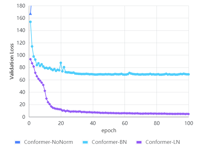
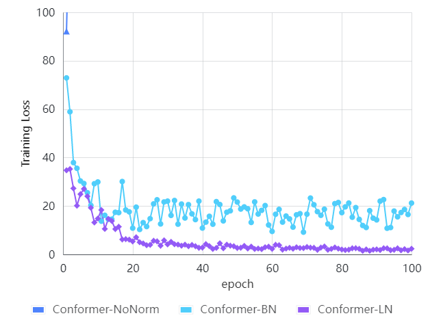
Our model is based on standard version of U2++ Conformer (denoted as Conformer-LN), and all the other hyperparameters follow the settings in Appendix A.3. Unexpectedly, these plain designs lead to convergence problems, i.e., the model is very unstable to frequently crash during early-stage training or unable to exceed the current local optima. The validation and training curves in Figure 2 with three different models reveal that LN plays an important role to stabilize the training of Conformer and we have to dig out how LN works. We hypothesize these divergences are originated from unstable layers, which may be observed with some abnormal statistics in the hidden outputs.

2.4 Analysis

The recently proposed Signal Propagation Plots (SPPs) (Brock et al., 2021) are proved to be helpful to find out the key reason that contributing to model divergence. SPPs are originally designed for deep ResNets where the statistics of the hidden activations, i.e., the activations of each residual block before training, are used as a simple set of visualizations. We notice that although SPPs theoretically analyzed signal propagation in ResNets, it is a static analysis of a randomly initialized model and we find that practitioners rarely empirically evaluate the scales of different layer outputs across different training times when designing new models or proposing modifications to existing architectures. By contrast, we found that plotting the dynamic statistics of the layer outputs at different training steps on a batch of either real training examples or random Gaussian inputs, can be extremely beneficial. This practice not only allows us to identify special phenomena which might be challenging to derive from scratch, but also enables us to immediately detect hidden bugs in our plain implementations. To formalize this good practice, we propose Layer Trend Plots (LTPs), a simple graphical method for visualizing layer behaviours across training stage on the forward pass in Conformer.

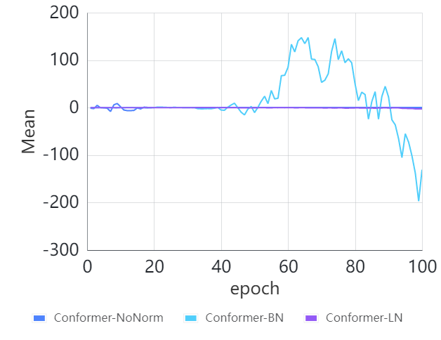
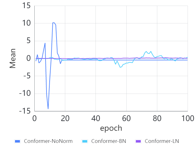
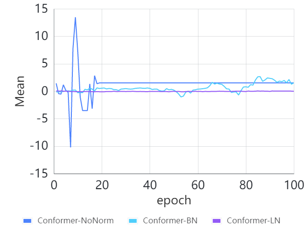
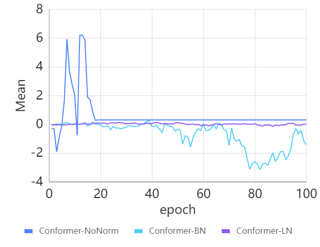
To monitor the trend of layer output, we plot the following statistics for every layer in Conformer:

1.

Mean, computed as the average value of the layer output.
2.

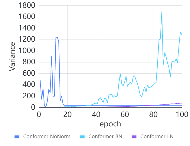
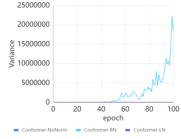
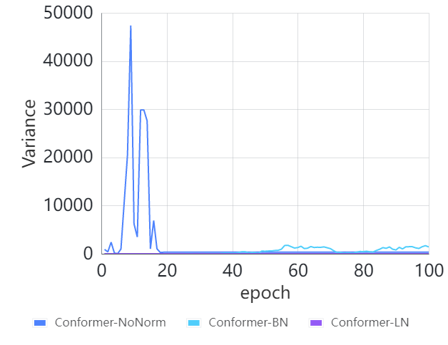
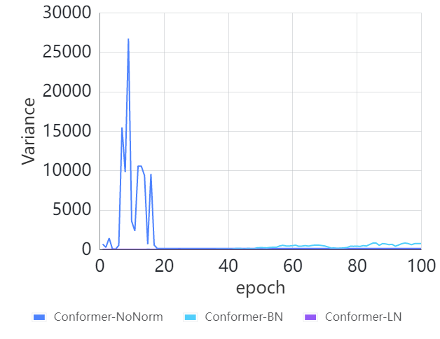
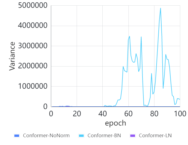
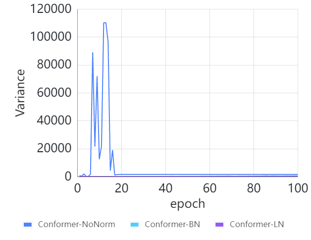
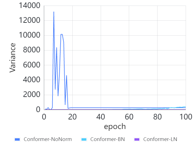
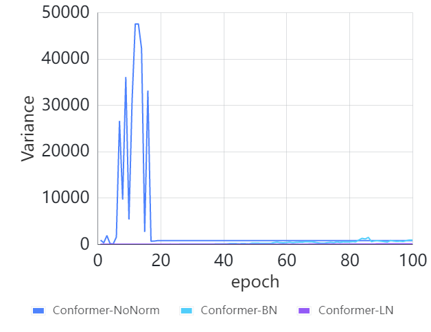
Variance, computed as the variance of all elements in the layer output.

Model	Architecture	Hidden	Heads	Params (M)
12CE + 6CD	12 Conformer Encoder + 6 Conformer Decoder	256	4	48
12FE + 6CD	12 FusionFormer Encoder + 6 Conformer Decoder	256	4	48
12FE + 6FD	12 FusionFormer Encoder + 6 FusionFormer Decoder	256	4	48
16CE + 6CD	16 Conformer Encoder + 6 Conformer Decoder	384	6	98
16FE + 6CD	16 FusionFormer Encoder + 6 Conformer Decoder	384	6	98
16FE + 6FD	16 FusionFormer Encoder + 6 FusionFormer Decoder	384	6	98

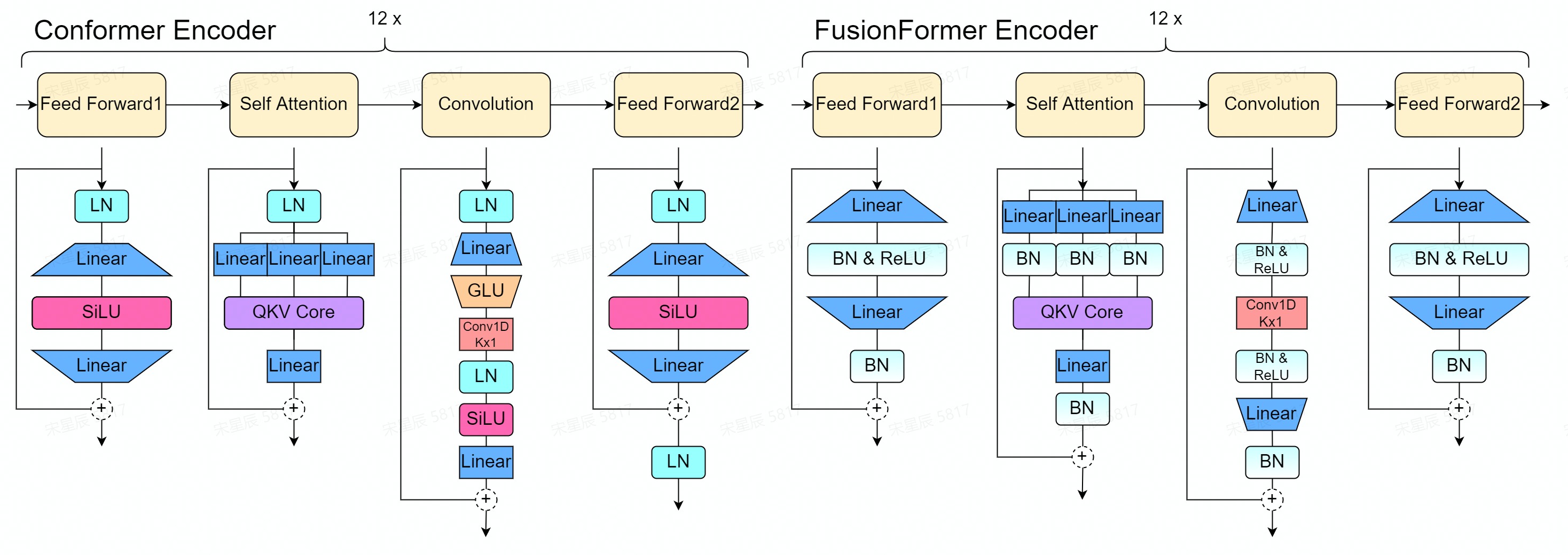
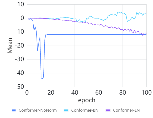
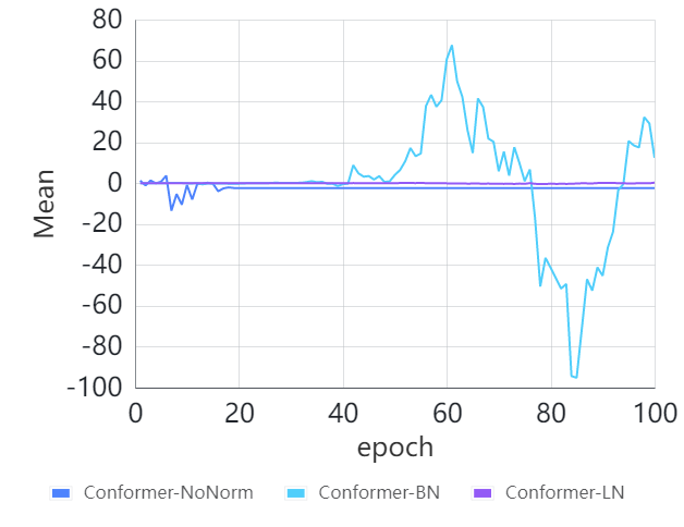
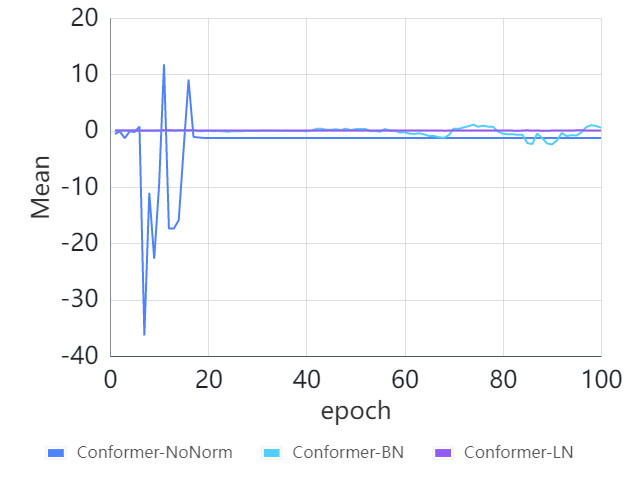
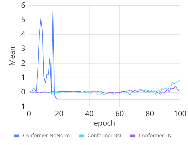
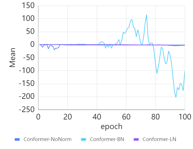
Table 1: Detailed architecture configurations for Conformer and FusionFormer.

We generally find these statistics to be informative measure of the training magnitude, and to clearly show explosion or attenuation. To generate LTPs, we provide the network with a batch of input examples sampled from a standard normal distribution. We also experiment with feeding real data samples instead of random noise and find this does not affect the key trends. With LTPs, we observe several meaningful patterns as plotted in Appendix A.1 and Figure 4, where the y-axis denotes the values of corresponding statistics, and the x-axis denotes the index of the training epochs. For Conformer, there are 11 linear/convolution layers for each block, while detailed position of each layer can be found in Figure 3.

First, we find that most of the layers in Conformer-NoNorm changed rapidly and abnormally at the very beginning of training, which is consistent with our observation in Figure 2 that the model will face crash problems at early stage. Second, different from Conformer-NoNorm, models with normalization such as Conformer-BN and Conformer-LN have controllable statistics at beginning. However, Conformer-BN may suffer from “layer crash” at the later training stages, especially for layers in Feed Forward and Self Attention. These patterns are double-checked in LTPs of Variance and we show them in Appendix A.1 and Figure 5.

2.5 Solutions

Based on our observations in section 2.4, we argue that the convergence problem is mainly contributed to the unstable Mean and Variance of layer output and putting normalization in appropriate position can alleviate this problem to a certain extent, i.e., by placing LN at each residual branch like what standard Conformer has done or simply appending BN to each linear/convolution layer. We therefore propose our solution in the right part of Figure 3, where LN is removed and BN is added after each layer. Besides stabilizing the layer output, another advantage of appending BN is that we can fuse BN into preceding linear/convolution layers which is a quite mature technique for speedup (Duan et al., 2018). We can never do similar things for LN since LN needs to calculate the mean and variance statistics during inference while BN does not (Yao et al., 2021).

We also propose to simplify the activation in Conformer for extra speedup. In the left part of Figure 3, Conformer uses Swish activation (also known as SiLU) for most of the modules. However, it switches to a Gated Linear Unit (GLU) for its convolution module. Such a heterogeneous design seems over-complicated and quantization-unfriendly (Kim et al., 2022). From a practical view, multiple activations complicates hardware deployment, as an efficient implementation of int8 activation requires custom approximations or look up tables (Kim et al., 2021; Yu et al., 2021). To address this, we propose to replace the GLU and Swish activation with ReLU (Agarap, 2018), unifying the choice of activation function throughout the entire model. We note that ReLU can also be fused into the previous layers (Stevewhims, 2021).

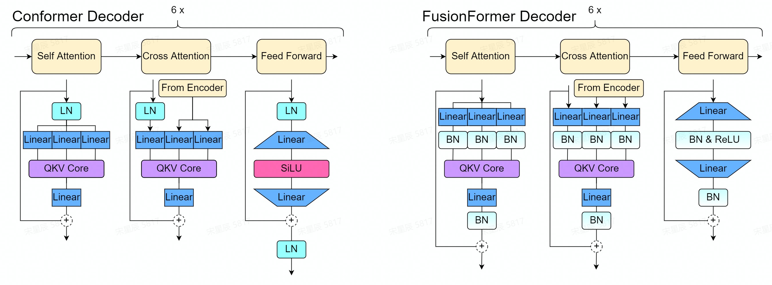
Since Conformer decoder only contains Feed Forward and Attention modules, it is simple and straightforward to apply similar modifications to decoder, detailed structures of decoder can be seen in Appendix A.2.

Model	1st-s-16-4	1st-s-16- $\infty$	1st-ns- $\infty$ - $\infty$	2nd-s-16-4	2nd-s-16- $\infty$	2nd-ns- $\infty$ - $\infty$
12CE + 6CD	6.15	5.96	5.33	5.12	5.09	4.72
12FE + 6CD	6.39	6.30	6.01	5.31	5.27	4.97
12FE + 6FD	6.43	6.35	5.83	5.32	5.27	4.98
16CE + 6CD	5.90	5.87	5.26	5.09	5.00	4.68
16FE + 6CD	6.17	6.08	5.54	5.19	5.10	4.82
16FE + 6FD	6.12	6.05	5.63	5.22	5.12	4.85

Table 2: WER (%) Comparison of different models with different decoding methods on AISHELL-1.

Model	Decoding Method	WER	Correct	Substitute	Delete	Insert
12CE + 6CD	1st-s-16-4	6.15	98429	6139	197	107
	1st-s-16- $\infty$	5.96	98633	5975	157	110
	1st-ns- $\infty$ - $\infty$	5.33	99290	5349	126	104
	2nd-s-16-4	5.12	99500	5128	137	101
	2nd-s-16- $\infty$	5.09	99529	5096	140	98
	2nd-ns- $\infty$ - $\infty$	4.72	99914	4730	121	93
12FE + 6CD	1st-s-16-4	6.39	98183	6407	175	112
	1st-s-16- $\infty$	6.30	98264	6328	173	103
	1st-ns- $\infty$ - $\infty$	6.01	98760	5839	166	294
	2nd-s-16-4	5.31	99299	5302	164	92
	2nd-s-16- $\infty$	5.27	99327	5278	160	83
	2nd-ns- $\infty$ - $\infty$	4.97	99635	4972	158	79
12FE + 6FD	1st-s-16-4	6.43	98132	6457	176	107
	1st-s-16- $\infty$	6.35	98213	6380	172	103
	1st-ns- $\infty$ - $\infty$	5.83	98756	5853	156	103
	2nd-s-16-4	5.32	99287	5314	164	97
	2nd-s-16- $\infty$	5.27	99335	5269	161	87
	2nd-ns- $\infty$ - $\infty$	4.98	99633	4975	157	88

Table 3: WER (%) comparison of different models with different decoding methods on AISHELL-1, including all kinds of misrecognitions.

It is well known that fewer layers means faster speed and less quantization accuracy loss (Guo, 2018). With all the above optimizations, we get a new architecture called FusionFormer, which is speed-oriented and quantization-friendly.

3 Experiments

Models. Following the architecture described in (Wu et al., 2021), we construct standard U2++ Conformer with 12 encoder blocks and 6 decoder blocks and scale it up to 16 encoder blocks. In particular, we apply the proposed architecture changes in Section 2.5 to construct FusionFormer from Conformer, retaining the model size. Detailed architecture configurations are described in Table 1.

Training Details. Because the training recipes and codes for Conformer have been fully open-sourced⁴⁴4https://github.com/wenet-e2e/wenet/blob/main/examples/aishell/s0/conf, we strictly follow the settings except that we use dynamic left chunks to simulate different context for streaming decoding. We train both Conformer and FusionFormer on a public Mandarin speech corpus, named AISHELL-1 (Bu et al., 2017), for 700 epochs on 4 GeForce-RTX-3090, More details for the training setup are given in Appendix A.3.

Decoding Method	lr=0.003	lr=0.0025	lr=0.002	lr=0.0015	lr=0.001*	lr=0.0005
1st-s-16-4	6.50	6.46	6.43	6.53	6.61	6.68
1st-s-16- $\infty$	6.38	6.43	6.35	6.43	6.53	6.64
1st-ns- $\infty$ - $\infty$	5.89	5.88	5.83	5.90	6.06	6.21
2nd-s-16-4	5.34	5.37	5.32	5.40	5.42	5.48
2nd-s-16- $\infty$	5.27	5.34	5.27	5.29	5.35	5.44
2nd-ns- $\infty$ - $\infty$	4.98	5.07	4.98	5.01	5.10	5.16

Table 4: Analysis on different learning rate for different decoding methods. Experiments are conducted with 12FE + 6FD. We find that FusionFormer is trained smoothly without any crashes and is extremely robust to learning rate (lr). * indicates the best setting for LN-based model, it’s also the default setting for training our Conformer-LN baseline.

Decoding Methods. U2++ supports two-pass decoding where encoder is used to generate n-best hypotheses, either in a streaming manner or in a non-streaming manner, for the first pass and the hypotheses are then rescored by the decoder to get the second pass result. We therefore get 6 different decoding configurations:

1.

1st-s-16-4: First pass streaming result with chunksize=16 and accessibility to previous 4 chunks.
2.

1st-s-16- $\infty$ : First pass streaming result with chunksize=16 and accessibility to all previous chunks.
3.

1st-ns- $\infty$ - $\infty$ : First pass non-streaming result with chunksize= $\infty$ , it is equal to standard offline speech recognition.
4.

2nd-s-16-4: Second pass streaming result with chunksize=16 and accessibility to previous 4 chunks.
5.

2nd-s-16- $\infty$ : Second pass streaming result with chunksize=16 and accessibility to all previous chunks.
6.

2nd-ns- $\infty$ - $\infty$ : Second pass non-streaming result with chunksize= $\infty$ , it is equal to standard offline speech recognition.

3.1 Main Results

We use Word Error Rate (WER) as metric and the main results are shown in Table 2.

Conformer Encoder vs. FusionFormer Encoder. Compared to the LN-based Conformer (12CE + 6CD), BN-based FusionFormer (12FE + 6CD) suffers a significant drop in first pass decoding (6.15 / 5.96 / 5.33 vs. 6.39 / 6.30 / 6.01). We additionally check all types of misrecognitions in Table 3, and find that this gap is mainly due to higher substitution errors (6139 / 5975 / 5349 vs. 6407 / 6328 / 5839). However, after the second pass decoding, this situation is mitigated (5.12 / 5.09 / 4.72 vs. 5.31 / 5.27 / 4.97 and 5128 / 5096 / 4730 vs. 5302 / 5278 / 4972). Considering the initial divergence, these comparable results demonstrate the practicality of LTPs and the reliability of the proposed modifications.

Conformer Decoder vs. FusionFormer Decoder. To verify our proposed method works equally well for the decoder, we also evaluate the performance of FusionFormer Encoder + FusionFormer Decoder. By comparing 12FE + 6CD and 12FE + 6FD, we can clearly see that our methods generalize well on Decoder since WER is almost the same.

Deeper Conformer vs. Deeper FusionFormer. As shown in the last three lines of Table 2, our architecture scales well to larger models and consistently achieves the on-par results with LN-based counterparts.

3.2 Further Analysis

Stability. To validate our conjecture in Section 2.5 that the convergence problem is mainly caused by the unstable Mean and Variance of layer output and putting normalization in appropriate position can alleviate this problem, we present some WER comparisons with different hyper-parameter setups in Table 4. It is well known that Self Attentions are very sensitive to hyper-parameters, especially to learning rate (Popel and Bojar, 2018). Therefore, huge efforts have to be devoted to hyper-parameter tuning. However, by applying our proposed modifications which append BN to each convolution/linear layers and simplify activation functions, there is no more crashes and the performance is much more stable. Besides, the results also suggest that it’s better to use a higher learning rate (lr) when training our proposed FusionFormer while the optimal learning rate for Conformer is smaller.

Speed. Run Time Factor (RTF) is obtained by calculating the ratio of the total decoding time to the total audio time and is widely adopted as a model-level end-to-end speed metric in ASR. We run tests on AISHELL-1 testset for both Conformer and FusionFormer to evaluate the speed performance. As Table 5 shows, by fusing operations such as BN and ReLU into previous layers, the inference speed of FusionFormer consistently outperforms Conformer and achieves over 10% speedup, without noticeable WER changes.

Model	RTF(float32)	RTF(int8)
12CE + 6CD	0.1053	0.07064
12FE + 6FD	0.08962	0.06047

Table 5: RTF comparison of different model with decoding method 2nd-s-16-

\infty

. All our experiments are conducted on Intel(R) Core(TM) i7-10510U CPU @ 1.80GHz with single thread.

4 Related Work

Transformer (Vaswani et al., 2017) is initially proposed for Natural Language Processing (NLP) tasks and the great success in this field encourages the researchers in Computer Vision (CV) community (Dosovitskiy et al., 2021) and Speech community (Dong et al., 2018) to apply Transformer in their own tasks. Along these directions, injecting convolution into Transformer has been proved to be a general enhancement for all tasks (Liu et al., 2021; Gulati et al., 2020), which results in a new state-of-the-art backbone called Conformer. While Conformer achieves strong performance, we note that it still leverages Layer Normalization (LN) as the de facto normalization scheme while incorporating Batch Normalization (BN) is not well-studied in speech areas. Although both BN and LN normalizes the activation of each layer by mean and variance statistics, the main advange of BN is that it is generally faster in inference than other batch-unrelated normalizations such as LN, due to an avoidance of calculating the mean and variance statistics during inference.

In NLP literature, early attempts of using BN in NLP tasks faced significant performance degradation (Shen et al., 2020). The conclusion of this paper is the same as ours that it is not feasible to replace LN with BN directly in the original position. To address this problem, (Shen et al., 2020) proposed Power Normalization (PN), an enhanced version of BN, to reduce the variation of statistics. By contrast, based on our observations on LTPs, we alleviate the statistic issue with a simple but effective method, i.e., instead of retaining the position of normalizations, we propose to remove LN and append BN to every linear/convolution layer. We note that our modifications are completely supplement to (Shen et al., 2020) that we can also put PN to the aforementioned positions and we leave this to our future works.

In CV literature, the effectiveness of BN when combined with Convolutional Neural Networks (CNNs) is widely validated by the past success in vision tasks. As for vision Transformer/Conformer (Dosovitskiy et al., 2021; Liu et al., 2021), most of the work just inherits LN from NLP and pays rare attentions on BN. We notice that (Yao et al., 2021) is the first to introduce Batch Normalization to Transformer-based vision architectures, by adding a BN layer in-between the two linear layers in the Feed Forward module. Since vision tasks usually only contains the encoder part and the structure of vision Transformer encoder is totally different from that used in NLP and Speech, i.e., each encoder block in vanilla Transformer is similar and homologous while encoder blocks in vision Transformer have different hidden dimensions across different stages, it is unknown whether we can directly apply the modifications in (Yao et al., 2021) to NLP or Speech encoder and whether those modifications work well to the decoder. However, in this paper, the experimental results in Section 3 show that our method is suitable for Transformers with homologous structures, while it also generalizes well to decoders.

5 Conclusion

In this paper, we perform a careful study on inference time cost of Conformer and find that removing Layer Normalization could be one of the most valuable optimizations for Conformer. We propose Layer Trend Plots to analyze our initial attempts and find that the divergence issue is mainly caused by the unstable layer output. We therefore propose to remove LN layers and append BN to each linear/convolution layer. Besides, we also replace the activation function used in Conformer with ReLU to simplify hardware deployment and to further inherent the advantages of fusing operations such as BN and ReLU into previous layers. Our experiments indicated that our method successfully stabilizes the training process and is as effective as the LN-based counterpart while achieving over 10% faster inference speed.

Limitations

As mentioned in (Shen et al., 2020), there are clear differences in the batch statistics of NLP data versus CV data and we can draw the same conclusion when we switch to the field of Speech. We claim that our method works mostly for speech tasks, like speech recognition and speech translation, but its generalization in other tasks needs to be further verified.

References

Agarap (2018) Abien Fred Agarap. 2018. Deep learning using rectified linear units (relu). CoRR, abs/1803.08375.
Ba et al. (2016) Lei Jimmy Ba, Jamie Ryan Kiros, and Geoffrey E. Hinton. 2016. Layer normalization. CoRR, abs/1607.06450.
Brock et al. (2021) Andrew Brock, Soham De, and Samuel L. Smith. 2021. Characterizing signal propagation to close the performance gap in unnormalized resnets. In 9th International Conference on Learning Representations, ICLR 2021, Virtual Event, Austria, May 3-7, 2021. OpenReview.net.
Bu et al. (2017) Hui Bu, Jiayu Du, Xingyu Na, Bengu Wu, and Hao Zheng. 2017. AISHELL-1: an open-source mandarin speech corpus and a speech recognition baseline. In 20th Conference of the Oriental Chapter of the International Coordinating Committee on Speech Databases and Speech I/O Systems and Assessment, O-COCOSDA 2017, Seoul, South Korea, November 1-3, 2017, pages 1–5. IEEE.
Burchi and Vielzeuf (2021) Maxime Burchi and Valentin Vielzeuf. 2021. Efficient conformer: Progressive downsampling and grouped attention for automatic speech recognition. In IEEE Automatic Speech Recognition and Understanding Workshop, ASRU 2021, Cartagena, Colombia, December 13-17, 2021, pages 8–15. IEEE.
Chan et al. (2016) William Chan, Navdeep Jaitly, Quoc V. Le, and Oriol Vinyals. 2016. Listen, attend and spell: A neural network for large vocabulary conversational speech recognition. In 2016 IEEE International Conference on Acoustics, Speech and Signal Processing, ICASSP 2016, Shanghai, China, March 20-25, 2016, pages 4960–4964. IEEE.
Chen et al. (2021) Xie Chen, Yu Wu, Zhenghao Wang, Shujie Liu, and Jinyu Li. 2021. Developing real-time streaming transformer transducer for speech recognition on large-scale dataset. In IEEE International Conference on Acoustics, Speech and Signal Processing, ICASSP 2021, Toronto, ON, Canada, June 6-11, 2021, pages 5904–5908. IEEE.
Cheng et al. (2018) Yu Cheng, Duo Wang, Pan Zhou, and Tao Zhang. 2018. Model compression and acceleration for deep neural networks: The principles, progress, and challenges. IEEE Signal Process. Mag., 35(1):126–136.
Dabre and Fujita (2019) Raj Dabre and Atsushi Fujita. 2019. Recurrent stacking of layers for compact neural machine translation models. In The Thirty-Third AAAI Conference on Artificial Intelligence, AAAI 2019, The Thirty-First Innovative Applications of Artificial Intelligence Conference, IAAI 2019, The Ninth AAAI Symposium on Educational Advances in Artificial Intelligence, EAAI 2019, Honolulu, Hawaii, USA, January 27 - February 1, 2019, pages 6292–6299. AAAI Press.
Dong et al. (2018) Linhao Dong, Shuang Xu, and Bo Xu. 2018. Speech-transformer: A no-recurrence sequence-to-sequence model for speech recognition. In 2018 IEEE International Conference on Acoustics, Speech and Signal Processing, ICASSP 2018, Calgary, AB, Canada, April 15-20, 2018, pages 5884–5888. IEEE.
Dosovitskiy et al. (2021) Alexey Dosovitskiy, Lucas Beyer, Alexander Kolesnikov, Dirk Weissenborn, Xiaohua Zhai, Thomas Unterthiner, Mostafa Dehghani, Matthias Minderer, Georg Heigold, Sylvain Gelly, Jakob Uszkoreit, and Neil Houlsby. 2021. An image is worth 16x16 words: Transformers for image recognition at scale. In 9th International Conference on Learning Representations, ICLR 2021, Virtual Event, Austria, May 3-7, 2021. OpenReview.net.
Duan et al. (2018) Jie Duan, RuiXin Zhang, Jiahu Huang, and Qiuyu Zhu. 2018. The speed improvement by merging batch normalization into previously linear layer in cnn. In 2018 International Conference on Audio, Language and Image Processing (ICALIP), pages 67–72. IEEE.
Graves et al. (2013) Alex Graves, Abdel-rahman Mohamed, and Geoffrey E. Hinton. 2013. Speech recognition with deep recurrent neural networks. In IEEE International Conference on Acoustics, Speech and Signal Processing, ICASSP 2013, Vancouver, BC, Canada, May 26-31, 2013, pages 6645–6649. IEEE.
Gulati et al. (2020) Anmol Gulati, James Qin, Chung-Cheng Chiu, Niki Parmar, Yu Zhang, Jiahui Yu, Wei Han, Shibo Wang, Zhengdong Zhang, Yonghui Wu, and Ruoming Pang. 2020. Conformer: Convolution-augmented transformer for speech recognition. In Interspeech 2020, 21st Annual Conference of the International Speech Communication Association, Virtual Event, Shanghai, China, 25-29 October 2020, pages 5036–5040. ISCA.
Guo et al. (2021) Pengcheng Guo, Florian Boyer, Xuankai Chang, Tomoki Hayashi, Yosuke Higuchi, Hirofumi Inaguma, Naoyuki Kamo, Chenda Li, Daniel Garcia-Romero, Jiatong Shi, Jing Shi, Shinji Watanabe, Kun Wei, Wangyou Zhang, and Yuekai Zhang. 2021. Recent developments on espnet toolkit boosted by conformer. In IEEE International Conference on Acoustics, Speech and Signal Processing, ICASSP 2021, Toronto, ON, Canada, June 6-11, 2021, pages 5874–5878. IEEE.
Guo (2018) Yunhui Guo. 2018. A survey on methods and theories of quantized neural networks. CoRR, abs/1808.04752.
Han et al. (2016) Song Han, Huizi Mao, and William J. Dally. 2016. Deep compression: Compressing deep neural network with pruning, trained quantization and huffman coding. In 4th International Conference on Learning Representations, ICLR 2016, San Juan, Puerto Rico, May 2-4, 2016, Conference Track Proceedings.
Inaguma et al. (2020) Hirofumi Inaguma, Masato Mimura, and Tatsuya Kawahara. 2020. Enhancing monotonic multihead attention for streaming ASR. In Interspeech 2020, 21st Annual Conference of the International Speech Communication Association, Virtual Event, Shanghai, China, 25-29 October 2020, pages 2137–2141. ISCA.
Kim et al. (2022) Sehoon Kim, Amir Gholami, Albert E. Shaw, Nicholas Lee, Karttikeya Mangalam, Jitendra Malik, Michael W. Mahoney, and Kurt Keutzer. 2022. Squeezeformer: An efficient transformer for automatic speech recognition. CoRR, abs/2206.00888.
Kim et al. (2021) Sehoon Kim, Amir Gholami, Zhewei Yao, Michael W. Mahoney, and Kurt Keutzer. 2021. I-BERT: integer-only BERT quantization. In Proceedings of the 38th International Conference on Machine Learning, ICML 2021, 18-24 July 2021, Virtual Event, volume 139 of Proceedings of Machine Learning Research, pages 5506–5518. PMLR.
Li (2021) Jinyu Li. 2021. Recent advances in end-to-end automatic speech recognition. CoRR, abs/2111.01690.
Liu et al. (2021) Ze Liu, Yutong Lin, Yue Cao, Han Hu, Yixuan Wei, Zheng Zhang, Stephen Lin, and Baining Guo. 2021. Swin transformer: Hierarchical vision transformer using shifted windows. In 2021 IEEE/CVF International Conference on Computer Vision, ICCV 2021, Montreal, QC, Canada, October 10-17, 2021, pages 9992–10002. IEEE.
Menghani (2021) Gaurav Menghani. 2021. Efficient deep learning: A survey on making deep learning models smaller, faster, and better. CoRR, abs/2106.08962.
Molchanov et al. (2017) Pavlo Molchanov, Stephen Tyree, Tero Karras, Timo Aila, and Jan Kautz. 2017. Pruning convolutional neural networks for resource efficient inference. In 5th International Conference on Learning Representations, ICLR 2017, Toulon, France, April 24-26, 2017, Conference Track Proceedings. OpenReview.net.
Popel and Bojar (2018) Martin Popel and Ondrej Bojar. 2018. Training tips for the transformer model. Prague Bull. Math. Linguistics, 110:43–70.
Shen et al. (2020) Sheng Shen, Zhewei Yao, Amir Gholami, Michael W. Mahoney, and Kurt Keutzer. 2020. Powernorm: Rethinking batch normalization in transformers. In Proceedings of the 37th International Conference on Machine Learning, ICML 2020, 13-18 July 2020, Virtual Event, volume 119 of Proceedings of Machine Learning Research, pages 8741–8751. PMLR.
Stevewhims (2021) Stevewhims. 2021. Using fused operators to improve performance. In Windows AI, page 1.
Tan and Le (2019) Mingxing Tan and Quoc V. Le. 2019. Efficientnet: Rethinking model scaling for convolutional neural networks. In Proceedings of the 36th International Conference on Machine Learning, ICML 2019, 9-15 June 2019, Long Beach, California, USA, volume 97 of Proceedings of Machine Learning Research, pages 6105–6114. PMLR.
Tian et al. (2020) Zhengkun Tian, Jiangyan Yi, Ye Bai, Jianhua Tao, Shuai Zhang, and Zhengqi Wen. 2020. Synchronous transformers for end-to-end speech recognition. In 2020 IEEE International Conference on Acoustics, Speech and Signal Processing, ICASSP 2020, Barcelona, Spain, May 4-8, 2020, pages 7884–7888. IEEE.
Tripathi et al. (2020) Anshuman Tripathi, Jaeyoung Kim, Qian Zhang, Han Lu, and Hasim Sak. 2020. Transformer transducer: One model unifying streaming and non-streaming speech recognition. CoRR, abs/2010.03192.
Vaswani et al. (2017) Ashish Vaswani, Noam Shazeer, Niki Parmar, Jakob Uszkoreit, Llion Jones, Aidan N. Gomez, Lukasz Kaiser, and Illia Polosukhin. 2017. Attention is all you need. In Advances in Neural Information Processing Systems 30: Annual Conference on Neural Information Processing Systems 2017, December 4-9, 2017, Long Beach, CA, USA, pages 5998–6008.
Wang et al. (2020) Chengyi Wang, Yu Wu, Shujie Liu, Jinyu Li, Liang Lu, Guoli Ye, and Ming Zhou. 2020. Reducing the latency of end-to-end streaming speech recognition models with a scout network. In Proc. Interspeech.
Wu et al. (2020) Chunyang Wu, Yongqiang Wang, Yangyang Shi, Ching-Feng Yeh, and Frank Zhang. 2020. Streaming transformer-based acoustic models using self-attention with augmented memory. In Interspeech 2020, 21st Annual Conference of the International Speech Communication Association, Virtual Event, Shanghai, China, 25-29 October 2020, pages 2132–2136. ISCA.
Wu et al. (2021) Di Wu, Binbin Zhang, Chao Yang, Zhendong Peng, Wenjing Xia, Xiaoyu Chen, and Xin Lei. 2021. U2++: unified two-pass bidirectional end-to-end model for speech recognition. CoRR, abs/2106.05642.
Yao et al. (2021) Zhuliang Yao, Yue Cao, Yutong Lin, Ze Liu, Zheng Zhang, and Han Hu. 2021. Leveraging batch normalization for vision transformers. In IEEE/CVF International Conference on Computer Vision Workshops, ICCVW 2021, Montreal, BC, Canada, October 11-17, 2021, pages 413–422. IEEE.
Yu et al. (2020) Jiahui Yu, Wei Han, Anmol Gulati, Chung-Cheng Chiu, Bo Li, Tara N. Sainath, Yonghui Wu, and Ruoming Pang. 2020. Universal ASR: unify and improve streaming ASR with full-context modeling. CoRR, abs/2010.06030.
Yu et al. (2021) Joonsang Yu, Junki Park, Seongmin Park, Minsoo Kim, Sihwa Lee, Dong Hyun Lee, and Jungwook Choi. 2021. NN-LUT: neural approximation of non-linear operations for efficient transformer inference. CoRR, abs/2112.02191.

Appendix A Appendix

A.1 Layer Trend Plots

A.2 FusionFormer Decoder

A.3 Training Setups

For learning rate scheduling, we modify the widely used Noam annealing (Vaswani et al., 2017) to decouple the hidden size and peak lr. That is,

lr=lr_{peak}*{T_{0}}^{0.5}*min(t^{-0.5},t*{T_{0}}^{-1.5})

(1)

where $t$ is the step number, $lr_{peak}$ is the peak learning rate, and $T_{0}$ is the warmup steps. We use the best setting for Conformer and FusionFormer where $lr_{peak}$ is set to $0.001$ and $0.002$ , respectively. For both models, the output alphabet of target text consists of 4233 classes, including 4230 chinese characters and three special tokens, such as $<SOS>$ , $<EOS>$ and $<unk>$ . Finally, for data augmentation, the same settings in (Wu et al., 2021) are adopted for all our experiments.

The training set of AISHELL-1 (Bu et al., 2017) contains about 150 hours of speech (120,098 utterances) recorded by 340 speakers. The development set contains about 20 hours (14,326 utterances) recorded by 40 speakers. And about 10 hours (7,176 utterances) of speech is used as test set. AISHELL-1 can be downloaded from https://www.openslr.org/33/.