A numerical modeling of rotating substellar objects up to mass-shedding limits

Abstract

Rotation may affect the occurrence of sustainable hydrogen burning in very low-mass stellar objects by the introduction of centrifugal force to the hydrostatic balance as well as by the appearance of rotational break-up of the objects (mass-shedding limit) for rapidly rotating cases. We numerically construct the models of rotating very low-mass stellar objects that may or may not experience sustained nuclear reaction (hydrogen-burning) as their energy source. The rotation is not limited to being slow so the effect of the rotational deformation of them is not infinitesimally small. Critical curves of sustainable hydrogen burning in the parameter space of mass versus central degeneracy, on which the nuclear energy generation balances the surface luminosity, are obtained for different values of angular momentum. It is shown that if the angular momentum exceeds the threshold $J_{0}=8.85\times 10^{48}{\rm erg}~{}{\rm s}$ the critical curve is broken up into two branches with lower and higher degeneracy because of the mass-shedding limit. Based on the results, we model mechano-thermal evolutions of substellar objects, in which cooling, as well as mass/angular momentum reductions, are followed for two simplified cases. The case with such external braking mechanisms as magnetized wind or magnetic braking is mainly controlled by the spin-down timescale. The other case with no external braking leads to the mass-shedding limit after gravitational contraction. Thereafter the object sheds its mass to form a ring or a disc surrounding it and shrinks.

1 Introduction

Brown dwarfs are substellar mass objects that are too light to have sustainable hydrogen burning (Kumar, 1962; Hayashi & Nakano, 1963). These substellar objects are thought to cool and contract under its gravity in Kelvin-Helmholtz (K-H) timescale, in which gravitational binding energy is radiated away. If the angular momentum of the object is conserved during its contraction, its rotational frequency increases (it spins up). Even if the angular momentum is lost from an object it may still spin up if the loss is compensated by the decrease in moment of inertia. Thus it is expected that some brown dwarfs may be rotating close to a limit beyond which the stellar matter at the equatorial surface is no longer bound to the object. This limit is called the mass-shedding limit. A dwarf star with an ultra-short period is reported in Route & Wolszczan (2016) where radio flares are observed to be periodic in 0.288 hours. This period is, however, controversial and other authors report a longer period for the same objects (Williams et al., 2017). The shortest spin period of brown dwarfs is currently one hour, which amounts to several tens of percent of the angular frequency of mass-shedding limit (Tannock et al., 2021). Although the sample of the three dwarfs reported in the paper with roughly the same spin period is remarkable and may suggest some unknown mechanism to suppress further spin up, it is not at all conclusive (see e.g., Bouvier et al. 2014). It is thus relevant to study the hydrostatic equilibrium figures of rotating substellar objects up to the mass-shedding limit.

Modeling of non-rotating substellar objects has a long history for sixty years and very elaborate models exist (Tsuji et al., 1996; Chabrier & Baraffe, 1997; Baraffe et al., 1998; Allard et al., 2012; Baraffe et al., 2015) that take into account 1) detailed equations of state (EOS) of partly degenerate interior and molecular components in the outer layer; 2) opacity of molecular hydrogen, metals and dust components; 3) surface convective energy flux; 4) cloud formation in the atmosphere. On the other hand simplified semi-analytic models of the substellar object (Burrows & Liebert, 1993; Burrows et al., 2001; Auddy et al., 2016; Forbes & Loeb, 2019) are yet quite useful in elucidating qualitative properties of these low-mass objects. In fact Forbes & Loeb (2019) discuss possibility of creating brown dwarfs more massive than the minimum mass of the critical curve in the mass-central degeneracy space, on which the nuclear energy generation of an object is balanced by the thermal radiation from the surface (see also the preceding ideas by Salpeter 1992; Hansen 1999; Lynden-Bell & Tout 2001). According to them, the evolution of some (possibly rare) close binaries composed of brown dwarfs due to gravitational radiation may result in a stable accretion from the secondary through Roche lobe overflow. The primary which is initially lighter than the minimum mass for stable hydrogen burning may cool down, contract, and gain weight without fusing the hydrogen if the mass accretion occurs sufficiently slowly compared with the cooling timescale. Eventually, the object may still be below the critical curve (thus staying as a brown dwarf), but with its mass larger than the minimum of the critical curve.

The effect of rotation on modeling substellar stars has not been investigated thoroughly, although there may exist rapidly rotating objects for which the rotational effects may not be negligible. Chowdhury et al. (2022) may be a recent exception that studies the minimum mass models of rotating objects that reach stable hydrogen burning at the center. They found a fitting formula for the minimum mass of hydrogen burning as a function of angular frequency.

They argue that because of the mass-shedding effect, there appears a maximum mass of the low mass object that eventually starts hydrogen burning. A star with a larger mass than this maximum directly starts its life as a low-mass main sequence, without experiencing the prelude as a brown dwarf.

In this study, we work on the numerical construction of equilibrium figures of substellar and very low-mass stars that takes into account non-perturbative effect of rotation. We do not rely on a polytropic approximation of the bulk of star as in Auddy et al. (2016); Forbes & Loeb (2019); Chowdhury et al. (2022), but we construct EOS of finite entropy gas composed of electrons, ions, neutral atoms, and photons (see Sec.2.3.1). This is because the higher-order finite entropy effect neglected in those preceding studies may result in a significant deviation of EOS in the hottest core region near the threshold of hydrogen burning. Here we compute the ratio of the nuclear energy generation rate to the surface luminosity of our models. The ratio defines critical curves in the parameter space of the degeneracy and the mass, on which the ratio is unity. These curves are generalizations of the similar curves in Auddy et al. (2016) and Forbes & Loeb (2019) to the rotating objects. Above these curves in the parameter space, a model may adjust its thermal structure to evolve into a very low-mass main sequence star. Below these curves, the energy loss by the surface radiation is not compensated by the nuclear energy generation and the object contracts in its Kelvin-Helmholtz timescale. By using these critical curves we also present simple evolutionary models of brown dwarfs.

2 Formulation

2.1 Assumptions

To construct the equilibrium models of brown dwarfs, we make the following assumptions. First, the models are stationary since the timescale of the thermal evolution of the stars is much longer than the hydrodynamical timescale. Also, we are interested in the single star model in rotation, thus the models are axisymmetric around their rotational axis. Second, the stars develop full convection in their interior since the mass of the models are much smaller than that of the Sun. Consequently, the stars are assumed to rotate uniformly. Also, specific entropy inside the star is constant. Third, the bulk of the star contains partially degenerate electrons which contribute mainly to the gas pressure, although we take into account other pressure contributions (see below). The correction to pressure from Coulomb interaction scales as $n_{e}^{4/3}$ (Shapiro & Teukolsky 1983; Camenzind 2007), where $n_{e}$ is the number density of electrons. In the stellar interior, the ratio between degenerate pressure contribution from free electron ($\sim n_{e}^{5/3}$) to the Coulombic correction scales as $n_{e}^{1/3}$. Thus the correction is negligible in the interior. On the other hand near the surface of the star, the pressure is mainly from the ideal gas component whose pressure is proportional to $Tn_{e}$, where $T$ is the temperature of the gas. The ratio of the Coulomb correction to pressure to that of the ideal gas thus scales as $n_{e}^{1/3}T^{-1}$. Thus it becomes negligible for smaller $n_{e}$ at finite $T$. Therefore we neglect the Coulomb correction in this study. Finally, we neglect the magnetic field for simplicity.

2.2 Hydrostatic equilibrium

Our model objects consist of a bulk part which is mainly supported by the partially degenerate electron pressure and of a geometrically thin surface photosphere. The radial extent of the latter is so small that it is treated as a boundary of the bulk interior. From the assumption above, we may compute the equilibrium models of the bulk of the brown dwarf by using Hachisu’s self-consistent field (HSCF) method (Hachisu, 1986). With the assumption above, we can cast the equations of hydrostatic equations of a stationary and axisymmetric object with Newtonian self-gravity as follows. The equations to be solved are the first integral of the momentum equation,

$$\int\frac{dp}{\rho}+\Phi-\int\Omega^{2}RdR=C,$$ (1)

where $p,\rho$ is the pressure and the density, $\Phi$ is the gravitational potential, $\Omega$ is the angular frequency of the star, $R$ is the cylindrical distance from the rotational axis. $C$ is the integration constant. The gravitational potential is the solution of the Poisson’s equation, which is treated in its integrated form with the Green’s function,

$$\Phi({\bf r})=-G\int\frac{\rho({\bf r}^{\prime})}{|{\bf r}-{\bf r^{\prime}}|}d{\bf r^{\prime}}.$$ (2)

The equations are solved on finite grid points in the two-dimensional domain of the upper half of the meridional section. For a given equation of state, we may iteratively solve these equations for the stellar models from non-rotating to the mass-shedding limit. The stellar rotation is parametrised by the ratio ${\rm ax}\equiv R_{p}/R_{e}$ of polar surface radius $R_{p}$ to the equatorial surface radius $R_{e}$. A better numerical convergence is possible in HSCF compared with other self-consistent-field method to compute equilibria of rotating stars, with the axis ratio ${\rm ax}$ of the object being fixed as a constraint. To compute the stellar interior model, we have modified our numerical code used in Yoshida (2019, 2021).

For the stellar interior, we assume the simple model of a fully ionized mixture of hydrogen and helium, while we assume the photosphere is composed of hydrogen molecule ${\rm H_{2}}$, neutral and ionized hydrogen, electrons, and neutral helium. This is because the typical surface temperature of low-mass stars is lower than the ionization energy of helium.

Our assumption of a fully convective model set the constraint that the specific entropy of the matter inside the star and the photosphere have the same value.

The stellar photosphere is very small in mass compared with the stellar interior and its thickness is very small compared with the radius. Therefore we solve for the stellar interior assuming the photosphere has a negligible effect on it, since we only need to estimate the photospheric temperature to evaluate the luminosity. More precisely, the stellar interior is computed by imposing zero enthalpy boundary condition. The optical depth in the atmosphere is computed by integrating the opacity from the surface inward. We here assume a grey atmosphere. Then we determine the photospheric points and the thermodynamic variable there, by equating the optical depth to be $2/3$ (Auddy et al., 2016; Forbes & Loeb, 2019). See Sec.2.4.1 for detail.

2.3 Equation of state

2.3.1 Stellar interior

The stellar matter is assumed to be composed of ionized hydrogen, helium, and metals as well as partially degenerate electrons. Electrons are partially degenerate in this mass range of objects. Therefore the number density $n_{e}$, the pressure $p_{e}$, and the internal energy density $u_{e}$ of electrons are expressed by Fermi-Dirac integrals $F_{k}$ as (Cox & Giuli, 1968),

$$n_{e}=\frac{8\uppi\sqrt{2}}{h^{3}}m_{e}^{3}c^{3}\theta^{3/2}[F_{1/2}(\eta,\theta)+\theta F_{3/2}(\eta,\theta)]$$ (3)

$$p_{e}=\frac{16\mathrm{\pi}\sqrt{2}}{3h^{3}}m_{e}^{4}c^{5}\theta^{5/2}[F_{3/2}(\eta,\theta)+\theta/2F_{5/2}(\eta,\theta)]$$ (4)

$$u_{e}=\frac{8\mathrm{\pi}\sqrt{2}}{h^{3}}m_{e}^{4}c^{5}\theta^{5/2}[F_{3/2}(\eta,\theta)+\theta F_{5/2}(\eta,\theta)]$$ (5)

where

$$F_{k}(\eta,\theta)=\int_{0}^{\infty}\frac{x^{k}(1+x\theta/2)^{1/2}}{e^{x-\eta}+1}dx.$$ (6)

Here $h$ is the Planck constant, $\theta=k_{B}T/m_{e}c^{2}$ is the dimensionless temperature and $\eta=\mu/k_{B}T$ is the degeneracy parameter, where $k_{B}$ is the Boltzmann constant, $m_{e}$ is the electron mass, $c$ is the speed of light, $T$ is the temperature of electrons and $\mu$ is the chemical potential of electrons. In the presentation of the results we use $\psi\equiv\eta^{-1}$ as a parameterization of degeneracy following the preceding studies (Auddy et al., 2016; Forbes & Loeb, 2019; Chowdhury et al., 2022). Thus the larger $\psi$ means the higher temperature and the weaker degree of degeneracy. We fix the central density and temperature to determine such other thermodynamic parameters as specific entropy, chemical potential, and degeneracy parameter $\eta$ and $\Psi$. As for other parameters to specify an equilibrium model, we choose the axis ratio ${\rm ax}$. In the preceding works above, thermodynamic variables of electrons are obtained by expanding the Fermi-Dirac integrals in a series of $\psi$. The expansion is truncated at the linear level in Chowdhury et al. (2022), while they retain the quadratic terms in Auddy et al. (2016) and Forbes & Loeb (2019). If we assume a typical central density of very low-mass stars as $\sim 100{\rm g}{\rm cm}^{-3}$ and central temperature as $\sim 3\times 10^{6}$(K), we have $\psi^{2}\sim 0.5$. The only preceding study dealing with rotating equilibria (Chowdhury et al., 2022) may be affected by this truncation error of EOS. We, however, do not follow this procedure and compute the EOS by assembling the contribution of each species and by evaluating the Fermi-Dirac integrals numerically. lFor the numerical evaluation of Fermi-Dirac integrals, we use the Fortran routine available from Frank Timmes’ Cococubed (Timmes & Arnett, 1999).

Specific entropy of electrons is then given as

$$s_{e}=\frac{u_{e}+p_{e}}{\rho T}-\frac{\eta n_{e}k_{B}}{\rho}$$ (7)

where mass density $\rho$ is

$$\rho=\biggl{\langle}\frac{A}{Z}\biggr{\rangle}m_{{}_{H}}n_{e}$$ (8)

where $m_{{}_{H}}$ is the atomic mass unit and $\langle A/Z\rangle$ is the averaged mass of baryon per electron. In this study, we fix the composition of gas as hydrogen mass fraction $X=0.711$ and helium mass fraction $Y=0.2741$ (Lodders, 2003). The metal component is so small that we neglect below to compute thermodynamic quantities of the stellar interior. For the gas with the mass fraction of hydrogen $X$ and the helium $Y$, $\langle A/Z\rangle=(X+Y/2)^{-1}$.

As for the ions we adopt the equation of state of an ideal gas, thus the pressure $p_{I}$ is

$$p_{{}_{I}}=\frac{\rho}{m_{H}}\left(X+\frac{Y}{4}\right)k_{B}T.$$ (9)

The entropy of ions is computed with the Sackur-Tetrode formula assuming monatomic molecules (Greiner et al., 2012),

$$s_{I}/k_{B}=X\left(\frac{5}{2}+\ln W_{\rm H}\right)+\frac{Y}{4}\left(\frac{5}{2}+\ln W_{{\rm H_{e}}}\right).$$ (10)

Here, $W_{\rm H}$ and $W_{{\rm H_{e}}}$ are defined as,

$$W_{i}=\frac{(2\mathrm{\pi}m_{i}k_{B}T)^{3/2}}{h^{3}n_{i}},$$ (11)

where $m_{i}(i={\rm H},{\rm H_{e}})$ is the mass of ions and $n_{i}$ is the number density of ions.

We also add the contribution to pressure $p_{\gamma}$ and entropy $s_{\gamma}$ from photons expressed as

$$p_{\gamma}=\frac{a}{3}T^{4},$$ (12)

and

$$s_{\gamma}=\frac{4a}{3\rho}T^{3},$$ (13)

where $a$ is the radiation constant.

Because the star develops full convection inside, we constrain the thermodynamic variables by fixing total specific entropy to obtain the equation of state. Our numerical procedure is that we iteratively solve for density, pressure, temperature, and chemical potential as functions of enthalpy on its finite grid points, then the cubic interpolations of the thermodynamic variables are performed to create tables of the equation of state.

2.3.2 Equation of state near the stellar surface

Since the low mass stellar models considered here have low surface density and temperature, we assume the gas is composed of partially ionized hydrogen, electron, and helium as well as molecular hydrogen (${\rm H}_{2}$). Neutral hydrogen and helium are assumed to form monatomic gas and the Sackur-Tetrode formula per particle,

$$s/k_{B}=\frac{5}{2}+\ln\left(\frac{(2\mathrm{\pi}mk_{B}T)^{3/2}}{h^{3}n}\right)$$ (14)

is adopted to compute entropy, where $m$ and $n$ are the mass and number density of the particle.

For hydrogen molecules, we also add the contribution $s_{\rm rot}$ from the rotational degree of freedom of the molecule (Greiner et al., 2012),

$$s_{\rm rot}/k_{B}=1+\ln\left(\frac{4\mathrm{\pi}^{2}I_{1}k_{B}T}{h^{2}}\right),$$ (15)

where $I_{1}=md^{2}/2$ is the moment of inertia of the hydrogen molecule and $d=3.7\times 10^{-9}$cm is the approximate length of the molecular bond. For the typical surface temperature of the low mass objects, vibrational degrees of freedom of ${\rm H}_{2}$ molecules are frozen.

The ionization fraction $x_{{\rm H}^{+}}=n_{{\rm H}^{+}}/n_{\rm H}$ is obtained by solving the Saha-Boltzmann relation,

$$\frac{n_{{\rm H}^{+}}n_{e}}{n_{\rm H}}=\frac{(2\mathrm{\pi}m_{e}k_{B}T)^{3/2}}{h^{3}}\exp\left({-\frac{I_{H}}{k_{B}T}}\right),$$ (16)

where $I_{H}=2.18\times 10^{-11}$ergs is the ionization energy of hydrogen.

The molecular fraction of hydrogen $x_{{\rm H}_{2}}=n_{{\rm H}_{2}}/n_{\rm H}$ is obtained by solving the Saha-Boltzmann equation

$$\frac{n_{\rm H}^{2}}{n_{{\rm H}_{2}}}=\frac{(\mathrm{\pi}m_{{}_{H}}k_{B}T)^{3/2}}{h^{3}}\exp\left(-\frac{D}{k_{B}T}\right),$$ (17)

where $D=4.47$eV is the dissociation energy of ${\rm H}_{2}$.

We match the specific entropy at the surface with the one inside the star. In Auddy et al. (2016) (who follow Chabrier et al. 1992) it is argued that the first-order phase transition of hydrogen may occur near the surface, which introduces discontinuity of entropy there. We here simply neglect this possibility and match the specific entropy inside and at the surface (see also Forbes & Loeb 2019).

By fixing the total entropy value, we construct the adiabatic equation of state assuming the ideal gas equation of state,

$$p=\frac{\rho k_{B}T_{s}}{\mu_{s}m_{{}_{H}}},$$ (18)

where $T_{s}$ is temperature and $\mu_{s}$ is the mean molecular weight,

$$\mu_{s}^{-1}=(1-x_{{\rm H}_{2}})X(1+x_{{\rm H}^{+}})+x_{{\rm H}_{2}}X/2+Y/4.$$ (19)

2.4 Onset of sustainable hydrogen burning

In this study, we consider equilibrium models in the parameter space of the degeneracy $\psi$ and the mass $M$. When another parameter that characterizes the rotation (i.e., angular momentum) is also chosen, we can specify a single model. To determine if a model object becomes a main sequence star with a sustainable nuclear burning, we need to compute the nuclear energy generation rate $L_{n}$ and the surface luminosity $L_{s}$. The ratio of two, $L_{n}/L_{s}$, determines the nature of the objects. The critical curve is defined as a curve on which $L_{n}/L_{s}=1$ is satisfied in the parameter space. When the equality $L_{n}/L_{s}=1$ is established, the energy radiated away from the surface is compensated by the nuclear energy production inside the object. Thus the object is a main sequence star. If the ratio is larger than unity, the energy generation inside the star exceeds what can be radiated from the surface. The object then adjusts its central degeneracy and the surface temperature so that the energy generation and radiation balance, that is, the object evolves toward the critical curve. If the ratio is smaller than unity, the nuclear fusion cannot halt the gravitational contraction and the object contracts and increases its degeneracy.

2.4.1 Surface luminosity

We follow Auddy et al. (2016) (see also Forbes & Loeb 2019 and Chowdhury et al. 2022) for computing the surface luminosity. First we compute photospheric temperature $T_{s}$ as follows. Near the surface, we have the hydrostatic force balance

$$\frac{dp}{\rho}+d\Phi-d\chi=0,$$ (20)

where $\Phi$ is the gravitational potential and $\chi=\int\Omega^{2}RdR$ with $R$ being the distance from the rotational axis. Then the optical depth of the stellar atmosphere $\tau$ is estimated as

$$\tau=\int_{r}^{\infty}\kappa_{{}_{R}}\rho dr=\frac{\kappa_{{}_{R}}p}{\frac{\partial}{\partial r}(\Phi-\chi)},$$ (21)

where $\kappa_{{}_{R}}$ is the Rosseland mean opacity of the stellar atmosphere. We define the photosphere as $\tau=2/3$, thus

$$p=\frac{2}{3\kappa_{{}_{R}}}\frac{\partial}{\partial r}(\Phi-\chi)$$ (22)

at the photosphere. By equating the expression of the pressure above with Eq.(18), we may iteratively determine $T_{s}$. Radial derivatives of $\Phi$ and $\chi$ at the stellar surface are determined by the HSCF method. As for the Rosseland mean opacity of low-temperature gas, we interpolate Table 1 in Freedman et al. (2008), which gives the mean opacity for the solar metallicity case.

Since the object is axisymmetric, $T_{s}$ is a function of polar angle $\theta$. We then obtain the surface luminosity as,

$$L_{s}=4\mathrm{\pi}\int_{0}^{\mathrm{\pi}/2}R_{s}(\theta)^{2}\sqrt{1+\left(\frac{d}{d\theta}\ln R_{s}(\theta)\right)^{2}}\sigma_{{}_{SB}}T_{s}(\theta)^{4}\sin\theta d\theta$$ (23)

where $R_{s}(\theta)$ is the surface radius in the direction of $\theta$. $\sigma_{{}_{SB}}$ is the Stefan-Boltzmann constant.

2.4.2 Nuclear burning luminosity

As for the nuclear burning in low mass objects, we adopt the reactions involving proton (p) and deuterium (d) following Auddy et al. (2016) and Forbes & Loeb (2019). As for the pp-reaction (pp-I), $p+p\to d+e^{+}+\nu_{e}$, its rate $\epsilon_{pp}$ is

$$\epsilon_{pp}=2.5\times 10^{6}\rho X^{2}T_{6}^{-2/3}\exp(-33.8T_{6}^{-1/3})~{}{\rm erg}~{}{\rm g}^{-1}{\rm s}^{-1},$$ (24)

and for the pd-reaction, $p+d\to{}^{3}{\rm He}+\gamma$, its rate $\epsilon_{pd}$ is,

$$\epsilon_{pd}=1.4\times 10^{24}\rho XX_{D}T_{6}^{-2/3}\exp(-37.2T_{6}^{-1/3})~{}{\rm erg}~{}{\rm g}^{-1}{\rm s}^{-1},$$ (25)

where $T_{6}=T/10^{6}K$ and $X_{D}$ is the equilibrium deuterium mass fraction computed by Forbes & Loeb (2019),

$$X_{D}=1.79\times 10^{-18}X\exp\left(3.4T_{6}^{-1/3}\right)\frac{Q_{pd}}{Q_{pp}}$$ (26)

where $Q_{pd}=5.494$MeV and $Q_{pp}=1.18$MeV.

Total nuclear energy generation rate $L_{n}$ is computed as the integration inside the object,

$$L_{n}=\int dV\rho(\epsilon_{pp}+\epsilon_{pd}).$$ (27)

2.5 Fitting numerical models

Our numerical code works in the following way. For a given parameter set of central density $\rho_{c}$ and temperature $T_{c}$ we compute specific entropy at the center $s_{c}$ and degeneracy parameter $\eta_{c}$ or its inverse $\psi_{c}$. Then the EOS of the stellar interior is fixed. We perform the HSCF iteration for a given value of axis ratio ${\rm ax}$.

As in Yoshida (2019, 2021), the spherical polar coordinate is used in the iteration whose grid numbers are 200 in $r$ and 100 in $\theta$. Expansion of Green’s function by Legendre polynomials is used to invert Poisson’s equation for gravitational potential. The number of Legendre terms is $25$. The converged model is used to compute such photospheric parameters as temperature and surface luminosity.

Numerical models are obtained on finite number of grid points in the parameters space of $(\rho_{c},T_{c},{\rm ax})$. Number of grid points are $7780$. The parameter ranges they cover are, $78\leq\rho_{c}~{}({\rm g}{\rm cm}^{-3})\leq 6200$, $5\times 10^{5}\leq T_{c}~{}({\rm K})\leq 7.5\times 10^{6}$, and $0.63\leq{\rm ax}\leq 1$.

Since the parameter space is vast to investigate, we make fitting formulae for physical variables to be studied here. Instead of $(\rho_{c},T_{c},{\rm ax})$, we use $\log_{10}\psi_{c}$, $M$, and $f_{\rm obl}=1-{\rm ax}$ or $f_{\rm obl}^{2}$ as independent parameters. The detail of the fitting is given in Appendix B.

3 Results

3.1 Rotational effects on the emergence of very low mass main sequence stars

One of our main interests is the effect of rapid rotation on the balance of energy generation by nuclear burning and radiation from the stellar surface. We here follow Forbes & Loeb (2019) for the parametrization of the model plot. In Fig.1 the critical curves of sustained nuclear reactions in mass ($M$) versus degeneracy ($\log_{10}\psi_{c}$) plane are plotted for fixed angular momentum. These correspond to Fig.1 of Forbes & Loeb (2019) for non-rotating cases.

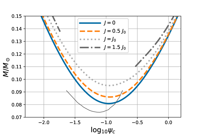
Figure 1: Critical curves of sustained nuclear reactions. Mass at which the condition $L_{n}/L_{s}=1$ is satisfied is plotted as functions of degeneracy $\psi_{c}$ at the center. On each curve, the angular momentum of the models is kept constant. For a model with $J=1.5J_{0}$, the bottom part of the curve is terminated at the mass-shedding limit, thus the curve is split into two branches. The gray solid curve is a plot of data taken from Fig.2 of Forbes & Loeb (2019) which assumes the opacity is one-tenth of that of electron scattering.

For each value of angular momentum, a model star located above the curve has a nuclear luminosity larger than the surface luminosity. The star may adjust itself to have higher $\psi_{c}$ while keeping its total mass constant (moves horizontally in the diagram), as far as the evolution proceeds with its mass conserved. Finally, it may sit on one of the critical curves with the same angular momentum. For slowly rotating stars with angular momentum $J\leq J_{0}=8.85\times 10^{48}({\rm erg}~{}{\rm s})$ the curve is continuous and has a minimum. The minimum corresponds to the smallest mass of the main sequence star, below which sustainable hydrogen burning does not take place.

As we increase the angular momentum, the critical curve is shifted upward and the minimum mass of the main sequence increases. When the total angular momentum is larger than $J_{0}$ the critical curve is split into two disjoint segments. This is because the lost portion of the curve corresponds to the model with mass-shedding at the equator and cannot be realized as hydrostatic equilibrium. The leftmost point on the branch with larger $\psi_{c}$ and the rightmost point on the branch with smaller $\psi_{c}$ are the mass-shedding limit models.

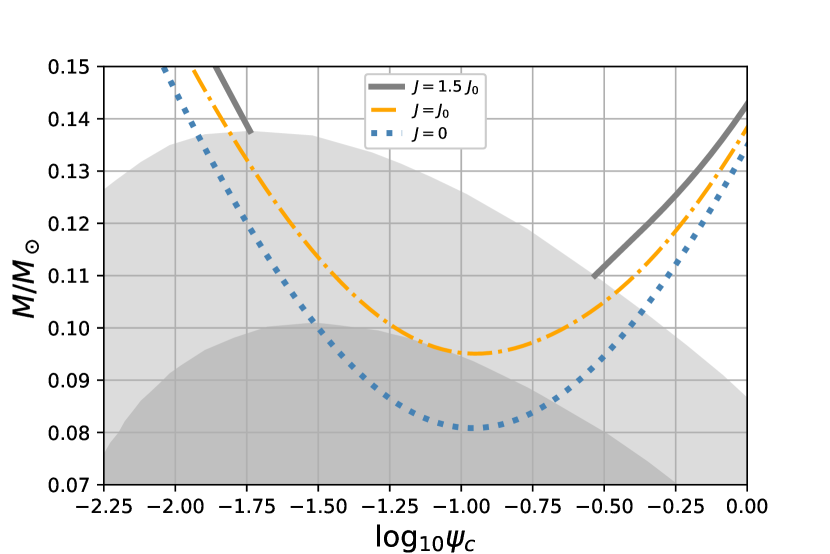
Figure 2: Parameter region of mass-shedding limit for fixed angular momentum value and the critical curves. The dash-dotted line is the critical curve for $J=J_{0}$. The dark-shaded region is the parameter region for mass-shedding models for $J=J_{0}$. The light-shaded region is the one for $J=1.5~{}J_{0}$.

In Fig.2 we show how the critical curves are split into two branches by the corresponding parameter region of mass-shedding. The parameter region of the mass-shedding limit (shaded) expands to a larger mass as angular momentum increases. For sufficiently small angular momentum ($J<J_{0}$) the critical curve is above this region. The critical curve becomes tangential to the boundary of the mass-shedding region when $J=J_{0}$. For larger angular momentum the critical curve is broken up by the mass-shedding region.

Fig.3 shows the contour of $L_{n}/L_{s}$ ratio for the fixed angular momentum $J=1.5~{}J_{0}$. The mass-shedding region in the parameter space splits the contour lines for $L_{n}/L_{s}\lesssim 10^{2}$. The parameter region of a successful hydrogen burning ($L_{n}/L_{s}=1$) is bounded by the mass-shedding region, therefore the minimum mass for the hydrogen burning is not determined as an extremum of the critical curve, but as the lighter model of the mass-shedding limit with $L_{n}/L_{s}=1$. It is therefore expected that a cooling evolution of an originally rapidly-rotating brown dwarf would be affected by the mass-shedding limit (see Sec.3.2).

Figure 3: Contour of $L_{n}/L_{s}$ value for $J=1.5~{}J_{0}$ stars. In the hatched region no equilibrium star exists with the fixed value of $J$ due to mass-shedding

In Fig.4, the minimum mass of the critical curve $L_{n}/L_{s}=1$ is plotted as a function of the angular momentum. A model below this curve does not become a main sequence star as far as the angular momentum is conserved. We see the mass-shedding limit starts affecting the minimum mass at $J=J_{0}$, where the curve has an inflection point. For $J\geq J_{0}$, the mass is limited by the mass-shedding limit. The dotted line is the mass of the branch with the stronger degeneracy, which is higher than the one with the weaker degeneracy. Thus the minimum mass corresponds to the model with the weaker degeneracy and the mass-shedding limit.

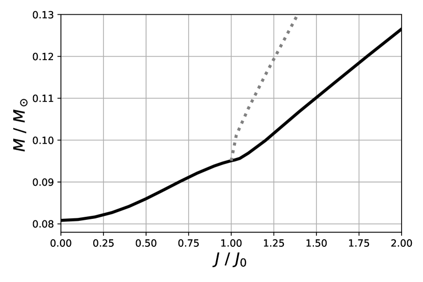
Figure 4: Minimum mass of the critical curve for given angular momentum (solid). The dotted line is the minimum mass of the critical curve branch with the stronger degeneracy (e.g., the left branch of $J=1.5J_{0}$ in Fig.1). This branch appears when $J>J_{0}$.

3.2 Simplified evolutionary paths of very low-mass stars and brown dwarfs

Spin-down of very low-mass objects is suggested by the comparison of rotational periods of stars in stellar clusters with different ages (see, e.g., Scholz & Eislöffel 2004, 2005). The origin of the spin-down mechanism is still debated since the classical spin-down mechanism of solar-type stars as magnetic breaking or winds may not be so effective in fully-convecting objects (Bouvier et al., 2014). Since the angular momentum loss is not well-understood at present, we here consider two simplified mechano-thermal evolution models of very low-mass objects assuming two extreme cases of angular momentum evolutions.

3.2.1 Efficient spin-down models

The first model assumes some external mechanism of spin-down to be sufficiently effective in the course of the cooling paths. This mechanism could be either magnetic braking, magnetic stellar wind, or interaction with a circumstellar disc. We simply parametrize angular momentum loss by introducing a constant spin-down timescale $\tau_{\rm sd}$. The angular momentum evolution is written as

$$\frac{dJ}{dt}=-\frac{J}{\tau_{\rm sd}}.$$ (28)

The cooling of a star is approximated by

$$\frac{d\psi_{c}}{dt}=-\frac{\psi_{c}}{\tau_{\rm cool}}.$$ (29)

The cooling timescale $\tau_{\rm cool}$ is computed by

$$\tau_{\rm cool}\equiv\frac{U}{L_{s}},$$ (30)

where $U$ is the internal energy of the model. Thus it is a function of $\psi_{c}$, $M$, and $J$. The process takes place in Kelvin-Helmholtz (K-H) timescale or spin-down timescale, which is anyway much longer than the hydrodynamic timescale. The mass loss by winds may be neglected compared with the angular momentum loss. We couple and solve Eq.(28) and (29) assuming total mass is conserved. The surface luminosity $L_{s}$ is computed at each time step. Here we terminate the computation when the stellar spin is approximately zero (axis ratio becomes 0.995) or it reaches mass-shedding limit.

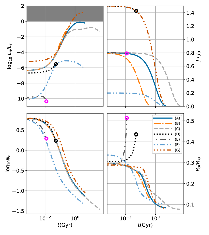
Figure 5: Spin-down evolutions of physical quantities. On each sequence the mass in units of $M_{\odot}$ is fixed while the angular momentum is lost with a constant timescale $\tau_{\rm sd}$ (see Eq.(28)) in units of Gyr. The initial angular momentum $J_{\rm ini}$ in units of $J_{0}$ is specified for each curve. The parameter set of the curves is the following. (A):$(M,J_{\rm ini},\tau_{\rm sd})=(0.08,0.8,1)$ ; (B):$(0.08,0.8,0.1)$; (C):$(0.08,0.8,10)$; (D):$(0.08,1.5,1)$; (E):$(0.04,0.8,1)$; (F):$(0.04,0.2,1)$; (G):$(0.1,1.5,1)$. The top left panel shows the luminosity ratio $\log_{10}(L_{n}/L_{s})$. The dark-hatched region marks the domain in which an object becomes a low-mass main sequence star. The top right is the angular momentum plot. The bottom left is the degeneracy parameter $\log_{10}\psi_{c}$. The bottom right is the equatorial radius in units of $R_{\odot}$. The open circles at the edge of sequences mark the occurrence of mass-shedding. Otherwise, a sequence terminates at a zero rotation model.

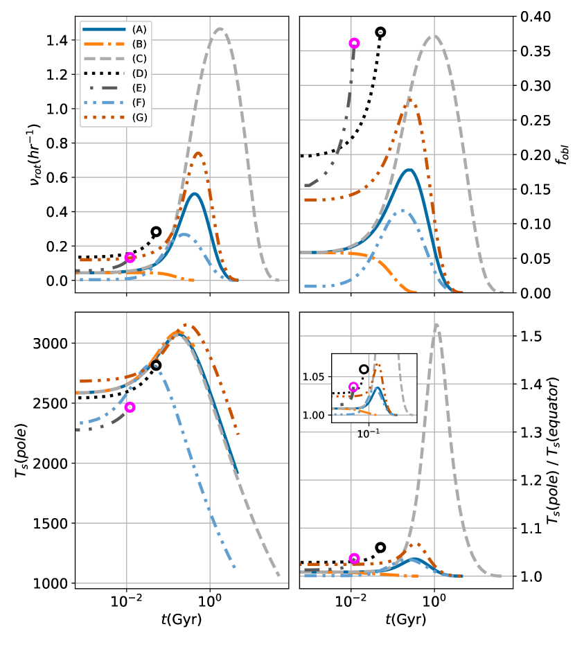
Figure 6: Evolution of additional physical variables for the same models as in Fig.5. The top left panel shows the rotational frequency $\nu_{\rm rot}$ in units of ${\rm hour}^{-1}$. The top right is the oblateness. The bottom left is the photospheric temperature $T_{s}$ at the pole. The bottom right is the ratio of the polar photospheric temperature to the equatorial one.

In Fig.5 and 6 spin-down evolutions of objects that conserve masses are exhibited. These figures share the same labels (A)-(G) for the models. On each sequence mass $M$ in units of $M_{\odot}$ is fixed. The sequences are additionally parameterized by the initial angular momentum $J_{\rm ini}$ in units of $J_{0}$ and the angular momentum loss rate $\tau_{\rm sd}$ in units of Gyr. The computation starts at $\log_{10}\psi_{c}=0.8$. The models (D) and (E) are initially rotating so rapidly that they eventually reach the mass-shedding limits which are marked by the open circles. The top-left panel of Fig.5 shows the evolution of the logarithmic luminosity ratio. The shaded area corresponds to the stable p-p chain reaction where an object turns into a main sequence star. For the low mass models with $M\leq 0.08$ it is always negative and the models never become main sequence stars. For more massive cases with $0.1M_{\odot}$, they reach the nuclear burning limit within 1Gyr time for $J_{\rm ini}=1.5J_{0}$.

As is seen in the bottom-left panel of Fig.5, the degeneracy monotonically decreases as an object radiates and contract. Comparing (A)-(D) and (E)-(F) we see the degeneracy evolution is mainly determined by the mass, with a very weak dependence on the initial angular momentum or the spin-down time. It should be noted that the model (G) reaches the nuclear burning limit before 1Gyr, after which the degeneracy for these models would cease to decrease. Our current model, however, does not follow this transition of an object to a very low-mass main sequence star.

The equatorial radius of an object may decrease monotonically except for the cases that reach the mass-shedding limit. (bottom-right in Fig.5). The radius evolution does not depend strongly on the mass, on the initial angular momentum, nor on the spin-down time.

In the top-left panel of Fig.6 we show the evolution of rotational frequency in units of ${\rm hour}^{-1}$. Rotational frequency changes non-monotonically while the angular momentum decreases monotonically. This is because the moment of inertia changes as the structure of the object evolves. Especially when the spin-down time is large, the star contracts while its angular momentum loss is small and it leads to a larger increase in the rotational frequency (compare (C) with (A) and (B)).

In the top-right panel of Fig.6 the oblateness $f_{\rm obl}$ is plotted. The oblateness of low mass objects may be potentially inferred through observation of polarized light (Barnes & Fortney, 2003; Sengupta & Marley, 2010). For the small $\tau_{\rm sd}$ model ($\tau_{\rm sd}=0.1$ Gyrs), the oblateness monotonically drops down to zero because of the rapid loss of angular momentum. It is noticed that the oblateness is not a monotonic function of time for a case with the larger value of $\tau_{\rm sd}$. The star initially becomes closer to a sphere but its oblateness increases and it diminishes again. The non-monotonic evolution of $f_{\rm obl}$ may be understood as follows. We remark that the oblateness scales as $\Omega^{2}$, where $\Omega$ is the rotational angular frequency, since the stellar deformation is induced by the centrifugal force. Then we write the total angular momentum $J$ as a function of the stellar radius $R_{s}$ and $f_{\rm obl}$ as $J=\alpha MR_{s}f_{\rm obl}$. The stellar mass $M$ is fixed in the evolution and $\alpha$ is a constant factor. Then the time derivative of $J$ gives

$$\frac{1}{J}\frac{dJ}{dt}=\frac{1}{R_{s}}\frac{dR_{s}}{dt}+\frac{1}{f_{\rm obl}}\frac{df_{\rm obl}}{dt},$$ (31)

or

$$\frac{1}{f_{\rm obl}}\frac{df_{\rm obl}}{dt}=-\tau_{\rm sd}^{-1}-\frac{1}{R_{s}}\frac{dR_{s}}{dt},$$ (32)

since we have $-\tau_{\rm sd}^{-1}$ as a negative constant (see Eq.(28)). When $R_{s}$ is decreasing in time (i.e., $dR_{s}/dt<0$), the sign of the left-hand side is determined by the time derivative of $R_{s}$. We first focus on (A) in Fig.5 whose spin-down timescale is 1Gyr. The decline of $R_{s}$ becomes steeper around $t\sim 0.25$Gyr. Then the $-d\log R_{s}/dt$ term becomes large enough to let $f_{\rm obl}$ increases. After that $f_{\rm obl}$ decreases again as the decline of $R_{s}$ later slows down. The model (C) has $\tau_{\rm sd}=10$Gyr. For this model, the first term on the left-hand side of Eq.(32) is smaller than that in (E). As a result, the duration of increasing $f_{\rm obl}$ is longer. The model (B) has $\tau_{\rm sd}=0.1$Gyr. This model spins down so quickly that the term of $-d\log R_{s}/dt$ has little effect on $f_{\rm obl}$ evolution. Then $f_{\rm obl}$ decreases monotonically.

The bottom-left panel is the effective temperature at the poles. The surface temperature slightly increases at first, then decreases because the cooling starts to dominate the sum of the nuclear energy generation and the liberation of gravitational binding energy. The temperature shows little dependence on $\tau_{\rm sd}$ or on the initial angular momentum.

As is shown in the bottom-right panel of Fig.6, the difference between the polar and the equatorial temperature may reach as much as 60% for the long spin-down time of $10$Gyr, but it is lower than 10% for the shorter timescale.

3.2.2 Decretion models

In another limiting case, the spin-down due to magnetic breaking or stellar wind may be neglected. Then the star may spin up by contracting while radiating away its energy, with the angular momentum being conserved. When the star hits its mass-shedding limit, it sheds part of its mass at the surface, which would form a disc/ring around the equator of the star. This is similar to the so-called ’decretion disc’ observed in Be stars (Lee et al., 1991; Okazaki, 2001). The decretion takes place in the K-H timescale which is much longer than the hydrodynamic timescale. Thus the star sheds its mass while maintaining hydrostatic equilibrium. Here we introduce a simple model of this decretion process. When a star is rotating at the mass-shedding limit, the gas element at the equatorial surface is orbiting the star at the Keplerian frequency. Then no pressure gradient is necessary for the element to stay there, and the element moves as if it were a test particle in the stellar gravitational field. Once the star cools and contracts, the element is left as it is, since forces acting on it do not change. As far as the stellar radius continues decreasing, the gas element orbiting with local Keplerian velocity forms a ring. The evolution of the system is driven by the cooling of the object and its timescale is that of K-H contraction. Strictly speaking, the gravitational potential of the whole system may change gradually as the stellar matter is re-distributed to disc.

We assume a spherical $N=1.5$ polytrope as a model of a uniformly rotating star neglecting rotational deformation. From the numerical solution of Lane-Emden equation for $N=1.5$, we find the mass $M_{r}$ contained inside the radius $r$ and the moment of inertia $I_{r}$ inside the cylindrical section of radius $r$ scales as $I_{r}\sim M_{r}^{\lambda}$ with $\lambda\sim 2.5$, for the matter close to the stellar surface. Suppose a uniformly rotating star with angular frequency $\Omega$ has the mass $M_{\star}$, the radius $R_{\star}$, the moment of inertia $I_{\star}$, and the angular momentum $J_{\star}$. When the star reaches the mass-shedding limit, it loses a small fraction of the outer part whose radial coordinate is larger than $r~{}(<R_{\star})$ for some value of $r$. Through this decretion process, the amount of angular momentum lost is $\Delta J=(I_{\star}-I_{r})\Omega$, which is simply advected outward with the decreted mass. Then we have

$$\frac{\Delta J}{J_{\star}}=1-\frac{I_{r}}{I_{\star}}.$$ (33)

Since we have a scaling of $I_{r}\sim M_{r}^{\lambda}$.

$$\frac{\Delta J}{J_{\star}}=1-\left(\frac{M_{r}}{M_{\star}}\right)^{\lambda}=1-\left(1-\frac{\Delta M}{M_{\star}}\right)^{\lambda},$$ (34)

where $\Delta M$ is the mass decreted. Then for $|\Delta M|/M_{\star}\ll 1$, we have

$$\frac{\Delta J}{J_{\star}}=\lambda\frac{\Delta M}{M_{\star}}.$$ (35)

Eq.(35) determines the mechano-thermal evolution of a star during the period of mass decretion. When the mass decretion starts, the star loses its mass and angular momentum. In the $\log_{10}\psi_{c}-M$ plane, the star then follows a path whose mass and angular momentum is determined by Eq.(35) and which is at the same time sitting on the mass-shedding contour with $J=J_{\star}-\Delta J$. This decretion process lasts as far as the star stays on a mass-shedding contour for the angular momentum it currently has. The sequence terminates either if it is not on the mass-shedding curve or if the radius of the star increases. Once the decretion ceases, the star resumes normal K-H contraction by preserving its mass and angular momentum.

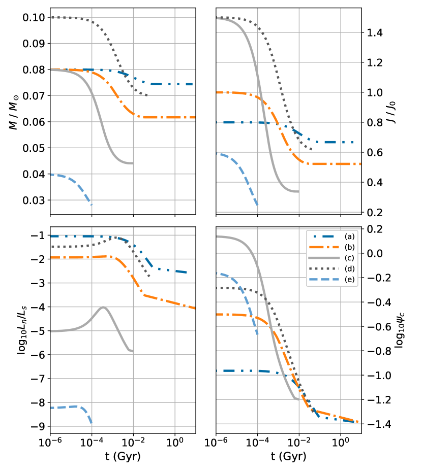
Figure 7: Evolutionary sequences of stars in the decretion processes. The parameter set for each curve is the following; (a):$(M(t=0),J(t=0))=(0.08,0.8)$; (b):$(0.08,1.0)$; (c):$(0.08,1.5)$; (d):$(0.1,1.5)$; (e):$(0.04,0.6)$. The top left panel shows the mass in units of $M_{\odot}$. The top right is the angular momentum in units of $J_{0}$. The bottom left is the luminosity ratio $\log_{10}(L_{n}/L_{s})$. The bottom right is the degeneracy parameter.

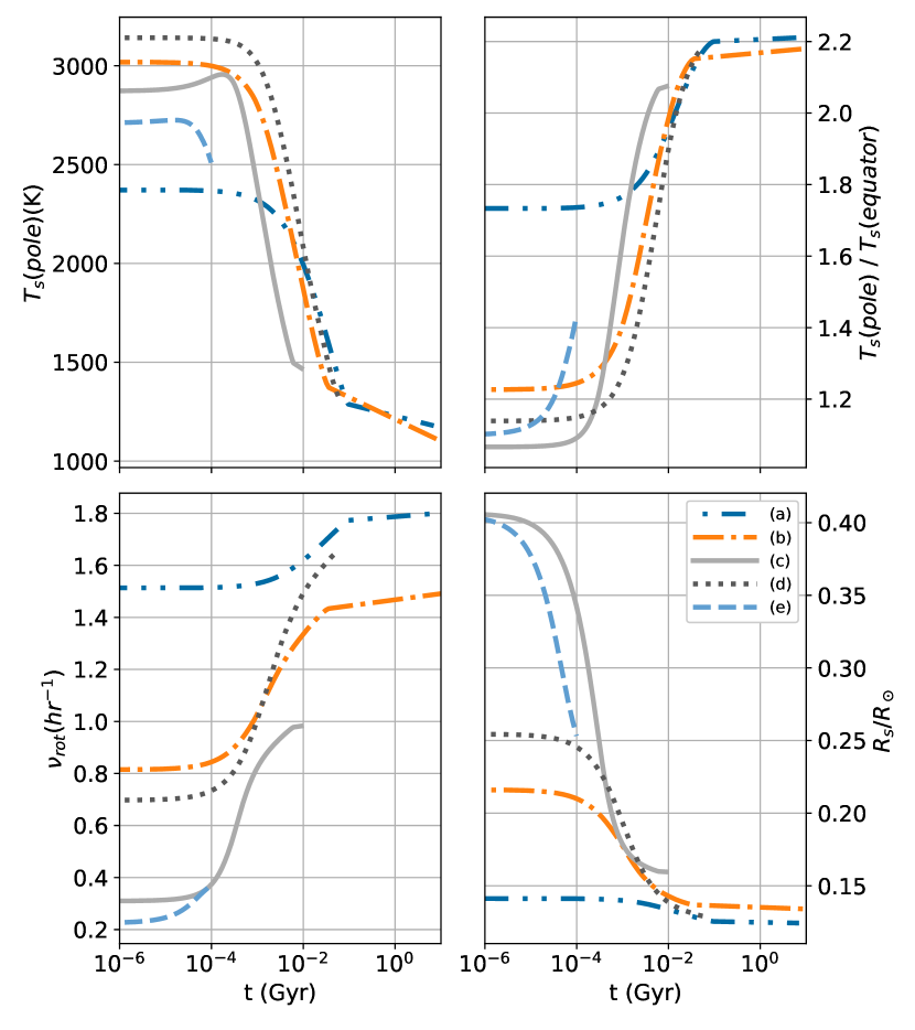
Figure 8: Evolution of additional physical quantities for the same models as in Fig.7. The top left is the photospheric temperature at the pole. In the top right is the ratio of polar to equatorial photospheric temperature. The bottom left is the rotational frequency in units of ${\rm hour}^{-1}$. The bottom right is the equatorial radius in units of $R_{\odot}$.

In Fig.7 and 8 evolutions of variables with mass-shedding sequences are shown. The origin of time is the initiation of the decretion process by mass-shedding. Each curve terminates at the end of the mass decretion process. These models are parametrized by their initial mass $M(t=0)$ and initial angular momentum $J(t=0)$.

From the top left and right panels in Fig.7 we see a significant fraction of the mass and angular momentum of an original object lost during the whole decretion process. Comparing the cases with $M(t=0)=0.08M_{\odot}$ with different initial angular momentum, we see that the larger the initial angular momentum, the stronger the decretion effect is. This is because the model with the larger angular momentum has the larger radius (see the bottom-right panel of Fig.8) and the larger moment of inertia, which is inferred from the top-right panel of Fig.7 and the bottom-left panel of Fig.8. This means the star with the larger $J(t=0)$ has a larger fraction of mass and angular momentum in the outer part of it, which are lost from the star during the decretion process. It means that for the models with the fixed initial mass, the mass and the angular momentum lost in the decretion process is larger when the star initially has a larger angular momentum.

As is seen in the bottom-right panel of 7 and the top panels of 8, the evolution of the degeneracy and the surface temperature at the later stage do not depend strongly on the mass nor on the initial angular momentum.

From the top panels of Fig.8, we see the surface temperature evolution does not strongly depend on the initial parameters.

A seemingly counter-intuitive trait of the rotational frequency is that it is lower for a higher initial angular momentum case, when the models with the same initial mass are compared. As is seen in the bottom-right panel of Fig.8, a star with a larger initial angular momentum has a larger initial radius. This is because the centrifugal force makes the star expand perpendicular to the rotational axis. The moment of inertia becomes larger for the higher initial angular momentum case and a model spins more slowly even if it has a larger angular momentum.

Finally, we may speculate on an outcome of the evolution of the substellar objects through the decretion process. The result of the decretion process may be a massive decretion disc surrounding a brown dwarf. If the disc survives long enough to accumulate a substantial fraction of the mass of the original dwarf, it may become gravitationally unstable and fragments into smaller bodies. The fragmentation may lead to the formation of a binary of brown dwarfs or a planetary system around a brown dwarf.

4 Summary and conclusion

We present numerical models of rotating very low-mass stars and brown dwarfs up to their mass-shedding limits. Rotation may strongly affect the occurrence of sustainable hydrogen burning in these objects by the introduction of centrifugal force to the hydrostatic balance as well as by the appearance of mass-shedding limit for rapidly rotating cases. Our model takes into account the non-perturbative effect of rotation on equilibrium figures of very low-mass objects. We obtain the critical curves of sustainable hydrogen burning in the degeneracy-mass plane, on which nuclear reaction rate equals the surface luminosity. As is expected, the critical curve for the higher value of angular momentum shift upward, thus the minimum mass for the stable hydrogen burning goes up as the angular momentum increases. There is a limiting value of angular momentum, $J_{0}=8.85\times 10^{48}$(erg s) beyond which the critical curve is no longer continuous in the parameter plane. For $J>J_{0}$, we find the minimum mass for hydrogen burning is constrained by the appearance of the mass-shedding limit.

We also use our models to study mechano-thermal evolutions of substellar objects that experience the Kelvin-Helmholtz contraction. Two extreme cases of conservative and non-conservative evolution of mass and angular momentum are studied. For the case of angular momentum loss by some external mechanism such as stellar wind or magnetic braking, the degeneracy parameter and the surface temperature do not strongly depend on the parameters except the total mass, while the stellar rotation frequency and the oblateness depends on the spin-down timescale. The rotational frequency and the oblateness do not evolve monotonically. The models having large initial angular momentum evolve toward the mass-shedding limit.

For the case with no external braking mechanism, a rotating model would follow first a path of Kelvin-Helmholtz contraction with mass and angular momentum being conserved. As it contracts, it may encounter its mass-shedding limit. If it reaches the mass-shedding limit before it satisfies a critical condition for sustained nuclear burning ($L_{n}/L_{s}=1$), the star starts its mass-decretion evolution by losing its excess angular momentum and mass to the surrounding disc/ring. We follow the mass-decretion process from the onset of mass-shedding limit. For given initial mass the decretion process takes place rapidly when the initial angular momentum is larger, which leads to the larger loss of mass and angular momentum. It is also remarkable that the rotational frequency monotonically increases though the angular momentum is lost by the decretion.

The end product of this decretion process may be a small brown dwarf and a debris disc. Or more interestingly, if the disc is gravitationally unstable, a binary system of brown dwarfs or a brown dwarf with a planetary system may form.

Data Availability

The data underlying this article will be shared upon reasonable request to the corresponding author.

Appendix A Gravity darkening of rotating very low mass objects

From von Zeipel’s theorem (von Zeipel, 1924) the effective surface temperature of a star is a function of surface gravity. Thus in a uniformly rotating star the surface temperature decreases as we go away from the rotational axis. The original theorem states that the temperature $T$ and the surface gravitational acceleration $g_{\rm eff}$ which includes the centrifugal contribution are related as

$$T\propto g_{\rm eff}^{\beta},$$ (36)

where $\beta=0.25$.

Figure 9: Gravity darkening of our rotating dwarf models. Surface temperature in Kelvin is plotted against the local acceleration of effective gravity $\tilde{g}_{\rm eff}$ which is normalized by $4\mathrm{\pi}G\rho_{c}R_{\rm eq}$, where $\rho_{c}$ is the central density and $R_{\rm eq}$ is the equatorial radius. On each curve, the polar point corresponds to the upper right while the equatorial point is at the lower left. The top panel is for a slowly rotating model (axis ratio is 0.96) with $\psi_{c}=0.139$ and $M=0.022M_{\odot}$. The second panel is for a rapidly rotating model (axis ratio is 0.68) with the same $\psi_{c}$ but $M=0.025M_{\odot}$. The third panel is for a rapidly rotating model with $\psi_{c}=0.788$ and $M=0.082M_{\odot}$ while the bottom panel is for a rapidly rotating model with $\psi_{c}=0.0185$ and $M=0.073M_{\odot}$. $\beta$ in each panel is the best-fit power-law index of von Zeipel-like dependence of gravity darkening.

Although the theorem applies only for barotropic stars where pressure depends solely on density, it is extended to the convective case by Lucy (1967). For this case, $T\propto g_{\rm eff}^{0.08}$. By introducing the Roche model and comparing it with their two-dimensional numerical models of rapidly rotating stars, Espinosa Lara & Rieutord (2011) show that the gravity darkening is well-represented by a power law neither by von Zeipel’s nor Lucy’s. Their effective power $\beta$ changes from $\beta\sim 0.25$ in non-rotating stars to $\beta\lesssim 0.14$ for the most rapidly rotating stars.

We see the gravity darkening in our rotating models. In Fig. 9 The surface temperature is plotted as a function of local effective gravity $g_{\rm eff}$. We see good power-law fittings of $T$ as a function of $g_{\rm eff}$, though the power index $\beta$ depends on the mass, the rotation, and the degeneracy of the model. For the models with relatively large degeneracy at the center (the first and second panel in Fig.9, $\beta\sim 0.12-0.14$ for both slowly and rapidly rotating cases. This suggests that the dependence of $\beta$ on the axis ratio or the oblateness is rather weak. Comparing the third and fourth panels, $\beta$ depends strongly on the degeneracy parameter. It should be noted the fitting quality by the power law becomes lower for rapidly rotating cases as is pointed out by Espinosa Lara & Rieutord (2011).

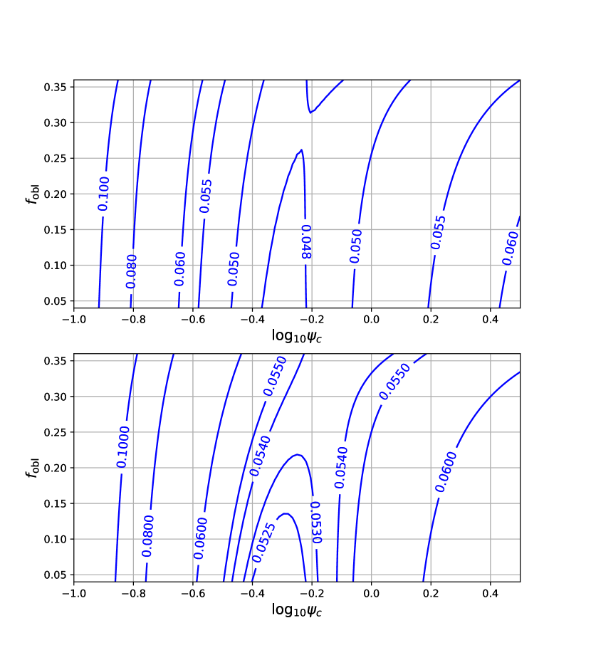
Figure 10: Contour of the power-law index $\beta$ of the gravity darkening law ($T_{\rm eff}\propto g_{\rm eff}^{\beta}$) in the $\log_{10}\psi_{c}$ - $f_{\rm obl}$ plane. The top panel is for $M=0.08M_{\odot}$, while the bottom one is for $M=0.04M_{\odot}$.

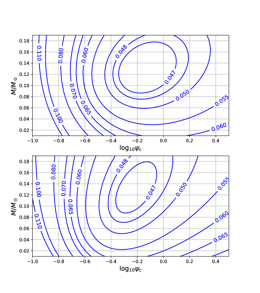
Figure 11: Contour of the power-law index $\beta$ for the fixed oblateness $f_{\rm obl}$, The top panel is for $f_{\rm obl}=0.37$ while the bottom one is for $f_{\rm obl}=0.02$.

$\beta$ is in general a function of degeneracy parameter $\psi_{c}$, mass $M$, and oblateness $f_{\rm obl}$. In Fig.10 the contour of $\beta$ in the $\log_{10}\psi_{c}$ - $f_{\rm obl}$ plane are given for $M=0.08M_{\odot}$ (top), and $M=0.04M_{\odot}$ (bottom).

In Fig.11 the contour in the $\log_{10}\psi_{c}$-$M$ plane are given for $f_{\rm obl}=0.37$ case (top), which are nearly mass-shedding limit, and for $f_{\rm obl}=0.02$ case (bottom), which are slowly rotating.

Appendix B Fitting formulae of numerical models

The curves in Sec.3 are drawn by using fitting formulae of numerical models. The fitting formulae are defined as functions of $\psi_{c}$, $M/M_{\odot}$, and ax, the axis ratio. $\psi_{c}$ measures how strong the degeneracy of a star is, or how strong the thermal effect is. $M$ measures the amount of mass and the strength of gravity. ${\rm ax}$ measures how fast the star is spinning. It should be noted that ${\rm ax}$ scales approximately as $\Omega^{2}$. All the fitting formulae below reproduce the parameter values computed numerically within the relative error of 10%.

Introducing $x=\log_{10}\psi_{c}$, $y=M/M_{\odot}$, $z=\sqrt{1-{\rm ax}}$ we fit the angular momentum of the star as,

$$\begin{split}J/10^{49}({\rm erg~{}s})&=\left[j_{0}+j_{1}x+j_{2}y+j_{3}x^{2}+j_{4}xy+j_{5}y^{2}\right]z\\ &\left[1+(j_{6}+j_{7}x+j_{8}y+j_{9}x^{2}+j_{10}xy+j_{11}y^{2})z\right]^{-1}\end{split}$$ (37)

$$\begin{split}&\mbox{{\rm where} {\rm fitted} {\rm parameters} {\rm are}}\\ &j_{0}=0.3360,j_{1}=0.7962,j_{2}=16.54,j_{3}=0.4079,j_{4}=6.228,\\ &j_{5}=51.74,j_{6}=0.2751,j_{7}=0.1035,\\ &j_{8}=-4.114,j_{9}=-0.08969,j_{10}=-1.621,\\ &j_{11}=10.48.\end{split}$$ (38)

$L_{n}/L_{s}$ is fitted by using $\zeta=1-{\rm ax}$ instead of $z$ as,

$$\begin{split}\log_{10}\left(\frac{L_{n}}{L_{s}}\right)&=\left[l_{0}(1+b_{01}\zeta+b_{02}\zeta^{2})+l_{1}(1+b_{11}\zeta+b_{12}\zeta^{2})x\right.\\ &+l_{2}(1+b_{21}\zeta+b_{22}\zeta^{2})y+l_{3}(1+b_{31}\zeta+b_{32}\zeta^{2})x^{2}\\ &\left.+l_{4}(1+b_{41}\zeta+b_{42}\zeta^{2})xy+l_{5}(1+b_{51}\zeta+b_{52}\zeta^{2})y^{2}\right]\\ &\left[1+l_{6}(1+b_{61}\zeta+b_{62}\zeta^{2})x+l_{7}(1+b_{71}\zeta+b_{72}\zeta^{2})y\right.\\ &+l_{8}(1+b_{81}\zeta+b_{82}\zeta^{2})x^{2}+l_{9}(1+b_{91}\zeta+b_{92}\zeta^{2})xy\\ &\left.+l_{10}(1+b_{101}\zeta+b_{102}\zeta^{2})y^{2}\right]^{-1}\end{split}$$ (39)

$$\begin{split}&\mbox{{\rm where} {\rm fitted} {\rm parameters} {\rm are}}\\ &l_{0}=-19.24,l_{1}=-19.90,l_{2}=89.97,l_{3}=-10.19,l_{4}=3.974,\\ &l_{5}=391.8,l_{6}=1.297,l_{7}=24.57,l_{8}=0.6119,\\ &l_{9}=4.902,l_{10}=27.84\\ &b_{01}=-1.306,b_{02}=4.715,b_{11}=-1.235,b_{12}=3.741,b_{21}=-1.699,\\ &b_{22}=6.480,b_{31}=-1.607,b_{32}=4.742,b_{41}=12.07,b_{42}=-39.57,\\ &b_{51}=-2.166,b_{52}=1.313,b_{61}=0.400,b_{62}=-2.504,b_{71}=-1.898,\\ &b_{72}=4.984,b_{81}=-0.07959,b_{82}=-1.657,b_{91}=-0.9873,b_{92}=1.038,\\ &b_{101}=-2.176,b_{102}=-1.816.\end{split}$$ (40)

Surface luminosity $L_{s}/L_{\odot}$ is fitted by

$$\begin{split}\log_{10}(L_{s}/L_{\odot})&=\left[q_{0}(1+c_{01}\zeta+c_{02}\zeta^{2})+q_{1}(1+c_{11}\zeta+c_{12}\zeta^{2})x\right.\\ &+q_{2}(1+c_{21}\zeta+c_{22}\zeta^{2})y+q_{3}(1+c_{31}\zeta+c_{32}\zeta^{2})x^{2}\\ &\left.+q_{4}(1+c_{41}\zeta+c_{42}\zeta^{2})xy+q_{5}(1+c_{51}\zeta+c_{52}\zeta^{2})y^{2}\right]\\ &\left[1+q_{6}(1+c_{61}\zeta+c_{62}\zeta^{2})x+q_{7}(1+c_{71}\zeta+c_{72}\zeta^{2})y\right.\\ &+q_{8}(1+c_{81}\zeta+c_{82}\zeta^{2})x^{2}+q_{9}(1+c_{91}\zeta+c_{92}\zeta^{2})xy\\ &\left.+q_{10}(1+c_{101}\zeta+c_{102}\zeta^{2})y^{2}\right]^{-1}\end{split}$$ (41)

$$\begin{split}&\mbox{{\rm where} {\rm fitted} {\rm parameters} {\rm are}}\\ &q_{0}=-2.244,q_{1}=-1.573,q_{2}=-17.40,q_{3}=--0.5792,q_{4}=-1.945,\\ &q_{5}=-9.714,q_{6}=0.9424,q_{7}=6.946,q_{8}=0.2706,\\ &q_{9}=2.597,q_{10}=2.012,\\ &c_{01}=0.1424,c_{02}=-0.4922,c_{11}=-0.06819,c_{12}=0.02784,\\ &c_{21}=-1.3035,c_{22}=2.486,c_{31}=1.487,c_{32}=-1.367,\\ &c_{41}=-1.977,c_{42}=0.9328,c_{51}=1.802,c_{52}=-2.004,\\ &c_{61}=-0.3951,c_{62}=0.8406,c_{71}=-0.9667,c_{72}=2.236,\\ &c_{81}=-0.2128,c_{82}=1.000,c_{91}=-0.9093,c_{92}=2.125,\\ &c_{101}=1.444,c_{102}=-1.342.\end{split}$$ (42)

Cooling timescale $\tau_{\rm cool}$ is fitted as

$$\begin{split}\log_{10}\left(\frac{\tau_{\rm cool}}{\rm 1Gyr}\right)&=\left[t_{0}(1+d_{01}\zeta+d_{02}\zeta^{2})+t_{1}(1+d_{11}\zeta+d_{12}\zeta^{2})x\right.\\ &+t_{2}(1+d_{21}\zeta+d_{22}\zeta^{2})y+t_{3}(1+d_{31}\zeta+d_{32}\zeta^{2})x^{2}\\ &\left.+t_{4}(1+d_{41}\zeta+d_{42}\zeta^{2})xy+t_{5}(1+d_{51}\zeta+d_{52}\zeta^{2})y^{2}\right]\\ &\left[1+t_{6}(1+d_{61}\zeta+d_{62}\zeta^{2})x+t_{7}(1+d_{71}\zeta+d_{72}\zeta^{2})y\right.\\ &+t_{8}(1+d_{81}\zeta+d_{82}\zeta^{2})x^{2}+t_{9}(1+d_{91}\zeta+d_{92}\zeta^{2})xy\\ &\left.+t_{10}(1+d_{101}\zeta+d_{102}\zeta^{2})y^{2}\right]^{-1}.\end{split}$$ (43)

$$\begin{split}&\mbox{{\rm where} {\rm fitted} {\rm parameters} {\rm are}}\\ &t_{0}=-2.945,t_{1}=-2.772,t_{2}=14.80,t_{3}=-0.4297,t_{4}=-0.3028,t_{5}=-3.997,\\ &t_{6}=0.8193,t_{7}=8.680,t_{8}=0.2258,t_{9}=2.969,t_{10}=-2.106\\ &d_{01}=-0.2074,d_{02}=0.6923,d_{11}=-2.353,d_{12}=4.824,d_{21}=2.790,\\ &d_{22}=-6.338,d_{31}=-12.00,d_{32}=22.26,d_{41}=-52.46,d_{42}=126.0,\\ &d_{51}=56.96,d_{52}=-121.9,d_{61}=-2.334,d_{62}=4.386,d_{71}=-2.896,\\ &d_{72}=5.579,d_{81}=-2.244,d_{82}=4.660,d_{91}=-4.350,\\ &d_{92}=8.542,d_{101}=20.32,d_{102}=-44.68\end{split}$$ (44)

References

- Allard et al. (2012) Allard F., Homeier D., Freytag B., 2012, Phil. Trans. R. Soc. London, Ser. A, 370, 2765
- Auddy et al. (2016) Auddy S., Basu S., Valluri S. R., 2016, Advances in Astronomy, 2016, 574327
- Baraffe et al. (1998) Baraffe I., Chabrier G., Allard F., Hauschildt P. H., 1998, A&A, 337, 403
- Baraffe et al. (2015) Baraffe I., Homeier D., Allard F., Chabrier G., 2015, A&A, 577, A42
- Barnes & Fortney (2003) Barnes J. W., Fortney J. J., 2003, ApJ, 588, 545
- Bouvier et al. (2014) Bouvier J., Matt S. P., Mohanty S., Scholz A., Stassun K. G., Zanni C., 2014, in Beuther H., Klessen R. S., Dullemond C. P., Henning T., eds, Protostars and Planets VI. p. 433 (arXiv:1309.7851), doi:10.2458/azu_uapress_9780816531240-ch019
- Burrows & Liebert (1993) Burrows A., Liebert J., 1993, Reviews of Modern Physics, 65, 301
- Burrows et al. (2001) Burrows A., Hubbard W. B., Lunine J. I., Liebert J., 2001, Reviews of Modern Physics, 73, 719
- Camenzind (2007) Camenzind M., 2007, Compact objects in astrophysics : white dwarfs, neutron stars, and black holes. Springer Berlin, Heidelberg, doi:10.1007/978-3-540-49912-1
- Chabrier & Baraffe (1997) Chabrier G., Baraffe I., 1997, A&A, 327, 1039
- Chabrier et al. (1992) Chabrier G., Saumon D., Hubbard W. B., Lunine J. I., 1992, ApJ, 391, 817
- Chowdhury et al. (2022) Chowdhury S., Banerjee P., Garain D., Sarkar T., 2022, ApJ, 929, 117
- Cox & Giuli (1968) Cox J. P., Giuli R. T., 1968, Principles of stellar structure. Gordon and Breach, New York
- Dantona & Mazzitelli (1985) Dantona F., Mazzitelli I., 1985, ApJ, 296, 502
- Espinosa Lara & Rieutord (2011) Espinosa Lara F., Rieutord M., 2011, A&A, 533, A43
- Forbes & Loeb (2019) Forbes J. C., Loeb A., 2019, ApJ, 871, 227
- Freedman et al. (2008) Freedman R. S., Marley M. S., Lodders K., 2008, ApJS, 174, 504
- Greiner et al. (2012) Greiner W., Rischke D., Neise L., Stöcker H., 2012, Thermodynamics and Statistical Mechanics. Classical Theoretical Physics, Springer, New York
- Hachisu (1986) Hachisu I., 1986, ApJS, 61, 479
- Hansen (1999) Hansen B. M. S., 1999, ApJ, 517, L39
- Hayashi & Nakano (1963) Hayashi C., Nakano T., 1963, Progress of Theoretical Physics, 30, 460
- Kumar (1962) Kumar S. S., 1962, AJ, 67, 579
- Lee et al. (1991) Lee U., Osaki Y., Saio H., 1991, MNRAS, 250, 432
- Lodders (2003) Lodders K., 2003, ApJ, 591, 1220
- Lucy (1967) Lucy L. B., 1967, Z. Astrophys., 65, 89
- Lynden-Bell & Tout (2001) Lynden-Bell D., Tout C. A., 2001, ApJ, 558, 1
- Majidi et al. (2022) Majidi D., Forbes J. C., Loeb A., 2022, ApJ, 932, 91
- Okazaki (2001) Okazaki A. T., 2001, PASJ, 53, 119
- Route & Wolszczan (2016) Route M., Wolszczan A., 2016, ApJ, 821, L21
- Salpeter (1992) Salpeter E. E., 1992, ApJ, 393, 258
- Scholz & Eislöffel (2004) Scholz A., Eislöffel J., 2004, A&A, 421, 259
- Scholz & Eislöffel (2005) Scholz A., Eislöffel J., 2005, A&A, 429, 1007
- Sengupta & Marley (2010) Sengupta S., Marley M. S., 2010, ApJ, 722, L142
- Shapiro & Teukolsky (1983) Shapiro S. L., Teukolsky S. A., 1983, Black holes, white dwarfs, and neutron stars : the physics of compact objects. A Wiley-Interscience Publication, New York
- Tannock et al. (2021) Tannock M. E., et al., 2021, AJ, 161, 224
- Timmes & Arnett (1999) Timmes F. X., Arnett D., 1999, ApJS, 125, 277
- Tsuji et al. (1996) Tsuji T., Ohnaka K., Aoki W., Nakajima T., 1996, A&A, 308, L29
- Williams et al. (2017) Williams P. K. G., Gizis J. E., Berger E., 2017, ApJ, 834, 117
- Yoshida (2019) Yoshida S., 2019, MNRAS, 486, 2982
- Yoshida (2021) Yoshida S., 2021, ApJ, 906, 29
- von Zeipel (1924) von Zeipel H., 1924, MNRAS, 84, 665