Experimental demonstration of input-output indefiniteness in a single quantum device

Abstract

At the fundamental level, the dynamics of quantum fields is invariant under the combination of time reversal, charge conjugation, and parity inversion. This symmetry implies that a broad class of effective quantum evolutions are bidirectional, meaning that the exchange of their inputs and outputs gives rise to valid quantum evolutions. Recently, it has been observed that quantum theory is theoretically compatible with a family of operations in which the roles of the inputs and outputs is indefinite. However, such operations have not been demonstrated in the laboratory so far. Here we experimentally demonstrate input-output indefiniteness in a photonic setup, demonstrating an advantage in a quantum game and showing incompatibility with a definite input-output direction by more than $69$ standard deviations. Our results establish input-output indefiniteness as a new resource for quantum information protocols, and enable the table-top simulation of hypothetical scenarios where the arrow of time could be in a quantum superposition.

I Introduction

A central result in quantum field theory is the CPT theorem (1), which states that the fundamental dynamics of quantum fields is invariant under inversion of time direction, charge, and parity. One consequence of this result is that, at the fundamental level, the roles of the inputs and outputs of physical processes are symmetric: while we normally treat systems at earlier times as the inputs and systems at later times as the outputs, the dynamical laws of quantum mechanics are indifferent to the direction of time, and one could consistently imagine an observer that describes nature in the backward mode, treating future systems as inputs and past systems as outputs.

The symmetry between the inputs and outputs in a quantum measurement process has been first observed by Aharonov, Bergmann, and Lebowicz (2), and the symmetric role of inputs and outputs of general quantum processes has attracted increasing attention in recent years (3; 4; 5; 6; 7; 8; 9; 10; 11; 12). Very recently, Ref.(13) proposed a mathematical framework for defining operations that probe quantum processes in coherent superposition of the forward and the backward mode, or in even more general forms of indefinite input-output direction. In principle, these operations could be used to formulate exotic scenarios where the arrow of time between two events is in a quantum superposition, as well as scenarios where a time-delocalized agent operates in a coherent superposition of the forward mode and the backward mode. The physical realizability of these scenarios, however, is still unclear. More pragmatically, quantum operations with indefinite input-output direction can be used to devise new protocols for quantum information processing. The ability to use quantum devices in an indefinite input-output direction has the potential to offer advantages over standard quantum protocols, in which quantum gates are used in a well definite input-output direction and arranged in a well defined order. Regarding the order, recent works have shown that indefiniteness offers a number of advantages, demonstrated both theoretically (14; 15; 16; 17; 18; 19; 20; 21) and experimentally (22; 23; 24; 25; 26; 27; 28; 29). Regarding the input-output direction, Ref. (13) showed an advantage in a game where the player has to establish a property of two unknown quantum devices. Another advantage, of thermodynamic nature, arises from a related work by Rubino and collaborators (30; 31). However, the potential of quantum operations with indefinite input-output direction is still largely unexplored, and up to date had not been experimentally demonstrated.

Here we report the first experimental realization of an operation with indefinite input-output direction, showing that a single photonic device implementing an unknown polarization rotation can be probed in a coherent quantum superposition of two alternative directions, giving rise to a coherent superposition of an unknown quantum evolution and its time-reversal. To enable this demonstration, we develop a general method for witnessing the use of a single quantum device in an indefinite input-output direction. We also demonstrate experimentally the advantage of indefinite direction in a quantum game, observing a reduction of the losing probability by more than 16 times compared to the best setup operating in a fixed direction. The experimental and theoretical results provided in this work establish input-output indefiniteness as a resource for quantum information protocols, and, at the same time, enable a table-top simulation of exotic scenarios where the arrow of time between two events could be indefinite.

II Results

Witnesses of input-output indefiniteness. We start by developing a method for experimentally certifying input-output indefiniteness. We adopt the general approach of witnesses of quantum resources (32), which includes notable examples such as entanglement witnesses (33) and, more closely related to our work, witnesses of indefinite causal order (34) and witnesses of causal connection (35). A witness for a given resource is an observable quantity that distinguishes between a resourceful setup and all resource-less setups. For example, an entanglement witness for a given entangled state is an observable that has negative expectation value for that state and non-negative expectation values for all unentangled states. In the following, we will construct witnesses that detect setups capable of using quantum devices in an indefinite input-output direction.

Let us start by summarizing the notion of indefinite direction. For many processes in nature, the role of the inputs and outputs can be exchanged. For example, consider the transmission of a quantum particle through a magnetic field. In this case, the roles of the entry and exit points are interchangeable, and both modes of transmission give rise to well-defined evolutions for the particle. Hereafter, a quantum device with exchangeable input and output ports will be called bidirectional.

A mathematical characterization of the bidirectional devices acting on a given quantum system was provided in (13): a device is bidirectional if the corresponding transformation of density matrices (both in the forward and in the backward direction) is a bistochastic quantum channel (36; 37), that is, a linear map $\mathcal{C}$ of the form $\mathcal{C}(\rho)=\sum_{i}C_{i}\rho C_{i}^{\dagger}$, where $\rho$ is the input density matrix, and $(C_{i})$ are square matrices satisfying the conditions $\sum_{i}C_{i}^{\dagger}C_{i}=\sum_{i}C_{i}C_{i}^{\dagger}=I$, $I$ being the identity matrix. If a bistochastic channel $\mathcal{C}$ describes the state change in the forward direction, then the state change in the backward direction is described by the bistochastic channel $\Theta(\mathcal{C})$ given by $\Theta(\mathcal{C}):\,\rho\mapsto\sum_{i}\theta(C_{i})\,\rho\,\theta(C_{i})^{\dagger}$, where the map $\Theta$ is called an input-output inversion, and $\theta(C_{i})$ is either unitarily equivalent to $C_{i}^{T}$, the transpose of $C_{i}$, or unitarily equivalent to $C_{i}^{\dagger}$, the adjoint of $C_{i}$. In the following, we will focus on the case where the input-output inversion is unitarily equivalent to the transpose.

A bidirectional quantum device can be used in two alternative input-output directions, giving rise either to the transformation $\mathcal{C}$ (forward process) or to the transformation $\Theta(\mathcal{C})$ (backward process). In addition, quantum mechanics allows for setups that coherently control the input-output direction, such as the setup shown in Figure 1. Mathematically, the possible setups that use a given bidirectional device are described by higher-order maps $\mathcal{S}$ that transform the input channel $\mathcal{C}$ into a new quantum channel $\mathcal{S}(\mathcal{C})$, describing the overall state transformation achieved by the setup. Such higher-order maps are known as quantum supermaps (38; 39; 15). In turn, a supermap $\mathcal{S}$ can be described by a positive operator $S$, acting on the tensor product Hilbert space $\mathcal{H}_{A_{\rm I}}\otimes\mathcal{H}_{A_{\rm O}}\otimes\mathcal{H}_{B_{\rm I}}\otimes\mathcal{H}_{B_{\rm O}}$, where $\mathcal{H}_{A_{\rm I}}$ ($\mathcal{H}_{A_{\rm O}}$) is the Hilbert space of the input (output) system of the initial channel $\mathcal{C}$, while $\mathcal{H}_{B_{\rm I}}$ ($\mathcal{H}_{B_{\rm O}}$) is the Hilbert space of the input (output) system of the final channel $\mathcal{S}(\mathcal{C})$ (see Methods for the details). Note that, since the original device $\mathcal{C}$ transforms a given quantum system into itself, the Hilbert spaces $\mathcal{H}_{A_{\rm I}}$ and $\mathcal{H}_{A_{\rm O}}$ have the same dimension, hereafter denoted by $d_{A}$.

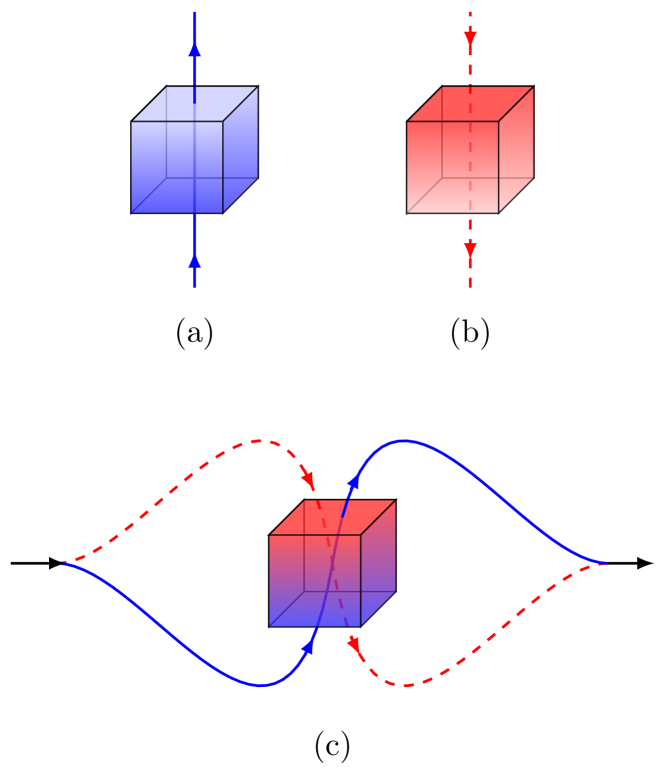
Figure 1: A bidirectional quantum device is a device that can be used both in the forward direction (a) or in the backward direction (b). More generally, bidirectional devices can be used in an indefinite input-output direction, resulting in a superposition of the forward process and the backward process (c).

A setup that uses the original device in the forward direction corresponds to a positive operator $S_{\rm fwd}$ satisfying the conditions $\operatorname{Tr}_{B_{\rm O}}[S_{\rm fwd}]=I_{A_{\rm O}}\otimes\operatorname{Tr}_{A_{\rm O}B_{\rm O}}[S_{\rm fwd}]/d_{A}$ and $\operatorname{Tr}_{A_{\rm O}A_{\rm I}B_{\rm O}}[S_{\rm fwd}]/d_{A}=I_{B_{\rm I}}$ (39). Similarly, a setup that uses the original device in the backward direction corresponds to a positive operator $S_{\rm bwd}$ satisfying the conditions $\operatorname{Tr}_{B_{\rm O}}[S_{\rm bwd}]=I_{A_{\rm I}}\otimes\operatorname{Tr}_{A_{\rm I}B_{\rm O}}[S_{\rm bwd}]/d_{A}$ and $\operatorname{Tr}_{A_{\rm O}A_{\rm I}B_{\rm O}}[S_{\rm bwd}]/d_{A}=I_{B_{\rm I}}$. More generally, a setup that uses the device in a randomly chosen direction will correspond to an operator of the form

$$S=p\,S_{\rm fwd}+(1-p)\,S_{\rm bwd}\,,$$ (1)

where $S_{\rm fwd}$ and $S_{\rm bwd}$ satisfy the above conditions, and $p$ is a probability. In the following, we will denote by $\mathsf{S}_{\rm definite}$ the convex set of all operators of the form (1). This set can be characterized by a finite number of semidefinite programming (SDP) constraints, similar to the constraints identified in Ref. (34) for the sets of setups compatible with definite causal order

Every setup corresponding to an operator $S$ outside $\mathsf{S}_{\rm definite}$ is incompatible with the existence of well-defined input-output direction. For an operator $S$ outside $\mathsf{S}_{\rm definite}$, we define a witness of input-output indefiniteness to be a multipartite operator $W$ acting on $\mathcal{H}_{A_{\rm I}}\otimes\mathcal{H}_{A_{\rm O}}\otimes\mathcal{H}_{B_{\rm I}}\otimes\mathcal{H}_{B_{\rm O}}$, such that

$$\operatorname{Tr}(WS)<0\,,$$ (2)

and

$$\operatorname{Tr}(WS^{\prime})\geq 0\,,\qquad\forall S^{\prime}\in\mathsf{S}_{\rm definite}\,.$$ (3)

A complete characterization of the possible witnesses of input-output indefiniteness is provided by the following Theorem, proved in Methods.

Theorem 1

An operator $W$ on $\mathcal{H}_{A_{\rm I}}\otimes\mathcal{H}_{A_{\rm O}}\otimes\mathcal{H}_{B_{\rm I}}\otimes\mathcal{H}_{B_{\rm O}}$ is a witness of input-output indefiniteness if and only if it can be decomposed as $W=W_{0}+W_{1}$, where $W_{0}$ and $W_{1}$ are operators satisfying the conditions

$$\operatorname{Tr}(W_{0}\,X)=0\,,\quad\forall X:\,\operatorname{Tr}_{A_{\rm I}A_{\rm O}B_{\rm O}}(X)=\frac{\operatorname{Tr}(X)}{d_{B_{\rm I}}}\cdot I_{B_{\rm I}}$$ (4)

and

$$W_{1}\geq W_{2}\,,\quad W_{1}\geq W_{3}\,,$$ (5)

for two operators $W_{2}$ and $W_{3}$ satisfying the conditions

$$\operatorname{Tr}(W_{2}\,Y)=0\,,\quad\forall Y:\,\operatorname{Tr}_{B_{\rm O}}(Y)=\operatorname{Tr}_{A_{\rm O}B_{\rm O}}(Y)\otimes\frac{I_{A_{\rm O}}}{d_{A}}$$

and

$$\operatorname{Tr}(W_{3}\,Z)=0\,,\quad\forall Z:\,\operatorname{Tr}_{B_{\rm O}}(Z)=\operatorname{Tr}_{A_{\rm I}B_{\rm O}}(Z)\otimes\frac{I_{A_{\rm I}}}{d_{A}}\,,$$

respectively.

In the following, the set of all witnesses of input-output indefiniteness will be denoted by $\mathsf{W}_{\rm in/out}$.

Every operator $W$ in Theorem 1 corresponds to an experimental scheme for detecting input-output indefiniteness in the laboratory. One approach to estimate $\operatorname{Tr}[W\,S]$ experimentally is to probe the action of the setup $S$ on a suitable input channel $\mathcal{C}$, possibly involving reference systems $R_{\rm I}$ and $R_{\rm O}$, and then to probe the action of the output process $(\mathcal{S}\otimes I_{R_{\rm I}\,R_{\rm O}})(\mathcal{C})$ by letting it act on a suitable input state, and measuring a suitable observable on the output. Here, $\mathcal{I}_{R_{\rm I}R_{\rm O}}$ is the identity supermap acting on the reference systems, and the input channel $\mathcal{C}$ is required to be locally bidirectional, in the sense that exchanging the roles of the systems $A_{\rm I}$ and $A_{\rm O}$, while keeping systems $R_{\rm I}$ and $R_{\rm O}$ fixed, should still give a valid quantum channel.

The value of the witness $\operatorname{Tr}(W\,S)$ can also be estimated without use of reference systems, by probing the action of the setup on a set of input processes, states, and observables. In this case, the input processes need to be the stochastic evolutions associated with bidirectional measurement processes, as discussed in Methods. An explicit example of this approach will be shown in the following section.

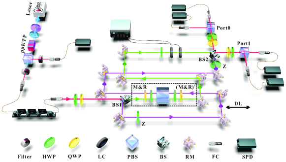
Figure 2: Experimental setup. A cw violet laser (2.5 mW power, working at 404 nm) pumps a type-II cut ppKTP crystal and generate a heralded single photon source after the idler photons trigger a single photon detector. Polarization of the photon serves as the target qubit and is initialized with a fiber polarizer controller, an HWP, and a QWP. Spatial modes of the photon serve as the control qubit and are introduced by BS1 to switch the time-bidirectional dynamics. Polarization dynamics is simulated with HWPs, QWP, and PBS, while measurements on spatial modes are realized with two LCs and BS2. A trombone-arm delay line and a piezoelectric transducer are used to set the path length and the relative phases of the interferometer. HWP, half wave plate; QWP, quarter wave plate; PBS, polarizing beam splitter; BS, beam splitter ($T/R=50/50$); RM, reflection mirror; LC, liquid crystal variable retarder; FC, fiber coupler; SPD, single photon detector; DL, trombone-arm delay line.

Experimental demonstration of input-output indefiniteness. We now use the method developed in the previous section to demonstrate input-output indefiniteness in a photonic setup. Our setup implements a theoretical primitive known as the quantum time flip (QTF) (13), in which a single quantum device is used in a coherent superposition of the forward and backward direction. The choice between the forward and backward direction is controlled by a quantum bit, and the control mechanism gives rise to an overall evolution of the form $\mathcal{F}(\mathcal{C}):\rho\mapsto\sum_{i}F_{i}\,\rho F_{i}^{\dagger}$, with

$$F_{i}=C_{i}\otimes|0\rangle\langle 0|+C_{i}^{T}\otimes|1\rangle\langle 1|\,,$$ (6)

where $|0\rangle$ and $|1\rangle$ are two orthogonal states of the control qubit, and $(C_{i})$ are the Kraus operators of the forward process $\mathcal{C}:\rho\mapsto\sum_{i}C_{i}\rho C_{i}^{\dagger}$ taking place inside the setup. If the control qubit is initialized in the state $|0\rangle$ ($|1\rangle$), then the overall process $\mathcal{F}(\mathcal{C})$ acts as the forward process $\mathcal{C}$ (backward process $\mathcal{C}^{T}$) on the target system. Instead, if the control qubit is initialized in a coherent superposition of $|0\rangle$ and $|1\rangle$, then the process $\mathcal{F}(\mathcal{C})$ implements a superposition of the processes $\mathcal{C}$ and $\mathcal{C}^{T}$ (3; 40; 41; 42; 42; 43; 44; 45; 46; 47; 48; 49; 50; 51; 52; 53; 54; 55; 27).

The setup of our experiment is shown in Fig. 2. A heralded single photon is generated by means of the process of spontaneous parametric down-conversion. The polarization qubit, serving as the target qubit in the quantum time flip, is initialized in an arbitrary fixed state, using a fiber polarizer controller, a half-wave plate (HWP) and a quarter-wave plate (QWP). The photon is sent to a 50/50 beamsplitter (BS1) to prepare the spatial qubit onto the state $|+\rangle=(|0\rangle+|1\rangle)/\sqrt{2}$, where $|0\rangle$ and $|1\rangle$ correspond to the two alternative paths shown green and carmine in Fig. 2. The input device for the quantum time flip is a bistochastic measure-and-reprepare process, implemented by an assemblage of HWPs, QWPs, a polarizing beam splitter (PBS), and single photon detectors, shown inside the dotted rectangle in Fig. 2. Measure-and-reprepare processes in the backward direction are realized by routing the photon through the same assemblage along a backward path sandwiched between two fixed Pauli gates $Z=|0\rangle\langle 0|-|1\rangle\langle 1|$. A coherent superposition of the forward and backward measure-and-reprepare processes is created by using the spatial degree of freedom of the same photon as a control qubit. Finally, two paths are coherently recombined on BS2, followed by a measurement on the polarization qubit. To maintain the coherent superposition, the measurement information on the target qubit is not read out until the information about the time direction of the evolution is erased at BS2.

To witness input-output indefiniteness, we adopt the witness that has maximum robustness with respect to noise. The theory of robustness for input-output indefiniteness is developed in Methods. There, we show that the optimal witness can be estimated by probing the setup on a set of stochastic quantum evolutions, corresponding to measurement processes that measure the polarization qubit in the eigenbasis of a Pauli gate and reprepare the output in a state in the eigenbasis of another Pauli gate. In our experiment, a basic set of projective measurements are realizaed by two HWPs, two QWPs and a PBS, and arbitrary other measurements are obtained by post-processing the experimental outcomes. The overall evolution induced by the setup is probed by initializing the path qubit in the maxially coherent state $|+\rangle$ and the polarization qubit in one of the states $|0\rangle$, $|1\rangle$, $|+\rangle$ and $\frac{1}{\sqrt{2}}(|0\rangle+i|1\rangle)$. Finally, the target qubit and control qubit are measured in the eigenbases of the three Pauli gates.

The experimental results are shown in Fig. 3, where we list a subset of the probabilities appearing in the decomposition of the optimal witness $W^{\rm opt}$ (See Appendix E for the remaining probabilities). The experimental probabilities of the terms are represented by blue rhombuses and the theoretical predictions are represented by red, cyan, yellow and green bars (corresponding to term in which the target qubit is prepared in $|0\rangle$, $|1\rangle$, $|+\rangle$ and $\frac{1}{\sqrt{2}}(|0\rangle+i|1\rangle)$ respectively). Some terms do not contribute to the decomposition of the witness so we do not test them and leave their probabilities blank. From these statistics, we calculate the experimental value of the robustness $r(S_{\rm QTF})$ to be $0.345\pm 0.005$, with the theoretical prediction being $0.4007$. These data demonstrate to more than 69 standard deviations that our setup is not compatible with a definite input-output direction. The mismatches of our experimental results and theoretical predictions are mainly caused by the phase drift of the Mach-Zenhder interferometer due to air turbulence and rotations of waveplates during the data collection.

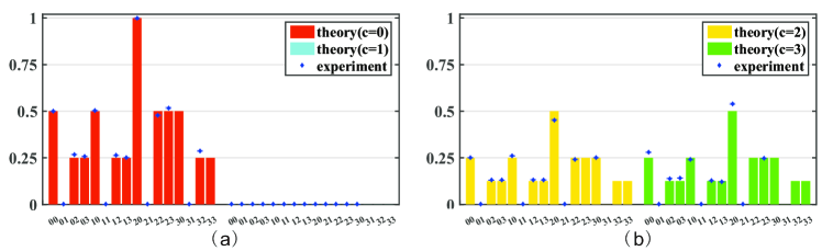
Figure 3: Probabilities of (a) the first 32 and (b) the next 32 terms in the decomposition of the witness $W^{\rm opt}$. The rhombuses represent the experimentally observed probabilities when choosing the initial state from an information complete set and the measure-and-reprepare operator is $|0\rangle\langle 0|$. The corresponding theoretical predictions shown in coloured bars (red, cyan, yellow, and green bars represent results when the initial state is $|0\rangle,|1\rangle,|+\rangle,\frac{1}{\sqrt{2}}(|0\rangle+i|1\rangle)$, corresponding to the labels $c=0$, $c=1$, $c=2$, $c=3$, respectively). The $x$ axis is labeled with the measurement outcomes of the control and target qubits, ‘23’ means that the qubits are projected onto $|+\rangle,\frac{1}{\sqrt{2}}(|0\rangle+i|1\rangle)$ for example. There are bars without corresponding experimental data because the coefficients of these terms are 0.

We note that, in order to detect input-output indefiniteness with the high statistical significance shown in our experiment, one needs to accurately control local operations on 5 qubits, using totally 794 settings. The complexity of the setup is still much less than the complexity of a full tomography of the setup, but the experiment is definitely demanding. One may therefore ask whether there one can find some weaker certification of input-output indefiniteness that can be achieved with less experimental effort. To this purpose, we provide an alternative witness of input-output indefiniteness which involves only 3 qubits and 48 settings. This is done by fixing the input of the target qubit to be $|0\rangle$ and by ignoring the final measurement on the target qubit (see Methods for more details). The theoretical value of the robustness of input-output indefiniteness decreases to $0.1716$, and the experimental value $0.140\pm 0.004$ (see Appendix E for the observed probabilities). Still, the violation of a definite input-output direction is detected by more than 35 standard deviations.

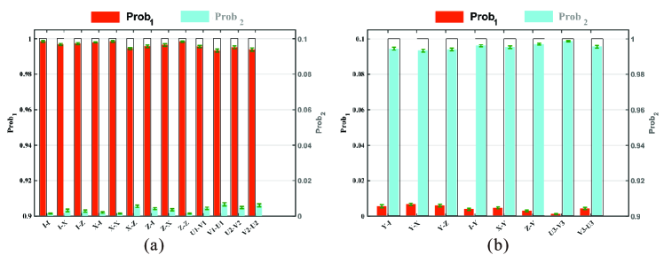
Figure 4: Results of unitary pairs selected from (a) $\mathsf{S}_{+}$ and (b) $\mathsf{S}_{-}$. The colored bars are the experimentally observed probabilities that detecting photons on port 0 (Prob₁, red bars, left vertical axis) and port 1 (Prob₂, cyan bars, right vertical axis), with the corresponding theoretical predictions shown in gray edges. The $x$ axis is labeled with the choice of gate pairs $(U,V)$ which are selected from either $\mathsf{S}_{+}$ or $\mathsf{S}_{-}$. The error bars of all the data are calculated from 100 simulations of Poisson statistics.

Experimental demonstration of advantage in a quantum game. Indefiniteness of the input-output direction can be leveraged as a resource in new quantum information tasks. A concrete example of this situation is a quantum game where a referee challenges a player to find out a hidden relation between two unknown quantum gates (13). The referee provides the player with two devices implementing unitary gates $U$ and $V$, respectively, promising that the two gates satisfy either the relation $UV^{T}=U^{T}V$ or the relation $UV^{T}=-U^{T}V$. The player’s task is to find out which of these two alternatives holds. Theoretical analysis showed that any player using the unknown gates in a well-defined direction will necessarily make mistakes at least 11% of the times. In contrast, a player that probes each gate with the quantum time flip can break this limit and reduce the error probability arbitrarily close to zero. Ideally, zero error probability can be achieved by using the quantum time flip to convert the given gates $U$ and $V$ into controlled gates $U\otimes|0\rangle\langle 0|+U^{T}\otimes|1\rangle\langle 1|$ and $V\otimes|0\rangle\langle 0|+V^{T}\otimes|1\rangle\langle 1|$, and then to connect them sequentially, obtaining the gate

$$UV^{T}\otimes|0\rangle\langle 0|+U^{T}V\otimes|1\rangle\langle 1|\,.$$ (7)

If the control qubit is initialized in the state $|+\rangle:=(|0\rangle+|1\rangle)/\sqrt{2}$, the relations $U^{T}V=UV^{T}$ and $U^{T}V=-UV^{T}$ give rise to perfectly distinguishable output states, which can be perfectly distinguished by measuring the control system at the output on the Fourier basis $\{|\pm\rangle:=(|0\rangle\pm|1\rangle)/\sqrt{2}\}$.

The experimental apparatus to implement the above strategy is shown in Appendix D. The spatial qubit is initialized in the state $|+\rangle$ by a 50/50 beamsplitter, while precise initialization of the polarization is not necessary here, since the winning strategy work equally well for every initial state of target system. Depending on the state of the spatial qubit, the target qubit undergoes two unitary gates $U$ and $V$ in different directions. Specifically, when the spatial qubit is $|0\rangle$, the system qubit undergoes $U^{T}V$ (green beam) and it undergoes $UV^{T}$ when the spatial qubit is $|1\rangle$ (carmine beam). The two paths are then coherently recombined on BS2, followed by a measurement on the polarization qubit. The photon exiting at port 0 corresponds to the outcome $|+\rangle$, and the photon exiting at port 1 corresponds to the outcome $|-\rangle$. To demonstrate the advantage of our setup in the quantum game, we tested a number of unitary gate pairs $\{(U_{i},V_{i})\}$ which satisfy either the condition $U_{i}V_{i}^{T}=U_{i}^{T}V_{i}$ (from set $\mathsf{S}_{+}$) or the condition $U_{i}V_{i}^{T}=-U_{i}^{T}V_{i}$ (from set $\mathsf{S}_{-}$). For example, we have $XZ^{T}=X^{T}Z$ and $XY^{T}=-X^{T}Y$, where $X$, $Y$ and $Z$ are Pauli gates (see Appendix D for details). The unitary gates can be implemented by rotating the wave plate angles appropriately (see Table I in Appendix D for details). We collected the photon events at the detectors to estimate the probabilities for the photons to exit each port. Our experiment results are shown in the bar diagram Fig. 4.

Theoretically, one can determine whether the tested gate pair is from set $\mathsf{S}_{+}$ or from set $\mathsf{S}_{-}$ with certainty as photons will all exit port 0 or port 1 for these two choices respectively. Our experimental results closely match this prediction, exhibiting an average success probability of $0.9960\pm 0.0018$. The maximal probability of error is approximate $0.68\%$, which is 16 times smaller than 11%, the lower bound of the probability of worst-case error of the strategies that use the gates in a fixed direction.

It is interesting to mention that the above quantum game can be regarded as a witness of input-output indefiniteness for bipartite setups (see Appendix B and C.

III Discussion

In this work we provided a general method for experimentally detecting the use of a single quantum device in an indefinite input-output direction. Equipped with this method, we provided the first experimental demonstration of input-output indefiniteness in a single quantum device. Our experimental setup allows one to perform not only unitary gates in a superposition of the forward and backward time direction, but also quantum measurements, enabling the measurement of arbitrary witnesses of input-output indefiniteness.

Our findings provide a complement to a recent series of experiments demonstrating indefinite gate order in table-top experiments (22; 23; 24; 25; 26; 27; 28; 29). In the future, indefinite input-output direction and indefinite order could be combined as building blocks for a new generation of setups that overcome the limitations of standard setups that use quantum devices in a fixed configuration, or in random mixture of alternative configurations.

On a more foundational side, the experimental investigation of processes with indefinite input-output can serve as a table-top simulation of exotic physics in which the arrow of time is a quantum variable, which could be in a coherent superposition of two opposite directions. These hypothetical phenomena fit into a broad framework developed by Hardy (6), who suggested that a full-fledged theory of quantum gravity would require a framework where the structure of spacetime is subject to indefiniteness. Furthermore, general processes with indefinite input-output direction can provide a theoretical model for studying time-delocalized agents with the ability to deterministically pre-select the state of certain systems and to deterministically post-select the state of other systems. While no physical model for indefinite time arrow or time-delocalized agents has been proposed up to date, the possibility to study the information-theoretic power of these scenarios, both theoretically and experimentally, provides an important instrument for understanding their potential operational implications.

IV Methods

Characterization of the witnesses. The characterization of the witnesses of input-output indefiniteness is conveniently expressed in terms of the Choi representation (56). The Choi representation of a linear $\mathcal{M}$, transforming operators on a Hilbert space $\mathcal{H}_{\rm in}$ into operators on a possibly different Hilbert space $\mathcal{H}_{\rm out}$ is given by

$$\operatorname{Choi}(\mathcal{M}):=(\mathcal{I}_{\rm in}\otimes\mathcal{M})(|I\rangle\!\rangle\langle\!\langle I|_{\rm in,in})\,,$$ (8)

where $|I\rangle\!\rangle_{\rm in,in}=\sum_{m}|m\rangle|m\rangle$ is the (unnormalized) maximally entangled quantum state on $\mathcal{H}_{\rm in}^{\otimes 2}$. In the following, we will denote by $L(\mathcal{H})$ the set of linear operators on a given Hilbert space $\mathcal{H}$.

For a quantum supermap $\mathcal{S}$, we can induce a map $\widehat{\mathcal{S}}$ on the Choi operators via the relation $\widehat{\mathcal{S}}$ : $\operatorname{Choi}(\mathcal{M})\mapsto\operatorname{Choi}(\mathcal{S}(\mathcal{M}))$, required to hold for every map $\mathcal{M}$.

Then we can define the Choi operator of $\mathcal{S}$ to be the Choi operator of the induced map $\widehat{S}$. With this notation, we are ready to provide our characterization of the set of all witnesses of input-output indefinitness.

Proof of Theorem 1. By definition, the collection $\mathsf{W}_{\rm in/out}$ is the dual cone of the collection $\mathsf{S}_{\rm definite}$, and $\mathsf{S}_{\rm definite}$ is the convex hull of the operators of forward setups and the operators of backward setups. Operators of forward setups can be extended to a convex cone of operators on $\mathcal{H}_{A_{\rm I}}\otimes\mathcal{H}_{A_{\rm O}}\otimes\mathcal{H}_{B_{\rm I}}\otimes\mathcal{H}_{B_{\rm O}}$ which is equal to $\mathcal{P}\cap\mathcal{L}_{V}\cap\mathcal{L}_{f}$, where $\mathcal{P}$ is the cone of positive operators, $\mathcal{L}_{V}$ is the subspace defined as

$$\mathcal{L}_{V}:=\left\{X\mid\operatorname{Tr}_{A_{\rm I}A_{\rm O}B_{\rm O}}(X)=\frac{\operatorname{Tr}(X)}{d_{B_{\rm I}}}\cdot I_{B_{\rm I}}\right\}$$ (9)

and $\mathcal{L}_{f}$ is the subspace defined as

$$\mathcal{L}_{f}:=\left\{Y\mid\operatorname{Tr}_{B_{\rm O}}(Y)=\operatorname{Tr}_{A_{\rm O}B_{\rm O}}(Y)\otimes\frac{I_{A_{\rm O}}}{d_{A}}\right\}\,.$$ (10)

Similarly, Operators of backward setups can be extended to a convex cone which is equal to $\mathcal{P}\cap\mathcal{L}_{V}\cap\mathcal{L}_{b}$, with $\mathcal{L}_{b}$ defined as

$$\mathcal{L}_{b}:=\left\{Z\mid\operatorname{Tr}_{B_{\rm I}}(Z)=\operatorname{Tr}_{A_{\rm O}B_{\rm I}}(Z)\otimes\frac{I_{A_{\rm O}}}{d_{A}}\right\}\,.$$ (11)

It follows that the conic hull of $\mathsf{S}_{\rm definite}$ is equal to

$$\begin{split}\operatorname{coni}(\mathsf{S}_{\rm definite})&=\operatorname{conv}[(\mathcal{P}\cap\mathcal{L}_{V}\cap\mathcal{L}_{f})\cup(\mathcal{P}\cap\mathcal{L}_{V}\cap\mathcal{L}_{b})]\\ &=\operatorname{conv}[(\mathcal{P}\cap\mathcal{L}_{f})\cup(\mathcal{P}\cap\mathcal{L}_{b})]\cap\mathcal{L}_{V}\,.\end{split}$$ (12)

The dual cone of $\mathsf{S}_{\rm definite}$ can be deduced using the duality properties of convex cones:

$$\begin{split}&\operatorname{coni}(\mathsf{S}_{\rm definite})^{*}\\ &=\operatorname{conv}\left[[(\mathcal{P}\cap\mathcal{L}_{f})^{*}\cap(\mathcal{P}\cap\mathcal{L}_{b})^{*}]\cup\mathcal{L}_{V}^{\perp}\right]\,\\ &=[(\mathcal{P}\cap\mathcal{L}_{f})^{*}\cap(\mathcal{P}\cap L_{b})^{*}]+\mathcal{L}_{V}^{\perp}\,,\\ &=[\operatorname{conv}(\mathcal{P}\cup\mathcal{L}_{f}^{\perp})\cap\operatorname{conv}(\mathcal{P}\cup\mathcal{L}_{b}^{\perp})]+\mathcal{L}_{V}^{\perp}\,,\\ &=[(\mathcal{P}+\mathcal{L}_{f}^{\perp})\cap(\mathcal{P}+\mathcal{L}_{b}^{\perp})]+\mathcal{L}_{V}^{\perp}\,,\end{split}$$ (13)

where $\perp$ denotes orthogonal complement and $+$ denotes Minkowski addition.

Now we can conclude from Eq. 13 that a Hermitian operator $W$ on $\mathcal{H}_{A_{\rm I}}\otimes\mathcal{H}_{A_{\rm O}}\otimes\mathcal{H}_{B_{\rm I}}\otimes\mathcal{H}_{B_{\rm O}}$ is a witness of input-output indefiniteness if and only if

$$W=W_{0}+W_{1}\,,$$ (14)

where $W_{1}\in\mathcal{L}_{V}^{\perp}$ and $W_{0}$ is a Hermitian operator such that

$$W_{0}\geq W_{2}\,,\quad W_{0}\geq W_{3}\,,$$ (15)

for some $W_{2}\in\mathcal{L}_{f}^{\perp}$ and $W_{3}\in\mathcal{L}_{b}^{\perp}$. $\blacksquare$

Measures of input-output indefiniteness. Witnesses can be used not only as a mean to detect resources, but also as a mean to define quantitative measures of that resource. This is done by assessing the robustness of a given resource to the addition of noise, as it was done, e.g. for the robustness of entanglement (57), robustness of causal indefiniteness (34), and robustness of causal connection (35). In our case, we consider the noise to be a general quantum supermap (13) that transform bistochastic channels to valid quantum channels. It corresponds to an operator $S_{\rm general}$ satisfying the conditions $\operatorname{Tr}_{A_{\rm O}A_{\rm I}B_{\rm O}}[S_{\rm general}]/d_{A}=I_{B_{\rm I}}$ and

$$\operatorname{Tr}_{B_{\rm O}}[S_{\rm general}]=\operatorname{Tr}_{B_{\rm O}A_{\rm O}}[S_{\rm general}]\otimes\frac{I_{A_{\rm O}}}{d_{A}}\\ +\operatorname{Tr}_{B_{\rm O}A_{\rm I}}[S_{\rm general}]\otimes\frac{I_{A_{\rm I}}}{d_{A}}\\ -\operatorname{Tr}_{B_{\rm O}A_{\rm O}A_{\rm I}}[S_{\rm general}]\otimes\frac{I_{A_{\rm O}}}{d_{A}}\otimes\frac{I_{A_{\rm I}}}{d_{A}}\,.$$ (16)

In the following we will denote the collection of operators of general supermaps by $\mathsf{S}$. We define the robustness of a setup $S$ with respect to a witness $W$ as

$$r(S\mid W):=\min_{T\in\mathsf{S}}\left\{\lambda\geq 0\mid\operatorname{Tr}\left(W\cdot\frac{S+\lambda T}{1+\lambda}\right)\geq 0\right\}\,,$$ (17)

which is equal to the amount of global worst-case noise the setup $S$ can tolerate such that it can still be detected by the witness $W$. The definition implies that the input-output indefiniteness of the setup $S$ can be detected by the witness $W$ only if the quantity $r(S\mid W)$ is larger than zero. Optimizing the quantity $r(S\mid W)$ over the witness $W$, we obtain the robustness of input-output indefiniteness of the setup $S$

$$r(S):=\max_{W\in\mathsf{W}_{\rm in/out}}r(S\mid W)\,.$$ (18)

Both Eq. 17 and Eq. 18 can be phrased as SDP problems and can be computed efficiently (see Appendix A). In particular, the quantity $r(S)$ is given by the following SDP:

maximize $$-\operatorname{Tr}(WS)$$ (19)

subject to $$W\in\mathsf{S}_{\rm definite}^{*}$$

$$\frac{I}{d_{A}d_{B_{\rm I}}}-W\in\mathsf{S}^{*}\,,$$

where $\mathsf{S}_{\rm definite}^{*}$ and $\mathsf{S}^{*}$ are the dual cones of $\mathsf{S}_{\rm definite}$ and $\mathsf{S}$, respectively. The last constraint of Eq. 19 can be interpreted as a normalization condition, noticing that for every setup $T$, the value $\operatorname{Tr}(WT)$ is no larger than 1, i.e.

$$\operatorname{Tr}(WT)\leq 1,\quad\forall T\in\mathsf{S}\,.$$ (20)

In addition, notice that the SDP problem in Eq. 19 has a similar form as the SDP problem in Eq. 38 of (34). So the input-output robustness also respects the axioms proposed in Ref. (34), i.e. it is a faithful ($r(S)$ is equal to zero if and only if $S$ is compatible with a well-defined input-output direction) and convex resource measure and can not be increased by composing the setup $S$ with local bistochatic channels.

Witnesses for the quantum time flip. We use the SDP in Eq. 19 to calculate the witness of input-output indefiniteness for QTF (denoted by $\mathcal{F}$). Suppose that the bidirectional devices are bistochastic channels from qubit $A_{\rm I}$ to qubit $A_{\rm O}$, $\mathcal{F}$ transform a bistochastic channel to another bistochastic channel whose input system is composed of a target input qubit $B_{it}$ and a control input qubit $B_{ic}$ and output system is composed of a target output qubit $B_{ot}$ and a control output qubit $B_{oc}$. The Choi operator of QTF, according to Ref. (13), is given by

$$\operatorname{Choi}(\mathcal{F})=|V\rangle\langle V|\,,$$ (21)

with

$$\begin{split}|V\rangle=&\,|I\rangle\!\rangle_{A_{\rm I}B_{it}}\otimes|I\rangle\!\rangle_{A_{\rm O}B_{ot}}\otimes|0\rangle_{B_{ic}}\otimes|0\rangle_{B_{oc}}\\ &+|I\rangle\!\rangle_{A_{\rm O}B_{it}}\otimes|I\rangle\!\rangle_{A_{\rm I}B_{ot}}\otimes|1\rangle_{B_{ic}}\otimes|1\rangle_{B_{oc}}\,.\end{split}$$ (22)

In the experiment, we set the initial state of the control qubit of QTF to be $|+\rangle=(|0\rangle+|1\rangle)/\sqrt{2}$, so theoretically Choi operator of the photonic circuit is

$$S_{\rm QTF}=|V^{+}\rangle\langle V^{+}|\,,$$ (23)

with

$$\begin{split}|V^{+}\rangle=&\,\frac{1}{\sqrt{2}}|I\rangle\!\rangle_{A_{\rm I}B_{it}}\otimes|I\rangle\!\rangle_{A_{\rm O}B_{ot}}\otimes|0\rangle_{B_{oc}}\\ &+\frac{1}{\sqrt{2}}|I\rangle\!\rangle_{A_{\rm O}B_{it}}\otimes|I\rangle\!\rangle_{A_{\rm I}B_{ot}}\otimes|1\rangle_{B_{oc}}\,.\end{split}$$ (24)

Solving the SDP problem in Eq. 19 with $S=S_{\rm QTF}$, we get the numerical matrix representation of the optimal witness $W^{\rm opt}$ and obtained the robustness value $0.4007$ of input-output indefiniteness.

To measure the witness $W^{\rm opt}$ in the experiment, we decompose it into a collection of linearly independent operations, including preparing the state of $B_{it}$, measuring the state of $A_{\rm I}$ and repreparing a state into $A_{\rm O}$, and measuring the state of $B_{ot}$ and $B_{oc}$. To be bidirectional, the measure-and-reprepare operations are required to be bistochastic instruments, i.e. the operators $\{M_{i}\}$ of such an instrument satisfy the condition that $\sum_{i}M_{i}$ is a bistochastic channel. In the case of QTF, we realized bistochastic instruments by measuring the system $A_{\rm I}$ in some basis $\{|v_{0}\rangle,|v_{1}\rangle\}$, then reprepare $|w_{0}\rangle$ ($|w_{1}\rangle$) from the basis $\{|w_{0}\rangle,|w_{1}\rangle\}$ if the outcome of measurement is 0 (1). Specifically, the decomposition is

$$W^{\rm opt}=\sum_{a,b,c,d,e}\alpha_{a,b,c,d,e}\Big{[}|a\rangle\langle a|_{B_{it}}\otimes|\overline{b}\rangle\langle\overline{b}|_{A_{\rm I}}\\ \otimes|c\rangle\langle c|_{A_{\rm O}}\otimes|\overline{d}\rangle\langle\overline{d}|_{B_{ot}}\otimes|\overline{e}\rangle\langle\overline{e}|_{B_{ot}}\Big{]}^{T}\,,$$ (25)

where $\alpha_{a,b,c,d,e}$ are real coefficients and the vectors $|a\rangle$, $|b\rangle$, $|c\rangle$, $|d\rangle$ and $|e\rangle$ are chosen from the following eigenstates of Pauli gates

$$|0\rangle,|1\rangle,\frac{|0\rangle+|1\rangle}{\sqrt{2}},\frac{|0\rangle+i|1\rangle}{\sqrt{2}}\,.$$ (26)

The number of terms that contribute to the decomposition of $W^{\rm opt}$ is 794. By Born’s rule, the probability of the event labeled by $(a,b,c,d,e)$ is

$$p(a,b,c,d,e)=\operatorname{Tr}\Big{[}\big{(}|a\rangle\langle a|_{B_{it}}\otimes|\overline{b}\rangle\langle\overline{b}|_{A_{\rm I}}\\ \otimes|c\rangle\langle c|_{A_{\rm O}}\otimes|\overline{d}\rangle\langle\overline{d}|_{B_{ot}}\otimes|\overline{e}\rangle\langle\overline{e}|_{B_{ot}}\big{)}^{T}S_{\rm QTF}\Big{]}\,.$$ (27)

In the experiment, we realized the relevant operations to estimate the probabilities $p(a,b,c,d,e)$. Then we obtained the experimental value $0.345\pm 0.005$ of the robustness of input-output indefiniteness according to the following equation:

$$\begin{split}r(S_{\rm QTF})&=-\operatorname{Tr}(W^{\rm opt}S_{\rm QTF})\\ &=-\sum_{a,b,c,d,e}p(a,b,c,d,e)\alpha_{a,b,c,d,e}\,.\end{split}$$ (28)

We also consider the witnesses of input-output indefiniteness which are less robust but can be operated by measuring only $A_{\rm I}$, $A_{\rm O}$, $B_{oc}$, fixing the state of $B_{it}$ to be $|0\rangle$ and tracing out $B_{ot}$. These witnesses can be computed by adding the following constraint to Eq. 19:

$$W=|0\rangle\langle 0|_{B_{it}}\otimes I_{B_{ot}}\otimes W^{\rm reduce}\,,$$ (29)

where $W^{\rm reduce}$ is a Hermitian matrix on $A_{\rm I}\otimes A_{\rm O}\otimes B_{oc}$. The maximal robustness of input-output indefiniteness under the above restriction is computed by the SDP in Eq. 19 (adding the constraint in Eq. 29) to be 0.1716. Let $W^{\prime}$ be the witness of input-output indefiniteness that achieves the maximal robustness under the constraint in Eq. 29. $W^{\prime}$ can then be decomposed and measured in the following way:

$$W^{\prime}=|0\rangle\langle 0|_{B_{it}}\otimes I_{B_{ot}}\otimes\\ \sum_{b,c,e}\beta_{b,c,e}\Big{[}|\overline{b}\rangle\langle\overline{b}|_{A_{\rm I}}\otimes|c\rangle\langle c|_{A_{\rm O}}\otimes|\overline{e}\rangle\langle\overline{e}|_{B_{ot}}\Big{]}^{T}\,,$$ (30)

where $\beta_{b,c,e}$ are real coefficients and the vectors $|b\rangle$, $|c\rangle$, and $|e\rangle$ are chosen from Eq. 26. The number of terms that contribute to the decomposition is 48 which is much less than the number of terms of the previous witness $W^{\rm opt}$. Again by Born’s rule and experimentally estimated probabilities $p(b,c,e)$, we got the experimental value $0.140\pm 0.004$ of the robustness of input-output indefiniteness by the following equation

$$r(S_{\rm QTF}\mid W^{\prime})=-\sum_{b,c,e}p(b,c,e)\beta_{b,c,e}\,.$$ (31)

V Data availability

The authors declare that the data supporting the findings of this study are available within the paper and in the supplementary information files.

VI Acknowledgments

The authors thank Ge Bai for stimulating discussion on the photonic realization of QTF. This work was supported by the National Key Research and Development Program of China (No. 2021YFE0113100, No. 2017YFA0304100), NSFC (No. 11734015, No. 11874345, No. 11821404, No. 11904357, No. 12174367, No. 12204458, and No. 17326616), the Hong Kong Research Grant Council through grants 17326616 (GC) and 17300918 (GC), and through the Senior Research Fellowship Scheme via SRFS2021-7S02 (GC), the Innovation Program for Quantum Science and Technology (No. 2021ZD0301200), the Fundamental Research Funds for the Central Universities, USTC Tang Scholarship, Science and Technological Fund of Anhui Province for Outstanding Youth (2008085J02), China Postdoctoral Science Foundation (2021M700138), China Postdoctoral for Innovative Talents (BX2021289). This work was partially carried out at the USTC Center

VII Author contributions

GC, BL, CL, and GG conceived the project and supervised the research. ZL developed the framework of witnesses of input-output indefiniteness and performed the numerical computations of the witnesses used in the experiments. BL and YG designed the experimental proposal. YG performed the experiment and analyzed the experimental data with the help of HT, XH, and YH. ZL, YG and GC wrote the manuscript. YG and ZL contributed equally.

VIII Competing interests

The authors declare no competing interests.

Appendix A Efficient computation of the robustness of input-output indefiniteness via SDP

A.1 Conic programming

Semidefinite programming is a special case of conic optimization which studies problems on minimizing a convex function over the intersection of an affine subspace and a convex cone. Theorem 4.2.1 of Ref. (58) provides the criterion of solving the conic programming problem efficiently with interior-point method. The conic programming problem is defined as

Definition 1

Let $E$ be a finite-dimensional vector space, $\mathcal{K}$ a closed convex pointed cone in $E$ with a nonempty interior, and $\mathcal{L}$ a linear subspace of $E$. Let also $b\in E$ and $c\in E$. The data $E$, $\mathcal{K}$, $\mathcal{L}$, $b$, and $c$ define a pair of conic problems

$$(P): \quad\textup{minimize}\ \langle c,x\rangle\quad\textup{subject to}\quad x\in\mathcal{K}\cap(\mathcal{L}+b),$$

$$(D): \quad\textup{minimize}\ \langle y,b\rangle\quad\textup{subject to}\quad y\in\mathcal{K}^{*}\cap(\mathcal{L}^{\perp}+c),$$

where $\mathcal{K}^{*}\subset E$ is the cone dual to $\mathcal{K}$, $\mathcal{L}^{\perp}\subset E$ is the orthogonal complement to $\mathcal{L}$, $\mathcal{L}+b\subset E$ and $\mathcal{L}^{\perp}+c\subset E$ are affine subspaces. (P) and (D) are called, respectively, the primal and dual problems associated with the above data.

Theorem 4.2.1 of Ref. (58) is presented in the following theorem.

Theorem 2

Let (P), (D) be a primal-dual pair of conic problems as defined above, and let the pair be such that

1. The set of primal solutions $\mathcal{K}\cap(\mathcal{L}+b)$ intersects $\operatorname{int}\mathcal{K}$;

2. The set of dual solutions $\mathcal{K}^{*}\cap(\mathcal{L}^{\perp}+c)$ intersects $\operatorname{int}\mathcal{K}^{*}$;

3. $\langle c,x\rangle$ is lower bounded for all $x\in\mathcal{K}\cap(\mathcal{L}+b)$.

Then both the primal and the dual problems are solvable, and the optimal solutions $x^{*}$ and $y^{*}$ satisfy the relation

$$\langle c,b\rangle=\langle c,x^{*}\rangle+\langle y^{*},b\rangle.$$ (32)

A.2 The SDP problems for the robustness of input-output indefiniteness

In analogy with the causal robustness from Ref. (34), we can formulate the robustness of input-output indefiniteness into SDP problems that can be solved efficiently. The quantity $r(S\mid W)$, which is the generalized robustness of a setup $S$ with respect to a witness $W$, can be formulated into the following SDP problems (simply letting the variable $\lambda$ be absorbed into the variable $T$ in Eq. 17 in the main text):

minimize $$\frac{\operatorname{Tr}(T)}{d_{B_{\rm I}}d_{A}}$$ (33)

subject to $$\operatorname{Tr}[W(S+T)]\geq 0$$

$$T\in\operatorname{coni}(\mathsf{S})\,.$$

The dual problem of the above problem is

maximize $$-y\operatorname{Tr}(WS)$$ (34)

$$\frac{I}{d_{B_{\rm I}}d_{A}}-yW\in\operatorname{coni}(\mathsf{S})^{*}$$

$$y\geq 0\,.$$

Here the notation $\operatorname{coni}$ denotes the conic hull. We will show that strong duality holds in the primal-dual pair 33 and 34, which means that the dual problem 34 also gives the robustness of input-output indefiniteness $r(S\mid W)$. It follows that the maximal robustness of input-output indefiniteness of $S$ is given by the following SDP problem (by letting the variable $y$ be absorbed by the variable $W$ in Eq. 34):

maximize $$-\operatorname{Tr}(WS)$$ (35)

$$W\in\operatorname{coni}(\mathsf{S}_{\rm definite})^{*}$$

$$\frac{I}{d_{B_{\rm I}}d_{A}}-W\in\operatorname{coni}(\mathsf{S})^{*}\,.$$

The problem 35 is exactly the SDP problem in Eq. 19 of the main text. Its dual problem is

minimize $$\frac{\operatorname{Tr}(T)}{d_{B_{\rm I}}d_{A}}$$ (36)

subject to $$S+T\in\operatorname{coni}(\mathsf{S}_{\rm definite})$$

$$T\in\operatorname{coni}(\mathsf{S})\,.$$

A.3 The SDP problems are efficiently solvable

In the following, we will use the the notation ${}_{X}\cdot$ which denotes the operation that traces out the subsystem $X$ and replacing it by the normalized identity operator, i.e.

$${}_{X}S=\operatorname{Tr}_{X}S\otimes\frac{I_{X}}{d_{X}}\,.$$ (37)

Here we show that the primal-dual SDP pairs (33, 34) and (36, 35) can be translated into the language of Definition 1 and satisfy the conditions of Theorem 2. We define the following data of a conic problem:

$$\begin{split}E&=(\mathcal{L}_{s}\cap\mathcal{L}_{V})\times(\mathcal{L}_{s}\cap\mathcal{L}_{V})\,,\\ \mathcal{L}&=\{(T,T)\mid T\in\mathcal{L}_{s}\cap\mathcal{L}_{V}\}\,,\\ b&=(S,0)\,,\\ c&=\left(0,\frac{I}{d_{B_{\rm I}}d_{A}}\right)\,,\end{split}$$ (38)

where $\mathcal{L}_{V}$, $\mathcal{L}_{f}$, $\mathcal{L}_{b}$ are the subspaces defined in the proof of Theorem 1 in the main text and $\mathcal{L}_{s}$ is defined as

$$\mathcal{L}_{s}:=\Big{\{}S\mid{}_{[B_{\rm O}]}S={}_{[B_{\rm O}A_{\rm O}]}S+{}_{[B_{\rm O}A_{\rm I}]}S-{}_{[B_{\rm O}A_{\rm O}A_{\rm I}]}S\Big{\}}\,.$$ (39)

For the pair (33, 34), we define

$$\mathcal{K}_{1}=\{T\in\operatorname{coni}(\mathsf{S})\mid\operatorname{Tr}(WT)\geq 0\}\times\operatorname{coni}(\mathsf{S})\,.$$ (40)

For the pair (36, 35), we define

$$\mathcal{K}_{2}=\operatorname{coni}(\mathsf{S}_{\rm definite})\times\operatorname{coni}(\mathsf{S})\,.$$ (41)

As mentioned in the main text, $\mathcal{L}_{f}\cap\mathcal{L}_{V}$ is the linear span of the operators of forward setups, $\mathcal{L}_{b}\cap\mathcal{L}_{V}$ is the linear span of the operators of backward setups, $\mathcal{L}_{s}\cap\mathcal{L}_{V}$ is the linear span of the operators of general supermaps on bistochastic channels.

The following lemma shows that a random mixture of the identity operator and an arbitrary operator from $\mathcal{L}_{s}\cap\mathcal{L}_{V}$ can be contained in the convex cone of $\mathsf{S}_{\rm definite}$.

Lemma 1

$I+S\in\operatorname{coni}(\mathsf{S}_{\rm definite})$ for operator $S\in\mathcal{L}_{s}\cap\mathcal{L}_{V}$ with norm $\|S\|_{2}\leq 1/2$, where $\|\cdot\|_{2}$ is the Hilbert–Schmidt norm.

Proof. This proof is similar to the proof of Lemma 7 of (34). Let $S$ be such an operator. $I+S$ can be decomposed into $S_{f}+S_{b}$ where

$$S_{f}=\frac{I}{2}+{}_{A_{\rm O}}S\,,\quad S_{b}=\frac{I}{2}+S-{}_{A_{\rm O}}S\,.$$ (42)

We can check that $S_{f}\in\mathcal{L}_{f}\cap\mathcal{L}_{V}$ and $S_{b}\in\mathcal{L}_{b}\cap\mathcal{L}_{V}$. Notice that ${}_{A_{\rm O}}S$ and $S-{}_{A_{\rm O}}S$ are orthogonal. By Pythagoras’ theorem, it holds that

$$\|{}_{A_{\rm O}}S\|_{2}^{2}+\|S-{}_{A_{\rm O}}S\|_{2}^{2}=\|S\|_{2}^{2}\,.$$ (43)

Therefore,

$$\max\{\|{}_{A_{\rm O}}S\|,\|S-{}_{A_{\rm O}}S\|\}\\ \leq\max\{\|{}_{A_{\rm O}}S\|_{2},\|S-{}_{A_{\rm O}}S\|_{2}\}\leq\|S\|_{2}\leq\frac{1}{2}\,,$$ (44)

where $\|\cdot\|$ is the standard operator norm (i.e. the maximal singular value). Therefore, both $S_{f}$ and $S_{b}$ are positive. So, $S_{f}\in\mathcal{P}\cap\mathcal{L}_{V}\cap\mathcal{L}_{f}$ and $S_{b}\in\mathcal{P}\cap\mathcal{L}_{V}\cap\mathcal{L}_{b}$. It follows that $I+S$ belongs to $\operatorname{coni}(\mathsf{S}_{\rm definite})$. $\blacksquare$

Now we check that the three conditions of Theorem 2 for the two pairs of SDP problems (33, 34) and (36, 35). Let $S$ be the Choi operator of a setup.

1. Since $\|S\|_{2}\leq\|S\|_{1}=\operatorname{Tr}(S)=d_{B_{\rm I}}d_{A}$, Lemma 1 implies that

   $$S+\lambda I\in\operatorname{coni}(\mathsf{S}_{\rm definite})\,,\quad\forall\lambda\geq 2d_{B_{\rm I}}d_{A}\,.$$ (45)

   So by choosing $\lambda_{0}>2d_{B_{\rm I}}d_{A}$, we have $(\lambda_{0}I,\lambda_{0}I)\in\mathcal{L}$ and

   $$b+(\lambda_{0}I,\lambda_{0}I)=(S+\lambda_{0}I,\lambda_{0}I)\in\operatorname{int}\mathcal{K}_{2}\,.$$ (46)

2. Let $W_{0}=\frac{I}{2d_{B_{\rm I}}d_{A}}$. We have $(W_{0},-W_{0})\in\mathcal{L}^{\perp}$ and

   $$(W_{0},-W_{0})+c=(W_{0},W_{0})\,.$$ (47)

   $(W_{0},W_{0})$ is an internal point of the dual cone of $\mathsf{S}\times\mathsf{S}$ because $\operatorname{Tr}(W_{0}T)=\operatorname{Tr}(W_{0}T^{\prime})=1/2>0$ for every $T,T^{\prime}\in\mathsf{S}$.

3. Both 33 and 36 are lower bounded by 0 because $T$ is a positive operator.

Due to the relation

$$\mathcal{K}_{2}\subseteq\mathcal{K}_{1}\subseteq\operatorname{coni}(\mathsf{S})\times\operatorname{coni}(\mathsf{S})\,,$$ (48)

we have

$$\operatorname{int}(\mathcal{K}_{2})\subseteq\operatorname{int}(\mathcal{K}_{1})\,,$$ (49)

and

$$\operatorname{int}((\operatorname{coni}(\mathsf{S})\times\operatorname{coni}(\mathsf{S}))^{*})\subseteq\operatorname{int}(\mathcal{K}_{1}^{*})\subseteq\operatorname{int}(\mathcal{K}_{2}^{*})\,.$$ (50)

It follows that the two pairs of SDP problems (33, 34) and (36, 35) satisfy the three conditions of Theorem 2 and thus can be solved efficiently.

Appendix B Choi representation of multipartite quantum supermaps on no-signaling bistochastic channels

B.1 Choi representation of bipartite quantum supermaps

In the following, we denote the set of quantum channels from system $A$ to system $B$ by ${\mathsf{Chan}}(A,B)$.

Theorem 3

A Hermitian operator $S$ is the Choi representation of a supermap from no-signaling bistochastic channels of type ${\mathsf{Chan}}(A_{\rm I}\otimes B_{\rm I},A_{\rm O}\otimes B_{\rm O})$ to quantum channels of type ${\mathsf{Chan}}(C_{\rm I},C_{\rm O})$ if

$$\operatorname{Tr}(S)=d_{C_{\rm I}}d_{A}d_{B}\,,$$ (51a)

$$S\geq 0\,,$$ (51b)

$${}_{[(1-C_{\rm I})A_{\rm I}A_{\rm O}B_{\rm I}B_{\rm O}C_{\rm O}]}S=0\,,$$ (51c)

$${}_{[(1-A_{\rm I})(1-A_{\rm O})B_{\rm I}B_{\rm O}C_{\rm O}]}S=0\,,$$ (51d)

$${}_{[(1-B_{\rm I})(1-B_{\rm O})A_{\rm I}A_{\rm O}C_{\rm O}]}S=0\,,$$ (51e)

$${}_{[(1-A_{\rm I})(1-A_{\rm O})(1-B_{\rm I})(1-B_{\rm O})C_{\rm O}]}S=0\,.$$ (51f)

Here we use the shorthand notation

$${}_{\left[\sum_{X}\alpha_{X}X\right]}S=\sum_{X}\alpha_{X}\cdot{}_{X}S\,.$$ (52)

Proof. A supermap is a CP map thus $S\geq 0$ (Eq. 51b). The requirement that $S$ transforms any bistochastic channel $\mathcal{N}_{1}\in{\mathsf{Chan}}(A_{\rm I},A_{\rm O})$ and bistochastic channel $\mathcal{N}_{2}\in{\mathsf{Chan}}(B_{\rm I},B_{\rm O})$ into a quantum channel in ${\mathsf{Chan}}(C_{\rm I},C_{\rm O})$ is equivalent to the condition

$$\operatorname{Tr}_{A_{\rm I}A_{\rm O}B_{\rm I}B_{\rm O}C_{\rm O}}[S(\operatorname{Choi}(\mathcal{N}_{1})\otimes\operatorname{Choi}(\mathcal{N}_{2})\otimes I_{C_{\rm I}C_{\rm O}})^{T}]\\ =I_{C_{\rm I}}\,.$$ (53)

According to the space of bistochastic channels (13), we can decompose the Choi operator of a bistochastic channel into operators, one of which is propositional to the identity and the others are tensor product of traceless operators on the input and output systems . Then the condition in Eq. 53 is equivalent to the following two conditions:

$$\operatorname{Tr}_{A_{\rm I}A_{\rm O}B_{\rm I}B_{\rm O}C_{\rm O}}[S]/(d_{A}d_{B})=I_{C_{\rm I}}\,,$$ (54)

which implies Eq. 51a and Eq. 51c; and

$$\operatorname{Tr}_{A_{\rm I}A_{\rm O}B_{\rm I}B_{\rm O}C_{\rm O}}[S(N_{1}\otimes N_{2}\otimes I_{C_{\rm I}C_{\rm O}})]=0\,,$$ (55)

for every pair of traceless operators $N_{1}$ and $N_{2}$. The linear space of operators on a Hilbert space has an orthogonal basis which contains the identity operator. After decomposing $S$ in the tensor product of such bases of $A_{\rm I}$, $A_{\rm O}$, $B_{\rm I}$, $B_{\rm O}$, $C_{\rm I}$, and $C_{\rm O}$, we can obtain the conditions in Eq. 51d, 51e and 51f. $\blacksquare$

The bipartite supermaps can exhibit both indefinite time direction and indefinite causal order (examples can be found in Ref. (13)). The extension of supermaps with definite time direction to multipartite cases is not trivial because of the existence of dynamic configuration of input-output directions (similar to the dynamic configuration of causal orders (59)). Here we present the conditions of the bipartite supermaps which use no-signaling bistochastic channels in a single fixed direction. $S$ is the Choi operator of a forward supermap (38; 39), if it satisfies the conditions in Eq. 51 and the following conditions which are stricter than Eq. 51d, 51e and 51f:

$${}_{[(1-A_{\rm O})B_{\rm I}B_{\rm O}C_{\rm O}]}S=0\,,$$ (56)

$${}_{[(1-B_{\rm O})A_{\rm I}A_{\rm O}C_{\rm O}]}S=0\,,$$ (57)

$${}_{[(1-A_{\rm O})(1-B_{\rm O})C_{\rm O}]}S=0\,.$$ (58)

Similarly, $S$ is the Choi operator of a backward supermap if it satisfies the conditions in Eq. 51 and additional conditions stricter than Eq. 51d, 51e, 51f:

$${}_{[(1-A_{\rm I})B_{\rm I}B_{\rm O}C_{\rm O}]}S=0\,,$$ (59)

$${}_{[(1-B_{\rm I})A_{\rm I}A_{\rm O}C_{\rm O}]}S=0\,,$$ (60)

$${}_{[(1-A_{\rm I})(1-B_{\rm I})C_{\rm O}]}S=0\,.$$ (61)

B.2 Extension to $N$-partite supermaps

The extension to $N$-partite supermaps is straight forward.

Theorem 4

A Hermitian operator $S$ is the Choi representation of a supermap from no-signaling bistochastic channels of type ${\mathsf{Chan}}(A_{1i}\otimes\cdots\otimes A_{Ni},A_{1o}\otimes\cdots\otimes A_{No})$ to quantum channels of type ${\mathsf{Chan}}(B_{\rm I},B_{\rm O})$ if

$$\operatorname{Tr}(S)=d_{B_{\rm I}}\prod_{k=1}^{N}d_{A_{k}}\,,$$ (62a)

$$S\geq 0\,,$$ (62b)

$${}_{[(1-B_{\rm I})A_{1i}\cdots A_{Ni}A_{1o}\cdots A_{No}B_{\rm O}]}S=0\,,$$ (62c)

and for all $2^{N}-1$ non-empty subsets $\mathcal{X}$ of $\{1,\cdots,N\}$,

$${}_{\prod_{x\in\mathcal{X}}(1-A_{xi})(1-A_{xo})\prod_{x\notin\mathcal{X}}A_{xi}A_{xo}B_{\rm O}}S=0\,.$$ (63)

Appendix C The (weak) witness of input-output indefiniteness induced by the quantum game

The quantum game introduced in the main text from Ref. (13) can be viewed as a (weak) witness of input-output indefiniteness. The strategies of the game can be described by bipartite supermaps which have two slots (corresponding to systems $A_{\rm I}\otimes A_{\rm O}$ and $B_{\rm I}\otimes B_{\rm O}$) and one qubit output $C_{\rm O}$. The strategy is carried out by placing the two gates $U$ and $V$ in the slots and then measuring the output qubit $C_{\rm O}$ in Fourier basis $\{|\pm\rangle\}$ which gives the outcome that $(U,V)$ belongs to

$$\mathsf{G}_{+}=\{(U,V)\mid UV^{T}=U^{T}V\}\,,$$ (64)

or

$$\mathsf{G}_{-}=\{(U,V)\mid UV^{T}=-U^{T}V\}\,.$$ (65)

Let $S$ be the Choi operator of the strategy. If the gates $(U,V)\in\mathsf{G}_{+}$, then the probability of winning is

$$\operatorname{Tr}((\operatorname{Choi}(U)\otimes\operatorname{Choi}(V)\otimes|+\rangle\langle+|)^{T}S)\,.$$ (66)

If the gates $(U,V)\in\mathsf{G}_{-}$, then the probability of winning is

$$\operatorname{Tr}((\operatorname{Choi}(U)\otimes\operatorname{Choi}(V)\otimes|-\rangle\langle-|)^{T}S)\,.$$ (67)

In the general case, suppose that $\mu(U,V)$ is a probability measure on $\mathsf{G}_{+}\cup\mathsf{G}_{-}$. We define the operators $M_{+}$ and $M_{-}$ to be

$$M_{\pm}:=\int_{\mathsf{G}_{\pm}}(\operatorname{Choi}(U)\otimes\operatorname{Choi}(V)\otimes|\pm\rangle\langle\pm|)^{T}{\rm d}\mu(U,V)\,.$$ (68)

Then the probability of winning is

$$p_{\rm succ}=\\ \int_{\mathsf{G}_{+}}\operatorname{Tr}((\operatorname{Choi}(U)\otimes\operatorname{Choi}(V)\otimes|+\rangle\langle+|)^{T}S)\cdot{\rm d}\mu(U,V)\\ +\int_{\mathsf{G}_{-}}\operatorname{Tr}((\operatorname{Choi}(U)\otimes\operatorname{Choi}(V)\otimes|-\rangle\langle-|)^{T}S)\cdot{\rm d}\mu(U,V)\\ =\operatorname{Tr}((M_{+}+M_{-})S)\,.$$ (69)

Ref. (13) shows that if the strategy $S$ uses the gates in a fixed direction, then the probability of winning is strictly smaller than 1. However, those who have access to QTF can win the game with unit probability. Let $p_{\max}$ ($p_{\max}<1$) denotes the maximal winning probability with strategies that uses the gates in a fixed direction. We can induce the following (weak) witness of input-output indefiniteness which detects the strategy with access to QTF:

$$W_{\rm game}=\frac{I}{d^{2}}-\frac{M_{+}+M_{-}}{p_{\max}}\,,$$ (70)

where $d$ is the dimension of the systems $A_{\rm I}$, $A_{\rm O}$, $B_{\rm I}$ and $B_{\rm O}$.

The witness $W_{\rm game}$ is a weak witness of input-output indefiniteness because there exist quantum strategies that use both gates in definite directions but can not be decomposed into those that use the gates in a single fixed direction. Such a quantum strategy does not has input-output indefiniteness yet wins the game with unit probability. The strategy is based on the quantum SWITCH supermap (15) which is a bipartite supermap with indefinite causal order. The two gates $U$ and $V$ are used in opposite directions. After placing them in the quantum SWITCH supermap with the control qubit set to the state $|+\rangle=(|0\rangle+|1\rangle)/\sqrt{2}$ and the target system set to half of the maximally entangled state, the output of the setup becomes

$$\frac{|UV^{T}+V^{T}U\rangle\!\rangle}{2\sqrt{d}}\otimes|+\rangle+\frac{|UV^{T}-V^{T}U\rangle\!\rangle}{2\sqrt{d}}\otimes|-\rangle.$$ (71)

Here we use the double-ket notation defined as

$$|M\rangle\!\rangle=\sum_{ij}\langle i|M|j\rangle\cdot|j\rangle\otimes|i\rangle\,.$$ (72)

Noticing that the vectors $|UV^{T}+V^{T}U\rangle\!\rangle$ and $|UV^{T}-V^{T}U\rangle\!\rangle$ are orthogonal if $(U,V)$ is in either $\mathsf{G}_{+}$ or $\mathsf{G}_{-}$, we can do a measurement to distinguish the vectors $|UV^{T}+V^{T}U\rangle\!\rangle$ and $|UV^{T}-V^{T}U\rangle\!\rangle$ and then measure the control qubit in Fourier basis $\{|\pm\rangle\}$. The above measurements are equivalent to the following measurement:

$$\{P\otimes|+\rangle\langle+|+(I-P)\otimes|-\rangle\langle-|,\\ (I-P)\otimes|+\rangle\langle+|+P\otimes|-\rangle\langle-|\}\,,$$ (73)

where $P$ is the projector onto the the subspace $\{|A\rangle\!\rangle\mid A=A^{T}\}$. The outcomes of the measurement perfectly correspond to the relations $(U,V)\in\mathsf{G}_{+}$ and $(U,V)\in\mathsf{G}_{-}$.

Appendix D Single photon source and unitary gates used in the game

We generated heralded single photon source via a SPDC process on a type-II cut ppKTP crystal. The crystal was pumped by focusing a 2.5 mW diode laser centered at 404 nm on it using a convex lens (focal length is 12.5 cm). Setting the polarization of the pump laser to be horizontal, we generated pairs of correlated photons centered at 808 nm in a polarization state $|H\rangle|V\rangle$, which were then separated by a PBS. The pump laser was blocked with long pass and narrow band pass filters. After this, the photon pairs were coupled into single-mode fibers, and the idler photon was used as a herald and the signal photon was sent to our experiment. The observed coincidence rate of the photon source was about 20000 pairs per second and was attenuated to 1850 pairs per second after the signal photon passing through the whole apparatus.

As discussed in the main text, to verify the information-theoretic advantage of indefiniteness of the input-output direction, we need to implement several unitary gate pairs $(U,V)$. The gate pairs satisfy either $UV^{T}=U^{T}V$ or $UV^{T}=-U^{T}V$. Specifically we consider the following two sets which were used in Ref. (13) to obtain a lower bound of probability of error in the strategies that use the gates in a single fixed direction:

$$\mathsf{S}_{+}= \{(I,I),(I,X),(I,Z),(X,I),(X,X),(X,Z),$$

$$(Z,I),(Z,X),(Z,Z),(U1,V1),(V1,U1),$$

$$(U2,V2),(V2,U2)\}\,,$$ (74)

$$\mathsf{S}_{-}= \{(Y,I),(Y,X),(Y,Z),(I,Y),(X,Y),(Z,Y),$$

$$(U3,V3),(V3,U3)\}\,,$$ (75)

where $I$ is identity gate and $X$, $Y$, $Z$ are Pauli gates. The unitary gates used in our experiment are listed in Table 1. As shown in Fig. 5, we implemented these gates using a combination of three waveplates (in a quarter-half-quarter configuration) and the angle settings are shown in Table 1.

Unitary gate	QWP1	HWP	QWP2
$I$	$0^{\circ}$	$0^{\circ}$	$0^{\circ}$
$X$	$0^{\circ}$	$45^{\circ}$	$0^{\circ}$
$Y$	$90^{\circ}$	$45^{\circ}$	$0^{\circ}$
$Z$	$90^{\circ}$	$0^{\circ}$	$0^{\circ}$
$U1=(X-Y)/\sqrt{2}$	$45^{\circ}$	$67.5^{\circ}$	$135^{\circ}$
$V1=(X+Y)/\sqrt{2}$	$135^{\circ}$	$67.5^{\circ}$	$45^{\circ}$
$U2=(Z-Y)/\sqrt{2}$	$0^{\circ}$	$22.5^{\circ}$	$90^{\circ}$
$V2=(Z+Y)/\sqrt{2}$	$90^{\circ}$	$22.5^{\circ}$	$0^{\circ}$
$U3=(I-iY)/\sqrt{2}$	$22.5^{\circ}$	$135^{\circ}$	$67.5^{\circ}$
$V3=(I+iY)/\sqrt{2}$	$67.5^{\circ}$	$135^{\circ}$	$22.5^{\circ}$

Table 1: The chosen unitary gates and corresponding setting angles of QWPs and HWPs for preparing these gates in our experiment.

Appendix E Supplementary figures

In this section, we present the probabilities of the remaining terms of the decomposition of the witness $W^{\rm opt}$ (Fig. 6-9) and the experimentally friendly witness $W^{\prime}$ (Fig. 10).

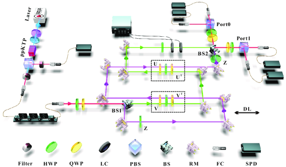
Figure 5: Experimental setup for the game in the main text. The core idea of this experiment is analogous to the one for the input-output indefiniteness witness. The only difference is the measure-and-reprepare process in the quantum time flip are replaced with the unitary gates $U$ and $V$. HWP, half wave plate; QWP, quarter wave plate; PBS, polarizing beam splitter; BS, beam splitter ($T/R=50/50$); RM, reflection mirror; LC, liquid crystal variable retarder; FC, fiber coupler; SPD, single photon detector; DL, trombonearm delay line.

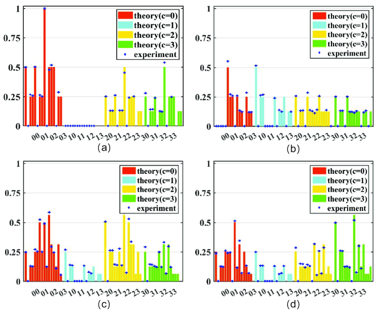
Figure 6: Probabilities in the the decomposition of the witness $W^{\rm opt}$ when the measure-and-reprepare maps are projection on $|0\rangle$ and reset on (a) $|0\rangle$, (b) $|1\rangle$, (c) $|+\rangle$, and (d) $\frac{1}{\sqrt{2}}(|0\rangle+i|1\rangle)$. The dots represents the experimentally observed probabilities and the corresponding theoretical predictions shown in coloured bars (red, cyan, yellow, and green bars represent results when the initial state is $|0\rangle,|1\rangle,|+\rangle,\frac{1}{\sqrt{2}}(|0\rangle+i|1\rangle)$, respectively). The $x$ axis is labelled with the measurement outcomes of the control and target qubits where the outcome labels $0-3$ represent the measurement projectors are $|0\rangle,|1\rangle,|+\rangle,\frac{1}{\sqrt{2}}(|0\rangle+i|1\rangle)$ respectively, for example, ‘23’ means they are projected onto $|+\rangle,\frac{1}{\sqrt{2}}(|0\rangle+i|1\rangle)$.

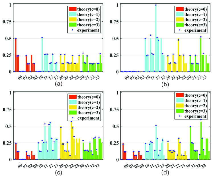
Figure 7: Probabilities corresponding to the decomposition of the witness $W^{\rm opt}$ when the measure-and-reprepare maps are projection on $|1\rangle$ and reset on (a) $|0\rangle$, (b) $|1\rangle$, (c) $|+\rangle$, and (d) $\frac{1}{\sqrt{2}}(|0\rangle+i|1\rangle)$. The data representation in this figure follows the same convention as in Fig. 6.

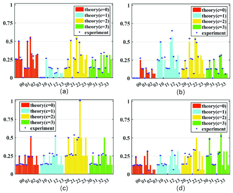
Figure 8: Probabilities corresponding to the decomposition of the witness $W^{\rm opt}$ when the measure-and-reprepare maps are projection on $|+\rangle$ and reset on (a) $|0\rangle$, (b) $|1\rangle$, (c) $|+\rangle$, and (d) $\frac{1}{\sqrt{2}}(|0\rangle+i|1\rangle)$. The data representation in this figure follows the same convention as in Fig. 6.

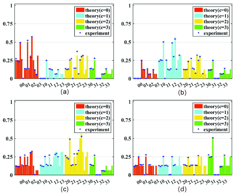
Figure 9: Probabilities corresponding to the decomposition of the witness $W^{\rm opt}$ when the measure-and-reprepare maps are projection on $\frac{1}{\sqrt{2}}(|0\rangle+i|1\rangle)$ and reset on (a) $|0\rangle$, (b) $|1\rangle$, (c) $|+\rangle$, and (d) $\frac{1}{\sqrt{2}}(|0\rangle+i|1\rangle)$. The data representation in this figure follows the same convention as in Fig. 6.

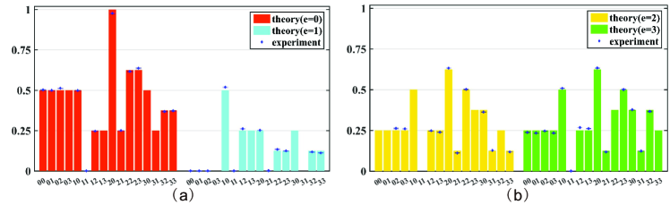
Figure 10: Probabilities of (a) the first 32 and (b) the next 32 terms in the decomposition of the experimentally friendly witness $W^{\prime}$. The dots represents the experimentally observed probabilities. The corresponding theoretical predictions shown in coloured bars (red, cyan, yellow, and green bars represent results when the target state is reprepared to $|0\rangle,|1\rangle,|+\rangle,\frac{1}{\sqrt{2}}(|0\rangle+i|1\rangle)$, respectively). The $x$ axis is labelled with the final measurement outcomes of the control qubit and switched measurement outcomes of the target qubit, ‘23’ means they are projected onto $|+\rangle,\frac{1}{\sqrt{2}}(|0\rangle+i|1\rangle)$ for example.

References

- Greaves and Thomas (2014) H. Greaves and T. Thomas, Studies in History and Philosophy of Science Part B: Studies in History and Philosophy of Modern Physics 45, 46 (2014).
- Aharonov et al. (1964) Y. Aharonov, P. G. Bergmann, and J. L. Lebowitz, Physical Review 134, B1410 (1964).
- Aharonov et al. (1990) Y. Aharonov, J. Anandan, S. Popescu, and L. Vaidman, Physical Review Letters 64, 2965 (1990).
- Aharonov and Vaidman (2002) Y. Aharonov and L. Vaidman, in Time in quantum mechanics (Springer, 2002) pp. 369–412.
- Abramsky and Coecke (2004) S. Abramsky and B. Coecke, in Proceedings of the 19th Annual IEEE Symposium on Logic in Computer Science, 2004. (IEEE, 2004) pp. 415–425.
- Hardy (2007) L. Hardy, Journal of Physics A: Mathematical and Theoretical 40, 3081 (2007).
- Oeckl et al. (2008) R. Oeckl et al., Advances in Theoretical and Mathematical Physics 12, 319 (2008).
- Svetlichny (2011) G. Svetlichny, International Journal of Theoretical Physics 50, 3903 (2011).
- Lloyd et al. (2011) S. Lloyd, L. Maccone, R. Garcia-Patron, V. Giovannetti, Y. Shikano, S. Pirandola, L. A. Rozema, A. Darabi, Y. Soudagar, L. K. Shalm, et al., Physical Review Letters 106, 040403 (2011).
- Genkina et al. (2012) D. Genkina, G. Chiribella, and L. Hardy, Physical Review A 85, 022330 (2012).
- Oreshkov and Cerf (2015) O. Oreshkov and N. J. Cerf, Nature Physics 11, 853 (2015).
- Silva et al. (2017) R. Silva, Y. Guryanova, A. J. Short, P. Skrzypczyk, N. Brunner, and S. Popescu, New Journal of Physics 19, 103022 (2017).
- Chiribella and Liu (2022) G. Chiribella and Z. Liu, Communications Physics 5, 1 (2022).
- Chiribella (2012) G. Chiribella, Physical Review A 86, 040301 (2012).
- Chiribella et al. (2013) G. Chiribella, G. M. D’Ariano, P. Perinotti, and B. Valiron, Physical Review A 88, 022318 (2013).
- Araújo et al. (2014a) M. Araújo, F. Costa, and Č. Brukner, Physical review letters 113, 250402 (2014a).
- Guérin et al. (2016) P. A. Guérin, A. Feix, M. Araújo, and Č. Brukner, Physical review letters 117, 100502 (2016).
- Ebler et al. (2018) D. Ebler, S. Salek, and G. Chiribella, Physical review letters 120, 120502 (2018).
- Zhao et al. (2020) X. Zhao, Y. Yang, and G. Chiribella, Physical Review Letters 124, 190503 (2020).
- Felce and Vedral (2020) D. Felce and V. Vedral, Physical review letters 125, 070603 (2020).
- Chiribella et al. (2021) G. Chiribella, M. Wilson, and H. Chau, Physical review letters 127, 190502 (2021).
- Procopio et al. (2015) L. M. Procopio, A. Moqanaki, M. Araújo, F. Costa, I. Alonso Calafell, E. G. Dowd, D. R. Hamel, L. A. Rozema, Č. Brukner, and P. Walther, Nature communications 6, 1 (2015).
- Rubino et al. (2017) G. Rubino, L. A. Rozema, A. Feix, M. Araújo, J. M. Zeuner, L. M. Procopio, Č. Brukner, and P. Walther, Science advances 3, e1602589 (2017).
- Goswami et al. (2018) K. Goswami, C. Giarmatzi, M. Kewming, F. Costa, C. Branciard, J. Romero, and A. G. White, Physical review letters 121, 090503 (2018).
- Wei et al. (2019) K. Wei, N. Tischler, S.-R. Zhao, Y.-H. Li, J. M. Arrazola, Y. Liu, W. Zhang, H. Li, L. You, Z. Wang, et al., Physical review letters 122, 120504 (2019).
- Guo et al. (2020) Y. Guo, X.-M. Hu, Z.-B. Hou, H. Cao, J.-M. Cui, B.-H. Liu, Y.-F. Huang, C.-F. Li, G.-C. Guo, and G. Chiribella, Phys. Rev. Lett. 124, 030502 (2020).
- Rubino et al. (2021a) G. Rubino, L. A. Rozema, D. Ebler, H. Kristjánsson, S. Salek, P. A. Guérin, A. A. Abbott, C. Branciard, Č. Brukner, G. Chiribella, et al., Physical Review Research 3, 013093 (2021a).
- Cao et al. (2022) H. Cao, N.-N. Wang, Z. Jia, C. Zhang, Y. Guo, B.-H. Liu, Y.-F. Huang, C.-F. Li, and G.-C. Guo, Physical Review Research 4, L032029 (2022).
- Nie et al. (2022) X. Nie, X. Zhu, K. Huang, K. Tang, X. Long, Z. Lin, Y. Tian, C. Qiu, C. Xi, X. Yang, et al., Physical Review Letters 129, 100603 (2022).
- Rubino et al. (2021b) G. Rubino, G. Manzano, and Č. Brukner, Communications Physics 4, 1 (2021b).
- Rubino et al. (2022) G. Rubino, G. Manzano, L. A. Rozema, P. Walther, J. M. Parrondo, and Č. Brukner, Physical Review Research 4, 013208 (2022).
- Chitambar and Gour (2019) E. Chitambar and G. Gour, Rev. Mod. Phys. 91, 025001 (2019).
- Gühne and Tóth (2009) O. Gühne and G. Tóth, Physics Reports 474, 1 (2009).
- Araújo et al. (2015) M. Araújo, C. Branciard, F. Costa, A. Feix, C. Giarmatzi, and Č. Brukner, New Journal of Physics 17, 102001 (2015).
- Milz et al. (2022) S. Milz, J. Bavaresco, and G. Chiribella, Quantum 6, 788 (2022).
- Landau and Streater (1993) L. Landau and R. Streater, Linear algebra and its applications 193, 107 (1993).
- Mendl and Wolf (2009) C. B. Mendl and M. M. Wolf, Communications in Mathematical Physics 289, 1057 (2009).
- Chiribella et al. (2008) G. Chiribella, G. M. D’Ariano, and P. Perinotti, EPL (Europhysics Letters) 83, 30004 (2008).
- Chiribella et al. (2009) G. Chiribella, G. M. D’Ariano, and P. Perinotti, Physical Review A 80, 022339 (2009).
- Åberg (2004a) J. Åberg, Annals of Physics 313, 326 (2004a).
- Åberg (2004b) J. Åberg, Physical Review A 70, 012103 (2004b).
- Oi (2003) D. K. Oi, Physical Review Letters 91, 067902 (2003).
- Zhou et al. (2011) X.-Q. Zhou, T. C. Ralph, P. Kalasuwan, M. Zhang, A. Peruzzo, B. P. Lanyon, and J. L. O’brien, Nature communications 2, 1 (2011).
- Soeda (2013) A. Soeda, in Talk at the Int. Conf. Quantum Information and Technology (ICQIT2013), Tokyo, Japan, Vol. 1618 (2013).
- Araújo et al. (2014b) M. Araújo, A. Feix, F. Costa, and Č. Brukner, New Journal of Physics 16, 093026 (2014b).
- Friis et al. (2014) N. Friis, V. Dunjko, W. Dür, and H. J. Briegel, Physical Review A 89, 030303 (2014).
- Gavorová et al. (2020) Z. Gavorová, M. Seidel, and Y. Touati, arXiv preprint arXiv:2011.10031 (2020).
- Thompson et al. (2018) J. Thompson, K. Modi, V. Vedral, and M. Gu, New Journal of Physics 20, 013004 (2018).
- Dong et al. (2019) Q. Dong, S. Nakayama, A. Soeda, and M. Murao, arXiv preprint arXiv:1911.01645 (2019).
- Gisin et al. (2005) N. Gisin, N. Linden, S. Massar, and S. Popescu, Physical Review A 72, 012338 (2005).
- Abbott et al. (2020) A. A. Abbott, J. Wechs, D. Horsman, M. Mhalla, and C. Branciard, Quantum 4, 333 (2020).
- Chiribella and Kristjánsson (2019) G. Chiribella and H. Kristjánsson, Proceedings of the Royal Society A 475, 20180903 (2019).
- Kristjánsson et al. (2021) H. Kristjánsson, W. Mao, G. Chiribella, et al., Physical Review Research 3, 043147 (2021).
- Kristjánsson et al. (2020) H. Kristjánsson, G. Chiribella, S. Salek, D. Ebler, and M. Wilson, New Journal of Physics 22, 073014 (2020).
- Lamoureux et al. (2005) L.-P. Lamoureux, E. Brainis, N. Cerf, P. Emplit, M. Haelterman, and S. Massar, Physical review letters 94, 230501 (2005).
- Choi (1975) M.-D. Choi, Linear algebra and its applications 10, 285 (1975).
- Steiner (2003) M. Steiner, Physical Review A 67, 054305 (2003).
- Nesterov and Nemirovskii (1994) Y. Nesterov and A. Nemirovskii, Interior-point polynomial algorithms in convex programming (SIAM, 1994).
- Oreshkov and Giarmatzi (2016) O. Oreshkov and C. Giarmatzi, New Journal of Physics 18, 093020 (2016).