Model-Free Learning of Optimal Beamformers for
Passive IRS-Assisted Sumrate Maximization

Abstract

Although Intelligent Reflective Surfaces (IRSs) are a cost-effective technology promising high spectral efficiency in future wireless networks, obtaining optimal IRS beamformers is a challenging problem with several practical limitations. Assuming fully-passive, sensing-free IRS operation, we introduce a new data-driven Zeroth-order Stochastic Gradient Ascent (ZoSGA) algorithm for sumrate optimization in an IRS-aided downlink setting. ZoSGA does not require access to channel model or network structure information, and enables learning of optimal long-term IRS beamformers jointly with standard short-term precoding, based only on conventional effective channel state information. Supported by state-of-the-art (SOTA) convergence analysis, detailed simulations confirm that ZoSGA exhibits SOTA empirical behavior as well, consistently outperforming standard fully model-based baselines, in a variety of scenarios.

Index Terms— Intelligent Reflecting Surfaces, Sumrate Maximization, Zeroth-order Optimization, Model-Free Learning.

1 Introduction

Intelligent Reflective (or Reconfigurable Intelligent) Surfaces (IRSs or RISs) are planar surfaces comprised of passive reflective elements with tunable phase-shifts and amplitudes. Seen as beamforming arrays, IRSs present a promising solution to mitigate sharp drops in Quality-of-Service (QoS) in the absence of line of sight for highly directional mmWave signals, and beyond. Such a typical scenario is visualized in Fig. 1, where users linked with an Access Point (AP) are enjoying improved QoS due to the IRSs assisting the network.

In IRS-aided communications, the goal is to optimally tune the IRS elements along with other possible resources (such as AP precoders) to optimize a certain system utility. A standard case is that of the weighted sumrate utility in a MISO downlink scenario (see Fig. 1), where the goal is to maximize the total downlink rate of a number of users (i.e., terminals) actively serviced by an AP, while passively aided by one or multiple IRSs. Then, the objective is to jointly optimize IRS amplitudes/phase-shifts and AP precoders, subject to certain power constraints. While AP precoders are usually continuous-valued, IRS phase-shifts can be either quantized [1] or continuously varying [2, 3]. In this paper, we focus on the latter, i.e., on optimizing for continuous IRS phase-shift variations, however strictly assuming fully-passive IRS elements with no sensing capabilities or extra hardware or scheduling requirements.

Recently, various deep learning driven methods have been proposed for IRS-aided beamforming optimization. Offline learning approaches have been proposed primarily to estimate the Channel State Information (CSI) using labeled datasets with Function Approximators (FAs) [4, 5, 6, 7]. In contrast, Deep Reinforcement Learning (DRL) methods have been used for joint beamforming optimization, either with quantized [8, 9, 10] or continuous [11, 12] actions. Though such end-to-end DRL methods do not require intermediate CSI estimates or active IRS sensing, they do require FAs to at least approximate value functions, jointly modeling the whole optimization task, including beamforming controllers. On the one hand, choosing such FAs without explicit domain knowledge usually results in increased problem complexity, non-interpretability and lack of robustness, whereas incorporating specific domain knowledge often results in overfitting, hindering versatility and transferability to distinct environments. Further, as such approaches primarily consider reactive IRS tuning (i.e., phase shifts depend on observed CSI), they naturally incur increased power consumption for perpetual IRS control.

Fig. 1: Realization/Concept of an IRS-aided Wireless Network.

To improve complexity, efficiency and robustness, model-based two-timescale approaches have also been proposed, in which reactive (AP) precoding is combined with static (i.e., non-reactive) IRS beamforming [13, 14, 15, 16, 17]. Although potentially effective, such methods rely on optimizing problem surrogates and leverage detailed knowledge of channel models and spatial network configurations, often requiring active sensing at the IRSs. Thus, they are not applicable to different settings without complete remodeling of the environment.

In this paper, we develop a new Zeroth-order Stochastic Gradient Ascent (ZoSGA) two-timescale algorithm for weighted sumrate optimization in the MISO downlink setting through purely data-driven learning of optimal IRS beamformers, and joint reactive AP precoding via the standard WMMSE algorithm [18]. ZoSGA follows the two-timescale paradigm while being completely FA- and model-free, and relies on minimal zeroth-order reinforcement (i.e., system probing), as well as user-experienced effective CSI (see Section 2), conventionally available in mutli-user downlink beamfoming, regardless of the number or spatial configuration of the IRSs. In fact, ZoSGA allows treating the IRSs assisting the network as fully passive (though tunable) reflecting elements, and applies to different networking scenarios seamlessly.

We analyze ZoSGA under mild regularity conditions and establish a state-of-the-art (SOTA) convergence rate of order $\mathcal{O}(\sqrt{S}\epsilon^{-4})$, where $S$ is the number of IRS tunable parameters and $\epsilon$ is the suboptimality target. Then, we numerically demonstrate that ZoSGA also achieves SOTA empirical performance in a variety of scenarios, substantially outperforming the two-timescale method of [14], which is a standard model-based baseline for the problem under study, assuming full knowledge of the underlying channel model and spatial network configuration. Overall, ZoSGA sets a new SOTA for beamforming optimization in IRS-aided communications.

Note: Proofs are omitted due to lack of space and will be included in a journal paper currently under preparation. Fully reproducible code is available at github.com/hassaanhashmi/zosga-irs.

2 Problem Formulation

Capitalizing on the standardized IRS-Aided communication setting depicted in Fig. 1, our goal is to maximize the total downlink rate of $K$ users actively serviced by an AP with $M$ antennas, while passively aided by one or multiple IRSs, arbitrarily spatially placed. As explained in Section 1, we assume dynamic (i.e., reactive) AP beamformers (also called precoders), while the IRS beamformers are realistically viewed as static (i.e., non-reactive) elements, tunable by a parameter vector $\bm{\theta}\in\mathbb{R}^{S}$, encompassing whatever propagation feature is learnable on the IRSs present in the network. For instance, $\bm{\theta}$ might refer to amplitudes, phases, or both, or even realistic physical elements of an IRS, such as tunable varactor capacitance elements, see, e.g., [2, 3]. We strictly make no sensing assumptions on the IRSs, i.e., the IRSs are completely passive network elements.

Each user $k=1,\ldots,K$ experiences a random effective channel denoted by $\mathbf{h}_{k}\left(\bm{\theta},\omega\right)$, indexed by the IRS parameter vector $\bm{\theta}$ as well as a state of nature $\omega\in\Omega$ describing unobservable random propagation patterns for each value of $\bm{\theta}$. In other words, $\mathbf{h}_{k}\left(\bm{\theta},\omega\right)$ is a random channel field with spatial variable $\bm{\theta}$. We make the standard assumption that the effective channels $\mathbf{h}_{k}\left(\bm{\theta},\omega\right),k=1,\ldots,K$ are known to the AP at the time of transmission [13, 14]. Note that the implementation complexity of estimating effective channels in our setting is exactly the same as that in conventional multi-user downlink beamforming (i.e., involving no IRSs), regardless of the number and/or spatial configuration of the IRSs; no extra hardware or customized scheduling schemes (such as those in [14]) are required on either the AP or the IRSs assisting the network.

The QoS of user $k$ is measured by the corresponding SINR, i.e.,

$$\begin{aligned} \text{SINR}_{k}(\mathbf{W},\mathbf{h}_{k}(\bm{\theta},\omega))\triangleq\frac{\left|\mathbf{h}_{k}^{\mathsf{H}}(\bm{\theta},\omega)\mathbf{w}_{k}\right|^{2}}{{\sum}_{{j\in\mathbb{N}_{K}^{+}\setminus k}}\left|\mathbf{h}^{\mathsf{H}}_{k}(\bm{\theta},\omega)\mathbf{w}_{j}\right|^{2}+\sigma^{2}_{k}},\end{aligned}$$

where $\mathbf{W}{=}\begin{bmatrix}\mathbf{w}_{1}&\mathbf{w}_{2}&\cdots&\mathbf{w}_{K}\end{bmatrix}\in\mathbb{C}^{M\times K}$, $\mathbf{w}_{k}$ is a transmit precoding vector and $\sigma^{2}_{k}$ is the noise variance for user $k$, respectively. Then, the weighted sumrate utility of the network is defined as

$${F}(\mathbf{W},\mathbf{H}(\bm{\theta},\omega))\triangleq\sum_{k=1}^{K}\alpha_{k}\log_{2}\left(1+\textnormal{SINR}_{k}\left(\mathbf{w},\mathbf{h}_{k}\left(\bm{\theta},\omega\right)\right)\right),$$

with $\mathbf{H}=\begin{bmatrix}\mathbf{h}_{1}\ldots\mathbf{h}_{K}\end{bmatrix}\in\mathbb{C}^{M\times K}$, and $\alpha_{k}\geq 0$ the weight associated with user $k$. We are interested in maximizing the sumrate of the network jointly by selecting instantaneous-optimal dynamic AP precoders $\mathbf{W}$, and on-average-optimal static IRS beamformers $\bm{\theta}$ [13, 14], i.e., we are interested in the problem

$$\boxed{\max_{\bm{\theta}\in\mathcal{K}}\mathbb{E}\bigg{\{}\max_{\mathbf{W}:\|\mathbf{W}\|_{F}^{2}\leq P}{F}\left(\mathbf{W},\mathbf{H}(\bm{\theta},\omega)\right)\bigg{\}},}$$ (1)

where $\|\cdot\|_{F}^{2}$ denotes the Frobenius norm, $P>0$ is a total power budget at the AP, and $\mathcal{K}$ is a compact feasible set. Problem (1) is an instance of a $2$-stage stochastic program [19]. Accordingly, we may interpret optimization over $\bm{\theta}$ as the first-stage problem, where the decision-maker optimizes the IRS parameters on-average and before the actual effective channels are revealed, whereas optimization over $\mathbf{W}$ constitutes the second stage problem which is solved after randomness is revealed to the decision-maker, therefore interpreting optimal AP beamforming as (optimal) recourse actions.

$$\begin{aligned} \bm{D}(\mathbf{W},\mathbf{H}(\bm{\theta},\omega))=\sum_{k=1}^{K}\alpha_{k}\frac{\mathbf{z}^{\mathsf{H}}\left[\left(\sum_{j\in\mathbb{N}_{K}^{+}\setminus k}\left|\mathbf{z}^{\mathsf{H}}\mathbf{w}_{j}\right|^{2}+\sigma^{2}_{k}\right)\mathbf{w}_{k}{\mathbf{w}_{k}}^{\mathsf{H}}-\left|\mathbf{z}^{\mathsf{H}}\mathbf{w}_{k}\right|^{2}\sum_{j\in\mathbb{N}_{K}^{+}\setminus k}\mathbf{w}_{j}{\mathbf{w}_{j}}^{\mathsf{H}}\right]}{\ln(2)(\sum_{j\in\mathbb{N}_{K}^{+}\setminus k}|\mathbf{z}^{\mathsf{H}}\mathbf{w}_{j}|^{2}+\sigma^{2}_{k})^{2}+|\mathbf{z}^{\mathsf{H}}\mathbf{w}_{k}|^{2}(\sum_{j\in\mathbb{N}_{K}^{+}\setminus k}|\mathbf{z}^{\mathsf{H}}\mathbf{w}_{j}|^{2}+\sigma^{2}_{k})}\Bigg{|}_{\mathbf{z}=\mathbf{H}(\bm{\theta},\omega)}.\end{aligned}$$ (D)

$$\begin{aligned} \dfrac{\mathbf{G}_{\mu}(\bm{\theta},\omega,\mathbf{u})}{2}\triangleq&\left(\frac{\Re\left(\mathbf{\Delta}_{\mu}(\bm{\theta},\omega,\mathbf{u})\right)}{2\mu}\mathbf{u}^{\mathsf{T}}\right)^{\mathsf{T}}\left(\Re\left(\bm{D}(\mathbf{W}^{*},\mathbf{H}(\bm{\theta},\omega))\right)\right)^{\mathsf{T}}+\left(\frac{\Im\left(\mathbf{\Delta}_{\mu}(\bm{\theta},\omega,\mathbf{u})\right)}{2\mu}\mathbf{u}^{\mathsf{T}}\right)^{\mathsf{T}}\left(\Re\left(j\bm{D}(\mathbf{W}^{*},\mathbf{H}(\bm{\theta},\omega))\right)\right)^{\mathsf{T}}.\end{aligned}$$ (G)

3 An inner-outer optimization method

We would like to devise a gradient-inspired method for tackling problem (1), which circumvents the need for accessing first-order gradient information of the effective channel function $\mathbf{H}(\cdot,\omega)$; in principle, this is unknown. To that end, we derive an inner-outer scheme for the solution of the two-stage problem in (1). At each (outer) iteration (i.e., for each state of nature $\omega$), we employ an oracle to find an approximate solution to the inner problem, which is then utilized to derive a model-free gradient approximation for the outer problem using zeroth-order reinforcement (i.e., probing) on the involved effective channel. This approach completely bypasses the need of a model for the effective channel, and offers great flexibility as to how the inner problem can be approximately solved.

3.1 Tackling the Inner Problem (AP Precoding)

To obtain an approximate solution for the (nonconvex) inner maximization problem, we heuristically employ the well-known weighted minimum mean squared error (WMMSE) algorithm [18], simultaneously implementing AP precoding. For technical purposes, we also introduce the following assumption.

Assumption 1.

Given any $\bm{\theta}\in\mathcal{K}$ and almost every (a.e.) $\omega\in\Omega$, we have access to an oracle that yields an optimal solution $\bm{W}^{*}(\bm{\theta},\omega)\in\arg\max_{\mathbf{W}\colon\|\mathbf{W}\|_{F}^{2}\leq P}{F}(\mathbf{W},\mathbf{H}(\bm{\theta},\omega))$.

In practice Assumption 1 may be restrictive but, as verified in Section 5, the empirical effectiveness of the proposed algorithm is not hindered. Nevertheless, this assumption is crucial for the derivation of our algorithm and its subsequent theoretical analysis.

3.2 Tackling the Outer Problem (IRS Beamforming)

Assuming the availability of an oracle providing an optimal solution to the inner problem at any $(\bm{\theta},\omega)$, say $\mathbf{W}^{*}(\bm{\theta},\omega)$ (in practice obtained approximately via WMMSE), we can write problem (1) as

$$\begin{split}\max_{\bm{\theta}\in\mathcal{K}}&\ \mathbb{E}\left\{{F}\left(\mathbf{W}^{*}(\bm{\theta},\omega),\mathbf{H}(\bm{\theta},\omega)\right)\right\}.\end{split}$$ (2)

As we would like to derive a gradient-ascent-like scheme for solving (2), let us make the following assumptions on the effective channel.

Assumption 2.

For almost all $\omega$, the channel function $\mathbf{H}(\cdot,\omega)$ is uniformly bounded, twice continuously-differentiable, $L_{\mathbf{h},0}$-Lipschitz, with $L_{\mathbf{h},1}$-Lipschitz gradients.

We note that Assumption 2 imposes regularity conditions mainly required for the grounded development of our optimization scheme and for its convergence analysis (later in Section 4). Also, observe that the boundedness assumption is natural, since (IRS-aided) wireless channels are always bounded in practice. While we usually have no information on the analytical properties of the effective channel, Assumption 2 is easily satisfied in widely used channel models of IRS-aided systems, see, e.g., [14] as well as Section 5.

From Assumptions 1–2, and the compactness of $\mathcal{K}$, we obtain

$$\begin{split}&\nabla_{\bm{\theta}}\mathbb{E}\left\{{F}\left(\mathbf{W}^{*}(\bm{\theta},\omega),\mathbf{H}(\bm{\theta},\omega)\right)\right\}\\ &\quad=\mathbb{E}\left\{\nabla_{\bm{\theta}}{F}\left(\mathbf{W}^{*}(\bm{\theta},\omega),\mathbf{H}(\bm{\theta},\omega)\right)\right\}\\ &\quad=\mathbb{E}\left\{\nabla_{\bm{\theta}}{F}\left(\mathbf{W},\mathbf{H}\left(\bm{\theta},\omega\right)\right)\mid_{\mathbf{W}=\mathbf{W}^{*}(\bm{\theta},\omega)}\right\},\end{split}$$ (3)

where we used [19, Theorem 7.44], and the implicit function theorem (e.g., see [20]). Next, we derive the gradient of ${F}(\mathbf{W},\mathbf{H}(\cdot,\omega))$.

3.2.1 Gradient Representation for the Outer Problem

We notice that ${F}(\mathbf{W},\cdot)$ takes a complex input and hence we need an appropriate generalization of the gradient for it. To that end, we utilize the so-called Wirtinger calculus (see [21]). In the following lemma we derive the full compositional gradient of ${F}(\mathbf{W},\mathbf{H}(\bm{\theta},\omega))$ by following the developments in [21, Section 4].

Lemma 1.

For every $\bm{\theta}\in\mathcal{K}$, $\mathbf{W}\in\mathbb{C}^{M\times K}$ and $\omega\in\Omega$, the gradient of ${F}\left(\mathbf{W},\mathbf{H}(\bm{\theta},\omega)\right)$ with respect to $\bm{\theta}$ reads

$$\begin{split}\nabla_{\bm{\theta}}&{F}\left(\mathbf{W},\mathbf{H}(\bm{\theta},\omega)\right)\\ &\quad=2\nabla_{\bm{\theta}}\Re\left(\mathbf{H}(\bm{\theta},\omega)\right)\left(\Re\left(\bm{D}\left(\mathbf{W},\mathbf{H}(\bm{\theta},\omega)\right)\right)\right)^{\mathsf{T}}\\ &\qquad+2\nabla_{\bm{\theta}}\Im\left(\mathbf{H}(\bm{\theta},\omega)\right)\left(\Re\left(j\bm{D}\left(\mathbf{W},\mathbf{H}(\bm{\theta},\omega)\right)\right)\right)^{\mathsf{T}},\end{split}$$

where $\bm{D}(\mathbf{W},\mathbf{H}(\bm{\theta},\omega))$ is given in (D). Additionally, there exists a constant $B_{F}>0$ such that $\left\|\bm{D}(\mathbf{W},\mathbf{H}(\bm{\theta},\omega))\right\|\leq B_{F}$ for every $(\mathbf{W},\bm{\theta})\in\mathbb{C}^{M\times K}\times\mathcal{K}$ and a.e. $\omega\in\Omega$, where $\mathbf{W}$ is feasible for (1).

3.2.2 Model-Free Jacobian Approximation of the Effective Channel

Assuming the lack of availability of any first-order information of $\mathbf{H}(\cdot,\omega)$ for any $\omega\in\Omega$, we will employ a zeroth-order scheme in order to obtain a Jacobian estimate of $\nabla_{\bm{\theta}}\mathbf{H}(\bm{\theta},\omega)$, using which we can solve (2) via a stochastic gradient ascent scheme. The proposed method will be based on Jacobian estimates arising from a two-point stochastic evaluation of $\mathbf{H}(\cdot,\omega)$ (similar to, among others, [22, 23, 24]). From Assumption 2, we can first write

$$\nabla_{\bm{\theta}}\mathbf{H}(\bm{\theta},\omega)=\nabla_{\bm{\theta}}\Re\left(\mathbf{H}(\bm{\theta},\omega)\right)+j\nabla_{\bm{\theta}}\Im\left(\mathbf{H}(\bm{\theta},\omega)\right).$$

We approximate this gradient using only function evaluations of $\mathbf{H}(\cdot,\omega)$ (i.e. by minimally probing the network). For each $\omega\in\Omega$, let $\mathbf{u}\sim\mathcal{N}\left(\mathbf{0},\mathbf{I}\right)$. Given a smoothing parameter $\mu>0$, we define

$$\begin{split}\nabla^{\mu}_{\bm{\theta}}\mathbf{H}(\bm{\theta},\omega)\triangleq&\ \mathbb{E}\left\{\frac{\mathbf{H}\left(\bm{\theta}+\mu\mathbf{u},\omega\right)-\mathbf{H}\left(\bm{\theta}-\mu\mathbf{u},\omega\right)}{2\mu}\mathbf{u}^{\mathsf{T}}\right\}^{\mathsf{T}}.\end{split}$$ (4)

Using Lemma 1, we substitute the Jacobian of the effective channel via the zeroth-order approximation given in (4) to obtain the zeroth-order compositional quasi-gradient (an approximation of (2)) as

$$\begin{split}{\hat{\nabla}}_{\bm{\theta}}^{\mu}&{F}\left(\mathbf{W}^{*},\mathbf{H}(\bm{\theta},\omega)\right)\\ &\quad=2\nabla^{\mu}_{\bm{\theta}}\Re\left(\mathbf{H}(\bm{\theta},\omega)\right)\left(\Re\left(\bm{D}\left(\mathbf{W}^{*},\mathbf{H}(\bm{\theta},\omega)\right)\right)\right)^{\mathsf{T}}\\ &\qquad+2\nabla^{\mu}_{\bm{\theta}}\Im\left(\mathbf{H}(\bm{\theta},\omega)\right)\left(\Re\left(j\bm{D}\left(\mathbf{W}^{*},\mathbf{H}(\bm{\theta},\omega)\right)\right)\right)^{\mathsf{T}}.\end{split}$$

We are now able to derive the proposed inner-outer scheme for the solution of problem (1). At every iteration $t$, we draw independent and identically distributed (i.i.d.) samples $\omega^{t+1}$ and $\mathbf{u}^{t+1}$, and compute an “optimal" inner solution $\mathbf{W}^{*}(\bm{\theta}^{t},\omega^{t+1})$, as described in Section 3.1. Then, by probing the system twice, we can compute a zeroth-order stochastic gradient estimator as shown in (G), where $\mathbf{\Delta}_{\mu}(\bm{\theta},\omega,\mathbf{u})\triangleq\mathbf{H}(\bm{\theta}+\mu\mathbf{u},\omega)-\mathbf{H}(\bm{\theta}-\mu\mathbf{u},\omega)$. The proposed Zeroth-order Stochastic Gradient Ascent (ZoSGA) method with WMMSE is provided in Algorithm 1.

1 Initialize $\mathbf{W}^{0}$, $\bm{\theta}^{0}$, $\eta^{0}$, $\mu$.

2 for $t=0,\ldots,T$ do

3     Sample (i.i.d.) $(\mathbf{u}^{t+1},\omega^{t+1})$.

4     Find $\mathbf{W}^{*}(\bm{\theta}^{t},\omega^{t+1})$ using WMMSE [18].

5     Compute $\mathbf{G}_{\mu}(\bm{\theta}^{t},\omega^{t+1},\mathbf{u}^{t+1})$ using (G) (by probing).

6     Choose $\eta^{t+1}$ and update

$$\bm{\theta}^{t+1}=\Pi_{\mathcal{K}}\left(\bm{\theta}^{t}+\eta^{t+1}\mathbf{G}_{\mu}(\bm{\theta}^{t},\omega^{t+1},\mathbf{u}^{t+1})\right),$$

     where $\Pi_{\mathcal{K}}(\cdot)$ is the Euclidean projection onto $\mathcal{K}$.

7  end for

Return $\bm{\theta}^{t^{*}}$, where $\mathbb{P}(t^{*}=t)=\frac{\eta^{n}}{\sum_{i=0}^{T}\eta^{i}}$.

Algorithm 1 ZoSGA with WMMSE

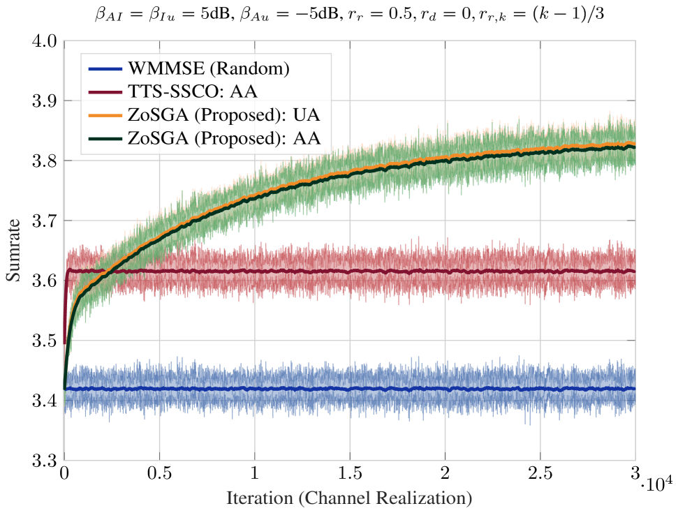
(a)

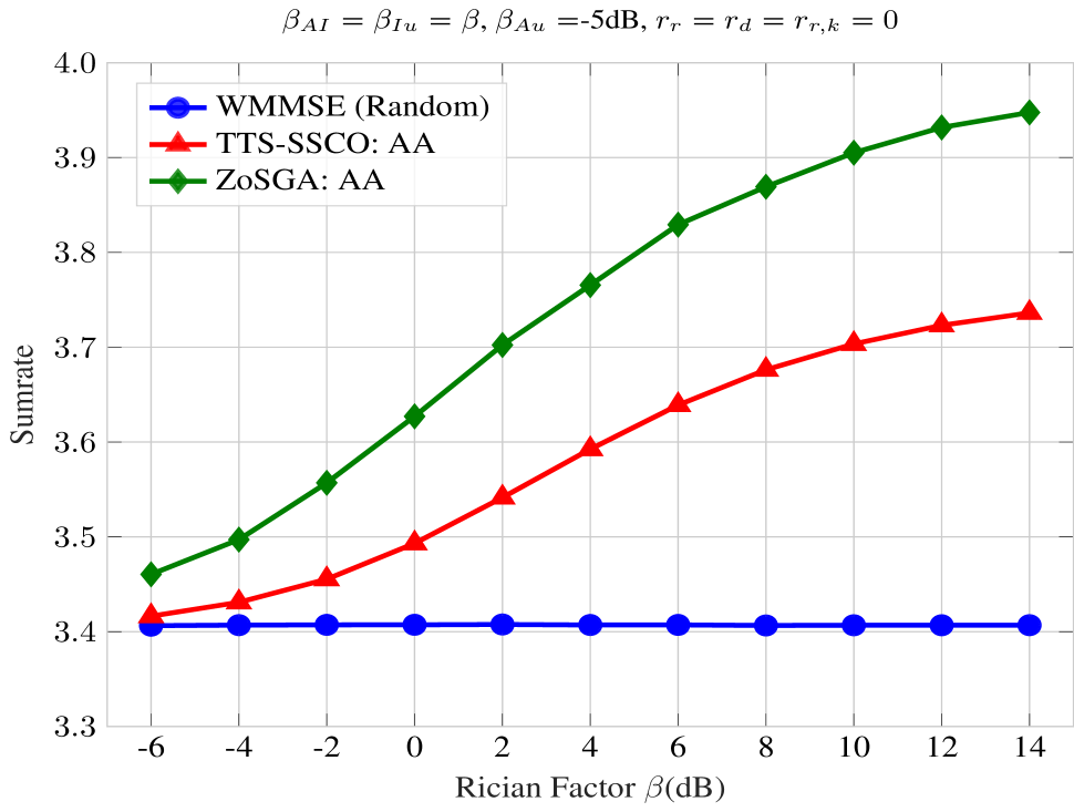
(b)

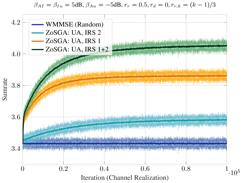
(c)

Fig. 2: Average sumrates achieved by WMMSE [18] (with random IRS phase shifts), TTS-SSCO [14], and the proposed ZoSGA algorithm, with only IRS 1 present: (a) with fixed parameters $\beta_{*}$ and $r_{*}$, and (b) relative to Rician factors $\beta_{AI}=\beta_{Iu}$; (c) Average sumrates achieved by WMMSE and ZoSGA with IRS 1+2 present and fixed parameters $\beta_{*}$ and $r_{*}$. (AA: Adjustable Amplitude; UA: Unit Amplitude)

4 Convergence analysis

In this section we provide a brief account of the convergence properties of Algortithm 1. For convenience let $\varphi(\cdot)\triangleq-\mathbb{E}\{F_{\omega}^{*}(\cdot)\}+\delta_{\mathcal{K}}(\cdot)$, where $F_{\omega}^{*}(\cdot)\triangleq F\left(\mathbf{W}^{*}(\cdot,\omega),\mathbf{H}(\cdot,\omega)\right)$ is the (sample) objective of problem (2) and $\delta_{\mathcal{K}}(\cdot)\in\{0,\infty\}$ is the indicator of the set $\mathcal{K}$. The following lemma is crucial for the analysis of Algorithm 1.

Lemma 2.

Let Assumptions 1, 2 be in effect, and let $\widehat{\mathcal{K}}\supset\mathcal{K}$ be a convex compact set. Then, for a.e. $\omega$ there exists $\rho(\omega)>0$ such that $-F_{\omega}^{*}$ is $\rho(\omega)$-weakly convex on $\widehat{\mathcal{K}}$, i.e., $-F_{\omega}^{*}(\cdot)+(\rho(\omega)/2)\|\cdot\|^{2}$ is convex on $\widehat{\mathcal{K}}$.

Given some $\lambda>0$, we define the Moreau envelope of $\varphi$ as

$$\varphi^{\lambda}(\bm{y})\triangleq\min_{\bm{\theta}}\left\{\varphi(\bm{\theta})+\frac{1}{2\lambda}\|\bm{y}-\bm{\theta}\|^{2}\right\}.$$

A near-stationary point for the Moreau envelope $\varphi^{\lambda}$ is close to a near-stationary solution of problem (1), if $-\mathbb{E}\{F_{\omega}^{*}(\cdot)\}$ is weakly convex (see [25, Section 2.2] and note, from Lemma 2, that $-\mathbb{E}\{F_{\omega}^{*}(\cdot)\}$ is weakly convex if $\rho(\omega)$ is integrable). In what follows, we provide a convergence rate of Algorithm 1 in terms of the gradient of the Moreau envelope.

Theorem 3.

Let Assumptions 1, 2 be in effect and assume that $\mathcal{K}$ is convex and compact, $\rho=\mathbb{E}\{\rho(\omega)\}<\infty$, while the process $\{\omega^{t}\}_{t\in\mathbb{N}}$ is i.i.d.. Let $\{\bm{\theta}^{t}\}_{t=0}^{T}$ be the sequence of iterates generated by Algorithm 1, $\Delta_{\mathcal{K}}>0$ be the diameter of $\mathcal{K}$, and set

$$\eta^{t}=\sqrt{\frac{\Delta_{\varphi}}{4\rho B_{F}^{2}L_{\mathbf{h},0}^{2}(S^{2}+2S)(T+1)}},\qquad\textnormal{for all }t\geq 0,$$

for some $\Delta_{\varphi}\geq\varphi^{1/(2\rho)}(\bm{\theta}^{0})-\min_{\bm{\theta}}\varphi(\bm{\theta})$. Then, it is true that

$$\begin{split}&\mathbb{E}\big{\{}\big{\|}\nabla\varphi^{1/(2\rho)}\big{(}\bm{\theta}^{t^{*}}\big{)}\big{\|}^{2}_{2}\big{\}}\\ &\leq\ 8\Bigg{(}\sqrt{\frac{\Delta_{\varphi}\rho B_{F}^{2}L_{\mathbf{h},0}^{2}(S^{2}+2S)}{T+1}}+\mu\rho\Delta_{\mathcal{K}}B_{F}L_{\mathbf{h},1}\sqrt{SMK}\Bigg{)}.\end{split}$$

Remark 1.

Note that choosing $\mu=\mathcal{O}(1/\sqrt{(MKT)})$ yields that $\mathbb{E}\big{\{}\big{\|}\nabla\varphi^{1/(2\rho)}\big{(}\bm{\theta}^{t^{*}}\big{)}\big{\|}_{2}\big{\}}\leq\epsilon$, after $\mathcal{O}(\sqrt{S}\epsilon^{-4})$ iterations.

5 Simulations

We consider an IRS-aided MISO downlink wireless network with Rician fading channels $\mathbf{G}_{i}\in\mathbb{C}^{N{\times}M}$, $\mathbf{h}^{i}_{r,k}\in\mathbb{C}^{N}$ and $\mathbf{h}_{d,k}\in\mathbb{C}^{M}$, respectively, as shown in Fig. 3, where $i\in\{1,2\}$. Following [14], these channels are defined for each user $k$ as

$$\begin{aligned} \mathbf{h}_{r,k}^{i}&{\triangleq}\sqrt{\beta_{Iu}{/}(1{+}\beta_{Iu})}\check{\mathbf{v}}^{i}_{r,k}{+}\sqrt{1{/}(1{+}\beta_{Iu})}\mathbf{\Phi}_{r,k}^{1/2}\mathbf{v}_{r,k}^{i},\\ \mathbf{G}_{i}&{\triangleq}\sqrt{\beta_{AI}{/}(1{+}\beta_{AI})}\check{\mathbf{F}}^{i}{+}\sqrt{1{/}(1{+}\beta_{AI})}\mathbf{\Phi}_{r}^{1/2}\mathbf{F}^{i}\mathbf{\Phi}_{d}^{1/2},\\ \mathbf{h}_{d,k}&{\triangleq}\sqrt{\beta_{Au}{/}(1{+}\beta_{Au})}\check{\mathbf{v}}_{d,k}{+}\sqrt{1{/}(1{+}\beta_{Au})}\mathbf{\Phi}_{d}^{1/2}\mathbf{v}_{d,k},\\ \end{aligned}$$ (5)

where the entries of $\mathbf{H}_{\text{S-CSI}}{\triangleq}\{\check{\mathbf{v}}^{i}_{r,k}{,}\check{\mathbf{F}}^{i}{,}\check{\mathbf{v}}_{d,k}\}$ and $\mathbf{H}_{\text{I-CSI}}{\triangleq}$ $\{\mathbf{v}^{i}_{r,k}{,}\mathbf{F}^{i}{,}$ $\mathbf{v}_{d,k}\}$ ($i\in\{1,2\}$) are all sampled independently from $\mathcal{CN}(\bf{0},\bf{I})$, with the former being sampled only once per simulation, where a simulation is defined as an ensemble containing a number of sequential i.i.d. realizations of "instantaneous" CSI $\mathbf{H}_{\text{I-CSI}}$ (given a fixed value for "statistical" CSI $\mathbf{H}_{\text{S-CSI}}$ for each simulation).

Each IRS has $N{=}N_{h}{\times}N_{v}$ phase-shift elements (see Fig. 3). Thus, $\bm{\theta}_{i}{=}\begin{bmatrix}\bm{\phi}_{i}^{\mathsf{T}}&\mathbf{A}_{i}^{\mathsf{T}}\end{bmatrix}^{\mathsf{T}}$, where $\bm{\phi}_{i}\in[-\pi,\pi]^{N}$ and $\mathbf{A}_{i}\in[0,1]^{N}$ are phases and amplitudes of the IRS elements, respectively, with $i\in\{1,2\}$. The scalars $\beta_{Iu}$, $\beta_{AI}$, and $\beta_{Au}$, are link-specific Rician factors, while $\mathbf{\Phi}_{r,k}\in\mathbb{C}^{N{\times}N}$, $\mathbf{\Phi}_{r}\in\mathbb{C}^{N{\times}N}$ and $\mathbf{\Phi}_{d}\in\mathbb{C}^{M{\times}M}$ are spatial correlation matrices following the exponentially decaying correlation model of [14, 15], with corresponding correlation coefficients $r_{r,k}\in(0,1)$, $r_{r}\in(0,1)$ and $r_{d}\in(0,1)$. Lastly, the distance-dependent path-loss for each link is modeled as $L=\sqrt{C_{0}{d}^{-\alpha}}$, where $d$ is distance (in meters), $\alpha$ is the corresponding path loss exponent, and $C_{0}{=}$-30dBm.

Throughout the simulations we consider a power allocation of $P{=}$5dBm, a noise variance $\sigma^{2}{=}$ -80dBm, and run WMMSE for 20 iterations to optimize the precoding vectors $\mathbf{W}$ for each instance of the received effective channels $\mathbf{h}_{k}(\bm{\theta},\omega)$, each of which is given as

$$\mathbf{h}_{k}(\bm{\theta},\mathbf{\omega})=\sum_{i=1}^{2}\underbrace{\mathbf{G}^{\mathsf{H}}_{i}\text{diag}(\mathbf{A}_{i}\circ e^{-j{\bm{\phi}}_{i}})\mathbf{h}^{i}_{r,k}}_{\bm{\theta}_{i}\text{-reflected link}}+\underbrace{\mathbf{h}_{d,k}}_{\text{LoS link}},$$ (6)

for all $k\in\mathbb{N}^{+}_{4}$, where $\bm{\theta}{=}(\bm{\theta}_{1},\bm{\theta}_{2})$, $\omega=\{\mathbf{G}_{1},\mathbf{G}_{2},\mathbf{h}^{1}_{r,k},\mathbf{h}^{2}_{r,k},\mathbf{h}_{d,k},$ $k=1,\ldots,K\}$ and, for simplicity, we ignore IRS-to-IRS links. All presented results are averaged over 2000 unique simulations.

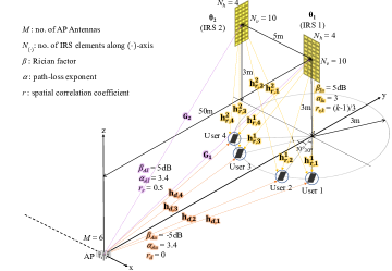
Fig. 3: Experimental IRS-Aided Network Configuration.

First, we compare the proposed ZoSGA against TTS-SSCO [14] for a network with one IRS as TTS-SSCO requires an exact model to optimize the IRS phase-shift elements (see [14, eq. (35)]). We let $\mu{=}10^{-12}$, and choose separate step-sizes $\eta^{0}_{\phi}=0.4$ and $\eta^{0}_{A}=0.01$ for $\bm{\phi}$ and $\mathbf{A}$, respectively scaled by ${0.9972}^{t}$ for $t\in\mathbb{N}^{+}_{10^{3}}$, keeping them constant afterwards. The parameters for TTS-SSCO are provided in [14, Section V]. From Fig. 2(a), we observe that ZoSGA substantially outperforms TTS-SSCO solely on the basis of effective CSI, while having no access to the statistical model of the channel or the spatial configuration of the system; this is in sharp contrast to TTS-SSCO. While TTS-SSCO converges faster, it does so by internally sampling I-CSI and finding corresponding optimal precoding vectors (via WMMSE) 10 times per iteration. In Fig. 2(b), we see that, for spatially uncorrelated channels, the relative gain of ZoSGA in the achievable sumrate increases with respect to the Rician factors pertaining to $\bm{\theta}_{1}$-reflected links, i.e., as we move from I-CSI to S-CSI dominated channels. We also observe that WMMSE with a randomized IRS is insensitive to changes in Rician factor; this is expected.

Lastly, we use both IRSs and optimize their phase-shift elements using identical stepsizes for ZoSGA as stated above. Our results in Fig. 2(c) show that ZoSGA not only scales well to unknown system/channel models, but that it is also robust to the choices of $\eta_{\phi}$ and $\eta_{A}$. The results also demonstrate the better performance gains when optimizing $\bm{\theta}_{1}$ versus optimizing the more distant $\bm{\theta}_{2}$.

6 Conclusion

We introduced ZoSGA, a truly model-free method, to optimize fully-passive IRS phase-shift elements for a given QoS metric. We proved state-of-the-art convergence rates for ZoSGA under standard assumptions, and empirically demonstrated its efficiency on a benchmark IRS-aided network. In fact, ZoSGA outperforms the current SOTA by learning (near-)optimal passive IRS beamformers solely on the basis of conventional effective CSI, in the absence of channel models and spatial network configuration information.

References

- [1] H. Kamoda, T. Iwasaki, J. Tsumochi, T. Kuki, and O. Hashimoto, “60-ghz electronically reconfigurable large reflectarray using single-bit phase shifters,” IEEE transactions on antennas and propagation, vol. 59, no. 7, pp. 2524–2531, 2011.
- [2] J. Zhao, Q. Cheng, J. Chen, M. Q. Qi, W. X. Jiang, and T. J. Cui, “A tunable metamaterial absorber using varactor diodes,” New Journal of Physics, vol. 15, no. 4, pp. 043049, 2013.
- [3] A. Araghi, M. Khalily, M. Safaei, A. Bagheri, V. Singh, F. Wang, and R. Tafazolli, “Reconfigurable intelligent surface (ris) in the sub-6 ghz band: Design, implementation, and real-world demonstration,” IEEE Access, vol. 10, pp. 2646–2655, 2022.
- [4] A. Taha, M. Alrabeiah, and A. Alkhateeb, “Deep learning for large intelligent surfaces in millimeter wave and massive mimo systems,” in 2019 IEEE Global communications conference (GLOBECOM). IEEE, 2019, pp. 1–6.
- [5] E. Balevi, A. Doshi, A. Jalal, A. Dimakis, and J. G. Andrews, “High dimensional channel estimation using deep generative networks,” IEEE Journal on Selected Areas in Communications, vol. 39, no. 1, pp. 18–30, 2020.
- [6] B. Yang, X. Cao, C. Huang, C. Yuen, L. Qian, and M. Di Renzo, “Intelligent spectrum learning for wireless networks with reconfigurable intelligent surfaces,” IEEE Transactions on Vehicular Technology, vol. 70, no. 4, pp. 3920–3925, 2021.
- [7] S. Zhang, S. Zhang, F. Gao, J. Ma, and O. A. Dobre, “Deep learning optimized sparse antenna activation for reconfigurable intelligent surface assisted communication,” IEEE Transactions on Communications, vol. 69, no. 10, pp. 6691–6705, 2021.
- [8] F. B. Mismar, B. L. Evans, and A. Alkhateeb, “Deep reinforcement learning for 5g networks: Joint beamforming, power control, and interference coordination,” IEEE Transactions on Communications, vol. 68, no. 3, pp. 1581–1592, 2019.
- [9] A. Taha, Y. Zhang, F. B. Mismar, and A. Alkhateeb, “Deep reinforcement learning for intelligent reflecting surfaces: Towards standalone operation,” in 2020 IEEE 21st international workshop on signal processing advances in wireless communications (SPAWC). IEEE, 2020, pp. 1–5.
- [10] H. Yang, Z. Xiong, J. Zhao, D. Niyato, L. Xiao, and Q. Wu, “Deep reinforcement learning-based intelligent reflecting surface for secure wireless communications,” IEEE Transactions on Wireless Communications, vol. 20, no. 1, pp. 375–388, 2020.
- [11] C. Huang, R. Mo, and C. Yuen, “Reconfigurable intelligent surface assisted multiuser miso systems exploiting deep reinforcement learning,” IEEE Journal on Selected Areas in Communications, vol. 38, no. 8, pp. 1839–1850, 2020.
- [12] Z. Yang, Y. Liu, Y. Chen, and J. T. Zhou, “Deep reinforcement learning for ris-aided non-orthogonal multiple access downlink networks,” in GLOBECOM 2020-2020 IEEE Global Communications Conference. IEEE, 2020, pp. 1–6.
- [13] H. Guo, Y.-C. Liang, J. Chen, and E. G. Larsson, “Weighted sum-rate maximization for reconfigurable intelligent surface aided wireless networks,” IEEE Transactions on Wireless Communications, vol. 19, no. 5, pp. 3064–3076, 2020.
- [14] M.-M. Zhao, Q. Wu, M.-J. Zhao, and R. Zhang, “Intelligent reflecting surface enhanced wireless networks: Two-timescale beamforming optimization,” IEEE Transactions on Wireless Communications, vol. 20, no. 1, pp. 2–17, 2020.
- [15] M.-M. Zhao, A. Liu, Y. Wan, and R. Zhang, “Two-timescale beamforming optimization for intelligent reflecting surface aided multiuser communication with qos constraints,” IEEE Transactions on Wireless Communications, vol. 20, no. 9, pp. 6179–6194, 2021.
- [16] Z. Yang, M. Chen, W. Saad, W. Xu, M. Shikh-Bahaei, H. V. Poor, and S. Cui, “Energy-efficient wireless communications with distributed reconfigurable intelligent surfaces,” IEEE Transactions on Wireless Communications, vol. 21, no. 1, pp. 665–679, 2021.
- [17] Y. Liu, Q. Hu, Y. Cai, G. Yu, and G. Y. Li, “Deep-unfolding beamforming for intelligent reflecting surface assisted full-duplex systems,” IEEE Transactions on Wireless Communications, 2021.
- [18] Q. Shi, M. Razaviyayn, Z. Q. Luo, and C. He, “An iteratively weighted mmse approach to distributed sum-utility maximization for a mimo interfering broadcast channel,” IEEE Transactions on Signal Processing, vol. 59, pp. 4331–4340, 9 2011.
- [19] A. Shapiro, D. Dentcheva, and A. Ruszczyński, Lectures on Stochastic Programming: Modeling and Theory, MOS-SIAM Series on Optimization. SIAM & Mathematical Optimization Society, Philadelphia, 2014.
- [20] A. L. Dontchev and R. T. Rockafellar, Implicit Functions and Solution Mappings, Springer Monographs in Mathematics. Springer New York, NY, 2009.
- [21] K. Kreutz-Delgado, “The complex gradient operator and the -calculus,” arXiv preprint arXiv:0906.4835, 2009.
- [22] D. S. Kalogerias and W. B. Powell, “Zeroth-order stochastic compositional algorithms for risk-aware learning,” SIAM Journal on Optimization, vol. 32, no. 2, 2022.
- [23] Y. Nesterov and V. Spokoiny, “Random gradient-free minimization of convex functions,” Foundations of Computational Mathematics, vol. 17, pp. 527–566, 2017.
- [24] S. Pougkakiotis and D. S. Kalogerias, “A zeroth-order proximal stochastic gradient method for weakly convex stochastic optimization,” arXiv preprint arXiv:2205.01633, 2022.
- [25] D. Davis and D. Drusvyatskiy, “Stocahstic model-based minimization of weakly convex functions,” SIAM Journal on Optimization, vol. 29, no. 1, pp. 207–239, 2019.