Clenshaw Graph Neural Networks

Abstract.

Graph Convolutional Networks (GCNs), which use a message-passing paradigm with stacked convolution layers, are foundational methods for learning graph representations. Recent GCN models use various residual connection techniques to alleviate the model degradation problem such as over-smoothing and gradient vanishing. Existing residual connection techniques, however, fail to make extensive use of underlying graph structure as in the graph spectral domain, which is critical for obtaining satisfactory results on heterophilic graphs.

In this paper, we introduce ClenshawGCN, a GNN model that employs the Clenshaw Summation Algorithm to enhance the expressiveness of the GCN model. ClenshawGCN equips the standard GCN model with two straightforward residual modules: the adaptive initial residual connection and the negative second-order residual connection. We show that by adding these two residual modules, ClenshawGCN implicitly simulates a polynomial filter under the Chebyshev basis, giving it at least as much expressive power as polynomial spectral GNNs. In addition, we conduct comprehensive experiments to demonstrate the superiority of our model over spatial and spectral GNN models.

1. introduction

The past few years have witnessed the rise of machine learning on graphs, which considers relations (edges) between elements (nodes) such as interactions among molecules (Duvenaud et al., 2015; Satorras et al., 2021), friendship or hostility between users (Fan et al., 2019; Wu et al., 2020), and implicit syntactic or semantic structure in natural language (Schlichtkrull et al., 2020; Wu et al., 2021).

GCN (Kipf and Welling, 2017) proposed a message-passing paradigm for Graph Neural Networks that exploits the underlying graph topology by propagating node features iteratively along the edges. Along with the message-passing steps, each node receives information from growingly expanding neighborhoods. Such a propagation entangled with non-linear transformation forms a graph convolution layer in GCN.

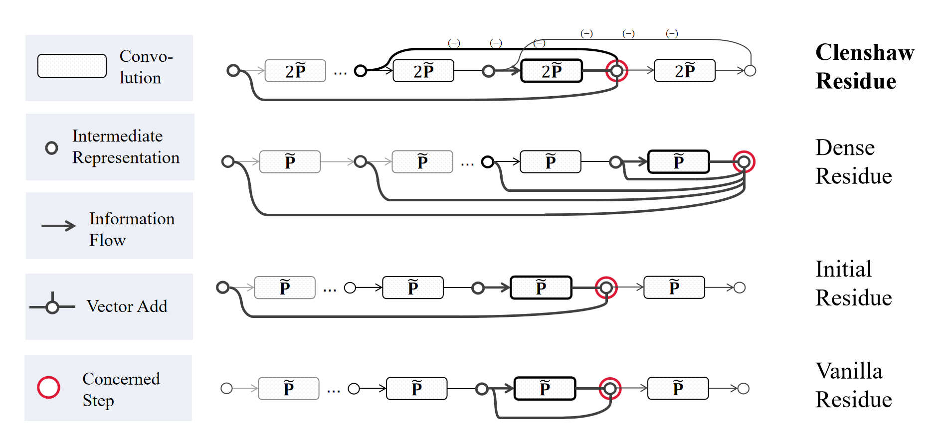
Figure 1. Illustration of different graph residual connections. Raw Residue and Initial Residue follows a single-line structure, Dense Residue connect densely to all the former layers, while our Clenshaw Residue achieves strong expressive power by a neat double-line structure.

figure description

Following ResNet (He et al., 2016), various GNN models use different residual connection techniques to overcome the problem of model degradation. As shown in Figure 1, we broadly classify the graph residual connections into three types:

• Raw Residual Connections are directly transplanted to GCNs in early attempts (Kipf and Welling, 2017), but they lose effectiveness when models come deeper(Xu et al., 2018; Chen et al., 2020). The reason behind this was gradually clarified with the discussion of over-smoothing (Li et al., 2018; Rong et al., 2020) .

• Initial Residual Connections (Klicpera et al., 2019a; Chen et al., 2020) are intuited by personalized pagerank, following the perspective of viewing GCNs with raw residues as lazy random walk (Xu et al., 2018; Wang et al., 2019), which converges to the stationary vector. Equipped with initial residues, the final representation implicitly leverages features of all fused levels. However, despite its ability to eliminate over-smoothing, models with initial residual connections in fact employees the homophily assumption (McPherson et al., 2001), that is, the assumption that connected nodes tend to share similar features and labels, which might be unsuitable for heterophilic graphs (Pei et al., 2020; Zheng et al., 2022). Some variants are also explored (Liu et al., 2021; Zhang et al., 2022), but they still fall into the scope of homophily.

• There are also Dense Residual Connections, which believe that, by exhibiting feature maps after different times of convolutions and combining them selectively, it is helpful for making extensive use of multi-scale information (Abu-El-Haija et al., 2019; Xu et al., 2018). The connection pattern in DenseNet (Iandola et al., 2014) is also exploited in  (Li et al., 2019), where they connect each layer to all former layers, incurs unaffordable space consumption.

Residual Connections and Polynomial Filters

On the other hand, the idea of making extensive use of multi-scale representations is closely related to Spectral Graph Neural Networks, which motivates us to inject the characteristics of spectral GNNs into our model by residual connections. Spectral GNNs gain their power from utilizing atomic structural components decomposed from the underlying graph. Spectral GNNs project features onto these components, and modulate the importance of the components by a filter. When this filter is a $K$-order polynomial function on the graph’s Laplacian spectrum, explicit decompositions of matrices are avoided, replaced by additions and subtractions of localized propagation results within different neighborhood radii, building a connection with ‘residual connection’.

Often, the problem of polynomial filtering is reduced to learning a proper polynomial function in order $K$. The expressive power in terms of representing arbitrary polynomial filters has been discussed in former graph residual connection works, especially dense residues (Abu-El-Haija et al., 2019; Chien et al., 2021). However, motivated from the spatial view of message passing, these works lose an important part of spectral graph learning: the employee of polynomial bases. Polynomial bases are of considerable significance when learning filtering functions. Until now, different polynomial bases are utilized, including Chebyshev Basis (Defferrard et al., 2016; He et al., 2022), Bernstein Basis (He et al., 2021) etc. See the example of Runge Phenomenon in (He et al., 2022) for an illustration of its importance.

Contributions

This paper focuses on the design of graph residual connections that exploit the expressive power of spectral polynomial filters. As we have demonstrated, raw residual connections and initial residual connections are primarily concerned with mitigating over-smoothing, and they commonly rely on the homophily assumption. Some dense residual connections do increase the expressive capacity of a GNN, with analyses aligning the spatial process with a potentially arbitrary spectral polynomial filter. Unfortunately, these works do not take the significance of different polynomial bases into account and are therefore incapable of learning a more effective spectral node representation.

In this paper, we introduce ClenshawGCN, a GNN model that employs the Clenshaw Summation Algorithm to enhance the expressiveness of the GCN model. More specifically, we list our contributions as follows:

• Powerful residual connection submodules. We propose ClenshawGCN, a message-passing GNN which borrows spectral power by adding two simple residual connection modules to each convolution layer: an adaptive initial residue and a negative second order residue;

• Expressive power in terms of polynomial filters We show that a $K$-order ClenshawGCN simulates any $K$-order polynomial function based on the Chebyshev basis of the Second Kind. More specifically, the adaptive initial residue allows for the flexibility of coefficients, while the negative second order residue allows for the implicit use of Chebyshev basis. We prove this by the Clenshaw Summation Algorithm for Chebyshev basis (the Second Kind).

• Outstanding performances. We compare ClenshawGCN with both spatial and spectral models. Extensive empirical studies demonstrate that ClenshawGCN outperforms both spatial and spectral models on various datasets.

2. Preliminaries

2.1. Notations

We consider a simple graph $\mathcal{G}=(\mathcal{V},\mathcal{E},\mathbf{A})$, where $\mathcal{V}=\{1,2,\cdots,n\}$ is a finite node-set with $|\mathcal{V}|=n$, $\mathcal{E}$ is an edge-set with $|\mathcal{E}|=m$, and $\mathbf{A}$ is an unnormalized adjacency matrix. $\mathcal{L}=\mathbf{D}-\mathbf{A}$ denotes $\mathcal{G}^{\prime}s$ unnormalized graph Laplacian, where $\mathbf{D}=\text{diag}\{d_{1},\cdots,d_{n}\}$ is the degree matrix with $d_{i}=\sum_{j}{\mathbf{A}_{ij}}$.

Following GCN, we add a self-connecting edge is to each node, and conduct symmetric normalization on $\mathcal{L}$ and $\mathbf{A}$. The resulted self-looped symmetric-normalized adjacency matrix and Laplacian are denoted as $\tilde{\mathbf{P}}=(\mathbf{D}+\mathbf{I})^{-1/2}(\mathbf{A}+\mathbf{I})(\mathbf{D}+\mathbf{I})^{-1/2}$ and $\tilde{\mathcal{L}}=\mathbf{I}-\tilde{\mathbf{P}}$, respectively.

Further, we attach each node with an $f$-dimensional raw feature and denote the feature matrix as $\mathbf{X}\in\mathbb{R}^{n\times f}$. Based on the the topology of underlying graph, GNNs enhance the raw node features to better representations for downstream tasks, such as node classification or link prediction.

2.2. Spatial Background

Layer-wise Message Passing Architecture

From a spatial view, the main body of a Graph Neural Network is a stack of convolution layers, who broadcast and aggregate feature information along the edges. Such a graph neural network is also called a Message Passing Neural Network (MPNN). To be concrete, we consider an MPNN with $K$ graph convolution layers and denote the nodes’ representations of the $\ell$-th layer as $\mathbf{H}^{(\ell)}$. $\mathbf{H}^{(\ell)}$ is constructed based on $\mathbf{H}^{(\ell-1)}$ by an propagation and possibly a transformation operation. For example, in Vanilla GCN (Kipf and Welling, 2017), the convolution layer is defined as

(1) $$\mathbf{H}^{(\ell)}=\sigma(\tilde{\mathbf{P}}\mathbf{H}^{(\ell-1)}\mathbf{W}^{(\ell)})),$$

whose $propagation$ operator is $\displaystyle f:{\mathbf{H}}^{(\ell-1)}\to\tilde{\mathbf{P}}\mathbf{H}^{(\ell-1)}$ and transformation operator is $\displaystyle f:\tilde{\mathbf{P}}\mathbf{H}^{(\ell-1)}\to\sigma(\tilde{\mathbf{P}}\mathbf{H}^{(\ell-1)}\mathbf{W}^{(\ell)}))$.

Extra transformations, or probably combinations, are applied before and after the stack of $K$ convolution layers to form a map from $\mathbf{X}$ to the final output $\hat{\mathbf{Y}}$, which is determined by the downstream task, e.g. $\mathbf{H}^{(0)}=\text{MLP}(\mathbf{X};\mathbf{W}^{(0)})$ and $\hat{\mathbf{Y}}=\text{SoftMax}(\text{MLP}(\mathbf{H}^{(K)};\mathbf{W}^{(K+1)}))$ for node classification tasks. In this paper, a slight difference in notation lies in that, we denote the input of convolution layers to be $\mathbf{H}^{*}$, instead of $\mathbf{H}^{(0)}$, and introduce notations $\mathbf{H}^{(-1)}$ and $\mathbf{H}^{(-2)}$ as zero matrices for simplicity of later representation.

Entangled and Disentangled Architectures

The motivations for propagation and transformation in a convolution layer differ. Propagations are related to graph topology, analyzed as an analog of walks (Xu et al., 2018; Wang et al., 2019; Klicpera et al., 2019a; Chen et al., 2020), diffusion processes (Zhao et al., 2021; Klicpera et al., 2019b; Chamberlain et al., 2021), etc. , while the entangling of transformations between propagations follows behind the convention of deep learning. A GNN is classified under a disentangled architecture if the transformations are disentangled from propagations, such as APPNP (Klicpera et al., 2019a) and GPRGNN (Chien et al., 2021). Though it is raised in  (Zhang et al., 2022) that the entangled architecture tends to cause model degradations, we observe that GCNII (Chen et al., 2020) under the entangled architecture does not suffer from this problem. So we follow the use of entangled transformations as in Vanilla GCN, and leverage the identity mapping of weight matrices as in GCNII.

2.3. Spectral Background

Spectral Definition of Convolution

Graph spectral domain leverages the geometric structure of underlying graphs in another way (Shuman et al., 2013).

Conduct eigen-decomposition on $\tilde{\mathcal{L}}$, i.e. $\tilde{\mathcal{L}}=\mathbf{U}\mathbf{\Lambda}\mathbf{U}^{T}$, the spectrum $\mathbf{\Lambda}$ $=\text{diag}\{\lambda_{1},\cdots,\lambda_{n}\}$ is in non-decreasing order. Since $\tilde{\mathcal{L}}$ is real-symmetric, elements in $\mathbf{\Lambda}$ are real, and $\mathbf{U}$ is a complete set of $n$ orthonormal eigenvectors, which is used as a basis of frequency components analogously to classic Fourier transform .

Now consider a column in $\mathbf{X}$ as a graph signal scattered on $\mathcal{V}$, denoted as $\mathbf{x}\in\mathbb{R}^{n}$. Graph Fourier transform is defined as $\displaystyle\hat{\mathbf{x}}:=\langle\mathbf{U},\mathbf{x}\rangle=\mathbf{U^{T}x}$, which projects graph signal $\mathbf{x}$ to the frequency responses of basis components $\hat{\mathbf{x}}$. It is then followed by modulation, which can be presented as $\displaystyle\mathbf{\hat{x}}^{*}:=g_{\mathbf{\theta}}\mathbf{\hat{x}}=\text{diag}\{\theta_{1},\cdots\theta_{n}\}\mathbf{\hat{x}}$. After modulation, inverse Fourier transform: $\displaystyle\mathbf{x}^{*}:=\mathbf{U}\mathbf{{\hat{x}}^{*}}$ transform $\mathbf{{\hat{x}}^{*}}$ back to the spatial domain. The three operations form a spectral definition of convolution:

(2) $$g_{\theta}\star\mathbf{x}=\mathbf{U}g_{\theta}\mathbf{U}^{T}\mathbf{x},$$

which is also called spectral filtering. Specifically, when $\theta_{i}=1-\lambda_{i}$, $\mathbf{U}g_{\theta}\mathbf{U}^{T}\mathbf{x}\equiv\tilde{\mathbf{P}}\mathbf{x}$, giving an spectral explanation of GCN’s convolution in Equation (1).

Polynomial Filtering

The calculation of $\mathbf{U}$ in Equation (2) is of prohibitively expensive. To avoid explict eigen-decomposition of ${\mathbf{U}}$, $g_{\theta}$ is often defined as a polynomial function of a frequency component’s corresponding eigenvalue parameterized by $\theta$, that is,

$$\mathbf{{\hat{x}}^{*}}_{i}=g_{\theta}(\lambda_{i})\langle\mathbf{U}_{i},\mathbf{x}\rangle.$$

The spectral filtering process then becomes

(3) $$g_{\theta}\star\mathbf{x}=\mathbf{U}g_{\theta}(\mathbf{\Lambda})\mathbf{U}^{T}\mathbf{x}\equiv g_{\theta}(\tilde{\mathcal{L}})\mathbf{x},$$

where $g_{\theta}(\tilde{\mathcal{L}})\mathbf{x}$ elimates eigen-decomposition and can be calculated in a localized way in $\mathcal{O}(|\mathcal{E}|)$  (Defferrard et al., 2016; Kipf and Welling, 2017).

Equivalently, we can define the filtering function on the spectrum of $\mathbf{\tilde{P}}$, instead of $\tilde{\mathcal{L}}$. Since $\mathbf{\tilde{P}}=\mathbf{I}-\tilde{\mathcal{L}}$, $\mathbf{\tilde{P}}$ and $\tilde{\mathcal{L}}$ share the same set of orthonormal eigenvectors $\mathbf{U}$, and the spectrum of $\mathbf{\tilde{P}}$, denoted as $\mathbf{M}=\{\mu_{1},\cdots,\mu_{n}\}$, satisfies $\mu_{i}=1-\lambda_{i}(i=1,\cdots,n)$ . Thus, the filtering function can be defined as $h_{\theta}$, where

(4) $$\hbox{\pagecolor{gray!15}$\displaystyle h_{\theta}(\mu)\equiv g_{\theta}(1-\mu)$}.$$

In Section 3, for the brevity of presentation, we will use this equivalent definition.

2.4. Polynomial Approximation and Chebyshev Polynomials

Polynomial Approximation

Following the idea of polynomial filtering (Equation (3)), the problem then becomes the approximation of polynomial $g_{\theta}$. A line of work approximates $g_{\theta}$ by some truncated polynomial basis $\{\phi_{i}(x)\}_{i=0}^{i=K}$ up to the $K$-th order, i.e.

$$g_{\theta}(x)=\sum_{k=0}^{K}\theta_{i}\phi_{i}(x),$$

where $\vec{\theta}=\left[\theta_{0},\cdots,\theta_{K}\right]\in\mathbb{R}^{K+1}$ is the coefficients. In the field of polynomial filtering and spectral GNNs, different bases have been explored for $\{\phi_{i}(x)\}_{i=0}^{i=K}$, including Chebyshev basis (Defferrard et al., 2016), Bernstein basis (He et al., 2021), Jacobi basis (Wang and Zhang, 2022), etc.

Chebyshev Polynomials

Chebyshev basis has been explored since early attempts for the approximation of $g_{\theta}$ (Defferrard et al., 2016). Besides Chebyshev polynomials of the first kind ( $\{T_{i}(x)\}_{i=0}^{\infty}$ ), the second kind ( $\{U_{i}(x)\}_{i=0}^{\infty}$ ) is also wildly used.

Both $\{T_{i}(x)\}_{i=0}^{\infty}$ and $\{U_{i}(x)\}_{i=0}^{\infty}$ can be generated by a recurrence relation:

$$T_{0}(x)=1,\quad T_{1}(x)=x,$$

$$T_{n}(x)=2xT_{n-1}(x)-T_{n-2}(x).\quad(n=2,3,\cdots)$$

$$U_{-1}(x)=0,\quad U_{0}(x)=1,U_{1}(x)=2x,$$

(5) $$U_{n}(x)=2xU_{n-1}(x)-U_{n-2}(x).\quad(n=1,2,\cdots)$$

The recurrence relation is used in ChebyNet (Defferrard et al., 2016) for accelarating the computing of polynomial filtering. Note that we start the second kind from $U_{-1}$, which will be used in later proof in Section 3.3.

2.5. Residual Network Structures

We have discussed some graph residual connections in Introduction . In this section, we list some model in detail for illustration of residual connections.

GCNII equips the vanilla GCN convolution with two techniques: initial residue and identity mapping:

(6) $$\mathbf{H}^{(\ell)}=\sigma\left(\left((1-\alpha)\tilde{\mathbf{P}}\mathbf{H}^{(\ell-1)}+\alpha\mathbf{H}^{*}\right)\left((1-\beta_{\ell})\mathbf{I}_{n}+\beta_{\ell}\mathbf{W}^{(\ell)}\right)\right).$$

Ignoring non-linear transformation, GCNII iteratively solves the optimization problem:

(7) $$\underset{\mathbf{H}}{\arg\min}\quad{\alpha}\left\|\mathbf{H}-\mathbf{H}^{*}\right\|_{F}^{2}+(1-\alpha)\operatorname{tr}\left(\mathbf{H}^{\top}\tilde{\mathcal{L}}\mathbf{H}\right).$$

The optimization goal reveals the underlying homophily assumption, where initial residual connection is only making a compromise between Laplacian smoothing and keeping identity.

AirGNN (Liu et al., 2021) proposes an extension for initial residue, where the first term of optimization problem in Equation (7) is replaced by the $\ell_{21}$ norm. By solving the optimization problem, AirGNN adaptively choose $\alpha$. However, limited by the optimization goal, AirGNN still falls into the homophility assumption.

JKNet (Xu et al., 2018) uses dense residual connection at the last layer and combine all the intermediate representations nodewisely by different ways, including LSTM, Max-Pooling and so on.

MixHop (Abu-El-Haija et al., 2019) concats feature maps of several hops at each layer, represented as

$$\mathbf{H}^{(\ell+1)}=\underset{j\in K}{\Bigg{\|}}\sigma\left(\tilde{\mathbf{P}}^{j}\mathbf{H}^{(\ell)}\mathbf{W}_{j}^{(\ell)}\right),$$

which can be considered as staking several dense graph residual networks.

3. Method

3.1. Clenshaw Convolution

We formulate the $\ell$-th layer’s representation of ClenshawGCN as

(8) $$\mathbf{H}^{(\ell)}=\sigma\left(\left(2\mathbf{\tilde{P}}\mathbf{H}^{(\ell-1)}\hbox{\pagecolor{gray!15}$\displaystyle-\mathbf{H}^{(\ell-2)}$}+\hbox{\pagecolor{gray!15}$\displaystyle\alpha_{\ell}\mathbf{H}^{*}$}\right)\left((1-\beta_{\ell})\mathbf{I}_{n}+\beta_{\ell}\mathbf{W}^{(\ell)}\right)\right),$$

where $\ell=0,1,\ldots,K$, $\mathbf{H}^{(-2)}=\mathbf{H}^{(-1)}=\mathbf{O}$, $\mathbf{H}^{*}=\text{MLP}(\mathbf{X};\mathbf{W^{*}})$.

Note that for transformation, we use identity mapping with $\beta_{\ell}=\log(\frac{\lambda}{\ell}+1)\approx\lambda/\ell$ following GCNII (Chen et al., 2020). Comparing to GCNII, we include two simple yet effective residual connections: Adaptive Initial Residue and Negative Second Order Residue:

$$2\mathbf{\tilde{P}}\mathbf{H}^{(\ell-1)}\underbrace{\hbox{\pagecolor{gray!15}$\displaystyle-\mathbf{H}^{(\ell-2)}$}}_{\begin{subarray}{c}\text{ {Negative} \text@underline{Second}}\\ \text{\text@underline{Order} Residue}\end{subarray}}+\underbrace{\hbox{\pagecolor{gray!15}$\displaystyle\alpha_{\ell}\mathbf{H}^{*}$}.}_{\begin{subarray}{c}\text{{Adaptive}}\\ \text{\text@underline{Initial} Residue}\end{subarray}}$$

In the remaining part of this section, we will illustrate the role and mechanism of these two residual modules. In summary, adaptive initial residue enables the simulating of any $K$-order polynomial filter, while negative second order residue, motivated by the leveraging of ‘differencing relations’, simulates the use of Chebyshev basis in the approximation of filtering functions. For both two parts, we will give an intuitive analysis with followed by a proofs.

3.2. Adaptive Initial Residue

The role of adaptive initial residue is to enable the expressive power of any $K$-order polynomial filter. To illustrate this, we will first consider an incomplete version of the ClenshawGCN termed HornerGCN.

Intuition

We start with an analysis of GCNII. To simplify the analysis, we consider $(1-\beta_{\ell})\mathbf{I}_{n}+\beta_{\ell}\mathbf{W}^{(\ell)}$ as $\mathbf{I}$, and take $\textrm{relu}(x)=x$. At this point, the iteration (6) is simplified as

(9) $$\mathbf{H}^{(\ell)}=(1-\alpha)\tilde{\mathbf{P}}\mathbf{H}^{(\ell-1)}+\alpha\mathbf{H}^{*}.$$

Consider a GCNII model of order $K$, by expanding (9), we obtain that

(10) $$\mathbf{H}^{(K)}=\sum_{\ell=0}^{K}\hat{\alpha}_{\ell}\tilde{\mathbf{P}}^{\ell}\mathbf{H}^{*},$$

where

$$\hat{\alpha}_{\ell}=\left\{\begin{matrix}\alpha(1-\alpha)^{\ell},&\ell<K,\\ (1-\alpha)^{K},&\ell=K.\end{matrix}\right.$$

It can be seen that the iterative process of GCNII implicitly leverages the representations of different layers with fixed and positive coefficients. However, we want flexible exploitation of different diffusion layers, (Xu et al., 2018; Zhao et al., 2021). More importantly, we need to have negative weights in cases of heterophilic graphs (Chien et al., 2021). To this end, we can simply replace the fixed $\alpha$ in (6) with learnable ones. In this way, we obtain the form of HornerGCN as follows,

(11) $$\mathbf{H}^{(\ell)}=\sigma\left(\left(\mathbf{\tilde{P}}\mathbf{H}^{(\ell-1)}+\hbox{\pagecolor{gray!15}$\displaystyle\alpha_{\ell}\mathbf{H}^{*}$}\right)\left((1-\beta_{\ell})\mathbf{I}_{n}+\beta_{\ell}\mathbf{W}^{(\ell)}\right)\right),$$

where $\ell=0,1,\ldots,K$, $\mathbf{H}^{(-1)}=\mathbf{O}$, $\mathbf{H}^{*}=\text{MLP}(\mathbf{X};\mathbf{W^{*}})$.

Spectral Nature

With the definition of polynomial filters given in Equation (4) and Definition 2.1, we will prove the Theorem below:

Horner’s Method

To prove Theorem 3.1, we first briefly introduce Horner’s Method (Horner, 1819). Given $p(x)=\sum_{i=0}^{n}a_{i}x^{i}=a_{0}+a_{1}x+\cdots a_{n}x^{n}$, Horner’s Method is a classic method for evaluating $p(x_{0})$, by viewing $p(x)$ as the following form:

(12) $$p(x)=a_{0}+x\left(a_{1}+x\left(a_{2}+x\left(a_{3}+\cdots+x\left(a_{n-1}+xa_{n}\right)\cdots\right)\right)\right).$$

Thus, Horner’s method defines a recursive method for evaluating $p(x_{0})$:

$$b_{n} :=a_{n},$$

$$b_{n-1} :=a_{n-1}+b_{n}x_{0},$$

$$\cdots$$

$$b_{0} :=a_{0}+b_{1}x_{0},$$

(13) $$p(x_{0}) :=b_{0}.$$

Proof of Spectral Expressiveness

Note that the form of Horner’s recursive are parallel with the recursive of stacked Horner convolutions by ignoring the non-linear transformations. Thus, by unfolding the nested expression of Horner convolutions (11), we get the output of the last layer closely matched with the form of Equation (12) :

So, the final representation

$$\mathbf{H}^{(K)} =\sum_{\ell=0}^{K}\alpha_{K-\ell}\tilde{\mathbf{P}}^{\ell}\mathbf{H}^{*}=\mathbf{U}\left(\sum_{\ell=0}^{K}{\alpha}_{K-\ell}\mathbf{M}^{\ell}\right)\mathbf{U}^{T}\mathbf{H}^{*},$$

corresponds to the result of a polynomial filter $h$ on the spectrum of $\mathbf{\tilde{P}}$, where

$$h(\mu)=\sum_{\ell=0}^{K}{\alpha}_{K-\ell}\mu^{\ell}.$$

3.3. Negative Second Order Residue

The role of negative second order residue is to enable the leverage of Chebyshev basis. Compared with the adaptive initial residue, it is not obvious. In this section, we will first give an intuitive motivation for Negative Second Order Residue, and then reveal the mechanism behind it by Clenshaw Summation Algorithm.

Intuition of Taking Difference

There is already some work that has noticed the ‘subtraction’ relationship between progressive levels of representation (Abu-El-Haija et al., 2019; Yang et al., 2022). For example, one of MixHop’s direct challenges towards the traditional GCN model is the inability to represent the Delta Operator, i.e., $\mathbf{AX}^{2}{\color[rgb]{1,0,0}-}\mathbf{AX}$, which is an important relationship in representing both the concept of social boundaries (Perozzi and Akoglu, 2018) and the concept of ‘sharpening’ in images (Burt and Adelson, 1987; Paris et al., 2011).

Instead of considering model’s ability to represent Delta Operator in the final output, we take a more direct use of these difference relations. That is, we add $\displaystyle\mathbf{\tilde{P}}\mathbf{H}^{(\ell-1)}-\mathbf{H}^{(\ell-2)}$ to each convolution layers of (11), and get the final form of Clenshaw Convolution:

$$\mathbf{\tilde{P}}\mathbf{H}^{(\ell-1)}+\alpha_{\ell}\mathbf{H}^{*}+\hbox{\pagecolor{gray!15}$\displaystyle\mathbf{\tilde{P}}\mathbf{H}^{(\ell-1)}-\mathbf{H}^{(\ell-2)}$}\Longrightarrow\eqref{eq:clenshaw_conv}.$$

A question that perhaps needs to be answered is: why not instead insert a more direct difference relation: $\underline{\mathbf{\tilde{P}}\mathbf{H}^{(\ell-1)}-\mathbf{H}^{(\ell-1)}}$ ? The reason is, at this point, the convolution would become

$$\mathbf{\tilde{P}}\mathbf{H}^{(\ell-1)}+\alpha_{\ell}\mathbf{H}^{*}+\underline{\mathbf{\tilde{P}}\mathbf{H}^{(\ell-1)}-\mathbf{H}^{(\ell-1)}}=\left(2\mathbf{\tilde{P}}-\mathbf{I}\right)\mathbf{H}^{(\ell-1)}+\alpha_{\ell}\mathbf{H}^{*},$$

whose unfolded form, by substitute $\mathbf{\tilde{P}}$ to $2\mathbf{\tilde{P}}-\mathbf{I}$ in (3.2), would become $\sum_{\ell=0}^{K}\alpha_{K-\ell}{\left(2\tilde{\mathbf{P}}-\mathbf{I}\right)}^{\ell}\mathbf{H}^{*}$ , which brings limited change.

Spectral Nature

Besides the spatial intuition of considering substractions or boundaries, we reveal the spectral nature of our negative residual connection in this part, that is, it simulates the leverage of chebyshev basis as in spectral polynomials. With the definition of polynomial filters given in Equation (4) and Definition 2.1, we will prove the theorem below:

which can also be expressed as:

(15) $$\mathbf{H}^{(K)}=\mathbf{U}h({\mathbf{M}})\mathbf{U}^{T}\mathbf{H}^{*}=\mathbf{U}\left(\sum_{\ell=0}^{K}{\alpha}_{K-\ell}U_{\ell}(\mathbf{M})\right)\mathbf{U}^{T}\mathbf{H}^{*}.$$

Clenshaw Algorithm

For the proof of Theorem 3.2, we will first introduce Clenshaw Summation Algorithm as a Corollary.

Clenshaw Summation can be applied to a wider range of polynomial basis. However, specifically for the second kind of Chebyshev, we made some slight simplifications, so for clarity of discussion, we give the proof here.

Proof for Corollary 3.3.

Denote

$$A=\begin{bmatrix}1&&&&\\ -2x&1&&&\\ 1&-2x&1&&\\ &&\cdots&&\\ &&1&-2x&1\end{bmatrix},\quad\vec{u}=\begin{bmatrix}U_{-1}(x)\\ U_{0}(x)\\ U_{1}(x)\\ \cdots\\ U_{n}(x)\end{bmatrix},\quad\vec{a}=\begin{bmatrix}0\\ a_{0}\\ a_{1}\\ \cdots\\ a_{n}\end{bmatrix},$$

with $A\in\mathbb{R}^{(n+2)\times(n+2)}$, $\vec{u}\in\mathbb{R}^{n+2}$, then

(17) $$S(x)=\vec{a}^{T}\vec{u}.$$

Indexing a vector from $-1$, we denote $\mathbf{1}_{i}\in\mathbb{R}^{(n+2)}$ as the one-hot vector with the $i$-th element being $1$ ($i$ starts from $-1$). Note that, since the recurrence relation for the Chebyshev polynomials (2.4),

(18) $$A\vec{u}=\begin{bmatrix}U_{-1}(x)\\ -2xU_{-1}(x)+U_{0}(x)\\ 0\\ \cdots\\ 0\end{bmatrix}=\begin{bmatrix}0\\ U_{0}(x)\\ 0\\ \cdots\\ 0\end{bmatrix}=\mathbf{1}_{0}.$$

Now suppose that there is a vector $\vec{b}=[b_{-1},b_{0},\cdots,b_{n}]$ satisfying

(19) $$\vec{a}^{T}=\vec{b}^{T}A,$$

then

$$S(x)\stackrel{{\scriptstyle\eqref{eq:s}}}{{=}}\vec{a}^{T}\vec{u}\stackrel{{\scriptstyle\eqref{eq:suppose_b}}}{{=}}\vec{b}^{T}A\vec{u}\stackrel{{\scriptstyle\eqref{eq:cheb2-3-term}}}{{=}}\vec{b}\mathbf{1}_{0}=b_{0}.$$

On the other hand, notice that the recurrence defined in (3.3) is exactly the Gaussian Elimination process of solving $\vec{a}^{T}=\vec{b}^{T}A$ from $b_{n}$ down to $b_{0}$, which means that $\{b_{n},\cdots,b_{0}\}$ calculated by (3.3) satisfies (19). Proof for Corollary 3.3 is finished. ∎

Proof of Spectral Expressiveness

Now we prove Theorem 3.2 inductively based on Corollary 3.3.

Proof of Theorem 3.2.

Given:

(20) $$\mathbf{H}^{(\ell)}=2\mathbf{\tilde{P}}\mathbf{H}^{(\ell-1)}{-\mathbf{H}^{(\ell-2)}}+{\alpha_{\ell}\mathbf{H}^{*}},$$

$\mathbf{H}^{(-1)}=\mathbf{H}^{(-2)}=\mathbf{0}$.

Induction Hypothesis: Suppose that when the convolutions have processed to the $\ell$-th layer, $\mathbf{H}^{(\ell-1)}$ and $\mathbf{H}^{(\ell-2)}$ are already proved to be polynomial filtered results of $\mathbf{H}^{*}$, we show that $\mathbf{H}^{(\ell)}$ is also polynomial filtered results of $\mathbf{H}^{*}$.

Further, denote the polynomial filtering functions of generating $\mathbf{H}^{(\ell-2)}$, $\mathbf{H}^{(\ell-1)}$ and $\mathbf{H}^{(\ell)}$ to be $h^{(\ell-2)}$, $h^{(\ell-1)}$ and $h^{(\ell)}$. Then $h^{(\ell)}$ satisfies:

$$h^{(\ell)}(\mu) =\alpha_{\ell}+2\mu h^{(\ell-1)}(\mu)-h^{(\ell-2)}(\mu).$$

Base Case: For $\ell=0$, since $\mathbf{H}^{(-2)}=\mathbf{H}^{(-1)}=\mathbf{0}$, $\mathbf{H}^{(0)}=\alpha_{0}\mathbf{H}^{*}$, the first induction step is established with

$$h^{(0)}(\mu)=\alpha_{0},\quad h^{(-1)}(\mu)=0,\quad h^{(-2)}(\mu)=0.$$

Induction Step: Insert

$$\left\{\begin{matrix}\mathbf{H}^{(\ell-1)}&=\mathbf{U}h^{\ell-1}(\mathbf{M})\mathbf{U}^{T}\mathbf{H}^{*},\\ \mathbf{H}^{(\ell-2)}&=\mathbf{U}h^{\ell-2}(\mathbf{M})\mathbf{U}^{T}\mathbf{H}^{*},\\ \mathbf{\tilde{P}}&=\mathbf{U}\mathbf{M}\mathbf{U}^{T}\end{matrix}\right.$$

into Equation (20), we get

$$\mathbf{H}^{(\ell)} =2\underline{\mathbf{U}\mathbf{M}\mathbf{U}^{T}}\dashuline{\mathbf{U}h^{(\ell-1)}(\mathbf{M})\mathbf{U}^{T}\mathbf{H}^{*}}-\dashuline{\mathbf{U}h^{(\ell-2)}(\mathbf{M})\mathbf{U}^{T}\mathbf{H}^{*}}+{\alpha_{\ell}\mathbf{H}^{*}}$$

$$=\mathbf{U}\left(\alpha_{\ell}+2\mathbf{M}h^{(\ell-1)}(\mathbf{M})-h^{(\ell-2)}(\mathbf{M})\right)\mathbf{U}^{T}\mathbf{H}^{*}.$$

So, $\mathbf{H}^{(\ell)}$ is also a polynomial filtered result of $\mathbf{H}^{*}$, with filtering function $h^{(\ell)}$:

(21) $$h^{(\ell)}(\mu):=\alpha_{\ell}+2\mu h^{(\ell-1)}(\mu)-h^{(\ell-2)}(\mu).$$

Stack relation(21) for $\ell=0,1,\cdots,K$, we get:

$$h^{(-2)}(\mu) =0,$$

$$h^{(-1)}(\mu) =0,$$

$$h^{(\ell)}(\mu) :=\alpha_{\ell}+2\mu h^{(\ell-1)}(\mu)-h^{(\ell-2)}(\mu),\quad$$

$$\quad\quad(k=0,1,\cdots,K).$$

where the progressive access of $b^{(\ell)}$ is in a totally parallel way with the recurrence (3.3) in Clenshaw Summation Algorithm. We soonly get

$$\sum_{\ell=0}^{K}{\alpha}_{K-\ell}U_{\ell}(\mu)\equiv h^{(K)}(\mu).$$

Thus, we have finshed the proof of Theorem 3.2 . ∎

4. Experiments

In this section, we conduct two sets of experiments with the node classification task. First, we verify the power of our method by comparing it with both spatial residual methods and powerful spectral models. Second, we verify the effectiveness of the two submodules by ablation studies.

4.1. Experimental Setup

Datasets and Splits

We use both homophilic graphs and heterophilic graphs in our experiments following former works, especially GCN (Kipf and Welling, 2017), Geom-GCN (Pei et al., 2020) and LINKX (Lim et al., 2021).

• Citation Graphs. Cora, PubMed, and CiteSeer are citation datasets (Sen et al., 2008) processed by Planetoid (Yang et al., 2016). In these graphs, nodes are scientific publications, edges are citation links processed to be bidirectional, and node features are bag-of-words representations of the documents. These graphs show strong homophily.

• Wikipedia Graphs. Chameleon dataset and Squirrel dataset are page-page networks on topics in Wikipedia, where nodes are entries, and edges are mutual links.

• Webpage Graphs. Texas dataset and Cornell dataset collect web pages from computer science departments of different universities. The nodes in the graphs are web pages of students, projects, courses, staff or faculties (Craven et al., 1998), the edges are hyperlinks between them, and node features are the bag-of-words representations of these web pages.

• Co-occurrence Network. The Actor network represents the co-occurrence of actors on a Wikipedia page (Tang et al., 2009). The node features are filtered keywords in the Wikipedia pages. The categorization of the nodes is done by (Pei et al., 2020).

• Mutual follower Network. Twitch-Gamers dataset represents the mutual following relationship between accounts on the streaming platform Twitch.

We list the messages of these networks in Table 1, where $\mathcal{H}(G)$ is the measure of homophily in a graph proposed by Geom-GCN (Pei et al., 2020). Larger $\mathcal{H}(G)$ implies stronger homophily.

Table 1. Statistics for the node classification datasets we use. Datasets of different homophily degrees are used.

Dataset	#Nodes	#Edges	#Classes	$\mathcal{H}(G)$
Cora	2,709	5,429	7	.83
Pubmed	19,717	44,338	3	.71
Citeseer	3,327	4,732	6	.79
Squirrel	5,201	217,073	5	.22
Chameleon	7,600	33,544	5	.23
Texas	183	309	5	.11
Cornell	183	295	5	.30
Twitch-Gamers	168,114	6,797,557	7	.55

For all datasets except for the Twitch-gamers dataset, we take a 60%/20%/20% train/validation/test split proportion following former works (Pei et al., 2020; Chien et al., 2021; He et al., 2021, 2022). We run these datasets twenty times over random splits with random initialization seeds. For the Twitch-gamers dataset, we use the five random splits given in LINKX (Lim et al., 2021) with a 50%/25%/25% proportion to align with reported results.

ClenshawGCN Setup

Before and after the stack of Clenshaw convolution layers, two non-linear transformations are made to link with the dimensions of the raw features and final class numbers. All the intermediate transformation layers are set with 64 hidden units. For the initialization of the adaptive initial residues’ coefficients, denoted as $\vec{\alpha}=\left[\alpha_{0},\cdots,\alpha_{K}\right]$, we simply set ${\alpha_{K}}$ to be $1$ and all the other coefficients to be $0$, which corresponds to initializing the polynomial filter to be $\displaystyle g(\lambda)=1$ (or equivalently, $\displaystyle h(\mu)=1$ ).

Hyperparameter Tuning

For the optimization process on the training sets, we tune $\vec{\alpha}$ with SGD optimizer with momentum (Sutskever et al., 2013) and all the other parameters with Adam SGD (Kingma and Ba, 2014). We use early stopping with a patience of 300 epochs.

For the search space of hyperparameters, below is the search space of hyperparameters:

• Orders of convolutions: $K\in\left\{8,12,\cdots,32\right\}$;

• Learning rates: $\left\{0.001,0.005,0.1,0.2,0.3,0.4,0.5\right\}$;

• Weight decays: $\left\{1\mathrm{e}{-8},1\mathrm{e}{-7},\cdots,1\mathrm{e}{-3}\right\}$;

• Dropout rates: $\left\{0,0.1,\cdots,0.7\right\}$.

We tune all the hyperparameters on the validation sets. To accelerate hyperparameter searching, we use Optuna (Akiba et al., 2019) and run 100 completed trials for each dataset.

4.2. Comparing ClenshawGCN with Other Graph Residual Connections

Table 2. Comparison with other models equipped by different kinds of residual connections. Mean classification accuracies (± standard derivation) of random splits are displayed. Besides the ClenshawGCN, all the results are taken directly from (Luan et al., 2021) and (Lim et al., 2021). For the Twitch-Gamer dataset, we use 5 fixed 50%/25%/25% splits given in (Lim et al., 2021) to align with the reported results. For all the other datasets, 20 random 60%/20%/20% splits were used. (M) denotes some hyperparameter settings run out of memory (Lim et al., 2021).

Datasets	Chameleon	Squirrel	Actor	Texas	Cornell	Cora	Citeseer	Pubmed	Twitch-gamer
$|\mathcal{V}|$	2,277	5,201	7,600	183	183	2,708	3,327	19,717	168,114
MLP	46.59±1.84	31.01±1.18	40.18±0.55	86.81±2.24	84.15±3.05	76.89±0.97	76.52±0.89	86.14±0.25	60.92±0.07
GCN	60.81±2.95	45.87±0.88	33.26±1.15	76.97±3.97	65.78±4.16	87.18±1.12	79.85±0.78	86.79±0.31	62.18±0.26
GCNII	63.44±0.85	41.96±1.02	36.89±0.95	80.46±5.91	84.26±2.13	88.46±0.82	79.97±0.65	89.94±0.31	63.39±0.61
$\text{H}_{2}$GCN	52.30±0.48	30.39±1.22	38.85±1.17	85.90±3.53	86.23±4.71	87.52±0.61	79.97±0.69	87.78±0.28	(M)
MixHop	36.28±10.22	24.55±2.60	33.13±2.40	76.39±7.66	60.33±28.53	65.65±11.31	49.52±13.35	87.04±4.10	65.64±0.27
GCN+JK	64.68±2.85	53.40±1.90	32.72±2.62	80.66±1.91	66.56±13.82	86.90±1.51	73.77±1.85	90.09±0.68	63.45±0.22
ClenshawGCN	69.44±2.06	62.14±1.65	42.08±1.99	93.36±2.35	92.46±3.72	88.90±1.26	80.34±1.26	91.99±0.41	66.26±0.27

Table 3. Comparison with spectral models. Mean classification accuracies (±95% confidence intervals) on 20 random 60%/20%/20% train/validation/test splits are displayed. Besides the ClenshawGCN, all the results are taken directly from (He et al., 2021).

Datasets	Chameleon	Squirrel	Actor	Texas	Cornell	Cora	Citeseer	Pubmed
$|\mathcal{V}|$	2,277	5,201	7,600	183	183	2,708	3,327	19,717
ChebNet	59.51±1.25	40.81±0.42	37.42±0.58	86.28±2.62	83.91±2.17	87.32±0.92	79.33±0.57	87.82±0.24
ARMA	60.21±1.00	36.27±0.62	37.67±0.54	83.97±3.77	85.62±2.13	87.13±0.80	80.04±0.55	86.93±0.24
APPNP	52.15±1.79	35.71±0.78	39.76±0.49	90.64±1.70	91.52±1.81	88.16±0.74	80.47±0.73	88.13±0.33
GPRGNN	67.49±1.38	50.43±1.89	39.91±0.62	92.91±1.32	91.57±1.96	88.54±0.67	80.13±0.84	88.46±0.31
BernNet	68.53±1.68	51.39±0.92	41.71±1.12	92.62±1.37	92.13±1.64	88.51±0.92	80.08±0.75	88.51±0.39
ChebNetll	71.37±1.01	57.72±0.59	41.75±1.07	93.28±1.47	92.30±1.48	88.71±0.93	80.53±0.79	88.93±0.29
ClenshawGCN	69.44±0.92	62.14±0.70	42.08±0.86	93.36±0.99	92.46±1.64	88.90±0.59	80.34±0.57	91.99±0.17

In this subsection, we illustrate the effectiveness of ClenshawGCN’s residual connections by comparing ClenshawGCN with other spatial models, including GCNII (Chen et al., 2020), $\text{H}_{2}$GCN (Zhu et al., 2020), MixHop (Abu-El-Haija et al., 2019) and JKNet (Xu et al., 2018). Among them, GCNII is equipped with initial residual connections, and the others are equipped with dense residual connections. Moreover, the way of combining multi-scale representations is more complex than weighted sum in $\text{H}_{2}$GCN and JKNet. As shown in Table 2, our ClenshawGCN outperforms all the baselines.

On one hand, in line with our expectations, ClenshawGCN outperforms all the baselines on the heterophilic datasets by a significantly large margin including $\text{H}_{2}$GCN, which is tailored for heterophilic graphs. This illustrates the effectiveness of borrowing spectral characteristics.

On the other hand, ClenshawGCN even shows an advantage over homophilic datasets, though the compared spatial models, such as GCNII and JKNet, are strong baselines on such datasets. Especially, for the PubMed dataset, ClenshawGCN achieves state of art.

4.3. Comparing ClenshawGCN with Spectral Baselines

In Section 3.3, we have proved that ClenshawGCN acts as a spectral model and simulates any $K$-order polynomial filter based on $\left\{U_{\ell}\right\}_{\ell=0}^{\ell=K}$. In this subsection, we compare ClenshawGCN with strong spectral GNNs, including ChebNet (Defferrard et al., 2016), APPNP (Klicpera et al., 2019a), ARMA (Bianchi et al., 2021), GPRGNN (Chien et al., 2021), BernNet (He et al., 2021), and ChebNetII (He et al., 2022). Among them, APPNP simulates polynomial filters with fixed parameters, ARMA GNN simulates ARMA filters (Narang et al., 2013), and the rest simulate learnable polynomial filters based on the Chebyshev basis, Monomial basis or Bernstein basis.

As reported in Table 3, ClenshawGCN outperforms almost all the baselines on each dataset, except for Chameleon and Citeseer. Specifically, ClenshawGCN outperforms other models on the Squirrel dataset by a large margin of $7.66\%$.

Note the comparison between ClenshawGCN and ChebNetII. ChebNetII gains extra power from the leveraging of Chebyshev nodes, which is crucial for polynomial interpolation. However, without the help of Chebyshev nodes, ClenshawGCN is comparable to ChebNetII in performance. The extra power of ClenshawGCN may come from the entangled non-linear transformations.

4.4. Ablation Analysis

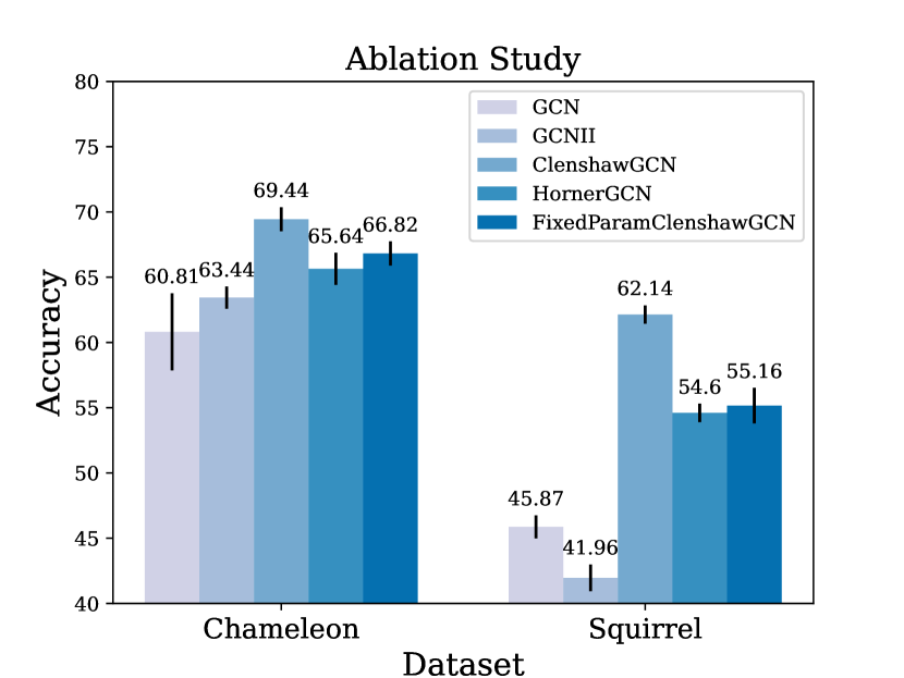
Figure 2. Results of the ablation study. HornerGCN and FixedParamClenshawGCN are weakened versions of ClenshawGCN. HornerGCN is only equipped with adaptive initial residue, and FixedParamClenshawGCN is only equipped with negative second-order residue. The performance of these two ablation models are worse than a complete ClenshawGCN but outperform GCN and GCNII.

figure description

For ClenshawGCN, the core of the design is the two residual connection modules. In this section, we conduct ablation analyses on these two modules to verify their contribution.

Ablation Model: HornerGCN

We use HornerGCN as an ablation model to verify the contribution of negative residues. Recal Theorem 3.1, the corresponding polynomial filter of HornerGCN is

$$h_{Horner}(\mu)=\sum_{\ell=0}^{K}{\alpha}_{K-\ell}\mu^{\ell},$$

which uses the Monomial basis. While the complete form of our ClenshawGCN borrows the use of chebyshev basis by negative residues.

Ablation Model: FixedParamClenshawGCN

In the FixedParamClenshawGCN model, we verify the contribution of adaptive initial residue by fixing $\vec{\alpha}=\left[\hat{\alpha}_{0},\hat{\alpha}_{1},\cdots,\hat{\alpha}_{K}\right]$ with

$$\hat{\alpha}_{\ell}={\alpha}(1-{\alpha})^{K-\ell},\quad\hat{\alpha}_{0}=(1-\alpha)^{K}$$

following APPNP (Klicpera et al., 2019a), where $\alpha\in\left[0,1\right]$ is a hyperparameter. The corresponding polynomial filter of FixedParamClenshawGCN is:

$$h_{Fix}(\mu)=\sum_{\ell=0}^{K}{\hat{\alpha}}_{K-\ell}U_{\ell}(\mu).$$

Analysis

We compare the performance of HornerGCN and FixedParamClenshawGCN with GCN, GCNII and ClenshawGCN on two median-sized datasets: Chameleon and Squirrel. As shown in Figure 2, either removing the negative second-order residue or fixing the initial residue causes an obvious drop in Test Accuracy.

Noticeably, with only one residual module, HornerGCN and FixedParamClenshawGCN still outperform homophilic models such as GCNII. For HornerGCN, the reason is obvious: HornerGCN simulates any polynomial filter, which is favorable for heterophilic graphs. For FixedParamClenshawGCN, though the coefficients of $U_{\ell}(\mu)$ are fixed, the contribution of each fused level (i.e. $\mathbf{\tilde{P}^{\ell}}\mathbf{H}^{*}$) is no longer definitely to be positive as in GCNII since each chebyshev polynomial consists of terms with alternating signs, e.g. $U_{4}(\mathbf{\tilde{P}})=16\mathbf{\tilde{P}}^{4}{\color[rgb]{1,0,0}-}12\mathbf{\tilde{P}}^{2}{\color[rgb]{1,0,0}+}1$, which breaks the underlying homophily assumption.

5. Conclusion

In this paper, we propose ClenshawGCN, a GNN model equipped with a novel and neat residual connection module that is able to mimic a spectral polynomial filter. When generating node representations for the next layer(i.e. $\mathbf{H}^{(\ell+1)}$), our model should only connect to the initial layer(i.e. $\mathbf{H}^{(0)}$) adaptively, and to the second last layer(i.e. $\mathbf{H}^{(\ell-1)}$) negatively. The construction of this residual connection inherently uses Clenshaw Summation Algorithm, a numerical evaluation algorithm for calculating weighted sums of Chebyshev basis. We prove that our model implicitly simulates any polynomial filter based on the second-kind Chebyshev basis entangle with non-linear layers, bringing it at least comparable expressive power with state-of-art polynomial spectral GNNs. Experiments demonstrate our model’s superiority either compared with other spatial models with residual connections or with spectral models.

For future work, a promising direction is to further investigate the mechanism and potential of such spectrally-inspired models entangled with non-linearity, which seems be able to incorporate the strengths of both sides.

References

- (1)
- Abu-El-Haija et al. (2019) Sami Abu-El-Haija, Bryan Perozzi, Amol Kapoor, Nazanin Alipourfard, Kristina Lerman, Hrayr Harutyunyan, Greg Ver Steeg, and Aram Galstyan. 2019. Mixhop: Higher-order graph convolutional architectures via sparsified neighborhood mixing. In international conference on machine learning. PMLR, 21–29.
- Akiba et al. (2019) Takuya Akiba, Shotaro Sano, Toshihiko Yanase, Takeru Ohta, and Masanori Koyama. 2019. Optuna: A next-generation hyperparameter optimization framework. In Proceedings of the 25th ACM SIGKDD international conference on knowledge discovery & data mining. 2623–2631.
- Bianchi et al. (2021) Filippo Maria Bianchi, Daniele Grattarola, Lorenzo Livi, and Cesare Alippi. 2021. Graph neural networks with convolutional arma filters. IEEE Transactions on Pattern Analysis and Machine Intelligence (2021).
- Burt and Adelson (1987) Peter J Burt and Edward H Adelson. 1987. The Laplacian pyramid as a compact image code. In Readings in computer vision. Elsevier, 671–679.
- Chamberlain et al. (2021) Ben Chamberlain, James Rowbottom, Maria I Gorinova, Michael Bronstein, Stefan Webb, and Emanuele Rossi. 2021. Grand: Graph neural diffusion. In International Conference on Machine Learning. PMLR, 1407–1418.
- Chen et al. (2020) Ming Chen, Zhewei Wei, Zengfeng Huang, Bolin Ding, and Yaliang Li. 2020. Simple and deep graph convolutional networks. In ICML. PMLR, 1725–1735.
- Chien et al. (2021) Eli Chien, Jianhao Peng, Pan Li, and Olgica Milenkovic. 2021. Adaptive Universal Generalized PageRank Graph Neural Network. In ICLR.
- Craven et al. (1998) Mark Craven, Andrew McCallum, Dan PiPasquo, Tom Mitchell, and Dayne Freitag. 1998. Learning to extract symbolic knowledge from the World Wide Web. Technical Report. Carnegie-mellon univ pittsburgh pa school of computer Science.
- Defferrard et al. (2016) Michaël Defferrard, Xavier Bresson, and Pierre Vandergheynst. 2016. Convolutional Neural Networks on Graphs with Fast Localized Spectral Filtering. (6 2016). http://arxiv.org/abs/1606.09375
- Duvenaud et al. (2015) David K Duvenaud, Dougal Maclaurin, Jorge Iparraguirre, Rafael Bombarell, Timothy Hirzel, Alán Aspuru-Guzik, and Ryan P Adams. 2015. Convolutional networks on graphs for learning molecular fingerprints. Advances in neural information processing systems 28 (2015).
- Fan et al. (2019) Wenqi Fan, Yao Ma, Qing Li, Yuan He, Eric Zhao, Jiliang Tang, and Dawei Yin. 2019. Graph neural networks for social recommendation. In The world wide web conference. 417–426.
- He et al. (2016) Kaiming He, Xiangyu Zhang, Shaoqing Ren, and Jian Sun. 2016. Deep Residual Learning for Image Recognition. In Proceedings of the IEEE Conference on Computer Vision and Pattern Recognition (CVPR).
- He et al. (2021) Mingguo He, Zhewei Wei, Zengfeng Huang, and Hongteng Xu. 2021. BernNet: Learning Arbitrary Graph Spectral Filters via Bernstein Approximation. Advances in Neural Information Processing Systems 34 (6 2021), 14239–14251. http://arxiv.org/abs/2106.10994
- He et al. (2022) Mingguo He, Zhewei Wei, and Ji-Rong Wen. 2022. Convolutional Neural Networks on Graphs with Chebyshev Approximation, Revisited. arXiv preprint arXiv:2202.03580 (2022).
- Horner (1819) William George Horner. 1819. XXI. A new method of solving numerical equations of all orders, by continuous approximation. Philosophical Transactions of the Royal Society of London 109 (1819), 308–335.
- Iandola et al. (2014) Forrest Iandola, Matt Moskewicz, Sergey Karayev, Ross Girshick, Trevor Darrell, and Kurt Keutzer. 2014. Densenet: Implementing efficient convnet descriptor pyramids. arXiv preprint arXiv:1404.1869 (2014).
- Kingma and Ba (2014) Diederik P Kingma and Jimmy Ba. 2014. Adam: A method for stochastic optimization. arXiv preprint arXiv:1412.6980 (2014).
- Kipf and Welling (2017) Thomas N Kipf and Max Welling. 2017. Semi-supervised classification with graph convolutional networks. In ICLR.
- Klicpera et al. (2019a) Johannes Klicpera, Aleksandar Bojchevski, and Stephan Günnemann. 2019a. Predict then propagate: Graph neural networks meet personalized pagerank. In ICLR.
- Klicpera et al. (2019b) Johannes Klicpera, Stefan Weißenberger, and Stephan Günnemann. 2019b. Diffusion improves graph learning. arXiv preprint arXiv:1911.05485 (2019).
- Li et al. (2019) Guohao Li, Matthias Müller, Ali Thabet, and Bernard Ghanem. 2019. DeepGCNs: Can GCNs Go as Deep as CNNs? (4 2019). http://arxiv.org/abs/1904.03751
- Li et al. (2018) Qimai Li, Zhichao Han, and Xiao-Ming Wu. 2018. Deeper insights into graph convolutional networks for semi-supervised learning. In Thirty-Second AAAI conference on artificial intelligence.
- Lim et al. (2021) Derek Lim, Felix Hohne, Xiuyu Li, Sijia Linda Huang, Vaishnavi Gupta, Omkar Bhalerao, and Ser-Nam Lim. 2021. Large Scale Learning on Non-Homophilous Graphs: New Benchmarks and Strong Simple Methods. Advances in Neural Information Processing Systems 34 (10 2021), 20887–20902. http://arxiv.org/abs/2110.14446
- Liu et al. (2021) Xiaorui Liu, Jiayuan Ding, Wei Jin, Han Xu, Yao Ma, Zitao Liu, and Jiliang Tang. 2021. Graph Neural Networks with Adaptive Residual. NIPS (2021). https://github.com/lxiaorui/AirGNN.
- Luan et al. (2021) Sitao Luan, Chenqing Hua, Qincheng Lu, Jiaqi Zhu, Mingde Zhao, Shuyuan Zhang, Xiao-Wen Chang, and Doina Precup. 2021. Is Heterophily A Real Nightmare For Graph Neural Networks To Do Node Classification? (9 2021). http://arxiv.org/abs/2109.05641
- McPherson et al. (2001) Miller McPherson, Lynn Smith-Lovin, and James M Cook. 2001. Birds of a feather: Homophily in social networks. Annual review of sociology (2001), 415–444.
- Narang et al. (2013) Sunil K Narang, Akshay Gadde, and Antonio Ortega. 2013. Signal processing techniques for interpolation in graph structured data. In 2013 IEEE International Conference on Acoustics, Speech and Signal Processing. IEEE, 5445–5449.
- Paris et al. (2011) Sylvain Paris, Samuel W Hasinoff, and Jan Kautz. 2011. Local laplacian filters: edge-aware image processing with a laplacian pyramid. ACM Trans. Graph. 30, 4 (2011), 68.
- Pei et al. (2020) Hongbin Pei, Bingzhe Wei, Kevin Chen-Chuan Chang, Yu Lei, and Bo Yang. 2020. Geom-GCN: Geometric Graph Convolutional Networks. In ICLR.
- Perozzi and Akoglu (2018) Bryan Perozzi and Leman Akoglu. 2018. Discovering communities and anomalies in attributed graphs: Interactive visual exploration and summarization. ACM Transactions on Knowledge Discovery from Data (TKDD) 12, 2 (2018), 1–40.
- Rong et al. (2020) Yu Rong, Wenbing Huang, Tingyang Xu, and Junzhou Huang. 2020. DropEdge: Towards Deep Graph Convolutional Networks on Node Classification. In ICLR.
- Satorras et al. (2021) Vıctor Garcia Satorras, Emiel Hoogeboom, and Max Welling. 2021. E (n) equivariant graph neural networks. In International conference on machine learning. PMLR, 9323–9332.
- Schlichtkrull et al. (2020) Michael Sejr Schlichtkrull, Nicola De Cao, and Ivan Titov. 2020. Interpreting graph neural networks for nlp with differentiable edge masking. arXiv preprint arXiv:2010.00577 (2020).
- Sen et al. (2008) Prithviraj Sen, Galileo Namata, Mustafa Bilgic, Lise Getoor, Brian Galligher, and Tina Eliassi-Rad. 2008. Collective classification in network data. AI magazine 29, 3 (2008), 93–93.
- Shuman et al. (2013) David I Shuman, Benjamin Ricaud, and Pierre Vandergheynst. 2013. Vertex-Frequency Analysis on Graphs. (7 2013). http://arxiv.org/abs/1307.5708
- Sutskever et al. (2013) Ilya Sutskever, James Martens, George Dahl, and Geoffrey Hinton. 2013. On the importance of initialization and momentum in deep learning. In International conference on machine learning. PMLR, 1139–1147.
- Tang et al. (2009) Jie Tang, Jimeng Sun, Chi Wang, and Zi Yang. 2009. Social influence analysis in large-scale networks. In Proceedings of the 15th ACM SIGKDD international conference on Knowledge discovery and data mining. 807–816.
- Wang et al. (2019) Guangtao Wang, Rex Ying, Jing Huang, and Jure Leskovec. 2019. Improving graph attention networks with large margin-based constraints. arXiv preprint arXiv:1910.11945 (2019).
- Wang and Zhang (2022) Xiyuan Wang and Muhan Zhang. 2022. How Powerful are Spectral Graph Neural Networks. (5 2022). http://arxiv.org/abs/2205.11172
- Wu et al. (2021) Lingfei Wu, Yu Chen, Kai Shen, Xiaojie Guo, Hanning Gao, Shucheng Li, Jian Pei, and Bo Long. 2021. Graph neural networks for natural language processing: A survey. arXiv preprint arXiv:2106.06090 (2021).
- Wu et al. (2020) Shiwen Wu, Fei Sun, Wentao Zhang, Xu Xie, and Bin Cui. 2020. Graph neural networks in recommender systems: a survey. ACM Computing Surveys (CSUR) (2020).
- Xu et al. (2018) Keyulu Xu, Chengtao Li, Yonglong Tian, Tomohiro Sonobe, Ken-ichi Kawarabayashi, and Stefanie Jegelka. 2018. Representation Learning on Graphs with Jumping Knowledge Networks. In ICML.
- Yang et al. (2022) Liang Yang, Weihang Peng, Wenmiao Zhou, Bingxin Niu, Junhua Gu, Chuan Wang, Yuanfang Guo, Xiaochun Cao, and Dongxiao He. 2022. Difference Residual Graph Neural Networks. ACMMM22 (2022). https://doi.org/10.1145/3503161.3548111
- Yang et al. (2016) Zhilin Yang, William Cohen, and Ruslan Salakhudinov. 2016. Revisiting semi-supervised learning with graph embeddings. In International conference on machine learning. PMLR, 40–48.
- Zhang et al. (2022) Wentao Zhang, Zeang Sheng, Ziqi Yin, Yuezihan Jiang, Yikuan Xia, Jun Gao, Zhi Yang, and Bin Cui. 2022. Model Degradation Hinders Deep Graph Neural Networks. Proceedings of the 28th ACM SIGKDD Conference on Knowledge Discovery and Data Mining, 2493–2503. https://doi.org/10.1145/3534678.3539374
- Zhao et al. (2021) Jialin Zhao, Yuxiao Dong, Ming Ding, Evgeny Kharlamov, and Jie Tang. 2021. Adaptive Diffusion in Graph Neural Networks. Advances in Neural Information Processing Systems 34 (2021), 23321–23333.
- Zheng et al. (2022) Xin Zheng, Yixin Liu, Shirui Pan, Miao Zhang, Di Jin, and Philip S Yu. 2022. Graph neural networks for graphs with heterophily: A survey. arXiv preprint arXiv:2202.07082 (2022).
- Zhu et al. (2020) Jiong Zhu, Yujun Yan, Lingxiao Zhao, Mark Heimann, Leman Akoglu, and Danai Koutra. 2020. Beyond homophily in graph neural networks: Current limitations and effective designs. Advances in Neural Information Processing Systems 33 (2020), 7793–7804.