HectoMAP: The Complete Redshift Survey (Data Release 2)

Abstract

HectoMAP is a dense redshift survey of 95,403 galaxies based primarily on MMT spectroscopy with a median redshift $z=0.345$. The survey covers 54.64 square degrees in a 1.5^∘ wide strip across the northern sky centered at a declination of 43.25^∘. We report the redshift, the spectral indicator ${\rm D}_{n}4000$, and the stellar mass. The red selected survey is 81% complete for 55,962 galaxies with $(g-r)>1$ and $r<20.5$; it is 72% complete for 32,908 galaxies with $(g-r)>1$, $(r-i)>0.5$ and $20.5<r<21.3$. Comparison of the survey basis SDSS photometry with the HSC-SSP photometry demonstrates that HectoMAP provides complete magnitude limited surveys based on either photometric system. We update the comparison between the HSC-SSP photometric redshifts with HectoMAP spectroscopic redshifts; the comparison demonstrates that the HSC-SSP photometric redshifts have improved between the second and third data releases. HectoMAP is a foundation for examining the quiescent galaxy population (63% of the survey), clusters of galaxies, and the cosmic web. HectoMAP is completely covered by the HSC-SSP survey, thus enabling a variety of strong and weak lensing investigations.

1 INTRODUCTION

The universe of redshift surveys has undergone enormous expansion since the early surveys (e.g., Davis et al., 1982; Geller & Huchra, 1989; Shectman et al., 1996). Digital detectors enabled these pioneering surveys. Ever increasing multiplexing enabled by the combination of robotics and fiber optics underlies current and upcoming impressive projects: GAMA (Robotham et al., 2010; Liske et al., 2015), WEAVE (Dalton et al., 2012), Subaru/PFS (Takada et al., 2014), 4MOST (Richard et al., 2019), DEVILS (Davies et al., 2018), MOONRISE (Maiolino et al., 2020) and DESI (Hahn et al., 2022).

Hectospec, a 300-fiber robotic instrument (Fabricant et al., 2005) mounted on the 6.5-meter MMT has contributed significantly to redshift surveys covering the range $0.2<z<0.8$ (Kochanek et al., 2012; Geller et al., 2014, 2016; Damjanov et al., 2018). SHELS (Geller et al., 2016) is a magnitude-limited redshift survey of two Deep Lensing Survey fields (Wittman et al., 2006) without any color selection. Damjanov et al. (2022a) use SHELS to calibrate the much larger red-selected HectoMAP survey. HectoMAP is a dedicated redshift survey using Hectospec to study galaxies in the redshift range $0.2<z<0.6$. We follow the Damjanov et al. (2022a) approach in further highlighting the completeness of the HectoMAP sample of quiescent galaxies.

The full HectoMAP survey covers 54.64 square degrees in a 1.5^∘ wide strip centered at a declination of 43.25^∘. The red-selected survey is designed to provide dense sampling of the quiescent galaxy population (Damjanov et al., 2022b), clusters of galaxies (Sohn et al., 2018a, b, 2021a), and the cosmic web (Hwang et al., 2016). The average survey density is $\sim 1800$ galaxies deg^-2 and the median redshift $z=0.345$. Pizzardo et al. (2022) demonstrate that this sampling positions HectoMAP as the foundation for a direct measurement of the galaxy cluster growth rate over the last 7 gigayears of cosmic history.

Sohn et al. (2021b) is the first HectoMAP data release (DR1 hereafter). DR1 covers 8.7 deg² and includes 17,313 galaxies. As demonstrations of the broad scientific applications of HectoMAP, the paper includes an assay of redMaPPer clusters (Rykoff et al., 2016) in the region and a test of the HSC DeMP photometric redshifts (Hsieh & Yee, 2014).

The availability of HSC-SSP $grizy$ photometry (Aihara et al., 2022) covering the entire HectoMAP region also distinguishes the survey and enables investigations that combine two of the powerful tools of modern cosmology, redshift surveys and weak lensing. HectoMAP promises a platform for these combined studies ranging from the masses of galaxies to the relationship between the galaxy and dark matter distributions on large scales. Damjanov et al. (2022b) also highlight the power of the completeness of the HectoMAP quiescent sample combined with sizes from HSC-SSP photometry for elucidating the evolution of the size-mass relation for the quiescent population in the redshift range $0.2<z<0.6$.

Here we describe the full HectoMAP redshift survey data including 95,403 galaxies in the entire 54.64 square degree region of HectoMAP; 88294 ($\sim 93\%)$ of these redshifts are MMT Hectospec observations. Selection for the complete HectoMAP sample is based on SDSS DR16 (Ahumada et al., 2020) photometry: $(g-r)>1$ for $r\leq 20.5$. For $20.5<r\leq 21.3$, we include an additional constraint, $(r-i)>0.5$. We also provide ${\rm D}_{n}4000$ and the stellar mass for most of galaxies with spectroscopy.

We describe the data in Section 2. Section 2.1 reviews the photometric basis for the survey. Section 2.2 describes the HectoMAP spectroscopy, including the MMT spectroscopy (Section 2.2.2) that provides the vast majority of the spectroscopic data. Section 3 includes the survey catalog. Sections 3.1 and 3.2 describe the ${\rm D}_{n}4000$ and stellar mass, respectively. We include the full HectoMAP catalog in Section 3.4. The red-selected survey and the subset of quiescent galaxies are highly complete (Section 4). Section 5 compares the SDSS and HSC-SSP photometry in the region, and Section 6 compares updated photometric redshifts based on HSC-SSP DR3 photometry (Aihara et al., 2022) with HectoMAP spectroscopic redshifts. Section 7 highlights past and future applications of HectoMAP including a brief discussion of strong lensing clusters in the region. We conclude in Section 8. We use the Planck cosmological parameters: $H_{0}=67.74~{}{\rm km~{}s^{-1}~{}Mpc^{-1}}$, $\Omega_{m}=0.3089$, and $\Omega_{\Lambda}=0.6911$ throughout.

2 THE DATA

HectoMAP is a large, deep, dense redshift survey enabling investigation of the quiescent galaxy population, clusters of galaxies, and large-scale structure in the redshift range $0.2<z<0.6$. HectoMAP covers a 54.64 square degree region within a narrow strip across the northern sky: $200<$ R.A. (deg) $<250$ and $42.5<$ Decl. (deg) $<44.0$. Data Release 1 (DR1) (Sohn et al., 2021b) includes photometric and spectroscopic properties of galaxies in the region $242<$ R.A. (deg) $<250$. Here, we include the complete redshift sample for HectoMAP.

We first describe the photometric and spectroscopic basis for the HectoMAP spectroscopic catalog. The photometric data (Section 2.1) include the survey basis from SDSS (Section 2.1.1) and the later much deeper Subaru HSC/SSP photometry (Section 2.1.2). We next describe the HectoMAP spectroscopy (Section 2.2). SDSS spectroscopy provides a low redshift sample (Section 2.2.1). MMT observations with Hectospec provide the vast majority of the spectroscopy (Section 2.2.2).

2.1 Photometry

2.1.1 SDSS Photometry

Galaxy selection for the HectoMAP spectroscopic survey is based on SDSS DR16 photometry (Ahumada et al., 2020). We selected galaxies with $probPSF=0$, where $probPSF$ gives the probability that the object is a star. We applied additional object selection criteria based on the SDSS photometric flags to remove spurious sources, including stellar bleeding, suspicious detections, objects with deblending problems, and objects without proper Petrosian photometry. There are 212,120 galaxies with $r\leq 21.3$, the magnitude limit of HectoMAP.

We base the survey on SDSS $ugriz$ Petrosian magnitudes after foreground extinction correction. We also obtain colors based on model magnitudes following our previous spectroscopic surveys (e.g., F2, Geller et al., 2014). Petrosian magnitudes are galaxy fluxes measured within a circular aperture with a radius defined by the azimuthally averaged light profile (Petrosian, 1976). SDSS photometry provides galaxy fluxes resulting from fits of de Vaucouleur and exponential models. Model magnitudes select the better of these two fits in the $r-$band as a basis for calculating the flux in all bands. Hereafter, $r_{petro,0}$ refers to the SDSS Petrosian magnitude corrected for foreground extinction. The SDSS model colors, $(g-r)_{model,0}$ and $(r-i)_{model,0}$, are also corrected for foreground extinction. Hereafter, we designate $r=r_{petro,0}$, $(g-r)=(g-r)_{model,0}$, and $(r-i)=(r-i)_{model,0}$ in the text; we retain the full notation in the figure captions for clarity.

Additionally, we compile the composite model (cModel) magnitudes. The cModel magnitudes are based on a linear combination of the best fitting exponential and de Vaucouleurs models (Strauss et al., 2002). For galaxies, cModel magnitudes agree well with Petrosian magnitudes. We use cModel magnitudes for comparison with the much deeper HSC-SSP photometry (Section 5) where similarly defined cModel magnitudes are available.

2.1.2 Subaru/HSC Photometry

HectoMAP is covered by the HSC-SSP wide survey (Miyazaki et al., 2012), which provides deep photometry to a $5\sigma$ depth of 26.5, 26.5, 26.2, 25.2, and 24.4 mag in the $g$, $r$, $i$, $z$, and $y$-bands for point sources, respectively (Aihara et al., 2022). We use the HSC-SSP Public Data Release 3 (hereafter HSC-SSP DR3, Aihara et al., 2022) to explore the relationship between the SDSS and Subaru photometry (Section 5). The HSC-SSP DR3 includes the complete HectoMAP survey region in the $g,r$ and $z$ bands; the survey for $i$ and $y$ bands are $\sim 80\%$ complete.

We use the ‘forced’ DR3 catalog that lists forced photometry on coadded images. The forced DR3 photometry is based on the set of images generated with a local sky subtraction scheme (Aihara et al., 2022). In the catalog, there are two types of photometry: Kron and cModel magnitudes. We use cModel magnitudes (Bosch et al., 2018) for direct comparison with the cModel magnitudes from SDSS. The cModel photometry yields unbiased color estimates (Huang et al., 2018b).

We match the HSC-SSP catalog to the SDSS photometric catalog with a matching tolerance of $1\arcsec$. Most of the SDSS galaxies have HSC counterparts (93%). The SDSS objects missing from HSC photometry are mostly near bright saturated stars in the HSC images. We discuss the comparison between HSC and SDSS photometry in Section 5.

2.2 Spectroscopy

The HectoMAP survey includes redshifts for 95,403 unique galaxies; 88,294 of these redshifts are MMT/Hectospec observations (Section 2.2.2). Particularly at redshifts $z<0.2$, SDSS complements the HectoMAP data (Section 2.2.1). The NASA Extragalactic Database adds only a few (375) unique redshifts in the HectoMAP survey region.

Table 1 summarizes spectroscopic redshifts from different sources in various subsamples. The first line of Table 1 includes the stars discussed in Appendix. All other entries are samples of galaxies.

Table 1: HectoMAP Survey Subsets

Subsample	$N_{phot}$	$N_{spec,MMT}$	$N_{spec,SDSS/BOSS}$	$N_{spec,NED}$	$N_{spec,total}$	$f_{complete}$
Entire sample with spectroscopy∗ ($r\leq 23$)	$\cdots$	94114	19538	464	114116	$\cdots$
Galaxies with $r\leq 23$	$\cdots$	88294	6734	375	95403	$\cdots$
Galaxies within $21.3<r\leq 23$	$\cdots$	6095	4555	0	10650	$\cdots$
Main ($r\leq 21.3$))	212120	82610	5560	326	88496	41.72
Main ($(g-r)>1.0$)	108555	69788	2777	54	72619	66.90
Main ($(g-r)>1.0$ & $(r-i)>0.5$)	65729	52985	1923	5	54913	83.54
Main ($(g-r)\leq 1.0$)	103565	12822	2783	205	15810	15.27
Bright ($r\leq 20.5$)	107166	54983	4614	312	59909	55.90
Bright ($r\leq 20.5$)	55963	43435	1921	51	45407	81.14
Bright ($(g-r)>1.0$ & $(r-i)>0.5$)	32821	30072	1069	3	31144	94.89
Bright ($(g-r)\leq 1.0$)	51203	11548	2693	195	14436	28.19
Faint ($20.5<r\leq 21.3$)	104954	27627	946	14	28587	27.24
Faint ($(g-r)>1.0$)	52592	26353	856	3	27212	51.74
Faint ($(g-r)>1.0$ & $(r-i)>0.5$)	32908	22913	854	2	23769	72.23
Faint ($(g-r)\leq 1.0$)	52362	1274	90	11	1375	2.63

2.2.1 SDSS Spectroscopy

The SDSS main galaxy sample is a complete spectroscopic survey ($\sim 90-95\%$ complete, Strauss et al., 2002; Lazo et al., 2018) for galaxies with $r<17.77$. We include 3932 unique SDSS main galaxy sample redshifts in the HectoMAP catalog. The SDSS spectra cover the wavelength range 3700 - 9100 Å with a typical spectral resolution of $\sim 3~{}{\rm\AA}$. The typical uncertainty of the SDSS redshifts we use is $8~{}\rm km~{}s^{-1}$.

There are also 2802 unique SDSS/BOSS redshifts in the HectoMAP region. BOSS spectra cover the wavelength range $3600-10400{\rm\AA}$. Because BOSS typically targets fainter and higher redshift objects, the uncertainty in the BOSS redshifts is generally larger ($\sim 39~{}\rm km~{}s^{-1}$) than for the SDSS redshifts.

The purple histograms in Figures 1 (a) and (b) show the distributions of $r-$band magnitudes and redshifts for the MMT/Hectospec galaxies (Section 2.2.2) in HectoMAP. Blue-hatched and red-open histograms display the small contribution to the overall survey from unique galaxies in SDSS and BOSS, respectively. The SDSS Main Galaxy Sample is limited to $z<0.2$. Less than 1% of the entire HectMAP spectroscopic sample is from SDSS. BOSS reaches fainter magnitudes ($r>18$) and thus covers a wider redshift range; BOSS contributes $\sim 3\%$ of the HectoMAP spectroscopy.

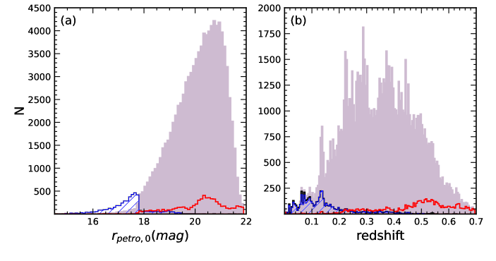
Figure 1: (a) Distribution of $r_{petro,0}$ for MMT/Hectospec (purple filled), SDSS (blue hatched), BOSS (red open) galaxies in HectoMAP. (b) Same as (a), but for the redshift distributions.

2.2.2 MMT/Hectospec Spectroscopy

We used MMT/Hectospec (Fabricant et al., 2005) to obtain spectroscopy for most of the galaxies in HectoMAP. Hectospec has 300 fibers each with a $1.5\arcsec$ aperture. A single observation generally acquires spectra for $\sim 250$ galaxies over the 1 degree diameter field of view of the instrument; the remaining fibers observe the sky. The 270 mm^-1 Hectospec grating yields a typical resolution of $\sim 6~{}{\rm\AA}$ and covers the wavelength range 3700 - 9100 Å. We made HectoMAP observations from 2009 January to 2019 May.

HectoMAP is a red-selected survey. We targeted brighter galaxies with $r\leq 20.5$ and $(g-r)>1.0$. For fainter galaxies with $20.5<r\leq 21.3$, we applied an additional color selection $(r-i)>0.5$ to complete the survey within the limited available telescope time. Conducting a magnitude-limited survey without color selection was prohibitive. We discuss the survey completeness in Section 4.

We reduced the Hectospec spectra using the standard pipeline, HSRED v2.0. We derive redshifts based on the cross-correlation tool, RVSAO (Kurtz & Mink, 1998). RVSAO yields the cross-correlation score ($R_{XC}$). Following previous Hectospec surveys, we take the $R_{XC}>3$ (see Figure 3 of Sohn et al. (2021b)) as a reliable redshift (Rines et al., 2016; Sohn et al., 2021b). The typical redshift uncertainty in a Hectospec redshift is $\sim 39~{}\rm km~{}s^{-1}$, comparable with the uncertainty in BOSS redshifts.

There are 924/4496 galaxies that have both Hectospec and SDSS/BOSS spectra. The Hectospec redshifts are slightly lower than the SDSS/BOSS redshifts: $c\Delta(z_{SDSS/BOSS}-z_{Hecto})/(1+z_{Hecto})=42~{}\rm km~{}s^{-1}$. Sohn et al. (2021b) explored this issue in detail by showing the redshift difference as a function of the signal-to-noise (S/N) ratio of the spectra (see their Figure 6). Here, we note that the redshift difference is comparable to the typical uncertainty in a Hectospec redshift. The systematic difference does not affect any of the analysis we carry out here.

3 The HectoMAP Spectroscopic Catalog

Based on the photometric and spectroscopic data for the HectoMAP region, we derive several spectroscopic properties of the galaxies. We outline the spectroscopic properties including ${\rm D}_{n}4000$ (Section 3.1), stellar mass ($M_{*}$, Section 3.2), and K-correction (Section 3.3). We describe the complete HectoMAP spectroscopic DR2 catalog in Section 3.4.

3.1 ${\rm D}_{n}4000$

We derive the spectral indicator ${\rm D}_{n}4000$ that measures the flux ratio around the $4000~{}{\rm\AA}$ break. The ${\rm D}_{n}4000$ index is a useful and robust tracer of the age of stellar population of galaxies. For example, Kauffmann et al. (2003) show that ${\rm D}_{n}4000$ increases monotonically after a burst of star formation (see also Zahid et al., 2019). This index is also useful for identifying the quiescent galaxy population (e.g., Vergani et al., 2008; Zahid et al., 2016; Sohn et al., 2017a, b; Damjanov et al., 2022b; Hamadouche et al., 2022). We use ${\rm D}_{n}4000$ to select quiescent galaxies in HectoMAP.

We compute the flux ratio between two spectral windows $3850-3950~{}{\rm\AA}$ and $4000-4100~{}{\rm\AA}$ following the definition from Balogh et al. (1999). The median signal-to-noise ratio at $3850-4100{\rm\AA}$ is $\sim 4.5$. We measure the ${\rm D}_{n}4000$ for 99% of HectoMAP objects with spectroscopy. The missing ${\rm D}_{n}4000$ objects are the few galaxies with a NED redshift where we do not have a spectrum. Table 2 summarizes the fraction of galaxies with ${\rm D}_{n}4000$ measurements and with ${\rm D}_{n}4000>1.5$.

Figure 2 (a) shows the ${\rm D}_{n}4000$ absolute error as a function of ${\rm D}_{n}4000$. The typical ${\rm D}_{n}4000$ uncertainties measured from SDSS, BOSS, and Hectospec spectra are 0.04, 0.10, and 0.07, respectively. We also compare the difference between ${\rm D}_{n}4000$ measured from Hectospec and ${\rm D}_{n}4000$ measured from SDSS/BOSS. The mean ${\rm D}_{n}4000$ difference is very small, i.e., $\Delta{\rm D}_{n}4000~{}{\rm(Hecto-SDSS/BOSS)}=-0.014\pm 0.003$.

Figure 2 (b) displays the ${\rm D}_{n}4000$ distribution. We overlay the red-selected galaxies with $(g-r)>1.0$ (blue hatched histogram) and $(g-r)>1.0$ and $(r-i)>0.5$ (red open histogram), respectively. The ${\rm D}_{n}4000$ distribution of HectoMAP galaxies is bimodal; the larger ${\rm D}_{n}4000$ population is quiescent. We identify quiescent galaxies with ${\rm D}_{n}4000\geq 1.5$ following previous MMT surveys. Overall, 63% of HectoMAP galaxies are quiescent. This large quiescent fraction results from the red-selection of the survey.

Figure 2: (a) ${\rm D}_{n}4000$ absolute error vs. ${\rm D}_{n}4000$ for HectoMAP galaxies. Redder color indicates higher number density. (b) The ${\rm D}_{n}4000$ distribution of all HectoMAP galaxies (black filled histogram), galaxies with $(g-r)>1.0$ (blue hatched), and galaxies with $(g-r)>1.0$ and $(r-i)>0.5$ (red open).

Table 2: Completeness of ${\rm D}_{n}4000$ and Stellar Mass Measurements

Subsample		$N_{sample}$	$f_{{\rm D}_{n}4000}$	$f_{M_{*}}$	$f_{{\rm D}_{n}4000>1.5}$
All Galaxies,		95403	0.9996	0.9946	0.6314
$r\leq 20.5$,	$(g-r)>1.0$	45407	0.9994	0.9977	0.7699
$r\leq 20.5$,	$(g-r)>1.0~{}\&(r-i)>0.5$	31147	0.9995	0.9986	0.8226
$20.5<r\leq 21.3$,	$(g-r)>1.0$	27212	0.9999	0.9988	0.6425
$20.5<r\leq 21.3$,	$(g-r)>1.0~{}\&(r-i)>0.5$	23769	1.0000	0.9989	0.6872

3.2 Stellar Mass

We compute the stellar masses of galaxies as we did for previous MMT/Hectospec redshift surveys (e.g., Geller et al., 2014; Zahid et al., 2016; Sohn et al., 2017a, 2021b; Damjanov et al., 2022b). We use foreground-extinction corrected SDSS $ugriz$ model magnitudes to compute the stellar mass. We use the Le PHARE fitting code (Arnouts et al., 1999; Ilbert et al., 2006) to fit the observed and model spectral energy distributions (SEDs). To generate model SEDs, we employ the stellar population synthesis models of Bruzual & Charlot (2003). We assume a universal Chabrier initial mass function (Chabrier, 2003) and two metallicities. We also consider a set of models with exponentially declining star formation rates with e-folding times for the star formation ranging from 0.1 to 30 Gyr. We also consider the internal extinction range $E(B-V)=0-0.6$ using the extinction law from Calzetti et al. (2000). The model SEDs are normalized to solar luminosity, and the ratio between the observed and model SEDs is the stellar mass. The median of the best-fit stellar mass distribution is the stellar mass we use.

Figure 3 (a) shows the distribution of stellar masses for galaxies in the HectoMAP survey. The red selection of HectoMAP shifts the survey toward galaxies with generally high stellar mass. The stellar mass range is $8.0<\log(M_{*}/M_{\odot})<12.0$. The typical stellar mass uncertainty is $\Delta\log(M_{*}/M_{\odot})\sim 0.12\pm 0.33$. We note that stellar mass estimates based on broad band photometry can also have systematic uncertainties of $\sim 0.3$ dex (e.g., Conroy et al., 2009).

Figure 3 (b) displays the stellar mass as a function of redshift. As expected in a magnitude-limited survey, there are more low mass galaxies at low redshift. Figure 3 (c) shows ${\rm D}_{n}4000$ versus stellar mass. The low mass objects are mostly star-forming galaxies with low ${\rm D}_{n}4000$. High mass objects generally have larger ${\rm D}_{n}4000$. This behavior is well-known (e.g., Kauffmann et al., 2004; Blanton & Moustakas, 2009).

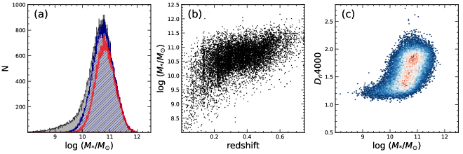
Figure 3: (a) Stellar mass ($M_{*}$) distribution for all HectoMAP galaxies (black filled histogram), galaxies with $(g-r)>1.0$ (blue hatched), and galaxies with $(g-r)>1.0$ and $(r-i)>0.5$ (red open). (b) $M_{*}$ as a function of redshift. (b) ${\rm D}_{n}4000$ as a function of $M_{*}$. We show only 10% of the HectoMAP objects for clarity in panels (b) and (c).

3.3 K-correction

We calculate the K-correction based on the kcorrect IDL package (Blanton & Roweis, 2007). We derive the K-correction at $z=0.35$, the median redshift of HectoMAP to minimize the K-correction we apply. Figure 4 (a) displays the K-correction distribution as a function of redshift. The K-correction at $z=0.35$ is $-0.31$. The dashed line shows the median K-correction as a function of redshift. The best-fit median K-correction is:

$$K_{r}=-0.31+1.75(z-0.35)+3.58(z-0.35)^{2}.$$ (1)

Figure 4 (b) shows the K-corrected $r-$band absolute magnitude of HectoMAP galaxies as a function of redshift. Two dashed lines show the $r=20.5$ and $r=21.3$ magnitude limits shifted by the median K-correction (equation 1). These lines are useful for deriving volume-limited subsamples within HectoMAP.

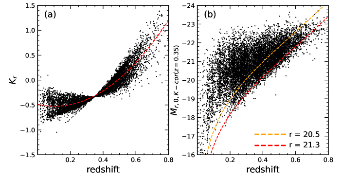
Figure 4: (a) $r-$band K-correction as a function of redshift. Red dashed line shows the best-fit polynomial fit for the median K-correction. (b) The K-corrected $r-$band absolute magnitude as a function of redshift. Yellow and red dashed lines show the $r=20.5$ and $r=21.3$ magnitude limits shifted by the median K-correction, respectively. We plot only $10\%$ of randomly sampled HectoMAP galaxies for clarity. We apply no color selection here.

3.4 The HectoMAP Spectroscopic Catalog

Table 3 lists the 95,403 galaxies with spectroscopy in the full 54.64 deg² HectoMAP region. Table 4 in the Appendix lists the 6544 stars observed in the HectoMAP spectroscopic campaign. Among these stars, 2291 objects were identified as galaxies ($probPSF=0$) in the SDSS photometric database.

Table 3 includes the SDSS Object ID (Column 1), Right Ascension (Column 2), Declination (Column 3), the redshift and its uncertainty (Column 4), the SDSS $r-$band Petrosian magnitude and its uncertainty (Column 5), the K-corrected $r-$band absolute cModel magnitude (Column 6), the SDSS $r-$band cModel magnitude and its uncertainty (Column 7). We also list the HSC-SSP $r-$band cModel magnitude (Column 8). We use the HSC photometry as a basis for the Subaru/SDSS photometric comparison and for estimating the survey completeness based on HSC photometry. We list ${\rm D}_{n}4000$ and its uncertainty (Column 9), the stellar mass and its uncertainty (Column 10), and the source of the spectroscopy (Column 11).

Figure 5 displays a cone diagram for the HectoMAP region based only on SDSS/BOSS spectroscopy. The SDSS spectroscopic survey reveals the characteristic large-scale structure at $z<0.18$; the survey density drops dramatically at higher redshift. The BOSS spectroscopic survey adds redshifts at $z>0.5$. However, the number density is low.

Figure 6 shows a cone diagram for all 95,403 galaxies in HectoMAP. In contrast with Figure 5, the characteristic filaments, walls and voids are strikingly evident. Expanding the figure also reveals the fingers that indicate the central regions of massive clusters. The red points mark the centers of the friends-of-friends clusters identified by Sohn et al. (2021a). The median redshift of the survey is $z=0.345$. Beyond this redshift, the survey density declines as expected for a magnitude-limited survey.

Table 3: The HectoMAP Redshift Survey

SDSS Object ID	R.A.	Decl.	redshift	$r_{petro,0}$	$M_{r,K-cor}^{*}$	$r_{cModel,SDSS,0}$	$r_{cModel,HSC,0}$	${\rm D}_{n}4000$	$\log~{}(M_{*}/{\rm M}_{\odot})$	z Source
	(deg)	(deg)		(mag)	(mag)	(mag)	(mag)
1237661850937262105	200.000865	43.924572	$0.201490\pm 0.000095$	$19.12\pm 0.04$	-20.52	$19.03\pm 0.02$	$18.70\pm 0.01$	$1.47\pm 0.06$	$10.28\pm^{0.23}_{0.12}$	MMT
1237661850400391774	200.000936	43.526926	$0.197847\pm 0.000229$	$20.45\pm 0.09$	-19.05	$20.40\pm 0.05$	$20.24\pm 0.01$	$1.51\pm 0.09$	$9.93\pm^{0.17}_{0.18}$	MMT
1237662196141916862	200.001328	42.629571	$0.481113\pm 0.000100$	$21.08\pm 0.16$	-21.08	$21.06\pm 0.07$	$20.90\pm 0.01$	$1.28\pm 0.07$	$10.30\pm^{0.24}_{0.24}$	MMT
1237661850937262450	200.001377	43.906918	$0.394855\pm 0.000217$	$21.22\pm 0.17$	-20.28	$21.23\pm 0.07$	$21.06\pm 0.01$	$1.90\pm 0.28$	$10.61\pm^{0.11}_{0.15}$	MMT
1237661968508649886	200.001869	42.574824	$0.359950\pm 0.000095$	$19.44\pm 0.02$	-21.75	$19.43\pm 0.02$	$19.44\pm 0.01$	$1.75\pm 0.03$	$11.13\pm^{0.08}_{0.14}$	MMT
1237661871871426772	200.002381	43.335269	$0.230043\pm 0.000105$	$17.83\pm 0.03$	-21.98	$17.89\pm 0.01$	$18.40\pm 0.01$	$1.77\pm 0.04$	$11.32\pm^{0.07}_{0.12}$	MMT
1237661872408298189	200.002811	43.608926	$0.360782\pm 0.000162$	$20.15\pm 0.07$	-21.14	$20.03\pm 0.03$	$19.91\pm 0.01$	$1.49\pm 0.08$	$10.60\pm^{0.13}_{0.14}$	MMT
1237661871334621428	200.007639	42.860764	$0.181610\pm 0.000062$	$18.35\pm 0.03$	-20.97	$18.20\pm 0.01$	$17.96\pm 0.01$	$1.75\pm 0.04$	$11.10\pm^{0.07}_{0.06}$	MMT
1237661871334621440	200.007805	42.789304	$0.228879\pm 0.000145$	$18.25\pm 0.02$	-21.76	$18.21\pm 0.01$	$17.66\pm 0.01$	$1.55\pm 0.03$	$10.57\pm^{0.14}_{0.10}$	MMT
1237661849863586400	200.007981	43.105365	$0.503889\pm 0.000104$	$20.34\pm 0.08$	-22.12	$20.28\pm 0.05$	$19.85\pm 0.01$	$1.55\pm 0.10$	$10.89\pm^{0.16}_{0.19}$	MMT

Notes. The entire table is available in machine-readable form in the online journal. Here, a portion is shown for guidance regarding its format.

Figure 5: HectoMAP cone diagram based only on SDSS/BOSS spectroscopic redshifts. Individual points show galaxies with SDSS/BOSS spectra.

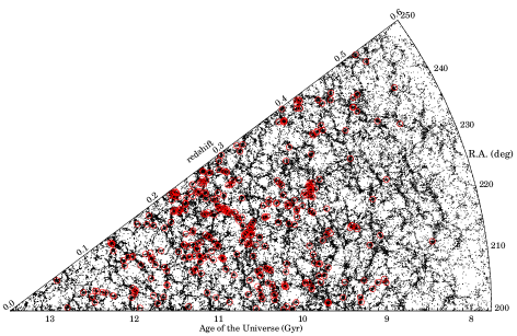
Figure 6: HectoMAP cone diagram for the entire HectoMAP survey. The characteristic filaments and voids of the cosmic web are obvious. Red points mark the centers of friends-of-friends galaxy clusters in Sohn et al. (2021a).

4 Survey Completeness

Survey completeness is a key aspect of a redshift survey. HectoMAP provides a uniform and complete spectroscopic survey for red-selected galaxies in the survey area. The complete HectoMAP survey enables, for example, the identification of galaxy clusters and investigation of quiescent galaxy evolution (e.g., Sohn et al., 2021a; Damjanov et al., 2022a). We evaluate the general HectoMAP survey completeness in Section 4.1 and the HectoMAP survey completeness for quiescent galaxies in Section 4.2.

4.1 HectoMAP Completeness

Figure 7 show (a) the differential spectroscopic survey completeness and (b) the cumulative completeness as a function of $r-$band cModel magnitude. Although the original HectoMAP survey is based on Petrosian magnitudes, we use cModel magnitudes here for direct comparison with the completeness we compute based on HSC-SSP cModel magnitudes (Section 5). In Figure 7, the black solid line shows the completeness for the red-selected sample with $(g-r)>1.0$. The red-selected sample is more than 80% complete (the cumulative completeness) for $r\leq 20.5$ and 67% complete for $r\leq 21.3$. With the additional survey color selection, $(r-i)>0.5$ (red dashed line in Figure 9), HectoMAP is $\sim 95\%$ and $\sim 83\%$ for $r\leq 20.5$ and for $r\leq 21.3$, respectively.

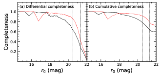
Figure 7: (a) Differential and (b) cumulative completeness of the HectoMAP spectroscopic survey as a function of $r_{cModel,0}$. Black solid and red dashed lines show the completeness for galaxies with $(g-r)>1.0$, and for galaxies with $(g-r)>1.0$ and $(r-i)>0.5$, respectively.

Figure 8 (a) displays the survey completeness map for galaxies brighter than $r=20.5$ and redder than $(g-r)=1.0$. We also display maps for red galaxies with $(g-r)>1.0$ and $(r-i)>0.5$ (Figure 8 (b)). Finally, we show the completeness map for the galaxies with $r\leq 21.3$, $(g-r)>1.0$ and $(r-i)>0.5$ (Figure 8 (c)). A lighter color indicates higher completeness.

HectoMAP is uniformly complete over the entire survey field in general, but the completeness decreases toward the edges of the survey. For example, the completeness for a strip covering the central 0.05 degree declination area is $\sim 90\%$; a similar strip that covers the edge is $\sim 75\%$ complete. The survey is also slightly more complete for $240<$ R.A. (deg) $<242$. This area is the GTO2deg² field (Kurtz et al., 2012) where we tested the feasibility of HectoMAP. Because observing conditions were better when we observed the GTO field, we were able to make 12 visits per unit area in the allocated time rather than the 9 average visits that characterize the full survey.

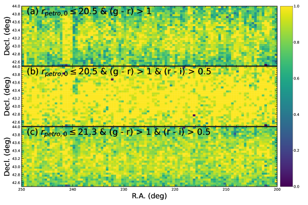
Figure 8: Completeness map for (a) bright galaxies with $r\leq 20.5$ and $(g-r)>1.0$, (b) bright galaxies with $r\leq 20.5$, $(g-r)>1.0$ and $(r-i)>0.5$, and (c) faint galaxies with $r\leq 21.3$, $(g-r)>1.0$, and $(r-i)>0.5$. A lighter color indicates higher completeness. HectoMAP is uniformly complete over the survey area, but the completeness decreases toward the survey declination edges.

4.2 HectoMAP Quiescent Galaxy Completeness

Because HectoMAP is red-selected, the survey is a robust platform for studying the quiescent galaxy population. For example, Damjanov et al. (2022a) explore the size-mass relation of quiescent galaxies. They identify newcomers that join the quiescent population at $z\lesssim 0.5$. Damjanov et al. (2022a) demonstrate that these newcomers typically have larger size at a given stellar mass than their older counterparts. The high completeness of the HectoMAP survey minimizes systematic biases that may originate from incompleteness. HectoMAP enables the definition of complete mass-limited subsamples of the survey. Here we highlight the completeness of the HectoMAP quiescent population.

Following previous work (e.g., Vergani et al., 2008; Zahid et al., 2016; Sohn et al., 2021b; Damjanov et al., 2022b; Hamadouche et al., 2022), we identify quiescent galaxies based on the spectral indicator ${\rm D}_{n}4000$. We identify ${\rm D}_{n}4000>1.5$ galaxies as the quiescent population (Woods et al., 2010; Damjanov et al., 2022b). Here we test the impact of the HectoMAP red-selection on the completeness of the quiescent population by comparing HectoMAP with SHELS/F2 (Damjanov et al., 2022a).

The SHELS/F2 survey (hereafter F2, Geller et al., 2014) provides a unique opportunity for testing the completeness of the HectoMAP quiescent sample. The F2 survey is an MMT/Hectospec survey of the F2 field, one of the Deep Lens Survey (DLS) regions; the field covers 3.98 deg². The Hectospec survey for F2 is a magnitude-limited survey with no color selection. The F2 survey is a complete magnitude-limited to DLS $R\leq 20.6$. We convert the basis photometry from DLS $R$ to SDSS $r$ for more direct comparison with HectoMAP (Damjanov et al., 2022b). The final F2 survey is then complete ($>95\%$) for $r=20.75$.

Because the F2 survey is a purely magnitude-limited survey, it includes every quiescent galaxy brighter than the magnitude limit regardless of color. We investigate the way the color selection for HectoMAP affects the completeness of the HectoMAP quiescent galaxy sample. Following Damjanov et al. (2022a), we examine the survey completeness for quiescent galaxies as a function of stellar mass. We also use four redshift subsamples with $z<0.2$, $0.2\leq z<0.3$, $0.3\leq z<0.4$, and $0.4\leq z<0.6$.

In Figure 9, black lines in the upper panels show the cumulative distribution for all F2 galaxies brighter than $r=20.5$ as a function of stellar mass in the four different redshift bins. Red lines show F2 quiescent galaxies with ${\rm D}_{n}4000>1.5$. Because quiescent galaxies are generally more massive than their star-forming counterparts at the same apparent magnitude, the cumulative distributions of quiescent galaxies are shifted toward higher stellar mass.

We next apply the HectoMAP color selection, $(g-r)>1.0$; we refer to this galaxy subsample as the red subsample. We emphasize that we do not apply a selection based on ${\rm D}_{n}4000$ for the red subsample. The blue solid histograms display the cumulative stellar mass distribution of the red subsample. At low redshift $z<0.2$, the red subsample includes generally higher stellar mass galaxies compared to the quiescent subsample. In other words, not all quiescent galaxies are included in the red subsample. In contrast, at higher redshift ($z>0.2$), the cumulative stellar mass distributions of the red subsamples are very similar to those of the quiescent subsample.

We define the recovery fraction of quiescent galaxies (${\rm D}_{n}4000>1.5$) with the $(g-r)$ color selection for the galaxies brighter than $r=20.5$:

$$f_{recovery}=\frac{N_{red}((g-r)>1.0)}{N_{quiescent}({\rm D}_{n}4000>1.5)}.$$ (2)

The recovery fraction for the $z<0.2$ subsample is only 58%. As shown in Figure 9 (a), there are many low mass quiescent galaxies bluer than $(g-r)=1.0$ in this redshift range. In contrast, the recovery fraction is remarkably high (97 - 100%) at higher redshift. In other words, the red subsamples at $z>0.2$ are complete for quiescent galaxies. This test substantiates the completeness of quiescent subsamples based on HectoMAP.

The lower panels of Figure 9 show the cumulative stellar mass distributions of the HectoMAP subsamples. The HectoMAP subsamples are similar to the F2 subsamples especially for $z>0.2$.

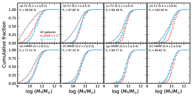
Figure 9: Cumulative fraction of galaxies with $r\leq 20.5$ as a function of stellar mass in four redshift bins: $0.1<z\leq 0.2$, $0.2<z\leq 0.3$, $0.3<z\leq 0.4$, and $0.4<z\leq 0.6$. The upper panels show SHELS/F2 galaxies; the lower panels display HectoMAP galaxies. Black solid lines show the cumulative distribution for all galaxies in each redshift bin. Red dotted lines display quiescent galaxies with ${\rm D}_{n}4000>1.5$ regardless of color. Blue solid lines show galaxies with $(g-r)>1.0$. The numbers denote the recovery fraction for the quiescent population (${\rm D}_{n}4000>1.5$) among the HectoMAP red ($g-r>1.0$) galaxies.

Damjanov et al. (2022a) carry out a similar test based on fainter galaxies ($r>20.5$) with additional $(r-i)>0.5$ selection (their Figure 2). They used the F2 fainter galaxies with $20.5<r<20.75$, the effective F2 survey completeness limit. They demonstrate that the $(r-i)$ color selection for fainter galaxies also recovers ($>98\%$) the quiescent population (i.e., ${\rm D}_{n}4000>1.5$).

5 Comparison between SDSS and HSC Photometry

The HSC-SSP program completely covers the HectoMAP region (Miyazaki et al., 2012; Aihara et al., 2022). Because the HSC-SSP photometry is much deeper than the SDSS, we compare the SDSS with HSC-SSP as a basis for future applications of HectoMAP.

We describe the HSC-SSP photometry in Section 2.1.2. The cross-match of SDSS with HSC-SSP based on R.A. and Decl. identifies HSC counterparts for 92% of the SDSS galaxies brighter than $r=21.3$. HectoMAP galaxies without HSC counterparts are mostly near bright stars that are saturated in the HSC images and thus contaminate or even prevent photometry of the neighboring galaxies. Here, our analysis is based on the cModel magnitudes that are available in both SDSS and HSC-SSP photometry.

Figure 10 compares $g-$ and $r-$band cModel magnitudes from SDSS and HSC. We use only HectoMAP galaxies with spectroscopy for this comparison. The background density maps show the magnitude difference as a function of $g_{cModel,SDSS}$ or $r_{cModel,SDSS}$. The large squares indicate the median difference in each magnitude bin.

The HSC photometry is generally fainter (magnitudes are larger) than the SDSS photometry for bright galaxies with $r<19$. Bosch et al. (2018) and Huang et al. (2018a) argue that the deblending technique applied in hscPipe tends to over-subtract fainter objects and/or extended features surrounding the target galaxies; thus the total flux for bright galaxies is underestimated. In contrast, we suspect that the fainter outskirts of a faint galaxy detected cleanly in the deep HSC images results in a brighter HSC magnitude.

We measure the median systematic difference between SDSS and HSC photometry at $18<g_{cModel}<21$ and $18<r_{cModel}<21$. The typical difference is only $-0.04$ mag in the $g-$band and $-0.05$ mag in the $r-$band. These differences are smaller than the typical uncertainties in the HSC cModel photometry. Huang et al. (2018b) demonstrate that the typical uncertainty in cModel magnitudes for artificially injected galaxies are $\sim 0.15$ mag in both the $g-$ and $r-$ bands. Thus, the magnitude differences between SDSS and HSC-SSP photometry are well within the uncertainties of HSC-SSP photometry.

Figure 11 compares the $(g-r)_{cModel}$ colors from SDSS and HSC. The definition of the symbols is the same as in Figure 10. The color difference is significant for $(g-r)_{cModel}<0.5$. These large differences result from significantly fainter HSC photometry in the $g-$band. Although the $(g-r)_{cModel}$ difference is significant for these blue $(g-r)$ colors, this difference does not affect our analyses because of the red-selection of HectoMAP. The circles in Figure 11 display the median $(g-r)_{cModel}$ difference for galaxies with $18<g_{SDSS,cModel,0}<20$ and $18<g_{HSC,cModel,0}<20$. For these objects, the median $(g-r)_{cModel}$ difference is close to zero over a large color range.

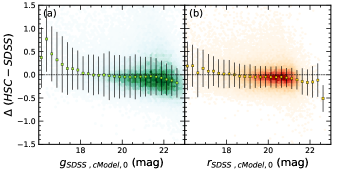
Figure 10: (a) The $g-$band cModel magnitude difference between HSC and SDSS photometry as a function of the SDSS $g-$band magnitude. Large squares and error bars indicate the median difference and the $1\sigma$ standard deviation, respectively. (b) Same as (a), but for $r-$band cModel magnitudes.

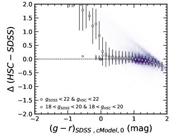
Figure 11: Same as Figure 10, but for $(g-r)_{cModel}$ color.

The spectroscopic survey completeness based on the HSC-SSP photometry (Figure 12) is an interesting aspect of HectoMAP. In fact, the completeness based on HSC photometry is remarkably consistent with that based on SDSS photometry: $\sim 81\%$ at $r_{cModel}<20.5$ and $\sim 65\%$ at $r_{cModel}<21.3$ for $(g-r)_{cModel}>1.0$ galaxies. This consistency is a coincidence. Because of statistical errors in the photometry, particularly in the color, the SDSS and HSC samples are not identical. For example, there are 42,999 spectroscopic sample of galaxies with $r_{SDSS,cModel}<20.5$ and $(g-r)_{SDSS,cModel}>1.0$, but only 80% of these objects have $r_{HSC,cModel}<20.5$ and $(g-r)_{HSC,cModel}>1.0$. Among the missing 8935 galaxies, 74% of them are brighter than $r_{HSC,cModel}=20.5$, but the $(g-r)_{HSC,cModel}$ colors are bluer than the limit. The relatively large uncertainty in the HSC $g-$band photometry underlies in the differences in the samples. Similarly, among 18,744 spectroscopic sample of galaxies with $20.5\leq r_{SDSS,cModel}<21.3$, $(g-r)_{SDSS,cModel}>1.0$ and $(r-i)_{SDSS,cModel}>0.5$, only 70% (12959) of the galaxies satisfy a similar magnitude and color selection based on HSC photometry.

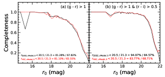
Figure 12: (a)HectoMAP survey completeness for the galaxies with $(g-r)_{cModel}>1.0$ based on the HSC and SDSS photometry. The black solid and red dashed lines show the completeness computed based on SDSS and HSC photometry, respectively. (b) Same as (a), but for galaxies with $(g-r)_{cModel}>1.0$ and $(r-i)_{cModel}>0.5$.

6 Comparison between Photometric and Spectroscopic Redshifts

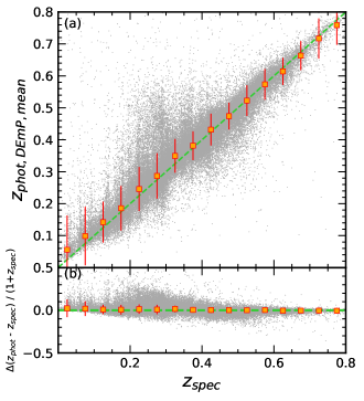
Figure 13: Comparison between HSC DEmP photometric and HectoMAP spectroscopic redshifts. Squares and error bars indicate the median and $1\sigma$ standard deviation as a function of spectroscopic redshift.

The extensive HectoMAP spectroscopy provides a testbed for the updated photometric redshifts from HSC-SSP DR3 (Aihara et al., 2022). In Sohn et al. (2021b), we compared HectoMAP DR1 spectroscopic redshifts with the photometric redshifts based on HSC-SSP DR2 photometry (hereafter DR2 $z_{phot}$). Sohn et al. (2021b) used 17,040 HectoMAP DR1 objects with both spectroscopic and photometric redshifts. They showed that HSC photometric redshifts ($z_{phot}$) are generally consistent with spectroscopic redshifts ($z_{spec}$), but with large scatter. The difference between the $z_{phot}$ and $z_{spec}$ depended significantly on the apparent $i$-band magnitude.

Here we explore the $z_{phot}$ derived with the DEmP template fitting code (Hsieh & Yee, 2014) based on HSC-SSP DR3 (Aihara et al., 2022). Aihara et al. (2022) emphasize changes in the sky subtraction improved the DR3 photometry relative to DR2. These improvements modify the resulting photometric redshifts. We obtain PHOTOZ_MEDIAN, the median value of the photometric redshift probability distribution function, from the DR3 DEmP catalog.

Figure 13 compares $z_{spec}$ and $z_{phot}$ for 88,450 galaxies within the entire HectoMAP region. Figure 13 (a) displays a direct comparison between $z_{spec}$ and $z_{phot}$ and Figure 13 (b) shows the difference between $z_{spec}$ and $z_{phot}$ normalized by $(1+z_{spec})$ as a function of $z_{spec}$. Red squares and error bars indicate the median and $1\sigma$ standard deviation of $z_{phot}$ and $(z_{phot}-z_{spec})/(1+z_{spec})$ as a function of $z_{spec}$.

The typical difference between $z_{spec}$ and $z_{phot}$ in the spectroscopic redshift range $z_{spec}<0.8$ is $0.006\pm 0.050$ (i.e., $1800\pm 15000~{}\rm km~{}s^{-1}$). This difference is comparable with the line-of-sight velocity dispersion of massive galaxy clusters. The typical uncertainties are much larger than the cluster velocity dispersion. The large scatter in $z_{phot}$ measurements thus significantly limits the power of photometric redshifts for studies of galaxy systems and the details of large-scale structure. For example, Figure 18 of Sohn et al. (2021b) shows that the large-scale structure traced by $z_{phot}$ in the HectoMAP DR1 region is almost completely blurred by the scatter in the photometric relative to the spectroscopic redshift.

For further examination of the HSC-SSP DR3 photometric redshifts in comparison with HectoMAP, we revisit three metrics that test the $z_{phot}$ algorithm following Tanaka et al. (2018): the bias, the conventional dispersion, and the loss function. The bias parameter ($\Delta z$) indicates the systematic offset between $z_{phot}$ and $z_{spec}$:

$$\Delta z=(z_{phot}-z_{spec})/(1+z_{spec}).$$ (3)

The conventional dispersion measures the spread in the difference between $z_{phot}$ and $z_{spec}$. We compute the conventional dispersion $\sigma_{conv}$:

$$\sigma_{conv}=1.48\times MAD(z),$$ (4)

where $MAD(z)$ is the median absolute deviation. Finally, we compute the loss function defined by Tanaka et al. (2018):

$$L(\Delta z)=1-{1\over{(1+({{\Delta{z}}\over{\gamma}})^{2})}},$$ (5)

where $\gamma=0.15$ as in Tanaka et al. (2018). This loss function is a continuous version of the outlier fraction that includes both the bias and the dispersion. We follow Tanaka et al. (2018) in taking $\gamma=0.15$ that corresponds to the standard limit $\Delta{z}=0.15$ used for computing the outlier fraction.

Figure 14 (a) shows the three metrics as a function of $i-$band magnitude. Red circles, blue squares, and green crosses indicate $\Delta z$, $\sigma_{conv}$, and the $<L(\Delta z)>$, respectively. The bias remains remains almost constant at $\sim 1600~{}\rm km~{}s^{-1}$ and has little variation with apparent magnitude. Both $\sigma_{conv}$ and $<L(\Delta z)>$ increase slightly at fainter magnitudes.

The solid lines in Figure 14 show the three metrics measured from the earlier HSC-SSP DR1 Tanaka et al. (2018) as a function of magnitude. These metrics are consistent with those for on HSC-SSP DR2 $z_{phot}$ (Figure 19, Sohn et al. (2021b)). Figure 14 shows that the bias and $\sigma_{conv}$ measured from DR2 and DR3 $z_{phot}$ are essentially the same. However, the $<L(\Delta z)>$ measured from DR3 $z_{phot}$ is significantly smaller at $i<21.5$ than it was for DR2. In other words, the DR3 photometric redshifts $z_{phot}$ are a significant improvement over DR2. The revised sky subtraction procedures (Aihara et al., 2022) are probably responsible at least in part for this improvement.

Figure 14 (b) and (c) display the same metrics as a function of $z_{spec}$ and $z_{phot}$, respectively (See Figure 19 of Sohn et al. (2021b) for the DR2 comparison). All three metrics show similar trends with either $z_{spec}$ or $z_{phot}$. The bias decreases slightly as a function of spectroscopic redshift. The value of the bias is zero at $z\sim 0.4$; the bias is positive (negative) at lower (higher) redshift. This trend differs from the bias based on DR2 $z_{phot}$, where the bias is positive over the entire redshift range we explore (Sohn et al., 2021b). The $\sigma_{conv}$ changes little as a function of redshift as for DR2 photometric redshifts (Sohn et al., 2021b).

Interestingly, the loss function shows a distinctive behavior compared to that of the DR2 $z_{phot}$ (Sohn et al., 2021b). For DR2 $z_{phot}$, the loss function is larger than 0.1 at $z<0.1$ and remains constant at $\sim 0.06$ at $z>0.1$. In contrast, the DR3 $z_{phot}$ loss function is generally below the DR2 result at every redshift. There are significant fluctuations in the loss function in the range $0.2<z<0.4$ (Figure 13) both as a function of $z_{spec}$ and $z_{phot}$. This effect probably results from the larger number of well-sampled many galaxy systems in this redshift range. Naturally, larger photometric uncertainties in these crowded fields can affect the $z_{phot}$ measurements.

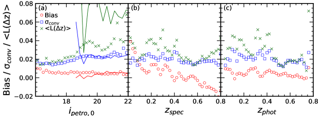
Figure 14: The bias ($\Delta z$, red circles), the conventional dispersion ($\sigma_{conv}$, blue squares), and the loss function ($<L(\Delta z)>$, green crosses) as a function of (a) SDSS $i-$band magnitude, (b) $z_{spec}$ and (c) $z_{phot}$. The solid lines in (a) show the distribution of the three metrics derived based on HSC-SSP PDR1 $z_{phot}$ (Tanaka et al., 2018).

7 Applications of HectoMAP to Clusters and the Cosmic Web

The area of HectoMAP (54.64 deg²) combined with its density ($\sim 1800$ galaxies deg^-2) and depth enable exploration of a wide range of scientific issues. We summarize some of the existing projects enabled by the survey and we preview a few of its future applications.

The high density of the red-selected HectoMAP survey makes it a foundation for the study of clusters of galaxies in the redshift range $0.2<z<0.6$ (Sohn et al., 2018b, a, 2021a). There are 104 photometrically selected redMaPPer clusters in the HectoMAP region (Rykoff et al., 2016; Sohn et al., 2018b). More than 90% of redMaPPer clusters include 10 or more HectoMAP spectroscopic members, a basis for evaluating the redMaPPer membership probability and for defining a spectroscopic richness.

Sohn et al. (2021a) identify galaxy clusters based purely on spectroscopy by applying a friends-of-friends algorithm. There are 346 galaxy overdensities with 10 or more spectroscopic members. Even among relatively dense systems in this friends-of-friends catalog, $\sim 70\%$ have no redMaPPer counterpart suggesting that the solely photometric catalog may be incomplete.

HectoMAP is the first survey that traces cluster infall regions, the link between clusters and the cosmic web. HectoMAP traces the infall regions for clusters in the mass range $M_{200}>5\times 10^{13}~{}{\rm M}_{\odot}$ for the redshift range $0.2<z<0.6$. Pizzardo et al. (2022) use a technique developed by De Boni et al. (2016) to measure the growth rate of clusters directly over the HectoMAP redshift range. This technique, which depends on observations of the infall region, yields a growth rate consistent with predictions of simulations.

One of the special strengths of HectoMAP is the combination of the dense spectroscopy with the deep HSC-SSP imaging. This combination enables a range of projects that combine two of the most powerful cosmological tools, lensing and redshift surveys.

Shapes for weak lensing sources have not yet been released for the entire HectoMAP region. Eventually, these data will enable weak lensing studies ranging from examining of the masses of quiescent galaxies and their evolution to tracing the matter distribution in the cosmic web by comparing the foreground galaxy distribution with the weak lensing map (e.g., Utsumi et al., 2016). For the friends-of-friends clusters, weak lensing adds another mass proxy.

Jaelani et al. (2020) identify 23 candidate strong lensing systems in the HectoMAP region from HSC-SSP. Many of these systems have redshifts beyond the HectoMAP effective limit, but 8 of these systems match friends-of-friends systems. Figure 15 shows HSC images of the 8 strong lensing systems. The lower right panel of Figure 15 shows the redshift distribution of the strong lensing systems compared with the HectoMAP redshift distribution. In general, the more abundant, higher redshift systems have more obvious substructures frequently with multiple BCGs. Although this sample is small, it promises probes of cluster evolution, the relation between clusters and their BCGs, and the underlying cluster geometry that produces a strong lensing system.

HectoMAP densely samples the filaments and walls in the cosmic web that delineate the void regions. Hwang et al. (2016) identify the underdense void regions in HectoMAP at $z>0.2$. They show that the observed void properties including size and volume are in agreement with predicted void properties based on numerical simulations. Geller et al. (2010) used the SHELS survey and DLS photometry to pioneer the direct comparison between structure in a redshift survey and a weak lensing map. A similar comparison based on HectoMAP and HSC-SSP will probe the relative distribution of light-emitting and dark matter on large scales.

HectoMAP is a testbed of approaches to understanding the mass distribution in the universe and its evolution. Future large, deeper surveys including DESI (Zhou et al., 2022), MOONS (Taylor et al., 2018), WEAVE (Dalton et al., 2012), 4MOST (Richard et al., 2019), Subaru/Prime Focus Spectrograph (PFS, Takada et al., 2014; Greene et al., 2022) survey will enhance these approaches and develop techniques taking advantage of the large extent and depth of these surveys.

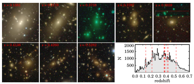
Figure 15: HSC images of 8 strong lensing clusters identified by both Jaelani et al. (2020) and Sohn et al. (2021a). The lower inset shows the redshift distribution of HectoMAP galaxies (black histogram) and the redshifts of the strong lensing clusters (red vertical lines).

8 CONCLUSION

HectoMAP is a dense redshift survey with a median redshift of $z=0.345$. It densely covers 54.64 square degrees in a 1.5 degree wide strip across the northern sky centered at a declination of 43.25^∘. The survey is dense ($\sim 1800$ galaxies deg^-2) and focused on the quiescent galaxy population. The survey includes 95,403 galaxies: among these galaxies, 60,237 are quiescent.

On average there were 9 visits to each position in the survey. Thus the overall completeness is high and uniform. The completeness is $\sim 81\%$ and $\sim 72\%$ for galaxies with $r<20.5$ and $(g-r)>1.0$, and with $20.5<r<21.3$, $(g-r)>1.0$, and $(r-i)>0.5$, respectively.

Sohn et al. (2021b) published a first data release covering 8.7 deg² of the survey area. They show individual spectra and substantiate the choice of a limiting cross-correlation value to identify objects with reliable redshifts. They also make a detailed comparison between HectoMAP and SDSS/BOSS redshifts. The small offset of $26~{}\rm km~{}s^{-1}$ and $46~{}\rm km~{}s^{-1}$ persists for the larger sample. These small offsets are comparable with the redshift errors and do not affect any of the analysis carried out so far with HectoMAP data.

In addition to the 88294 MMT/Hectospec redshifts provided here, we include the spectral diagnostic (${\rm D}_{n}4000$) and stellar masses for 88165 galaxies. We highlight the distributions of these quantities in the HectoMAP survey data. As expected for a red-selected survey, the majority of the objects (63%) are quiescent. The distribution of stellar masses is skewed toward large stellar mass reflecting this selection.

As Damjanov et al. (2022a) emphasize, HectoMAP provides one of the largest, complete, mass-limited samples of quiescent galaxies covering the redshift range $0.2<z<0.6$. The sample includes 30,231 galaxies. Damjanov et al. (2022a) use the sample to trace the size-mass relation of the quiescent population and to track the growth of various subpopulations with cosmic time.

One of the distinctive characteristics of HectoMAP is the full HSC-SSP coverage of the entire region. Observations for HectoMAP occurred over a 10 year period and thus the photometric basis was limited to the SDSS. We compare the SDSS DR16 photometry with the HSC-SSP photometry and show that the typical differences between the SDSS and HSC-SSP $g-$ and $r-$ band photometry are small compared with the photometric error. We also show that for red galaxies that are the bulk of the HectoMAP sample, the $(g-r)$ colors also agree; the difference for blue objects is significant. Remarkably, the completeness of HectoMAP is similar to both the SDSS and HSC-SSP magnitude limits, but the underlying samples in the two cases differ as a result of photometric error.

The extensive HectoMAP spectroscopic redshifts provide a platform for testing HSC-SSP photometric redshifts. We revisit the comparison between $z_{phot}$ and $z_{spec}$ reported in Sohn et al. (2021b). Here we used the updated HSC-SSP DR3 $z_{phot}$. The DR3 $z_{phot}$ measurements are a significant improvement over the earlier DR2 photometric redshifts. In general, $z_{phot}$ agrees well with $z_{spec}$, but the scatter remains large ($\sim 1800\pm 15,000~{}\rm km~{}s^{-1}$) compared with the typical velocity dispersions of galaxy systems.

Finally we highlight the particular power of HectoMAP for exploring clusters of galaxies. The survey contains an independently identified set of strong lensing clusters in the redshift range $0.2<z<0.6$. When full HSC-SSP shapes are available, weak lensing mass profiles combined with extensive on the strong lensing systems will elucidate evolutionary issues and the role of substructure along the line-of-sight in enhancing the lensing cross-section. More generally, HectoMAP covers a redshift range where clusters of galaxies accrete roughly half of their mass (e.g., Fakhouri et al., 2010; Sohn et al., 2022). Pizzardo et al. (2022) measure the accretions rate for HectoMAP clusters and show that it agrees with predictions. Taken together these explorations of cluster growth and structure will inform the design of future larger, deeper dense surveys.

At the moment, HectoMAP has some distinctive features in the universe of redshift surveys; it is dense and red-selected. For example, in contrast with the 1800 galaxy deg^-2 density of HectoMAP, the DESI bright galaxy sample (Ruiz-Macias et al., 2021), though it will be much larger, reaches a limiting $r<19.5$ with only 864 galaxies deg^-2 and the BGS faint sample covers the range $19.5<r<20.175$ with a density of 533 galaxies deg^-2. HectoMAP is a platform for investigating issues including the nature and evolution of the quiescent population, the growth of clusters of galaxies, and the way galaxies trace the matter distribution in the universe. The HectoMAP data and analyses will contribute to informing the design and goals of ongoing major surveys.

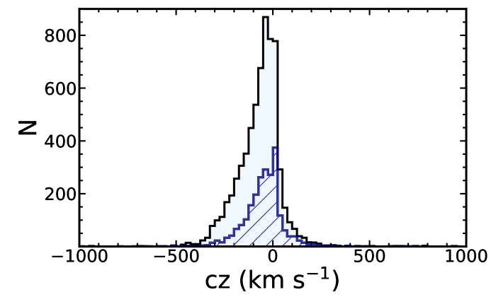
Figure 16: Radial velocity distribution of stars with HectoMAP spectroscopy. The hatched histogram shows the distribution for stars identified as extended sources in the SDSS photometry alone.

Table 4: Radial Velocities for Stars in HectoMAP

SDSS Object ID	R.A.	Decl.	RVa	$r_{petro,0}$	Flagb
	(deg)	(deg)	($\rm km~{}s^{-1}$)	(mag)
1237661360226500918	208.899206	43.773073	$108.82\pm 122.02$	$21.13\pm 0.13$	Extended
1237661360226500771	208.808559	43.794296	$-36.48\pm 29.98$	$20.49\pm 0.07$	Point
1237661360763633780	209.840059	43.983869	$-40.41\pm 6.18$	$17.29\pm 0.00$	Point
1237661433241862442	208.388763	43.964662	$-262.36\pm 28.11$	$20.90\pm 0.06$	Point
1237661433242058831	208.999039	43.988056	$-19.59\pm 16.66$	$21.75\pm 1.40$	Point
1237661433242190333	209.325341	43.897316	$18.45\pm 11.00$	$21.27\pm 0.23$	Point
1237661433242189895	209.230960	43.803751	$-78.14\pm 7.72$	$18.85\pm 0.01$	Point
1237661849863651845	200.241813	43.048129	$-76.82\pm 13.45$	$20.65\pm 0.07$	Point
1237661849863585864	200.125410	43.083937	$1275.91\pm 100.00$	$12.29\pm 0.01$	Extended

References

- Ahumada et al. (2020) Ahumada, R., Prieto, C. A., Almeida, A., et al. 2020, ApJS, 249, 3, doi: 10.3847/1538-4365/ab929e
- Aihara et al. (2022) Aihara, H., AlSayyad, Y., Ando, M., et al. 2022, PASJ, 74, 247, doi: 10.1093/pasj/psab122
- Arnouts et al. (1999) Arnouts, S., Cristiani, S., Moscardini, L., et al. 1999, MNRAS, 310, 540, doi: 10.1046/j.1365-8711.1999.02978.x
- Astropy Collaboration et al. (2013) Astropy Collaboration, Robitaille, T. P., Tollerud, E. J., et al. 2013, A&A, 558, A33, doi: 10.1051/0004-6361/201322068
- Astropy Collaboration et al. (2018) Astropy Collaboration, Price-Whelan, A. M., Sipőcz, B. M., et al. 2018, AJ, 156, 123, doi: 10.3847/1538-3881/aabc4f
- Balogh et al. (1999) Balogh, M. L., Morris, S. L., Yee, H. K. C., Carlberg, R. G., & Ellingson, E. 1999, ApJ, 527, 54, doi: 10.1086/308056
- Blanton & Moustakas (2009) Blanton, M. R., & Moustakas, J. 2009, ARA&A, 47, 159, doi: 10.1146/annurev-astro-082708-101734
- Blanton & Roweis (2007) Blanton, M. R., & Roweis, S. 2007, AJ, 133, 734, doi: 10.1086/510127
- Bosch et al. (2018) Bosch, J., Armstrong, R., Bickerton, S., et al. 2018, PASJ, 70, S5, doi: 10.1093/pasj/psx080
- Bruzual & Charlot (2003) Bruzual, G., & Charlot, S. 2003, MNRAS, 344, 1000, doi: 10.1046/j.1365-8711.2003.06897.x
- Calzetti et al. (2000) Calzetti, D., Armus, L., Bohlin, R. C., et al. 2000, ApJ, 533, 682, doi: 10.1086/308692
- Chabrier (2003) Chabrier, G. 2003, PASP, 115, 763, doi: 10.1086/376392
- Conroy et al. (2009) Conroy, C., Gunn, J. E., & White, M. 2009, ApJ, 699, 486, doi: 10.1088/0004-637X/699/1/486
- Dalton et al. (2012) Dalton, G., Trager, S. C., Abrams, D. C., et al. 2012, in Society of Photo-Optical Instrumentation Engineers (SPIE) Conference Series, Vol. 8446, Ground-based and Airborne Instrumentation for Astronomy IV, ed. I. S. McLean, S. K. Ramsay, & H. Takami, 84460P, doi: 10.1117/12.925950
- Damjanov et al. (2022a) Damjanov, I., Sohn, J., Geller, M. J., Utsumi, Y., & Dell’Antonio, I. 2022a, arXiv e-prints, arXiv:2210.01129. https://arxiv.org/abs/2210.01129
- Damjanov et al. (2022b) Damjanov, I., Sohn, J., Utsumi, Y., Geller, M. J., & Dell’Antonio, I. 2022b, ApJ, 929, 61, doi: 10.3847/1538-4357/ac54bd
- Damjanov et al. (2018) Damjanov, I., Zahid, H. J., Geller, M. J., Fabricant, D. G., & Hwang, H. S. 2018, ApJS, 234, 21, doi: 10.3847/1538-4365/aaa01c
- Davies et al. (2018) Davies, L. J. M., Robotham, A. S. G., Driver, S. P., et al. 2018, MNRAS, 480, 768, doi: 10.1093/mnras/sty1553
- Davis et al. (1982) Davis, M., Huchra, J., Latham, D. W., & Tonry, J. 1982, ApJ, 253, 423, doi: 10.1086/159646
- De Boni et al. (2016) De Boni, C., Serra, A. L., Diaferio, A., Giocoli, C., & Baldi, M. 2016, ApJ, 818, 188, doi: 10.3847/0004-637X/818/2/188
- Fabricant et al. (2005) Fabricant, D., Fata, R., Roll, J., et al. 2005, PASP, 117, 1411, doi: 10.1086/497385
- Fakhouri et al. (2010) Fakhouri, O., Ma, C.-P., & Boylan-Kolchin, M. 2010, MNRAS, 406, 2267, doi: 10.1111/j.1365-2966.2010.16859.x
- Geller & Huchra (1989) Geller, M. J., & Huchra, J. P. 1989, Science, 246, 897, doi: 10.1126/science.246.4932.897
- Geller et al. (2016) Geller, M. J., Hwang, H. S., Dell’Antonio, I. P., et al. 2016, ApJS, 224, 11, doi: 10.3847/0067-0049/224/1/11
- Geller et al. (2014) Geller, M. J., Hwang, H. S., Fabricant, D. G., et al. 2014, ApJS, 213, 35, doi: 10.1088/0067-0049/213/2/35
- Geller et al. (2010) Geller, M. J., Kurtz, M. J., Dell’Antonio, I. P., Ramella, M., & Fabricant, D. G. 2010, ApJ, 709, 832, doi: 10.1088/0004-637X/709/2/832
- Greene et al. (2022) Greene, J., Bezanson, R., Ouchi, M., Silverman, J., & the PFS Galaxy Evolution Working Group. 2022, arXiv e-prints, arXiv:2206.14908. https://arxiv.org/abs/2206.14908
- Hahn et al. (2022) Hahn, C., Wilson, M. J., Ruiz-Macias, O., et al. 2022, arXiv e-prints, arXiv:2208.08512. https://arxiv.org/abs/2208.08512
- Hamadouche et al. (2022) Hamadouche, M. L., Carnall, A. C., McLure, R. J., et al. 2022, MNRAS, 512, 1262, doi: 10.1093/mnras/stac535
- Hsieh & Yee (2014) Hsieh, B. C., & Yee, H. K. C. 2014, ApJ, 792, 102, doi: 10.1088/0004-637X/792/2/102
- Huang et al. (2018a) Huang, S., Leauthaud, A., Greene, J. E., et al. 2018a, MNRAS, 475, 3348, doi: 10.1093/mnras/stx3200
- Huang et al. (2018b) Huang, S., Leauthaud, A., Murata, R., et al. 2018b, PASJ, 70, S6, doi: 10.1093/pasj/psx126
- Hwang et al. (2016) Hwang, H. S., Geller, M. J., Park, C., et al. 2016, ApJ, 818, 173, doi: 10.3847/0004-637X/818/2/173
- Ilbert et al. (2006) Ilbert, O., Arnouts, S., McCracken, H. J., et al. 2006, A&A, 457, 841, doi: 10.1051/0004-6361:20065138
- Jaelani et al. (2020) Jaelani, A. T., More, A., Oguri, M., et al. 2020, MNRAS, 495, 1291, doi: 10.1093/mnras/staa1062
- Kauffmann et al. (2004) Kauffmann, G., White, S. D. M., Heckman, T. M., et al. 2004, MNRAS, 353, 713, doi: 10.1111/j.1365-2966.2004.08117.x
- Kauffmann et al. (2003) Kauffmann, G., Heckman, T. M., White, S. D. M., et al. 2003, MNRAS, 341, 33, doi: 10.1046/j.1365-8711.2003.06291.x
- Kochanek et al. (2012) Kochanek, C. S., Eisenstein, D. J., Cool, R. J., et al. 2012, ApJS, 200, 8, doi: 10.1088/0067-0049/200/1/8
- Kurtz et al. (2012) Kurtz, M. J., Geller, M. J., Utsumi, Y., et al. 2012, ApJ, 750, 168, doi: 10.1088/0004-637X/750/2/168
- Kurtz & Mink (1998) Kurtz, M. J., & Mink, D. J. 1998, PASP, 110, 934, doi: 10.1086/316207
- Lazo et al. (2018) Lazo, B., Zahid, H. J., Sohn, J., & Geller, M. J. 2018, Research Notes of the American Astronomical Society, 2, 234, doi: 10.3847/2515-5172/aaf8b1
- Liske et al. (2015) Liske, J., Baldry, I. K., Driver, S. P., et al. 2015, MNRAS, 452, 2087, doi: 10.1093/mnras/stv1436
- Maiolino et al. (2020) Maiolino, R., Cirasuolo, M., Afonso, J., et al. 2020, The Messenger, 180, 24, doi: 10.18727/0722-6691/5197
- Miyazaki et al. (2012) Miyazaki, S., Komiyama, Y., Nakaya, H., et al. 2012, in Society of Photo-Optical Instrumentation Engineers (SPIE) Conference Series, Vol. 8446, Ground-based and Airborne Instrumentation for Astronomy IV, ed. I. S. McLean, S. K. Ramsay, & H. Takami, 84460Z, doi: 10.1117/12.926844
- Petrosian (1976) Petrosian, V. 1976, ApJ, 210, L53, doi: 10.1086/182301
- Pizzardo et al. (2022) Pizzardo, M., Sohn, J., Geller, M. J., Diaferio, A., & Rines, K. 2022, ApJ, 927, 26, doi: 10.3847/1538-4357/ac5029
- Richard et al. (2019) Richard, J., Kneib, J. P., Blake, C., et al. 2019, The Messenger, 175, 50, doi: 10.18727/0722-6691/5127
- Rines et al. (2016) Rines, K. J., Geller, M. J., Diaferio, A., & Hwang, H. S. 2016, ApJ, 819, 63, doi: 10.3847/0004-637X/819/1/63
- Robotham et al. (2010) Robotham, A., Driver, S. P., Norberg, P., et al. 2010, PASA, 27, 76, doi: 10.1071/AS09053
- Ruiz-Macias et al. (2021) Ruiz-Macias, O., Zarrouk, P., Cole, S., et al. 2021, MNRAS, 502, 4328, doi: 10.1093/mnras/stab292
- Rykoff et al. (2016) Rykoff, E. S., Rozo, E., Hollowood, D., et al. 2016, ApJS, 224, 1, doi: 10.3847/0067-0049/224/1/1
- Shectman et al. (1996) Shectman, S. A., Landy, S. D., Oemler, A., et al. 1996, ApJ, 470, 172, doi: 10.1086/177858
- Sohn et al. (2018a) Sohn, J., Chon, G., Böhringer, H., et al. 2018a, ApJ, 855, 100, doi: 10.3847/1538-4357/aaac7a
- Sohn et al. (2021a) Sohn, J., Geller, M. J., Hwang, H. S., et al. 2021a, ApJ, 923, 143, doi: 10.3847/1538-4357/ac29c3
- Sohn et al. (2021b) —. 2021b, ApJ, 909, 129, doi: 10.3847/1538-4357/abd9be
- Sohn et al. (2018b) Sohn, J., Geller, M. J., Rines, K. J., et al. 2018b, ApJ, 856, 172, doi: 10.3847/1538-4357/aab20b
- Sohn et al. (2022) Sohn, J., Geller, M. J., Vogelsberger, M., & Borrow, J. 2022, ApJ, 938, 3, doi: 10.3847/1538-4357/ac8f23
- Sohn et al. (2017a) Sohn, J., Geller, M. J., Zahid, H. J., et al. 2017a, ApJS, 229, 20, doi: 10.3847/1538-4365/aa653e
- Sohn et al. (2017b) Sohn, J., Zahid, H. J., & Geller, M. J. 2017b, ApJ, 845, 73, doi: 10.3847/1538-4357/aa7de3
- Strauss et al. (2002) Strauss, M. A., Weinberg, D. H., Lupton, R. H., et al. 2002, AJ, 124, 1810, doi: 10.1086/342343
- Takada et al. (2014) Takada, M., Ellis, R. S., Chiba, M., et al. 2014, PASJ, 66, R1, doi: 10.1093/pasj/pst019
- Tanaka et al. (2018) Tanaka, M., Coupon, J., Hsieh, B.-C., et al. 2018, PASJ, 70, S9, doi: 10.1093/pasj/psx077
- Taylor et al. (2018) Taylor, W., Cirasuolo, M., Afonso, J., et al. 2018, in Society of Photo-Optical Instrumentation Engineers (SPIE) Conference Series, Vol. 10702, Ground-based and Airborne Instrumentation for Astronomy VII, ed. C. J. Evans, L. Simard, & H. Takami, 107021G, doi: 10.1117/12.2313403
- Utsumi et al. (2016) Utsumi, Y., Geller, M. J., Dell’Antonio, I. P., et al. 2016, ApJ, 833, 156, doi: 10.3847/1538-4357/833/2/156
- Vergani et al. (2008) Vergani, D., Scodeggio, M., Pozzetti, L., et al. 2008, A&A, 487, 89, doi: 10.1051/0004-6361:20077910
- Wittman et al. (2006) Wittman, D., Dell’Antonio, I. P., Hughes, J. P., et al. 2006, ApJ, 643, 128, doi: 10.1086/502621
- Woods et al. (2010) Woods, D. F., Geller, M. J., Kurtz, M. J., et al. 2010, AJ, 139, 1857, doi: 10.1088/0004-6256/139/5/1857
- Zahid et al. (2019) Zahid, H. J., Geller, M. J., Damjanov, I., & Sohn, J. 2019, ApJ, 878, 158, doi: 10.3847/1538-4357/ab21b9
- Zahid et al. (2016) Zahid, H. J., Geller, M. J., Fabricant, D. G., & Hwang, H. S. 2016, ApJ, 832, 203, doi: 10.3847/0004-637X/832/2/203
- Zhou et al. (2022) Zhou, R., Dey, B., Newman, J. A., et al. 2022, arXiv e-prints, arXiv:2208.08515. https://arxiv.org/abs/2208.08515