Fiber Organization has Little Effect on Electrical Activation Patterns during Focal Arrhythmias in the Left Atrium

Abstract

Over the past two decades there has been a steady trend towards the development of realistic models of cardiac conduction with increasing levels of detail. However, making models more realistic complicates their personalization and use in clinical practice due to limited availability of tissue and cellular scale data. One such limitation is obtaining information about myocardial fiber organization in the clinical setting. In this study, we investigated a chimeric model of the left atrium utilizing clinically derived patient-specific atrial geometry and a realistic, yet foreign for a given patient fiber organization. We discovered that even significant variability of fiber organization had a relatively small effect on the spatio-temporal activation pattern during regular pacing. For a given pacing site, the activation maps were very similar across all fiber organizations tested.

I Introduction

Over the past two decades, there has been steady progress towards the development of realistic electrophysiological models [1, 2, 3] of cardiac propagation with detailed description of gross cardiac anatomy [4, 5, 6], myocardial fiber organization [7, 8], and ionic currents involved in the generation of cardiac action potentials [9, 10, 11]. At the same time, the focus of modeling studies has been gradually shifting from the investigation of fundamental mechanisms of cardiac arrhythmias [12, 13, 14, 15, 16] towards clinical applications [17, 18, 19]. The range of applications that are actively been explored includes screening anti-arrhythmic [20, 21] and pro-arrhythmic [22, 23] drugs, optimizing anti-tachycardia [24] and anti-fibrillation [25, 26] pacing protocols, and aiding arrhythmia ablation procedures [27, 28], among others.

One of the key obstacles towards the development of constructing patient-specific models is not only speed in simulations [11] but adequate quantification, verification and information for such models [29, 30]. Detailed models have a very high-dimensional parameter space; moreover, most of the parameters cannot be measured on an individual basis and need to be postulated based on some generic values or recomputed libraries [31, 32]. In this study, we investigate the problem of incorporating realistic myocardial fiber organization into an atrial conduction model, and their effect in the electrical propagation.

The velocity of action potential propagation along fibers is typically 2-3 times faster than across fibers [33], which makes fiber organization one of the key factors determining activation patterns in cardiac tissue [34, 35]. Unlike atrial geometry, which can be readily obtained in a clinical setting via electroanatomical mapping [36] or from clinical imaging, fiber organization cannot be obtained with a sufficient level of detail in live tissue [37]. To date, the best available resource for real patient fiber data is an ex-vivo Diffusion Tensor Magnetic Resonance Imaging (DT-MRI) fiber database [38, 39], which required about 50 hours to scan each atrium [38].

The focus of our study is on modeling the left atrium, which is known to harbor the most common sources of atrial fibrillation and thus is particularly important with regard to potential clinical applications. Here we explore 3D chimeric models of the left atrium informed by a patient-specific DT-MRI-derived geometry and various fiber direction patterns adopted from the DT-MRI fiber database. Specifically, we investigate models with identical atrial geometry but with different fiber organization. By assuming one of these models as the ground-truth, we assess the capability of the others for predicting activation patterns produced by focal excitation sources located in different areas of the left atrium.

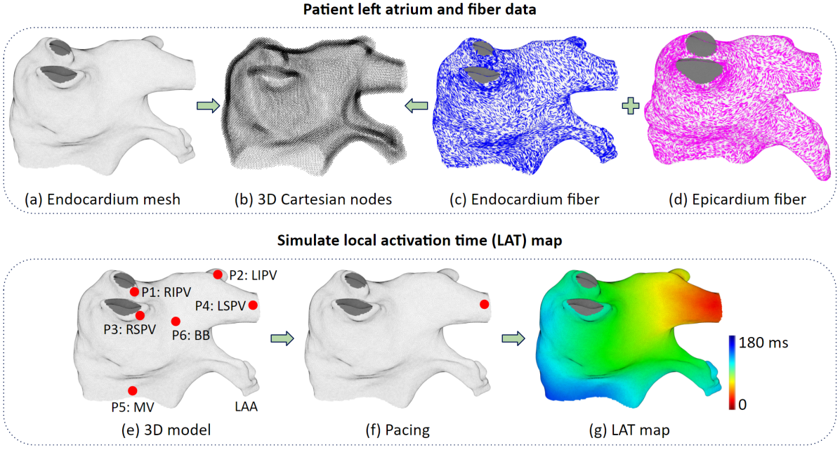
Figure 1: Generation of surrogate activation maps in the ground-truth and chimeric models. (a) The endocardial mesh of left atrium 1 ($M_{endo1}$). (b) $M_{endo1}$ transformed into 3D Cartesian nodes to be used for modeling action potential propagation. (c, d) Endocardial and epicardial fiber organizations ($F_{endo1}$, $F_{endo2}$, …, $F_{endo7}$ and $F_{epi1}$, $F_{epi2}$, …, $F_{epi7}$) registered onto the nodes. (e) Locations of the pacing sites. (f, g) Example of a local activation time map produced from a pacing site. (RIPV: Right Inferior Pulmonary Vein, LIPV: Left Inferior Pulmonary Vein, RSPV: Right Superior Pulmonary Vein, LSPV: Left Superior Pulmonary Vein, MV: Mitral Valve, BB: Bachmann’s Bundle, LAA: Left Atrial Appendage.)

The rest of this paper is organized as follows: We first describe the procedure for constructing in-silico heart models utilizing clinically derived patient-specific left atrial geometry and realistic fiber organization. We then show our results of heart models with different fiber organization in terms of Local Activation Time (LAT) and spatial activation patterns. In the discussion, we validate our models and explain the results in terms of a cancellation effect across the atrium. Finally, we describe the potential application to fiber-independent patient-specific heart models, list the limitations of our work, and summarize the main contributions.

II Method

II-A Ground-Truth and Chimeric Models

To generate ground-truth and chimeric models of action potential propagation in the left atrium, we used a DT-MRI fiber database [39]. It contains data sets from seven left atria, which are denoted as $LA_{1}$, $LA_{2}$, …, $LA_{7}$. The different fiber organizations are denoted as $F_{1}$, $F_{2}$, …, $F_{7}$, each can be subdivided into endocardium and epicardium fiber organizations, and are denoted as $F_{endo1}$, $F_{endo2}$…, $F_{endo7}$ and $F_{epi1}$, $F_{epi2}$, …, $F_{epi7}$, respectively. Endocardial and epicardial triangular meshes are denoted as $M_{endo1}$, $M_{endo2}$, …, $M_{endo7}$ and $M_{epi1}$, $M_{epi2}$, …, $M_{epi7}$, respectively.

We used $M_{endo1}$ and $F_{1}$ to generate ground-truth models of action potential propagation and surrogate clinical activation maps. $M_{endo1}$ was chosen because $LA_{1}$’s fiber organization was found to be the optimal one, giving the least LAT errors among the seven left atria for bi-layer model atrial fibrillation simulations [39]. We used $M_{endo1}$ and $F_{2}$, $F_{3}$, …, $F_{7}$ to generate six chimeric models. We called them chimeric models because foreign fibers were registered onto the left atrium.

Fig. 1 illustrates the generation of all models. The process involves generation of 3D Cartesian nodes around $M_{endo1}$, mapping of the respective fiber organizations onto the nodes, simulation of action potential propagation from stimuli in different locations, and generation of surrogate clinical activation maps. The latter were then used for evaluation of chimeric model performance in predicting activation patterns across different fiber patterns.

II-B Atrium mesh and fiber processing

Triangular mesh $M_{endo1}$ has 63,112 vertices, 125,501 faces, and its average triangle edge length is 0.67 mm. The seven fiber organizations are registered onto $M_{endo1}$, resulting in seven different models (one ground-truth model and six chimeric models). This procedure requires morphing other meshes and fibers onto $M_{endo1}$. Details in Appendix A.

The next step is to create 3D Cartesian nodes wrapped around $M_{endo1}$, as shown in Fig. 2(b). First, a cubic space that contains $M_{endo1}$ is filled with equally spaced nodes (1 mm spacing), then nodes that are further than a distance threshold from the $M_{endo1}$ surface are removed. Here, the left atrium tissue thickness is set at 2 mm, which is in the range of clinically observed values [40, 41], and the total number of Cartesian nodes is 60,691. The endocardium and epicardium layers split the tissue thickness in half, each having a thickness of 1 mm. The spatial resolution is chosen to be adequate (refer to Appendix C) for accurate simulation without being computationally demanding.

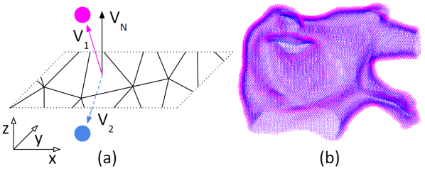
Figure 2: Labeling of endocardial and epicardial nodes. (a) $V_{1}$ and $V_{2}$ are vectors pointing from the nearest triangle center to the respective node. $V_{N}$ is the surface normal vector. Because the angle between $V_{1}$ and $V_{N}$ is less than 90°, the magenta node was labeled as an epicardial node; If the angle is larger than 90°, the blue node was labeled as an endocardial node. If the angle is equal to 90°, then randomly assign it to endocardial or epicardial node. (b) All left atrial nodes labeled as epicardial (magenta) or endocardial (blue) nodes.

Each node of the grid was attributed to either the epicardial or endocardial layer, based on its location with respect to $M_{endo1}$. The appropriate layer was determined by the angle between the vector pointing to the respective node from the center of the closest triangle and the normal vector of this triangle. Note that although there are two normal directions (opposite to each other) for a triangle, we can easily determine which points out from the mesh: it is a property of a triangular mesh that the three vertices of a triangle are in a particular sequence, and the outward normal vector thus can be found according to the sequence and the right-hand-rule. Fig. 2 shows the labeled epicardial and endocardial nodes. Then the endocardial and epicardial fibers were assigned to these nodes via minimum distance mapping.

II-C Heart model equations

To simulate action potentials, we used the Mitchell-Schaeffer model [42], as shown in (1). This model was chosen because its simplicity makes it efficient in 3D numerical simulations, and the parameters provide direct insight into changes in electrophysiological behavior. It models the inward current caused by sodium and calcium ion channels, outward current caused by potassium channels, and external stimulus current.

$$\begin{split}\frac{du}{dt}&=\frac{hu^{2}(1-u)}{\tau_{in}}-\frac{u}{\tau_{out}}+J_{stimulus}+\bigtriangledown\cdot(D\bigtriangledown u)\\ \frac{dh}{dt}&=\left\{\begin{matrix}\ \frac{1-h}{\tau_{open}}\ \text{if}\ u<u_{gate}\\ \ \frac{-h}{\tau_{close}}\ \text{if}\ u\geq u_{gate}\end{matrix}\right.\end{split}$$ (1)

The variables are as follows:

• $u$ is the transmembrane voltage and $h$ is an inactivation gating variable for the inward current.

• $\tau_{in},\tau_{close},\tau_{out},\tau_{open}$ and $u_{gate}$ are parameters that control the action potential shape.

• $J_{stimulus}$ is an external current applied locally as impulses to initiate action potential. We specified this impulse to have 1 ms duration and a magnitude of 20.

• $\bigtriangledown\cdot(D\bigtriangledown u)$ is the diffusion term, responsible for action potential propagation.

For each node, fiber anisotropy is introduced via a $3\times 3$ diffusion tensor $D$ according to (2),

$$D =d\left(rI+\left(1-r\right)ff^{\top}\right)$$ (2)

$$r =\frac{d_{T}}{d_{L}}=\left(\frac{CV_{T}}{CV_{L}}\right)^{2}$$ (3)

where $d$ is the diffusion coefficient. $r$ is the anisotropy ratio, a ratio of fiber’s transverse to longitudinal diffusion coefficients, or the ratio of transverse to longitudinal conduction velocities squared. $I$ is the identity matrix, and $f$ is a $3\times 1$ unit vector pointing along the fiber direction [43].

The differential equations (1) were solved using the explicit Euler method on the Cartesian nodes. We followed [44] that assumed no-flux boundary conditions and used a 19-node stencil. The time step is 0.01 ms and the spatial resolution is 1 mm. Such resolution is adequate, refer to Appendix C for details. The parameters are given nominal values as shown in Table I [45, 46]. With this setting, the Conduction Velocity (CV) will be around 0.69 m/s, which is a typical value for the atrium. The model is implemented in MATLAB (MathWorks, Natick, Massachusetts, United States) and accelerated with GPU computing using CUDA kernels (Nvidia, Santa Clara, California, United States).

Table I: Nominal parameter values

$\tau_{in}$	$\tau_{out}$	$\tau_{open}$	$\tau_{close}$	$u_{gate}$	$r$	$d$
0.3 ms	6 ms	120 ms	150 ms	0.13 mV	0.2	1

III Results

III-A Fibers vary significantly across different atria

To compare fiber organization in different models of the left atrium, all fiber patterns were registered onto the same mesh ($M_{endo1}$). To compare the different fibers, we made a reference frame transformation, details refer to Appendix B. The comparison was done separately for the endocardial and epicardial fibers. The correlations of fiber orientations are in the range between -0.12 and 0.18 (with the exception of auto-correlation). Low correlation indicates significant variation in fiber organization across different atria, which is consistent with earlier observations [7, 38].

III-B Fibers vary within the left atrium

Importantly, we found that in all atria the fiber pattern of the endocardium is very different from that of the epicardium. We define $\Delta\theta$ as the fiber angle difference between endocardial and epicardial fibers in a given location. Fig. 3 shows the $\Delta\theta$ maps in all seven left atria analyzed in this study; red represents small and blue represents large $\Delta\theta$. No large regions have the same $\Delta\theta$ value, and there is no regularity in the spatial distribution of the small and large $\Delta\theta$ regions in all atria tested.

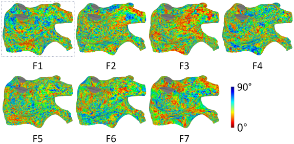
Figure 3: Local differences between endocardial and epicardial fiber orientations ($\Delta\theta$ maps) in the ground-truth F1 (box on the top left panel) and chimeric models of the left atrium (F2 to F7). Red and blue colors represent small and large $\Delta\theta$, respectively. Random local color variations indicate lack of large regions with the same $\Delta\theta$ value.

Table II shows the relative area occupied by smaller $\Delta\theta$ regions ($\Delta\theta\leq 45^{\circ}$) in different atria. Areas with smaller $\Delta\theta$ manifest higher effective anisotropy, which contributes to increased sensitivity of activation patterns to fiber organisation.

Table II: $\Delta\theta$ area analysis

F1	F2	F3	F4	F5	F6	F7
57%	56%	65%	55%	57%	53%	64%

Percentage of the atrium area occupied by regions with $\Delta\theta\leq 45^{\circ}$ in different models.

III-C Fibers do not significantly affect activation pattern

III-C1 Local activation time

To test the effects of fiber organization on activation patterns, we generated 42 simulations: six pacing sites each with seven different fiber patterns. The six pacing sites, shown in Fig. 1(e), are P1: Right Inferior Pulmonary Vein (RIPV), P2: Left Inferior Pulmonary Vein (LIPV), P3: Right Superior Pulmonary Vein (RSPV), P4: Left Superior Pulmonary Vein (LSPV), P5: Mitral Valve (MV), and P6: Bachmann’s Bundle (BB).

The resulting LAT maps are shown in Fig. 4. All maps are on $M_{endo1}$. The first column shows the simulation results in the ground-truth model built upon the intrinsic left atrium geometry and the fiber $F_{endo1}$ and $F_{epi1}$. Columns 2-7 are LAT maps obtained in models in which the intrinsic fiber was substituted with other fibers. The LAT maps of each row are similar, indicating that differences in fiber organization do not significantly affect the activation pattern.

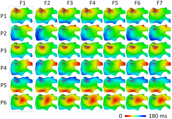
Figure 4: LAT maps produced by pacing from six different locations in the ground-truth (column F1) and chimeric models (columns F2 to F7). Color scales are normalized to each individual map. The maps in each row are similar to each other, demonstrating that despite significant differences in fiber patterns the activation pattern is not significantly affected.

To compare quantitatively the activation maps generated using the chimeric models with the ground-truth we calculated LAT errors (see Table III). The average LAT error is 7.8 ms, which is relatively small compared to the time it takes for the activation to travel through the entire left atrium (4.3% of 180 ms). The LAT correlation is also quite high ranging between 0.94 and 0.99 for different pacing sites and across all models. Also, we noticed that average LAT error (Table III bottom row) correlates with the relative size of the region with small $\Delta\theta$ (Table II).

Table III: absolute LAT error (ms)

	F2	F3	F4	F5	F6	F7	Avg
P1	4.6	6.1	5.5	4.2	5.7	5.0	5.2
P2	6.0	9.7	4.0	4.9	5.7	6.3	6.1
P3	9.0	11.5	7.1	8.8	10.4	12.5	9.9
P4	12.1	9.3	7.0	9.7	6.9	9.5	9.1
P5	13.8	7.5	13.6	3.8	6.7	7.8	8.9
P6	7.2	8.1	7.5	6.5	6.6	8.4	7.4
Avg	8.8	8.7	7.5	6.3	7.0	8.3	7.8

The last row shows the average LAT errors across all pacing sites in different fiber models, the last column shows the average error for a given pacing site across different models. The overall average is 7.8 ms or 4.3% of the LAT range (which is 180 ms).

III-C2 Latest activation location

Fig. 5 shows the latest activation locations in the left atrium. Blue regions indicate where LAT values are within 5 ms of the maximum LAT; The first column shows the results obtained in the ground-truth model with the intrinsic fiber pattern. Other columns are results obtained with different fiber organizations. Notably, in most of cases, the regions of late activation have similar locations, indicating that different fiber organizations do not alter the start-to-end activation wave patterns significantly. For example, rows P3 and P6 have consistent latest activation locations regardless of fiber organization; rows P2 and P4 show some instances with dilated regions, and row P1 has some different locations, but the clusters are still on the opposite side of the pacing site, which means the general activation pattern remains the same.

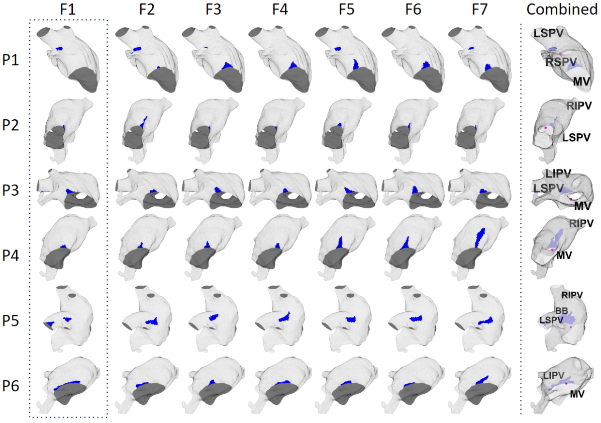
Figure 5: The regions of the latest activation derived from the activation maps shown in Fig. 4. The view angles are adjusted for each of pacing sites for better visualization. The first column (boxed) shows the results in the ground-truth model. Blue regions show the sites with the LAT values within 5 ms from the maximum. The average maximum LAT of the 42 scenarios is 180 ms. The last column shows the superposition of the latest activation regions for all fiber organizations. The magenta dots show the pacing sites on the back side of the atrium. For a given pacing site, the position of the blue regions are reasonably well preserved across different fiber organizations.

Table IV: latest activation location difference (mm)

	F2	F3	F4	F5	F6	F7	Avg
P1	3.37	34.63	38.75	16.80	38.30	24.17	26.00
P2	6.95	1.86	1.73	8.02	1.38	3.17	3.85
P3	17.28	14.10	15.83	10.72	10.60	12.62	13.52
P4	2.95	3.16	4.24	6.13	6.32	17.12	6.65
P5	26.09	18.61	26.81	26.09	23.61	27.40	24.77
P6	9.72	4.68	5.23	2.49	8.33	5.78	6.04
Avg	11.06	12.84	15.43	11.71	14.76	15.04	13.47

Latest activation location difference is the distance between the center of the blue area for F2-F7 and F1 (the truth). The mean is 13.47 mm and the median is 9.43 mm, which are relatively small compared to the left atrium size, indicating that the latest activation locations for different fiber organizations are similar. Note that the values in rows P5 and P6 are very different, which demonstrates that the latest activation location differences depend on pacing location.

The quantitative analysis is summarized in Table IV. For each simulation illustrated in Fig. 5 columns F2-F7, we compute the distance of the center of the blue area to the truth. For most scenarios, the distances are small (median: 9.43 mm; average: 13.47 mm) compared to the size of the left atrium mesh $M_{endo1}$ (84 mm $\times$ 97 mm $\times$ 88 mm). Notably, the average across different pacing sites does not change significantly from model to model (see the last row in Table IV). Yet, for some pacing sites, they are consistently better than for other pacing sites, for example, compare rows P5 and P6.

III-D Fibers have local effects on activation propagation

Although differences in fiber organization have little effect on the large scale, they can be observed locally. Fig. 6 shows activation maps generated using models F2 and F3 paced at P2. The activation propagates in the direction of the red-dashed arrow. In the F2 row, the activation propagation slows down in the orange circled area (it has a smaller red region) because the fiber direction is perpendicular to the activation direction. In the F3 row, because fiber direction is along the activation direction, it accelerates propagation and results in a larger red area. Such acceleration and slow-down effects occur throughout the left atrium. The cyan-circled area is another example: propagation is slower in the F2 row than F3 row, resulted in more blue area.

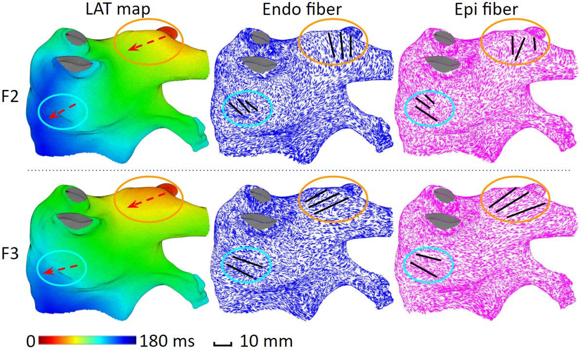
Figure 6: Local effect of fiber organization. Upper and lower panels show LAT maps (left) and fiber organization (center and right) in models F2 and F3, respectively. Red arrows: propagation direction. Black lines: prevailing fiber direction in the areas of interest (orange and cyan ovals). The LAT gradient inside the orange oval is conspicuously greater in F2 than in F3 (red-green vs red-yellow). This is because the endocardial and epicardial fibers in F2 are perpendicular to the activation direction, resulting in slower propagation. This is not the case for F3 where propagation is parallel to fibers. Such local effects exist throughout the entire atrium, but they do not alter the overall activation pattern much.

III-E Fiber effects with different anisotropy ratios

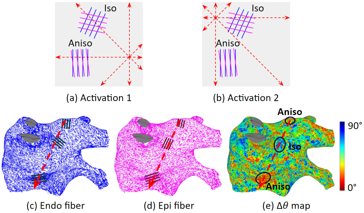
Figure 7: The cancellation effect explained via the fibers: there is no macro level consistent fiber organization, therefore local fiber effects cancel each other. (a, b) show fiber’s local effect. Blue lines represent endocardium fiber, magenta lines represent epicardium fiber. Aniso region has a small $\Delta\theta$ (about 0°), and Iso region has a large $\Delta\theta$ (about 90°). Red arrows are activation wave traveling directions. For activation scenario (a), The Aniso region has a slow down effect on the activation; However, for activation scenario (b), The Aniso region has a speed up effect on the activation. And for both (a) and (b), the propagation speed in the Iso region are similar. (c, d, e) show that the local effects cancel each other at the macro level. (c) is endocardium fiber, (d) is epicardium fiber, and (e) is $\Delta\theta$ map. Along the activation path marked by the red dashed arrow, the propagation speed increases in the top Aniso region, then it goes trough an Iso region that does not change the speed much, finally it enters the bottom Aniso region and the speed decreases. In summary, activation speed first increases then decreases, therefore the effects cancel each other.

Table V: Different anisotropy ratios

$r$	0.1	0.2	0.5
LAT Error (ms)	10.6 or 5.5%	7.8 or 4.3%	3.15 or 2.0%

The percentage is with respect to the time it takes the activation to travel through the left atrium. For r = 0.1, 0.2, 0.5, that time is 192, 180, 155 ms respectively.

The majority of simulations of atrial propagation use values of $r$ between 0.1 and 0.2. Some publications use $r=0.11$ [47, 48], while some others use $r=0.2$ [49]. To investigate the robustness of our conclusions, we performed the same experiment as described in Section III-C with $r=0.1$ and $r=0.5$, and the results are summarized in Table V. The small errors suggest that the anisotropy ratio is not the main factor responsible for the low sensitivity of the large scale activation patterns to specific fiber organization.

III-F Uncouple the two fiber layers

The reason for fiber organization having little effect on the activation patterns at the large scale could be partly due to significant differences in fiber orientation on the epicardial and endocardial layers (see Fig. 3) which cause reduction in apparent anisotropy. But the left atrial wall was not always two layers in all parts [5, 50]. To evaluate the contribution of this effect on the large scale activation we generated seven models in which epicardial layers were assigned the endocardial fiber orientations, thus producing identical fiber orientation in both layers, which is equivalent to completely uncouple the endocardial layer from the epicardium.

We hypothesized that this modification should amplify the apparent anisotropy, and consequently the differences between activation patterns in different models. Using these modified models, we performed the same experiment as described in Section III-C and compared the results. It might be expected, the errors in LAT in the models with identical epicardial and endocardial fiber orientations was greater than in the original models, however, the difference was not very large (9.1 ms vs 7.8 ms).

This suggests that the difference in the endocardium and epicardium fiber orientations is not the main factor responsible for low sensitivity of the large scale activation patterns to specific fiber organization.

IV Discussion

IV-A Contemporary heart modeling with fibers

Electrophysiological heart modeling is becoming increasingly realistic with an aim to guide atrial fibrillation ablation procedures. One important element of a heart model is the fiber organization. However, accurate and high-resolution fiber data is not available for clinical use. The major difficulty of obtaining such in-vivo fiber organization is the time it takes to scan the fibers. The current DT-MRI technology can scan high-resolution fibers in about 50 hours [38], which is clinically impractical.

One way to quickly obtain fiber organization is to mathematically calculate synthetic fibers based on atrial geometry [8, 51, 52, 53, 54]. However, these fibers are artificial and do not represent the truth. Another option is to register foreign fibers. It has been found that one certain patient’s atrial fiber organization can be generalized to many different patients [39].

In this paper, we tried an alternative way, we ask the question: how big an effect does fiber organization have on activation patterns? If the effects are small, then we could create a clinically practical heart model that does not involve fiber data.

IV-B Cancellation effect

Our data suggest that the effects of fiber organizations are cancelled because fiber organizations vary across the left atrium. This cancellation effect can be explained at two levels.

At the micro level, depending on the location of the activation origin, wave propagation can be shaped by the local fiber organization. As shown in Fig. 7(a, b), they represent the same tissue region but has different activations. Aniso region has small $\Delta\theta$ (about 0°), it is highly anisotropic, and have the strongest local effect on activation propagation; Iso region has large $\Delta\theta$ (about 90°), it is highly isotropic, and have the least effect on activation propagation. For Iso region, activation waves will travel through them in a similar manner regardless of the direction of travel. For Aniso region, depends on the direction of the activation wave, its travelling speed can be decreased (as shown in (a)) or increased (as shown in (b)).

At the macro level, the local effects from the micro level will be cancelled by each other. As shown in Fig. 7(c, d, e), along a global path, the activation wave can travel through areas that increase and areas that decrease propagation speed, resulting in an overall zero effect.

Quantitatively, the propagation speed along a path is shown in Fig. 8. The path is the geodesic line (minimum distance path) from the activation origin (point A) to the latest activation location (point B) as shown in (a), and it can be found via Dijkstra’s algorithm. The path has a length of about 120 mm. The propagation speed of a point along the path is calculated as distance divided by time, where distance is the geodesic length from that point to point A, and the time is the LAT values difference between that point and point A. We can see that the propagation speeds vary around its average value along the path as shown in (b), and the average propagation speeds are similar regardless of fiber organizations as shown in (c). Such phenomenon happened for all 42 scenarios. Because of this phenomenon, the fiber organization’s local effect does not accumulate along the path, resulting in a small macro effect.

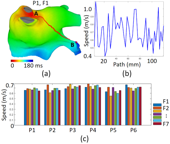
Figure 8: An example of propagation speed along a path. (a) The path (red line) is the geodesic line from the earliest (point A) to the latest activation location (point B). (b) The path’s value is the geodesic length from the point along the path to point A. We can see that the propagation speed increases and decreases along the path. (c) The bar plots are the average propagation speed. We can see that for all the six different pacing scenarios, the average propagation speed values are similar regardless of which fiber organization was implemented. (Note that propagation speed is not necessarily equal to CV, because CV is in the LAT gradient direction while the path is not necessarily aligned with that. We did not compute CV along the path because it is not easy to get accurate results [55].)

IV-C Potential applications: fiber-independent model

In our previous research [56], we showed that we can construct a model of the left atrium to reproduce clinical electroanatomical mapping data [57] without incorporating fiber organization. We validated our fiber-independent model with data from 15 patients and the performance was good: the average absolute LAT error was 5.47 ms for sinus rhythm and 10.97 ms for flutter and tachycardia, and the average correlation was 0.95 for sinus rhythm and 0.81 for flutter and tachycardia. There are also other studies support the use of heart model without fibers [58, 59, 60].

In this work, because we found that fibers did not significantly affect activation patterns, we expect that the fiber-independent model can be useful for predicting fibrillation source locations. Because the fiber-independent model only requires heart geometry and electrograms, it could be integrated into contemporary electroanatomical mapping systems to provide real-time atrial fibrillation ablation guidance.

V Limitations

We found that fiber organization does not significantly affect activation patterns. However, there are important limitations to the scenarios we considered that informed this finding.

1) We focused only on sustained sources, such as focal atrial tachycardia, which may occur following atrial fibrillation ablation. It is possible that non-stationary sources such as drifting rotors could be affected by fibers.

2) We did not consider scars, which could play an important role in atrial fibrillation dynamics [61].

3) The Mitchell-Schaeffer model we used is not a detailed ionic model, and it may not be a good choice to model complex rhythms such as atrial fibrillation. Still such a two-component model is good for modeling periodic propagation. We utilized the computationally more efficient mono-domain model. It is well established that more detailed bi-domain models are required for accurate simulation of electrical activity in the immediate vicinity of the stimulating electrodes and for modelling electrical defibrillation [62]. With regard to accuracy, the bi-domain models have practically no advantages over mono-domain models for simulations of propagation patterns of external stimulus [63].

4) We simplify fiber organization into only two layers. The real left atrium has many more layers, and the number of layers also varies in different regions, as does the atrial thickness. If more layers were incorporated, we would need to study if the effects of fibers would become stronger as well as whether the fiber direction changes abruptly or gradually through the thickness.

5) We examined fiber organizations of the left atrium, because the most common atrial fibrillation sources are in the left atrium; therefore, it has more available clinical electroanatomical mapping data than the right atrium. We have not examined whether our findings would hold in the right atrium.

VI Conclusion

In this paper, we found that 1) Fiber organization varies significantly across different left atria and within a left atrium. 2) Fibers have local effects on activation propagation but such local effects cancel each other at the macro level. And 3) fibers do not significantly affect activation pattern.

In summary, for left atrial focal arrhythmia, we found that the global activation patterns do not seem to be significantly affected by fiber organization. Therefore, fiber organization may not be essential for accurate heart modeling of arrhythmias in the left atrium, and thus more practical heart models for some clinical applications could be fiber-independent models. It has been shown that there is an asynchrony and dissociation between activation on the epicardium and endocardium during atrial arrhythmias [64, 65, 66]; these and our results further suggest that it may be more important to consider the role of the complex trabecular network [66, 67, 10] during arrhythmias.

Appendix A Fiber registration

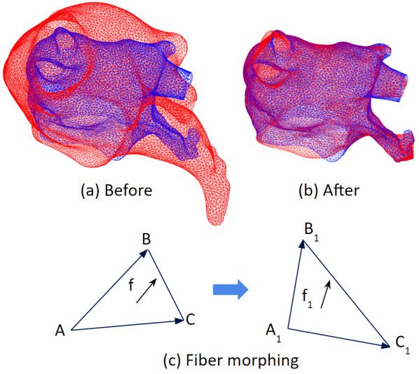
Figure 9: Fiber registration. (a) and (b) are the before and after mesh morphing. (c) shows how to transform fiber from the original mesh (red mesh in (a)) to the morphed mesh (red mesh in (b)): Given xyz coordinates of $A$, $B$, $C$, $A_{1}$, $B_{1}$, $C_{1}$, and the fiber (3D vector $f$), calculate $f_{1}$. We have $f=a\textbf{AB}+b\textbf{AC}$, by solving for $a$ and $b$, we can obtain $f_{1}=a\textbf{A}_{1}\textbf{B}_{1}+b\textbf{A}_{1}\textbf{C}_{1}$, then make $f_{1}$ unit length, it will be the morphed fiber. (Note that $f=a\textbf{AB}+b\textbf{AC}$ will give 3 equations, since AB, AC and $f$ are co-plane, any 2 of the 3 equations will give the same $a$ and $b$.)

The seven endocardium and seven epicardium fibers are registered onto the left atrium 1’s endocardium mesh. Name left atrium 1’s endocardium the target mesh, other endocardium or epicardium mesh a moving mesh. First, rotate the moving mesh to roughly align with the target mesh. Next, apply a rigid ICP algorithm to optimize the alignment. Lastly, apply a non-rigid ICP algorithm to morph the moving mesh into the shape of the target mesh [68]. Fig. 9 shows an example of the mesh morphing. The blue mesh is the target mesh, the red mesh (can be endocardium or epicardium) is the moving mesh. (a) shows the original meshes. (b) shows the red mesh is morphed into the shape of the blue mesh. We can see that the morphed mesh matches the target well, on average, the distance between the nearest vertex pairs between the morphed mesh and the target mesh is: 1.4 +/- 0.5 mm. Then we need to morph the fiber data. (c) shows the process: it is a reference frame transformation. The final step is to register the morphed fiber to the target mesh, this can be done by copying the fibers that are nearest to the target mesh’s triangles.

Appendix B Compare different fiber organizations

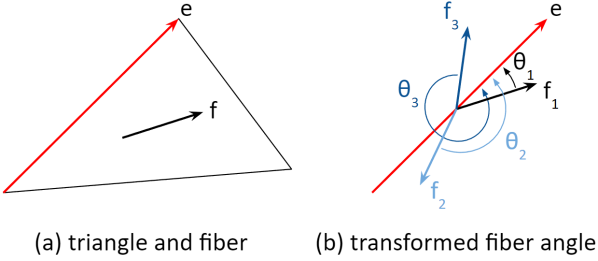
Figure 10: Transform fiber data. (a) Fiber $f$ resides in a triangle of the mesh. The reference vector $e$ created from a fixed edge, all the seven different fibers will reference this vector $e$. (b) The 3D fiber vector is transformed into a 1D value. Examples of fibers ($f_{1}$, $f_{2}$, and $f_{3}$) and their transformed values ($\theta_{1}$, $\theta_{2}$, and $\theta_{3}$).

There are seven different fiber organizations registered onto the left atrium 1’s endocardium mesh. Fibers are 3D vectors as shown in Fig. 10(a), it is not convenient to directly compute correlations among 3D vectors. Therefore, we make a reference frame transformation so that the 3D fibers ($f_{1}$, $f_{2}$, and $f_{3}$) are represented as 1D values ($\theta_{1}$, $\theta_{2}$, and $\theta_{3}$) as shown in (b). The reference frame is a vector created by a fixed edge of each triangle (vector $e$ in (a)), and the transformation is to compute the angle between the fiber and that fixed edge ($\theta$ in (b)) follow the right hand rule of the triangle face normal vector. (Note that it is a property of a triangular mesh, that the sequence of the 3 vertices of a triangle are in such a way that we can utilize the right-hand-rule to find out the triangular face normal vector that points outwards of the mesh.) After this transformation, we can easily compute the correlations between different fiber organizations.

Appendix C Spatial and temporal resolutions

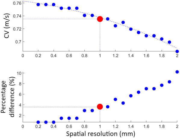
Figure 11: Top: Conduction velocity (CV) values (the dots) of implementing different resolutions. The dashed blue line is a quadratic fit of the dots. Bottom: CV percentage differences compare to the asymptotic value, which is the value of the dashed blue line at 0 mm spatial resolution. For spatial resolution of 1 mm and temporal resolution of 0.01 ms (the big red dot), the CV percentage difference is 3.6%, much smaller than the adequate 10%.

We ran simulations on a slab of 100 mm $\times$ 4 mm $\times$ 4 mm. (The long length of the slab is to help increase CV computational accuracy.) The heart model parameters are chosen such that the CV values are close to the physical values [69]. Assume isotropic conduction, or no fiber organization. Spatial resolutions are set to 0.2, 0.3, …, 2.0 mm. Temporal resolution $dt$ is set to 0.01 ms. Results are summarized in Fig. 11. In this paper, spatial resolution is 1 mm and temporal resolution is 0.01 ms. Using such resolutions, the accuracy of CV is adequate with a deviation from the asymptotic value of 3.6%, which is much smaller than the usual required 10%.

References

- [1] T. O’Hara et al., “Simulation of the undiseased human cardiac ventricular action potential: model formulation and experimental validation,” PLoS computational biology, vol. 7, no. 5, p. e1002061, 2011.
- [2] D. Greene et al., “Voltage-mediated mechanism for calcium wave synchronization and arrhythmogenesis in atrial tissue,” Biophysical Journal, vol. 121, no. 3, pp. 383–395, 2022.
- [3] F. H. Fenton and E. M. Cherry, “Models of cardiac cell,” Scholarpedia, vol. 3, no. 8, p. 1868, 2008.
- [4] S. Ho et al., “Anatomy of the left atrium: implications for radiofrequency ablation of atrial fibrillation,” Journal of cardiovascular electrophysiology, vol. 10, p. 1525—1533, November 1999.
- [5] Y. Ho and D. Sánchez-Quintana, “The importance of atrial structure and fibers,” Clin Anat, vol. 22, no. 1, pp. 52–63, 2009.
- [6] P. A. Iaizzo, “The visible heart® project and free-access website ‘atlas of human cardiac anatomy’,” EP Europace, vol. 18, no. suppl_4, pp. iv163–iv172, 2016.
- [7] S. Ho et al., “Architecture of the pulmonary veins: relevance to radiofrequency ablation,” Heart, vol. 86, no. 3, pp. 265–270, 2001.
- [8] T. E. Fastl et al., “Personalized computational modeling of left atrial geometry and transmural myofiber architecture,” Medical Image Analysis, vol. 47, pp. 180–190, 2018.
- [9] A. Lopez-Perez et al., “Three-dimensional cardiac computational modelling: methods, features and applications,” BioMedical Engineering OnLine, vol. 14, p. 35, 2015.
- [10] J. P. Berman et al., “Interactive 3d human heart simulations on segmented human mri hearts,” in 2021 Computing in Cardiology (CinC), vol. 48, pp. 1–4, IEEE, 2021.
- [11] A. Kaboudian et al., “Real-time interactive simulations of large-scale systems on personal computers and cell phones: Toward patient-specific heart modeling and other applications,” Science advances, vol. 5, no. 3, p. eaav6019, 2019.
- [12] J. N. Weiss et al., “Electrical restitution and cardiac fibrillation,” Journal of cardiovascular electrophysiology, vol. 13, no. 3, pp. 292–295, 2002.
- [13] M. A. Watanabe et al., “Mechanisms for discordant alternans,” Journal of cardiovascular electrophysiology, vol. 12, no. 2, pp. 196–206, 2001.
- [14] F. Fenton and A. Karma, “Fiber-rotation-induced vortex turbulence in thick myocardium,” Physical review letters, vol. 81, no. 2, p. 481, 1998.
- [15] W. Groenendaal et al., “Voltage and calcium dynamics both underlie cellular alternans in cardiac myocytes,” Biophysical journal, vol. 106, no. 10, pp. 2222–2232, 2014.
- [16] I. Uzelac et al., “Simultaneous quantification of spatially discordant alternans in voltage and intracellular calcium in langendorff-perfused rabbit hearts and inconsistencies with models of cardiac action potentials and ca transients,” Frontiers in physiology, vol. 8, p. 819, 2017.
- [17] H. J. Arevalo et al., “Arrhythmia risk stratification of patients after myocardial infarction using personalized heart models,” Nature communications, vol. 7, no. 1, pp. 1–8, 2016.
- [18] E. Kayvanpour et al., “Towards personalized cardiology: multi-scale modeling of the failing heart,” PLoS One, vol. 10, no. 7, p. e0134869, 2015.
- [19] S. Niederer et al., “Creation and application of virtual patient cohorts of heart models,” Philosophical Transactions of the Royal Society A, vol. 378, no. 2173, p. 20190558, 2020.
- [20] M. C. Sanguinetti and P. B. Bennett, “Antiarrhythmic drug target choices and screening,” Circulation Research, vol. 93, no. 6, pp. 491–499, 2003.
- [21] J. Bai et al., “In silico study of the effects of anti-arrhythmic drug treatment on sinoatrial node function for patients with atrial fibrillation,” Scientific reports, vol. 10, no. 1, pp. 1–14, 2020.
- [22] I. Uzelac et al., “Quantifying arrhythmic long qt effects of hydroxychloroquine and azithromycin with whole-heart optical mapping and simulations,” Heart Rhythm O2, vol. 2, no. 4, pp. 394–404, 2021.
- [23] P. Mamoshina et al., “Toward a broader view of mechanisms of drug cardiotoxicity,” Cell Reports Medicine, vol. 2, no. 3, p. 100216, 2021.
- [24] D. Duncker and C. Veltmann, “Optimizing antitachycardia pacing,” Circulation: Arrhythmia and Electrophysiology, vol. 10, no. 9, p. e005696, 2017.
- [25] Y. C. Ji et al., “Synchronization as a mechanism for low-energy anti-fibrillation pacing,” Heart rhythm, vol. 14, no. 8, pp. 1254–1262, 2017.
- [26] N. DeTal et al., “Terminating spiral waves with a single designed stimulus: Teleportation as the mechanism for defibrillation,” Proceedings of the National Academy of Sciences, vol. 119, no. 24, p. e2117568119, 2022.
- [27] B. Lim et al., “In situ procedure for high-efficiency computational modeling of atrial fibrillation reflecting personal anatomy, fiber orientation, fibrosis, and electrophysiology,” Scientific Reports, vol. 10, p. 2417, 2020.
- [28] A. Prakosa et al., “Personalized virtual-heart technology for guiding the ablation of infarct-related ventricular tachycardia,” Nature biomedical engineering, vol. 2, no. 10, pp. 732–740, 2018.
- [29] P. Pathmanathan et al., “Comprehensive uncertainty quantification and sensitivity analysis for cardiac action potential models,” Frontiers in physiology, vol. 10, p. 721, 2019.
- [30] P. Pathmanathan et al., “Data-driven uncertainty quantification for cardiac electrophysiological models: Impact of physiological variability on action potential and spiral wave dynamics,” Frontiers in physiology, vol. 11, p. 585400, 2020.
- [31] R. Doste et al., “A rule-based method to model myocardial fiber orientation in cardiac biventricular geometries with outflow tracts,” International journal for numerical methods in biomedical engineering, vol. 35, no. 4, p. e3185, 2019.
- [32] J. D. Bayer et al., “A novel rule-based algorithm for assigning myocardial fiber orientation to computational heart models,” Annals of biomedical engineering, vol. 40, no. 10, pp. 2243–2254, 2012.
- [33] M. Valderrábano, “Influence of anisotropic conduction properties in the propagation of the cardiac action potential,” Progress in Biophysics and Molecular Biology, vol. 94, no. 1, pp. 144–168, 2007. Gap junction channels: from protein genes to diseases.
- [34] P. C. Franzone et al., “Spread of excitation in a myocardial volume: Simulation studies in a model of anisotropic ventricular muscle activated by point stimulation,” Journal of cardiovascular electrophysiology, vol. 4, no. 2, pp. 144–160, 1993.
- [35] F. Fenton and A. Karma, “Vortex dynamics in three-dimensional continuous myocardium with fiber rotation: Filament instability and fibrillation,” Chaos: An Interdisciplinary Journal of Nonlinear Science, vol. 8, no. 1, pp. 20–47, 1998.
- [36] D. Bhakta and J. Miller, “Principles of electroanatomic mapping,” Indian Pacing Electrophysiol J., vol. 1, no. 8, pp. 32–50, 2008.
- [37] J. Zhao et al., “An image-based model of atrial muscular architecture,” Circulation: Arrhythmia and Electrophysiology, vol. 5, no. 2, pp. 361–370, 2012.
- [38] F. Pashakhanloo et al., “Myofiber architecture of the human atria as revealed by submillimeter diffusion tensor imaging,” Circulation: Arrhythmia and Electrophysiology, vol. 9, no. 4, p. e004133, 2016.
- [39] C. H. Roney et al., “Constructing a human atrial fibre atlas,” Annals of Biomedical Engineering, vol. 49, p. 233–250, 2021.
- [40] J. Whitaker et al., “The role of myocardial wall thickness in atrial arrhythmogenesis,” EP Europace, vol. 18, pp. 1758–1772, 05 2016.
- [41] J. Y. Sun et al., “Left atrium wall-mapping application for wall thickness visualisation,” Sci Rep, vol. 8, p. 4169, 2018.
- [42] C. C. Mitchell and D. G. Schaeffer, “A two-current model for the dynamics of cardiac membrane,” Bulletin of Mathematical Biology, vol. 65, p. 767–793, 2003.
- [43] I. Elaff, “Modeling of realistic heart electrical excitation based on dti scans and modified reaction diffusion equation,” Turkish Journal of Electrical Engineering & Computer Sciences, vol. 26, no. 3, pp. 1153–1163, 2018.
- [44] R. McFarlane, “High-performance computing for computational biology of the heart,” Doctor in Philosophy thesis of the University of Liverpool, School of Electrical Engineering, Electronics and Computer Science, p. 132, 2010.
- [45] R. Cabrera-Lozoya et al., “Image-based biophysical simulation of intracardiac abnormal ventricular electrograms,” IEEE Transactions on Biomedical Engineering, vol. 64, no. 7, pp. 1446–1454, 2017.
- [46] C. H. Roney et al., “A technique for measuring anisotropy in atrial conduction to estimate conduction velocity and atrial fibre direction,” Computers in Biology and Medicine, vol. 104, pp. 278–290, 2019.
- [47] T. D. Coster et al., “Myocyte remodeling due to fibro-fatty infiltrations influences arrhythmogenicity,” Front. Physiol., vol. 9, p. 1381, 2018.
- [48] O. V. Aslanidi et al., “3d virtual human atria: A computational platform for studying clinical atrial fibrillation,” Prog Biophys Mol Biol, vol. 107(1), pp. 156–68, 2011.
- [49] P. M. Boyle et al., “Computationally guided personalized targeted ablation of persistent atrial fibrillation,” Nature Biomedical Engineering, vol. 3, p. 870–879, 2019.
- [50] Y. Ho et al., “Left atrial anatomy revisited,” Circulation: Arrhythmia and Electrophysiology, vol. 5, no. 1, pp. 220–228, 2012.
- [51] M. W. Krueger et al., “Modeling atrial fiber orientation in patient-specific geometries: A semi-automatic rule-based approach,” in Springer Berlin Heidelberg, pp. 223–232, 2011.
- [52] S. Labarthe et al., “A semi-automatic method to construct atrial fibre structures: A tool for atrial simulations,” in 2012 Computing in Cardiology, pp. 881–884, 2012.
- [53] A. Wachter et al., “Mesh structure-independent modeling of patient-specific atrial fiber orientation,” Current Directions in Biomedical Engineering, vol. 1, no. 1, pp. 409–412, 2015.
- [54] A. Saliani et al., “Simulation of diffuse and stringy fibrosis in a bilayer interconnected cable model of the left atrium,” EP Europace, vol. 23, no. Supplement-1, pp. i169–i177, 2021.
- [55] C. D. Cantwell et al., “Techniques for automated local activation time annotation and conduction velocity estimation in cardiac mapping,” Computers in Biology and Medicine, vol. 65, pp. 229 – 242, 2015.
- [56] J. He et al., “Patient-specific heart model towards atrial fibrillation,” in Proceedings of the ACM/IEEE 12th International Conference on Cyber-Physical Systems, ICCPS ’21, (New York, NY, USA), p. 33–43, Association for Computing Machinery, 2021.
- [57] J. He et al., “Electroanatomic mapping to determine scar regions in patients with atrial fibrillation,” in 2019 41st Annual International Conference of the IEEE Engineering in Medicine and Biology Society (EMBC), pp. 5941–5944, 2019.
- [58] N. Virag et al., “Study of atrial arrhythmias in a computer model based on magnetic resonance images of human atria,” Chaos, vol. 12, no. 3, pp. 754–763, 2002.
- [59] R. P et al., “A biophysical model of atrial fibrillation ablation: what can a surgeon learn from a computer model?,” Europace, vol. 9, no. 6, pp. vi71–6, 2007.
- [60] G. RA et al., “Incomplete reentry and epicardial breakthrough patterns during atrial fibrillation in the sheep heart,” Circulation, vol. 94, no. 10, pp. 2649–61, 1996.
- [61] M. Gonzales et al., “Structural contributions to fibrillatory rotors in a patient-derived computational model of the atria,” Europace, pp. iv3–iv10, 2014.
- [62] B. J. Roth, “Bidomain modeling of electrical and mechanical properties of cardiac tissue,” Biophysics Reviews, vol. 2, no. 4, p. 041301, 2021.
- [63] M. Potse et al., “A comparison of monodomain and bidomain reaction-diffusion models for action potential propagation in the human heart,” IEEE Transactions on Biomedical Engineering, vol. 53, no. 12, pp. 2425–2435, 2006.
- [64] N. de Groot et al., “Direct proof of endo-epicardial asynchrony of the atrial wall during atrial fibrillation in humans,” Circulation: Arrhythmia and Electrophysiology, vol. 9, no. 5, p. e003648, 2016.
- [65] J. Eckstein et al., “Transmural conduction is the predominant mechanism of breakthrough during atrial fibrillation: evidence from simultaneous endo-epicardial high-density activation mapping,” Circulation: Arrhythmia and Electrophysiology, vol. 6, no. 2, pp. 334–341, 2013.
- [66] S. Verheule et al., “Role of endo-epicardial dissociation of electrical activity and transmural conduction in the development of persistent atrial fibrillation,” Progress in biophysics and molecular biology, vol. 115, no. 2-3, pp. 173–185, 2014.
- [67] T.-J. Wu et al., “Role of pectinate muscle bundles in the generation and maintenance of intra-atrial reentry: potential implications for the mechanism of conversion between atrial fibrillation and atrial flutter,” Circulation research, vol. 83, no. 4, pp. 448–462, 1998.
- [68] B. Amberg et al., “Optimal step nonrigid icp algorithms for surface registration,” in 2007 IEEE Conference on Computer Vision and Pattern Recognition, pp. 1–8, 2007.
- [69] D. M. Harrild and C. S. Henriquez, “A computer model of normal conduction in the human atria,” Circulation Research, vol. 87, no. 7, pp. e25–e36, 2000.