QuDPy: A Python-based Tool For Computing Ultrafast Non-linear Optical Responses

Abstract

Nonlinear Optical Spectroscopy is a well-developed field with theoretical and experimental advances that have aided multiple fields including chemistry, biology and physics. However, accurate quantum dynamical simulations based on model Hamiltonians are needed to interpret the corresponding multi-dimensional spectral signals properly. In this article, we present the initial release of our code, QuDPy (quantum dynamics in python) which addresses the need for a robust numerical platform for performing quantum dynamics simulations based on model systems, including open quantum systems. An important feature of our approach is that one can specify various high-order optical response pathways in the form of double-sided Feynman diagrams via a straightforward input syntax that specifies the time-ordering of ket-sided or bra-sided optical interactions acting upon the time-evolving density matrix of the system. We use the quantum dynamics capabilities of QuTip for simulating the spectral response of complex systems to compute essentially any $n^{th}$-order optical response of the model system. We provide a series of example calculations to illustrate the utility of our approach.

PROGRAM SUMMARY

Program Title: QuDPy
CPC Library link to program files: (to be added by Technical Editor)
Developer’s repository link: https://github.com/sa-shah/QuDPy
Code Ocean capsule: (to be added by Technical Editor)
Licensing provisions: MIT License (MIT License Copyright (c) 2022 Syed A shah)
Programming language: Python (v3.7)
Computer: Any architecture with Python (v3.7)
Operating system: Linux, MacOS
Supplementary material: Available as Google Colab Files.
Example 1: https://tinyurl.com/y3j5jmmr
Example 2: https://tinyurl.com/37vwntn5

Required (External) packages:

• QuTip (v.4.7) and dependencies i.e. Numpy, Matplotlib ( https://qutip.org/)

• UFSS Automatic Diagram Generator (https://github.com/peterarose/ufss)

Has the code been vectorised or parallelized?: Yes, parallelized within QuTip (v4.7) using MPI.
Nature of problem(approx. 50-250 words):
Accurate quantum simulations of complex systems are required in order to understand and interpret multi-dimensional ultrafast spectroscopic signals. This code provides an open-source/multi-platform method that facilitates the generation of higher-order non-linear optical responses for an arbitrary molecular or material system given a model input Hamiltonian and bath model.
Solution method(approx. 50-250 words):
We use the double-sided Feynman diagram method [1, 2] to generate (symbolically) a set of response functions corresponding to the $n^{th}$ order non-linear response of the system to a series of laser pulses using the UFSS package[3] We then perform a series of accurate quantum dynamics calculations using the QuTip package[4] to generate the numerical response and spectra which correspond to specific experimental conditions.

Additional comments including restrictions and unusual features (approx. 50-250 words):
None.

1 Introduction

Nonlinear, ultrafast spectroscopy has emerged as powerful experimental tool for probing coherent, light-induced processes in the condensed phase. [1, 2, 3, 4, 5, 6] In this technique, one prepares a sequence of ultra-narrow (in time) optical pulses, with specific phase matching conditions, that induce a macroscopic polarization response. This polarization is directly linked to the time-evolution of the sample under investigation. By varying the time intervals between phase-matched pulses one can develop a multi-dimensional map correlating the absorption at one time with emission at some later time. By comparing the experimental signals against robust theoretical models, one can gain tremendous insight into the inner quantum dynamics of a complex system.

The field itself is mature and two textbook-level works are considered as the general introduction in this field. [7, 8] However, setting up and performing accurate quantum simulations of complex systems, along with their interaction with the thermal environment has long been the purview of theoretical groups. As a result, the community currently lacks a universal and portable code for performing such simulations. We present our implementation of a general platform for computing the ultrafast optical response for a generalized system that can be described in terms of a model Hamiltonian in contact with a dissipative environment. Our platform can simulate a wide range of molecular and condensed matter systems with finite-dimensional model Hamiltonians. It offers simulation capabilities across a broad spectral range (from NMR to UV-Vis), encompassing various transitions such as electronic, vibrational, rotational, and more. Our code, written in Python 3, leverages the open-source QuTip quantum simulation package.[9] It provides the user with a straightforward way to automatically generate and compute non-linear responses, as specified by a double-sided Feynman diagram given as input. The double-sided diagrams are created using the Automatic Feynman Diagram Generator within the UFSS package, tailored to the desired phase-matching or phase-cycling condition.[10, 11]

Our platform currently simulates non-linear responses in the impulsive regime, applicable to a significant number of ultra-fast optics experiments. However, this simulation does not include electric field polarization. Future releases will enhance the capabilities by covering both the non-impulsive regime and resolving electric field polarization.

It is worth pointing out the other notable efforts on computational fronts in ultrafast optical spectroscopy. The Spectron/iSpectron by Mukamel et. al. provides the spectral calculations via two methods. Firstly, though the average amplitudes of Liouville pathways and cumulant expansion of Gaussian fluctuations in reference eigen-energies; and secondly with the use of the molecular configuration specific Green’s function expressions.[12] On the other hand, the Ultrafast Spectroscopy Suit (UFSS) by Ross and Kirch obtains the nonlinear spectroscopic signatures (for both closed and open quantum systems with finite-dimensional Hilbertspace) via perturbative expansion of wavefunction, and conversion of light-matter interaction with subsequent evolution into a convolution problem with appropriately designed operators. Their method takes into account the temporal profiles of the laser pulses. This results in reduced computational cost for simulation, especially in the case of temporal overlap between different laser pulses. Additionally, the suit provides automatic generation of double-sided Feynman diagrams that has been utilized in this work. [10, 11] Briefly, our approach differentiates itself from these routines by computing the direct evolution of density matrix for the system with intermittent projection with light-matter interaction defining and guiding specific Liouville pathways.

We begin with a general overview of the theory of multi-dimensional spectroscopy, its implementation in our code, and describe its installation and required components. We then present a few model calculations showing how one can setup, compute, and interpret the results. Our intention is that the code provides a robust and adaptable platform for both theory and experimental groups working in this area. To maintain the brevity of the article, the complete code for these simulations is available in Examples 1 and 2 on the Google Colab platform and the input parameters for various functions and methods in the package are thoroughly explained in the Appendix.

2 Theoretical background and description of the algorithm

In any spectroscopic experiment, one ultimately is measuring a macroscopic polarization of the sample as induced by an incident applied electric field and one can express the polarization in terms of powers of the electric field $\vec{E}$

$$\vec{P}=\epsilon_{o}\left(\chi^{(1)}\cdot\vec{E}+\chi^{(2)}\cdot\vec{E}\cdot\vec{E}+\chi^{(3)}\cdot\vec{E}\cdot\vec{E}\cdot\vec{E}+\cdots\right)$$ (1)

where $\chi^{(n)}$ are susceptibilities. Since the electric field is a vector, the various susceptibilies are in fact tensors. In isotropic media with inversion symmetry, the polarization must change sign when the optical electric fields are reversed. Consequently, all the even-order terms vanish and the 3rd order term is the lowest-order non-linearity.

Under the dipole approximation in light-matter interaction, the observed polarizability is calculated by taking the expectation value of the quantum dipole operator:

$$P(t)=\text{Tr}(\mu\rho(t))=\langle\mu\rho(t)\rangle$$ (2)

where $\rho(t)$ is the quantum density matrix for the system which has evolved under the influence of the external optical fields. This, too, can be expanded in powers of the electric field as

$$P(t)=\sum_{n=1}^{\infty}P^{(n)}(t)$$ (3)

Each of the terms in this series can be computed within the context of time-dependent perturbation theory by assuming that the applied fields interacts with the system at times $\tau_{1}<\tau_{2}<\cdots\tau_{n}$. The resulting expression takes the form of a series of nested time integrals and commutation operations,

$$P^{(n)}(t) =\left(-\frac{i}{\hbar}\right)^{n}\int_{-\infty}^{t}d\tau_{n}\int_{-\infty}^{\tau_{n}}d\tau_{n-1}\cdots\int_{-\infty}^{\tau_{2}}d\tau_{1}E(\tau_{n})E(\tau_{n-1})\cdots E(\tau_{1})$$

$$\times S^{(n)}(1,2\cdots,n),$$ (4)

where $S^{(n)}(1,2\cdots,n)$ is the susceptibility given as a series of interactions with the dipole operator $\hat{\mu}$ interspersed by propagation under the Liouville super-operator representing the system dynamics,

$$S^{(n)}(1,2\cdots,n)=\langle\hat{\mu}(n)e^{i{\cal L}t_{n}}[\hat{\mu}(n-1),\cdots e^{i{\cal L}t_{2}}[\hat{\mu}(2),e^{i{\cal L}t_{1}}[\hat{\mu}(1),\rho(0)]]]\rangle$$ (5)

Note that we have indexed each interaction with the light field by the order in which it appears in the time sequence,

$$\tau_{1}=0$$

$$t_{1}=\tau_{2}-\tau_{1}$$

$$t_{2}=\tau_{3}-\tau_{2}$$

$$\vdots$$

$$t_{n}=t-\tau_{n}$$

and reflects the specific timing of the experimental laser pulses. This is defined for all positive times $t_{n}$. The difficulty, thus far, is that one obtains $2^{n}$ terms since the dipole operator can act either on the left-side or right-side of the density matrix. However, each term is paired with its complex conjugate, giving $2^{n-1}$ unique terms. Further, for an $n^{th}$ order non-linear response, the electric field itself is composed of $n$ pulses,

$$E(t)=\sum_{i=1}^{n}E_{i}(t)(e^{-i\omega t+\vec{k}\cdot\vec{r}}+e^{+i\omega t-\vec{k}\cdot\vec{r}}),$$ (6)

such that the simplest 3rd order expression contains $6\times 6\times 6\times 4=864$ possible terms. However, most of these terms either vanish or are equivalent. Within the field of ultrafast spectroscopy, these terms are commonly expressed in a diagrammatic representation whereby propagation in time is represented as a vertical line and interactions via the density matrix are incoming or outgoing arrows. [7, 8] The last interaction, which is not within the nested commutators, represents an outgoing field. The wavevector and frequency of this field comply with the conservation of momentum and energy from previous interactions, resulting in phase-matching and phase-cycling conditions; such that the final wavevector is the sum of wavevectors from all previous interactions and is able to distinguish rephasing and non-rephasing pathways. Following the usual conventions in this field, one has a series of rules:

1. The two vertical lines represent the time evolution of the ket and bra sides of the density matrix with time running from the bottom to the top.

2. Interactions with the light field are represented as arrows entering or leaving the diagram at specified times. Since the last interaction occurs outside the nested commutator, it is different and is represented always as an outgoing (dashed) arrow.

3. Each diagram has a sign $(-1)^{n}$ where $n$ is the number of interactions on the right side of the diagram. This is due to the fact that each right-hand side interaction carries a minus from the commutator bracket. The last interaction originates outside the bracket and does not contribute a sign.

4. An arrow pointing to the right represents an electric field with $e^{-i\omega t+ikr}$ while one pointing to the left represents an electric field with $e^{+i\omega t-ikr}$. The emitted light (last outgoing arrow) has a frequency and wavevector given by the sum of the input frequencies and wavevectors.

5. Arrows pointing towards the system correspond to excitations of the system while those pointing away are de-excitations.

6. The final trace operation requires that the system be in a population state after the last interaction. The population state in this context is of the form $|n\rangle\langle n|$ as opposed to a coherence, represented by $|n\rangle\langle m|$.

7. By convention, we will show only diagrams with the last interaction emitting from the ket (i.e. the left side).

The picture that emerges is that at time $\tau_{1}=0$, the system interacts (from the left or right) with the impinging laser field, which projects a coherence within the system. For example, for a two state system starting its ground state with $\rho(-\infty)=|0\rangle\langle 0|$ we would have that $\rho(0^{+})=(|1\rangle\langle 0|+|0\rangle\langle 1|)$. Each term now evolves under the Liouvillian for time $t_{1}$ such that

$$\rho(t_{1})=e^{i{\cal L}t_{1}}\rho(0^{+})$$ (7)

At time $t_{1}$, one has an interaction followed by a time evolution $t_{i}$, until the last projection at time $t_{n}$ when the final signal is observed. Since the projections can be on the right or on the left side of the density matrix, a given experiment can be thought of as a sum over all left and right side interactions. The diagram rules lead to four distinct 3rd order diagrams for a 2-level system and six for a 3-level system (for rephasing and non-rephasing signals, or, equivalently, photon echo and virtual echo spectra). The first four are shown on the left in Fig. 1, whereas the additional two are shown on the right.

Figure 1: (Top Row) Rephasing double-sided diagrams for 3rd order response. In a rephasing experiment, the outgoing signal emerges at $k=-k_{1}+k_{2}+k_{3}$. (Bottom Row) Non-rephasing double-sided diagrams for 3rd order response. In a non-rephasing experiment, the outgoing signal emerges at $k=+k_{1}-k_{2}+k_{3}$. The numbering and notation of these diagrams follow the convention in Ref. [8]

Interaction Diagrams
Response Type	Action	Input Syntax
$R_{1}(t_{1},t_{2},t_{3})$	$[B^{+},K^{+},B,K]$	((‘Bu’,0),(‘Ku’,1),(‘Bd’,2))
$R_{2}(t_{1},t_{2},t_{3})$	$[B^{+},B,K^{+},K]$	((‘Bu’,0),(‘Bd’,1),(‘Ku’,2))
$R_{3}(t_{1},t_{2},t_{3})$	$[B^{+},K^{+},K^{+},K]$	((‘Bu’,0),(‘Ku’,1),(‘Ku’,2))
$R_{4}(t_{1},t_{2},t_{3})$	$[K^{+},B^{+},B,K]$	((‘Ku’,0),(‘Bu’,1),(‘Bd’,2))
$R_{5}(t_{1},t_{2},t_{3})$	$[K^{+},K,K^{+},K]$	((‘Ku’,0),(‘Kd’,1),(‘Ku’,2))
$R_{6}(t_{1},t_{2},t_{3})$	$[K^{+},B^{+},K^{+},K]$	((‘Ku’,0),(‘Bu’,1),(‘Ku’,2))

Table 1: Summary of response types, operations, and syntax for a 3rd order coherent process corresponding to the diagrams shown in Fig. 1.

For computational purposes, any diagram can be compactly represented as a time-ordered list of left or right-side operations such as where $K^{+}$ and $K$ denote an excitation and a de-excitation on the left (i.e. on the ket), respectively. Similarly, $B^{+}$ and $B$ denote a de-excitation and an excitation on the right (i.e. on the bra), respectively. Following the convention introduced by Automatic Feynman Diagram Generator, in QuDPy, these interactions are encoded by ‘Ku’ and ‘Kd’ for $K^{+}$ and $K$; similarly, $B^{+}$ and $B$ are represented by ‘Bu’ and ‘Bd’, respectively.[10, 11] Table  1 gives a summary of 6 possible response functions for a coherent 3rd order process with their equivalent actions and corresponding QuDPy syntax. Notice that the last interaction is not indicated in QuDPy syntax since it always corresponds to a ket-side de-excitation operation by convention.

Note, although only odd-order terms contribute to the polarization in isotropic media, one can also consider interactions which are even-order with respect to the density matrix by measuring the photo-luminescence (PL) rather than the polarization. Here, we assume that the final signal is proportional to the relatively slow, spontaneous emission of light from an excited population state, (in contrast to the prompt, stimulated emission from a coherence state in odd-order spectroscopes).[13] In this scenario, one can use a 4-pulse sequence as sketched in Fig. 2. in which the out-going PL reflects the excited state population vis.

$$PL_{n}^{(r)}(t)\propto\langle n|\rho^{(r)}(t)|n\rangle$$ (8)

where $\rho^{(r)(t)}$ is the $r^{th}$ order term in the perturbation expansion of the density matrix. This is one of a number of possible interaction pathways and can be input as

$$R_{1}(0,1,2,3;t)={\tt((^{\prime}Bu^{\prime},0),(^{\prime}Ku^{\prime},1),(^{\prime}Bd^{\prime},2),(^{\prime}Bu^{\prime},3))}$$ (9)

along with 4 times, $\{t_{1},t_{2},t_{3},t\}$, in which the $t_{2}$ corresponds to the population waiting time. The last time $t$ corresponds to the observed PL. Additionally, in a comparable experiment, these terms can determine the photo-current generation, with the observed photocurrent being proportional to the population of the final excited state. [14, 15, 16, 17]

Figure 2: An example of a 4-th order rephasing diagram for an excited-state emission process specified by ((‘Bu’,0),(‘Ku’,1),(‘Bd’,2),(‘Bu’,3)).

Finally, once response elements (R’s) are obtained, the susceptibility can be computed by summation of constitutive responses. Typically, one works in a state space in which the system Hamiltonian is purely diagonal and the interaction with the external laser field is treated as strictly non-diagonal perturbation. As an example, if we take the “system” to be a harmonic oscillator with $H_{o}=\hbar\omega(a^{\dagger}a+1/2)$ and the light-matter interaction to be mediated by the dipole operator: $\hat{\mu}=\mu(a+a^{\dagger})$, one can immediately write down the various response functions in Table 1. For example,

$$R_{1}(t_{1},t_{2},t_{3})=(-1)^{2}\mu^{4}\langle a(t_{3})a^{\dagger}(t_{1})\rho(-\infty)a(t_{0})a^{\dagger}(t_{2})\rangle$$ (10)

in which $a(t)$ is the harmonic oscillator destruction operator in the interaction representation, i.e $a(t)=e^{i\omega t}a$. However, a generalized physical system is never this simple since the dipole operator can create transitions between multiple quantum states. Moreover, interaction with the environment can induce loss of phase coherence and non-radiative relaxation processes that need to be accounted for in a generalized computational package.

With this in mind, our implementation uses the QuTiP 4.x package to handle all of the setup and propagation of the system variables.[9] Our approach assumes that one can write down the system Hamiltonian and external coupling in terms of a standard set of quantum operators, such as the spin-matrices or harmonic oscillator operators. This includes systems with time-dependent Hamiltonians, systems interacting with complex bath degrees of freedom, cavity QED, polaritons, and a wide variety of open-quantum systems. The current version of QuTip includes both Lindblad and Redfield equation integrators which are continuously improved upon to optimize both numerical efficiency and memory overhead. For conciseness, we omit details on the methods and capabilities for defining system Hamiltonians and system-bath interactions, as they are thoroughly discussed in the documentation of the QuTip package.[18]

Our implementation interrupts the QuTip mesolve() routine at the specified intervals, performs the required projection, and then allows the propagation to continue. Rather than propagating the operators in the interaction representation, we propagate the density matrix in the Schrödinger representation and then act with the perturbation at specified times.

For example, to simulate the $R_{1}$ rephasing diagram, we first define a quantum system Hamiltonian, $H$, and transform all system operators into a basis in which $H$ is diagonal,

$$\tilde{H}=e^{-S}He^{+S}$$

We then write the dipole operator (and all other operators for that matter) in the eigenbasis as

$$\tilde{\mu}=e^{-S}\mu e^{+S}=\tilde{\mu}_{+}+\tilde{\mu}_{-}.$$

where, $\tilde{\mu}_{+}(\tilde{\mu}_{-})$ is the part of the transformed dipole operator that leads to the excitation (de-excitation) of a ket and vice-versa for a bra. This can be done analytically or numerically within QuTip. Similarly, we define the initial density matrix, $\rho(-\infty)$, in the eigenbasis of $\tilde{H}$. It is important that all the operators be defined as quantum operators within the same Fock space. QuTip will return an error if all quantum operators are not defined within the same Fock or Hilbert space.

QuTip provides an efficient implementation for including system/bath interaction using either Redfield theory[19] or Lindblad theory[20]. Under the Lindblad approach, the density matrix evolves according to

$$\frac{d}{dt}\rho=-\frac{i}{\hbar}[H_{sys},\rho]+\sum_{i}\gamma_{i}(L_{i}\rho L_{i}^{\dagger}-\frac{1}{2}\left\{L_{i}^{\dagger}L_{i},\rho\right\})$$ (11)

where $\{L_{i}\}$ is a set of orthonormal operators defined in the operator space of the system Hilbert space, and $\gamma_{i}$ are real, positive rates associated with the bath fluctuations and dissipation. The curly brackets $\{\cdot,\cdot\}$ denote the anticommutator.

At $t=0$, we apply the first projection and proceed to generate a specfic Liouville-space trajectory by alternatively propagating and projecting. For example, the $R_{1}$ diagram is specified with the QuDPy syntax as

$$((Bu,0),(Ku,1),(Bd,2)).$$

We assume that the initial density matrix is stationary up until time $t=0$, at which we apply the first interaction. In this case it is a bra-side (right-side) excitation, corresponding to

$$\rho((Bu);0^{+})=(\rho(-\infty)\tilde{\mu}_{-}).$$

This is not the full density matrix, simply one time-evolved contribution following a sequence of steps through the Liouville space. The full density matrix is a sum over all possible projections and propagations. Secondly, the interactions are local in time since we are assuming each pulse to be essentially a $\delta$-function in time. This term is propagated under the system/bath Liouvillian operator, $\cal L$, to time $t_{1}$,

$$\rho((Bu);t_{1})=e^{i{\cal L}t_{1}}\rho((Bu);0^{+})=e^{i{\cal L}t_{1}}(\rho(-\infty)\tilde{\mu}_{-}),$$

at which time we act again, in this case on the ket-side excitation with $\tilde{\mu}_{+}$:

$$\rho((Bu,Ku);t_{1}^{+})=\tilde{\mu}_{+}\rho((Bu);t_{1})=\tilde{\mu}_{+}\left(e^{i{\cal L}t_{1}}(\rho(-\infty)\tilde{\mu}_{-})\right).$$

Again, this is propagated to time $t_{1}+t_{2}$ at which time we act on the bra-side with a de-excitation:

$$\rho((Bu,Ku,Bd);(t_{1}+t_{2})^{+}) =\left(e^{i{\cal L}t_{2}}\left(\tilde{\mu}_{+}e^{i{\cal L}t_{1}}\left(\rho(-\infty)\tilde{\mu}_{-}\right)\right)\right)\tilde{\mu}_{+}.$$ (12)

Finally, we propagate for the third time interval and act (on the ket-side) with the final de-excitation to produce the term contributing to the full polarization signal. For the case at hand, we have

$$R_{1}(t_{1},t_{2},t_{3})=\left\langle\tilde{\mu}_{-}e^{i{\cal L}t_{3}}\left(\left(e^{i{\cal L}t_{2}}\left(\tilde{\mu}_{+}e^{i{\cal L}t_{1}}\left(\rho(-\infty)\tilde{\mu}_{-}\right)\right)\right)\tilde{\mu}_{+}\right)\right\rangle.$$ (13)

Similar expressions can be written for the other 5 response diagrams. Note, that if ${\cal L}$ carried an explicit time-dependency, then each propagation stem needs to be taken as a time-ordered operation.

Continuing with the example of 3rd order response, in a typical experiment, one scans the $t_{1}$ and $t_{3}$ intervals for a fixed $t_{2}$ interval. Since during $t_{2}$, the system is in a population state of the density matrix, $t_{2}$ is referred to as the “population time”. One then performs a 2D Fourier transform with respect to $t_{1}$ and $t_{3}$ for a fixed population time Generally speaking, the signal along the diagonal provides a correlation between the absorption and emission spectra of the system for a given population time and the off-diagonal features corresponds to coherences between states. Note that the off-diagonal coherence signal may connect both bright and dark (non-emissive) states. Fig. 3 gives a general overview of the information that can be obtained via a 3rd order polarization measurement. In Fig. 3(a), the symmetric off-diagonal features indicate that the two states (labeled $|a\rangle$ and $|b\rangle$) share a common ground state ($|g\rangle$). In Fig.3(b), the absence of off-diagonal features indicates that the states are decoupled, where as in Fig. 3(c) the asymmetry in the off-diagonal features is indicative of dynamical evolution between two excited states. Moreover, the overall structure of the diagonal line-shapes gives an indication of the local environment that each state samples. A stretching along the diagonal is indicative of an inhomogeneous broadening, which arises from the statistical sampling of various environments within the sample. Whereas elongation across the diagonal results from the homogeneous broadening mechanisms. This technique separates the homogeneous and inhomogeneous contributions to the overall line-shape. Consequently, one obtains a wealth of dynamical information regarding the inner workings of a quantum system through the use of coherent, multi-dimensional spectroscopy. However, the spectra need to be interpreted in the context of a model Hamiltonian system to fully understand the spectroscopic results.

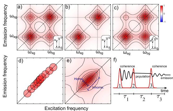
Figure 3: Example of a 2D spectra of a system with two excited levels $|a\rangle$, $|b\rangle$ and a ground state $|g\rangle$. (a) The instensity spectrum is symmetric along the diagonal since the states share a common ground, (b) the states are decoupled, (c) coupling of the $|b\rangle$ and $|a\rangle$ leads to relaxation of $|b\rangle$ towards $|a\rangle$, which translates to an asymmetric amplitude of the off-diagonal peaks. Insets in (a-c) show the energy diagrams for corresponding mechanisms and the transition frequencies are labelled by $\omega$’s. (d-e) indicate the modulus of a rephasing 2D spectrum for an inhomogeneous system that consists of a collection of emitters, where, in (d) each resonant frequency is decoupled from the others and is schematically represented by a red circle. The homogeneous width of each emitter, represented by the size of the circle, is measurable along the anti-diagonal. (e) The total signal forms an elongated peak along the diagonal (inhomogeneous broadening). (f) Pulse sequence used to perform a multi-dimensional coherence spectroscopic measurement for obtaining 3rd order polarization response.

Our approach allows one to easily compute the quantum dynamics associated with an arbitrary Hamiltonian using QuTip (v4) quantum optics package. [9] The QuTip package is robust, easy to use, and has developed a sizable user group spanning multiple areas of atomic and molecular physics. We also incorporate a symbolic approach for determining the irreducible/non-vanishing double-sided Feynman diagrams  [10], which provides a straight-forward way to compute the 2D responses in the time-domain. Additionally, our method leverages the efficient Fast-Fourier Transform (FFT) capabilities in Numpy for efficient conversions to frequency domain. Lastly, we note that our approach is not limited to 3rd order non-linear responses. In principle, one can use our approach to simulate arbitrary order experiments with arbitrarily complicated system/bath Hamiltonians, limited only by the computational resources (and time) available to the user.

The disadvantage of our current implementation is that it assumes the interaction with the external laser field is purely impulsive, acting only at a single instant in time. However, this is not an extreme limitation since the experimental setups we are most interested in studying, achieve this limit using temporally narrow pulses that span the entire spectral frequency range of the system. Additionally, the pulse overlap is often an experimentally undesirable situation that results in coherence spikes and inclusion of additional diagrams in the signal of interest, a situation most experiments tend to avoid. [10, 21] Finally, it is fairly straight-forward to implement finite-sized pulses within our approach and we reserve this for a future release of our method.

3 Downloading and installation

QuDPy relies on only a few packages namely QuTip for quantum dynamics, UFSS for diagram generation, and supporting packages such as NumPy and Matplotlib. The QuDPy package can be installed with simple command pip install qudpy==1.x.x where 1.x.x is the version number. The installation process installs any required packages automatically in case they are currently not installed. The online github repository for the package can be found here (https://github.com/sa-shah/QuDPy).

QuDPy itself is composed of two subroutines i.e. Classes and plot_functions. The structure of program is shown in Figure 4. The details of methods and functions available in the package (along with their input and output parameters) are provided in the Appendix.

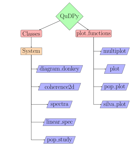
Figure 4: QuDPy structure, the subroutines are shown in red, and the functions are shown in purple.

4 Example Calculations

Before giving two worked examples, we give an overview of the typical workflow for using our approach. This section does not provide the complete code as it is documented in the Example 1 and 2 available on Google Colab (links available on the frontpage).

4.1 Typical Workflow

A typical work-flow using our approach begins by first defining the system Hamiltonian using the QuTip package and then initializing the diagram-generation code in UFSS using a desired phase-matching/phase-cycling condition.[10, 11] The diagram-generation step is formally agnostic of the system Hamiltonian at this point and these two initial steps can be easily swapped. Furthermore, the user can provide custom diagrams without invoking UFSS, provided the diagrams are in the format required by the UFSS routine.

The system-setup can be accomplished using the System() command provided in the QuDPy package e.g. a custom system with Hamiltonian Hd, light-matter interaction operator A, dipole operator mud, collapse operator list c_ops and density matrix rho, can be created by

⬇

sys=System(H=Hd,

a=A,

u=mud,

c_ops=[c1d,c2d,c3d,c4d],

rho=rho)

This is provided as utility routine for setting up the system and its associate quantum Fock space (that depends on the basis used to define Hamiltonian and interaction operator). We next provide two worked examples to illustrate how to use our code for performing spectral simulations.

4.1.1 Inclusion of light-matter interaction in quantum evolution

In addition to the evolution under system bath interaction, the system also observes light-matter interaction in accordance with a given double-sided diagram. The diagram is generated by the Automatic Diagram Generator in UFSS for given phase-matching or phase-cycling conditions. For example, consider the case of $R^{(3)}_{1,2,3}$ in the phase matching direction $-k_{1}+k_{2}+k_{3}$; the corresponding diagrams can be generated by:

⬇

import ufss

R3rd = ufss.DiagramGenerator()

R3rd.set_phase_discrimination([(0,1),(1,0),(1,0)])

d = np.array([1]) # assigning pulse durations

R3rd.efield_times = [d, d, d, d]

# setting pulse delays

time_ordered_diagrams_rephasing = R3rd.get_diagrams([0,100,200,200])

[R3, R1, R2] = time_ordered_diagrams_rephasing

rephasing = [R1, R2, R3]

In the code above, each pulse is considered 1 fs long with pulse delays $t_{1},t_{2},t_{3}$ of $100,200$, and $200$ fs, respectively (Note: these delays are arbitrary at this point and selected only to ensure non-overlapping pulses). The double-sided diagrams are contained in $R1,R2$, and $R3$. These diagrams then become inputs for calculating the spectral response with appropriate system evolution.

4.1.2 Imposing time gating for light matter interactions

Given a system and a double-sided diagram, the density matrix evolves with the appropriate master equation until a light-matter interaction is encountered as dictated by the diagram. At this time, the corresponding raising or lower operation is applied from the left or right on the density matrix. Afterwards, the density matrix becomes the initial density matrix for the next step of evolution under the same master equation as before till the next light-matter interaction. This patterns is repeated for all light-matter interactions. For experimentally observable spectroscopic response, only the final state after last light-matter interaction is of importance; however, states throughout the evolution can be saved for inspection.

4.1.3 2D Coherence

In a particularly useful experimental scheme, the coherence generated under different light-matter interactions in a double-sided diagram is utilized to probe intra-material interactions spectroscopically. In this approach, two time delays are tuned, while all others are kept fixed. The resulting final density matrices are used to generate 2D spectra by computing $\langle\mu\rangle$. The scan range for adjustable time delays is determined by either experimental feasibility or the desired spectroscopic frequency precision.

For example in $R_{1}$, coherences are generated during time intervals $t_{1}$ and $t_{3}$ (i.e. $|0\rangle\langle 1|$ and $|1\rangle\langle 0|$). The set of final states in corresponding 2D coherence with a $t_{1}$ and $t_{3}$ range of 200 fs each and $t_{2}$ fixed at 20 fs, can be generated by

⬇

sys1 = System().

t1, t2, t3 = (200, 20, 200)

statesR1 = sys1.response2D_pop(R1, t1, t2, t3)

These can then be used to generate spectra with in-built functions which simply compute $\langle\mu\rangle$ from these states.

4.2 Fourier Transform and Resolution in Frequency Domain

To generate high-resolution 2D coherence spectra, follow these guidelines for efficient utilization of computational resources:

• Increase time-domain resolution for a larger scanned frequency range in the spectra.

• Use the maximum difference between eigenvalues of the system Hamiltonian to estimate the minimum time-step via Nyquist theorem for a faithful simulation. Note, the step size must be small enough to support QuTip differential equation solvers (QuTip will output an appropriate warning otherwise).

• Select a large scan-range for time-domain for improved frequency domain resolution.

• If the system loses coherence quickly, avoid additional system evolution as it would only result in smoothing of spectral features. Instead, use smoothing functions while plotting the spectra.

• For inspection of system evolution and expectation values of important observables, utilize the diagram_donkey test run before committing to a full-scale simulation.

4.3 Example 1: Excitation exchange coupling between chromophores

In the example which follows, we consider two coupled oscillators with Hamiltonian:

$$H/\hbar=\omega_{1}a^{\dagger}a+\omega_{2}b^{\dagger}b+J(a^{\dagger}b+b^{\dagger}a)$$ (14)

Physically, this corresponds to system composed of two chromophores that can exchange quanta via the exchange coupling, $J$, which can be either positive or negative. The transition dipole operator is the sum of the dipole operators for each oscillator,

$$\hat{\mu}=\mu_{A}(a+a^{\dagger})+\mu_{B}(b+b^{\dagger}).$$ (15)

In this example, we also assume each oscillator is coupled to a thermal bath which relaxes each to a thermal population. This is a general model for a wide-range of systems encountered in chemical physics.

The complete Python code for this model is provided in the Example 1 Jupyter notebooks on Google Colab.

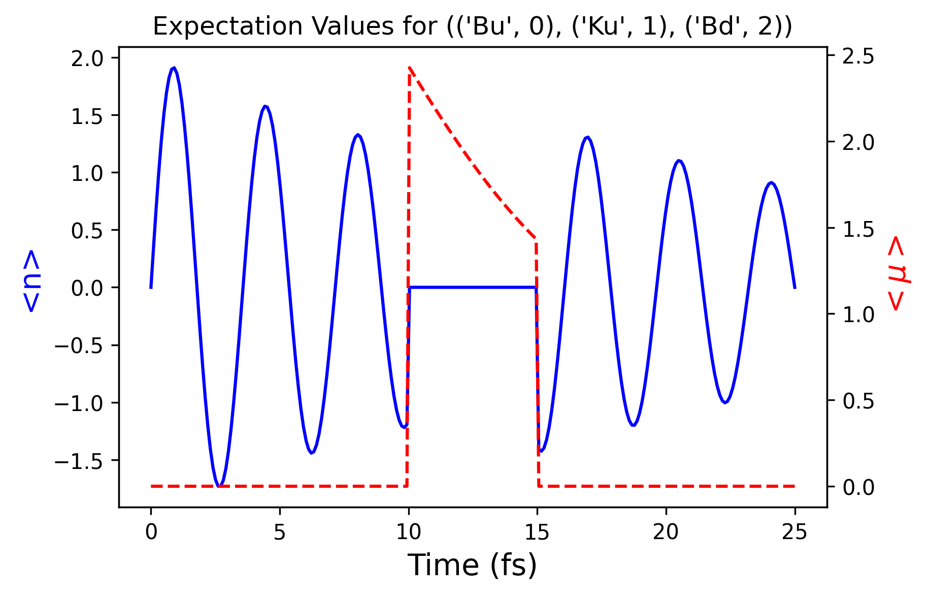
Figure 5: Results from diagram_donkey show the expectation values of system dipole (red dashed) and excitation number (blue solid) operators for a $R_{1}$ diagram with a coherence time of 5 and 10 fs for the first and second coherence, and a population time of 5 fs. The results reveal the population relaxation and loss of coherence from system-bath interactions

Once the system has been setup, we are ready to compute something and it is useful to examine the populations and coherences produced by the $R_{1}$ diagram.

⬇

states = sys.diagram_donkey([0,5,10,20],[R1],r=10)

The pulse arrival times of $0,5,10,20$ fs along with a resolution of 10 steps per fs, are selected arbitrarily to illustrate the functionality. This produces a plot showing the populations and coherences versus time as shown in Fig. 5. Notice that from time $t=0$ to 5 fs, the system evolves as a coherence $|0\rangle\langle 1|$, from 5 fs to 10 fs, the system is projected onto a population $|1\rangle\langle 1|$ where it undergoes non-radiative relaxation. As noted above, this time period is referred to as the population time. At 10 fs, it is again projected onto a coherence, this time $|1\rangle\langle 0|$ where it evolves for an additional 10fs before being projected back down to the $|0\rangle\langle 0|$ ground state. It is important to note that the coherences and populations are in the eigenbasis and not with regards to the primitive (pre-diagonalized) system.

A full simulation will involve independently scanning $t_{1}$ and $t_{3}$ for a fixed $t_{2}$ population time. This is accomplished using coherence2d() routine as illustrated here.

⬇

time_delays = [100, 5, 100]

scan_id = [0, 2]

response_list = []

states, t1, t2, dipole = sys.coherence2d(

time_delays, diagram, scan_id)

response_list.append(np.imag(dipole))

Here, we are first passing a series of time-delays $t_{1}$, $t_{2}$, and $t_{3}$, a list of diagrams, and the indices of time delays that will be scanned e.g. 0 and 2 in this case. Further options include the adjustment of temporal resolution for simulation and the use of parallel computing (if available); however, for clarity they are omitted from current example. The selection of scan range in this example, although arbitrary, is typical of ultrafast femtosecton experiments but it can be adjusted to the desired theoretical and practical requirements. This step typically requires the most computational effort since we repeat the time propagation to cover the specified temporal range with a fine-enough grid of points to resolve the spectral features. The calculations return, among other things, a 2D list of dipole operator expectation values for every choice of $t_{1}$ and $t_{3}$. This response list is the main ingredient required for calculating the observable spectra. We can now analyze the calculations and compute the 2D spectra using the spectra() function as follows:

⬇

spectra_list, extent, f1, f2 = sys.spectra(response_list)

Figure  6 displays the 2D spectra for a given $t_{2}$ population time for this example. The Fourier transform routine will return the full frequency ranging spanning both positive and negative frequencies, however, in the plots only the fourth and first quadrant are shown for rephasing and nonrephasing signals respectively. Furthermore the $y$-axis is inverted for the rephasing diagrams following the conventions of ultrafast spectroscopy.

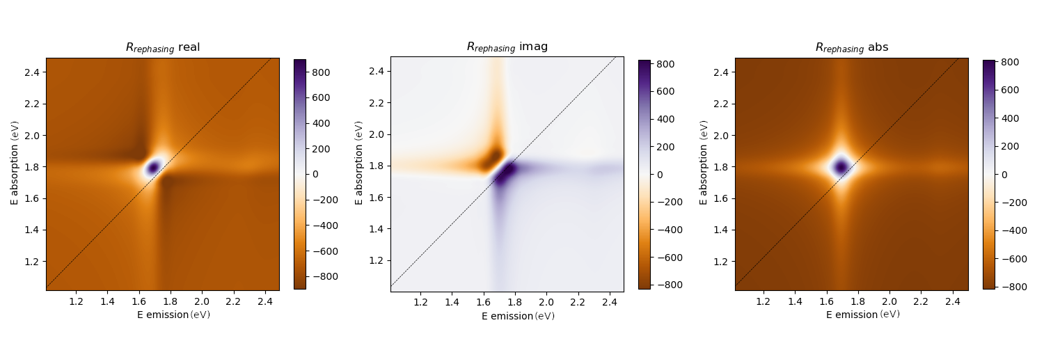
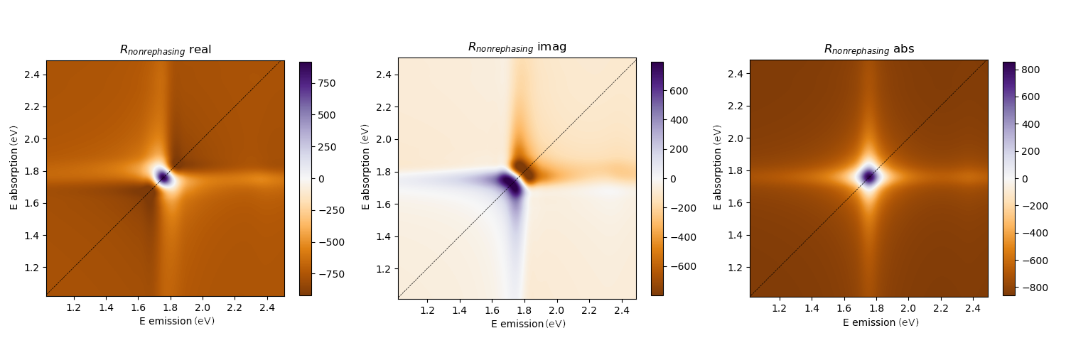
Figure 6: Frequency domain response (i.e. spectra) for two-time correlation. Top row displays the sum of rephasing diagrams $R_{1}$, $R_{2}$, and $R_{3}$ with left, center and right plots showing real, imaginary and absolute values, respectively. The bottom row represents the same for the sum of nonrephasing diagrams $R_{4}$, $R_{5}$ and $R_{6}$. These spectra only show first quadrant for the non-rephasing and fourth quandrant for rephasing (with an additional inversion of $y$-axis for rephasing).

4.4 Example 2: Cavity QED using QuDPy

In this example we consider a driven/dissipative open quantum system consisting of a finite number of independent two-state atoms coupled to a quantized mode of the radiation field (Dicke model)[22]. The Dicke model shows a mean-field phase transition to a super-radiant phase when the coupling between the light and matter crosses a critical value. The Dicke transition belongs to the Ising universality class and has been used to model a number of cavity quantum electrodynamics experiments. [23, 24, 25] While Dicke superradiant transition is analogous with the lasing instability, lasing and Dicke superradiance belong to different universality classes.[26]

In this example, we shall assume that an open-quantum system consisting of a single cavity mode coupled to $N$ independent 2-level systems is probed by an external laser field. The Hamiltonian for the model reads

$$H=\hbar\Omega_{c}a^{\dagger}a+\hbar\sum_{j=1}^{N}\omega_{j}\sigma_{z}(j)+\frac{2\lambda}{\sqrt{N}}(a+a^{\dagger})\sum_{j}\sigma_{x}(j)$$ (16)

where $\Omega_{c}$ is the frequency of the (cavity) mode and $\{\omega_{j}\}$ are the transition frequencies of the individual spins, and $\lambda$ parameterises the coupling strength between spins and cavity mode. In our worked model, we take all the spins to be identical. Under this assumption, we can define the total spin operators

$$S_{\alpha}=\sum_{j}\sigma_{\alpha}(j)$$ (17)

which satisfies the spin algebra $[S_{x},S_{y}]=i\hbar S_{z}$. Using these operators, the Hamiltonian simplifies to

$$H=\hbar\Omega_{c}a^{\dagger}a+\hbar\omega S_{z}+\frac{2\lambda}{\sqrt{N}}(a+a^{\dagger})S_{x}$$ (18)

This simplifies the numerical studies by reducing the Hilbert space for the spins from $2^{N}$ to $2S+1$ with $S\leq N/2$. Lastly, the third term is the coupling between the cavity mode and the two-level systems. The $\sqrt{N}$ is introduced so that the coupling becomes a constant in the limit of $N\to\infty$. As such, we define the coupling

$$g=\frac{2\lambda}{\sqrt{N}}$$ (19)

and write the system Hamiltonian as

$$H/\hbar=\Omega_{c}a^{\dagger}a+\omega S_{z}+g(a+a^{\dagger})S_{x}$$ (20)

In these units, the critical coupling occurs at $g_{c}=\sqrt{\Omega_{c}\omega}/2$. The Dicke model itself is related to a number of other models in quantum optics. Specifically, when $N=1$, it is the Rabi model. If the counter-rotating terms ($a\sigma^{-}(j)$ and $a^{\dagger}\sigma^{+}(j)$) are excluded, the model is termed the Jaynes-Cummings model for $N=1$ and the Tavis-Cummings model for $N>1$.

In this example, we consider the driven/dissipative Dicke model in which the density matrix evolves according to the quantum master equation

$$\frac{d}{dt}\rho=\frac{1}{i\hbar}[H,\rho]+\sum_{\alpha}\gamma_{\alpha}\left(L_{\alpha}\rho L^{\dagger}_{\alpha}-\frac{1}{2}\left\{L_{\alpha}^{\dagger}L_{\alpha},\rho\right\}\right)$$ (21)

in which we include terms for cavity decay and pumping, atomic relaxation, atomic dephasing, and collective decay. Our simulations are initialized by first requiring the density matrix of the system to be in a steady-state with regards to the unperturbed quantum master equation, i.e. $d\rho_{ss}/dt=0$. Once $\rho_{ss}=\rho(-\infty)$ has been determined, either via numerical relaxation or analytically, the simulation proceeds as above. For this we assume a thermal population of photons in the cavity mode (as determined by the pumping intensity) and define Lindblad operators

$$L_{1}=\sqrt{\kappa(n_{th}+1)}a$$ (22)

$$L_{2}=\sqrt{\kappa n_{th}}a^{\dagger}$$ (23)

where $\kappa$ is the photon exchange rate between the cavity mode and the external bath.

Within our model, we assume that the driven/dissipative cavity+spins system is additionally probed by a series of perturbative ultrafast pulses that exchange quanta with the cavity mode via

$$H_{cav/laser}\propto\mu_{cav}(b^{\dagger}_{laser}a+a^{\dagger}b_{laser}).$$ (24)

Taking the applied laser-field to be semi-classical, we can write this as

$$H_{cav/laser}\propto\mu_{cav}(E(t)a+E^{*}(t)a^{\dagger})$$ (25)

where $E(t)$ is the electric field of the applied probe pulses and $\mu_{cav}$ is the transition dipole of the cavity. This assumption is based upon the fact that the experimental signals correspond to the macroscopic polarizability of the entire cavity system. Figure 7 provides a pictorial representation of the proposed experiment.

Figure 7: Dicke Model system for third order response. The cavity contains two-level systems (TLS) which interact with each other and the cavity mode (represented by red curve). The cavity itself is pumped with an incoherent light source (bulb) and the whole system is probed with two pulses $K_{1}$ and $K_{2}$ . The generated signal in a proper phase-matching direction is shown as $K_{signal}$.

In our examples we consider the non-linear 3rd order response for a resonant cavity $\hbar\Omega_{c}=\hbar\omega_{j}=1$ which has a critical coupling of $\lambda_{c}=\frac{\sqrt{\Omega_{c}\omega}}{2}=1/2$. The simulation is performed with a cavity-spin coupling strength of $0.25$, $N=6$ spins and 6-state basis for the cavity mode. The cavity pumping/relaxation rate $\kappa$ is set at $0.05$. Additionally, the spin dephasing is introduced as $\sqrt{0.15}S_{z}$. These are chosen as model parameters and are not specific to particular physical system. The detailed list of parameters and additional information is provided in the relevant Jupyter notebooks in the SI/github repository.

Fig. 8 shows the predicted 2D coherence spectra for our model system. In this case, one can clearly see symmetric off-diagonal coherences between the two diagonal peaks corresponding to the lower and upper polariton (LP and UP) states of this system. In this case, both LP and UP are connected to a common ground-state. Physically, this can be understood since in setting up the problem we transformed the cavity operators $a$ and $a^{\dagger}$ to the eigenbasis of the Dicke Hamiltonian. More complex dynamics can be introduced (for example) by including incoherent relaxation pathways via additional Lindblad operators.

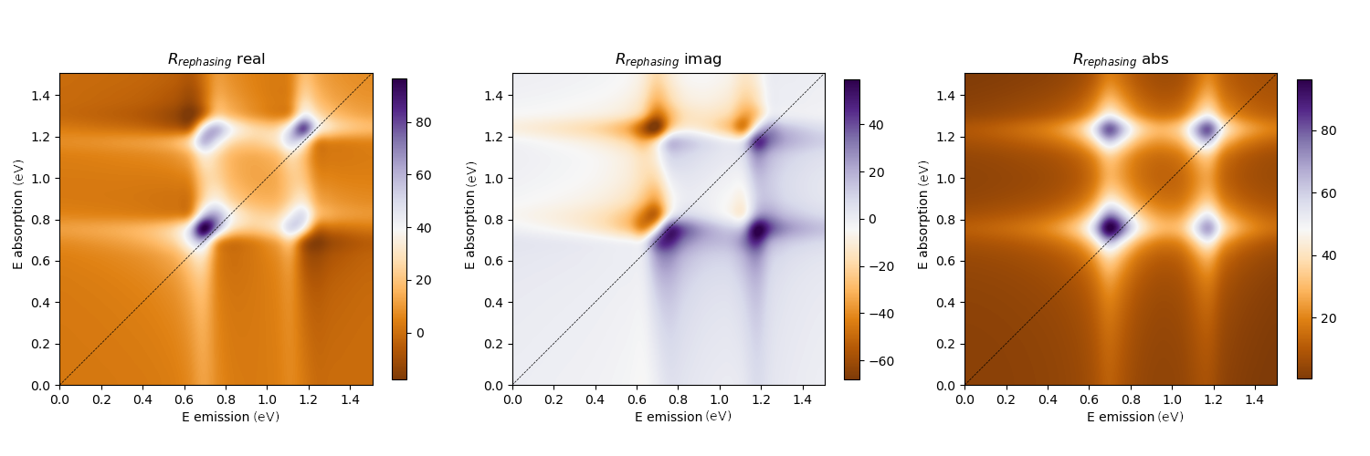
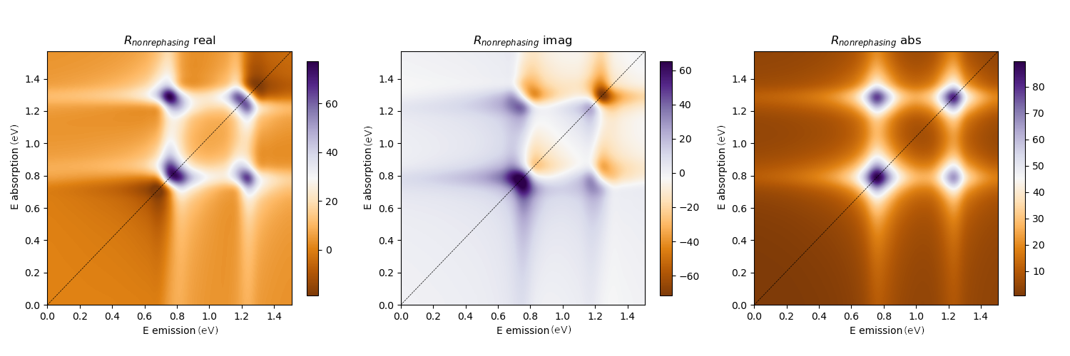
Figure 8: 2D coherence spectra of response for example 2. Top row displays the sum of rephasing diagrams $R_{1}$, $R_{2}$, and $R_{3}$ and the bottom row represents the same for the sum of nonrephasing diagrams $R_{4}$, $R_{5}$ and $R_{6}$. The left, center and right columns show real, imaginary and absolute values, respectively. Only first quadrant for the non-rephasing and fourth quandrant for rephasing diagrams are shown.

5 Discussion

We present here the first-release of our generalized package for simulating non-linear spectral responses observed in modern ultrafast spectroscopy. While our examples have focused upon optical signals, the approach we have adopted can be used to model a wide-range of physical problems with significant ease and control allowing the end-user to rapidly create model Hamiltonian systems and compute accurate responses. We have avoided a detailed analysis of the results to keep the discussion focused on introducing the package and its use. Future releases of this code will include the facility for more complex pulse-shapes, time-dependent system Hamiltonians, electric field polarization, and the means to connect the approach to ab-initio and molecular dynamics treatments of molecular systems that can provide an explicit Hamiltonian with excitation manifolds and inter-band transition dipoles (as QuTip is capable of simulating the appropreate quantum dyanmics provided the explicit Hamiltonian). We believe that the code will have tremendous utility within the ultrafast spectroscopy user community as well as a useful pedagogic tool for courses on modern spectroscopic methods.

Author Contributions:

S. A. Shah: Conceptualization, Methodology, Formal analysis, Visualization, Writing - Original draft. Hao Li: Formal analysis. Eric R. Bittner: Conceptualization, Methodology, Project administration, Writing - Review & Editing, Funding acquisition, Supervision. Carlos Silva: Conceptualization,Project administration, Funding acquisition. Andrei Piryatinski: Conceptualization, Funding acquisition, Formal analysis.

Appendix A Functions and Methods

The default System class variables are as follows

• $\hbar=0.658211951$ in eV fs.

• $\omega$, system frequency with a default value of $E/\hbar$ with $E=2$ eV.

• $H$, Hamiltonian with default value of $\hbar\omega a^{\dagger}a$

• $a$, the system lowering operator for light-matter interaction. By default it is the lowering operator of a 3-level harmonic oscillator.

• $\mu$, the system dipole operator. Default value is $\mu=a^{\dagger}+a$

• $c\_ops$, a list of collapse operators for Lindblad simulation. By defaults its empty.

Furthermore, the System class can be initialized with following values.

• n, total energy levels.

• H, Hamiltonian

• rho, initial density matrix

• a, system lowering operator encoding emission of photon.

• u, system dipole operator defined as $\mu(a^{\dagger}+a)$. $\mu=1$ typically.

• c_ops, list of collapse operators encoding system-bath coupling.

• e_ops (optional), list of operators for which expectation values are demanded in each simulation. Typically and empty list.

• tlist (optional), list of time steps for simulation. Typically not required during system initialization.

• diagonalize, True/False can perform Hamiltonian diagonalization and basis transformation of all operators if required.

A.1 Functions

The following functions are contained in System class subroutine (see Figure 4 for hierarchy details.

• diagram_donkey, for simulating a single trial of system

• coherence2d, for generating two-time coherence response.

• spectra, for converting the temporal response to spectra.

• linear_spectra, for calculating and generating a linear

• pop_study, for computing a series of 2D-coherence

Similarly the plot_functions subroutine contains the following functions,

• multiplot, for plotting multiple response (temporal or frequency) simultaneously.

• plot, for single spectrum or temporal response

• pop_plot, for plotting a response on multiple population times.

A.1.1 diagram_donkey

Computes and plots a single evolution of the density matrix for a list of double-sided diagrams. Mainly useful for inspection/instructional purposes. Inputs:

• interaction_times (required), a list of arrival times for pulses and the last entry is time interval for detection of local oscillator.

• diagrams(required), a list of double-sided diagrams in UFSS diagramGenerator format.

• r (optional), temporal resolution (time steps per fs)

Outputs:

None, just plots the diagram.

Notes:

First pulse arrives at t=0.

A.1.2 coherence2d

Computes the 2D coherence plot for a single diagram with only two scan-able delays. It can be parallelized if resources are available.

Inputs:

• time_delays (required), list of time delays. Provide time delay for each interaction even if zero. Default is None. These should be guided by experimental and theoretical considerations for each user.

• diagram (required), a double-sided diagram in UFSS diagramGenerator format. Default is None. Utilize desired phase-matching/phase-cycling conditions for diagram generation.

• scan_id (required), a list of indices for the time delays in interaction_times that have to be scanned. Default is None

• r (optional), time resolution of simulation in steps per fs. Default value is 10. Should be guided by the energy eigenvalues of desired Hamiltonian.

• parallel (optional), parallelization control, True or False. Default is False

Outputs:

• A 2D list of density matrices for each pair of scanned times.

• A numpy array of first scan time

• A numpy array of second scan time

• A 2D list of $\langle\mu\rangle$

Notes:

A.1.3 spectra

Converts the list of dipoles into spectra though Fourier transform.

Inputs:

• dipoles (required), a list of dipoles. Default is None

• resolution (optional), time resolution. Default is 10 steps per fs.

Outputs:

• List of spectra

• Minimum and maximum limits of each frequency axis

• grid of first frequency

• grid of second frequency

Notes:

A.1.4 linear_spec

For computing simple linear spectra from the system after any number of interaction in the start.

Inputs:

• scan_time (required), time interval to be simulated in fs.

• diagram (optional), double-sided diagram for calculating the system response. All interactions contained in the diagram are applied at t=0. If diagram=None, then by default a ’Bu’ interaction is applied at t=0.

• resolution (optional), time resolution of simulation in steps per fs.

Outputs:

• dipole expectation value

• time

• spectrum

• frequency

Notes:

For increasing the frequency resolution, simply increase the scan_time. For decreasing the range of frequencies, decrease the time resolution.

The function also plots the spectrum.

A.1.5 pop_study

For calculating the nonlinear response of a double-sided diagram for a set of population times.

Inputs:

• pop_time_list (required), a list of population times. Default None

• pop_index (required), an index of the population generating interaction. Default 1.

• time_delays (required), a list of time delays between interactions. Default None

• diagram (required), a double-sided diagram to be simulated. Default None

• scan_id (required), list of indices of time delays to be scanned for 2D coherence plot. Default None.

• r (optional), time resolution of simulation in steps per fs. Default is 10.

• parallel (optional), a True/False control of parallelized computation. Default is False

Outputs:

• list of 2D coherence response for each population time

• First scan time list

• Second scan time list

• List of spectra for each population time

• Extent of x and y-axis in spectra

• First frequency grid for spectra

• Second frequency grid for spectra.

Notes:

A.1.6 multiplot

Plot multiple data sets for spectral and evolution data.

Inputs:

• data (required), a list of spectra or dipole expectation values or any other variable of interest. Default None

• scan_range (required), the min and max of both axis in the format [xmin, xmax, ymin, ymax]. Default None

• labels (required), a list of label for each axis. Default None

• title_list (required), a List of titles for each plot. Default None

• scale (optional), scaling of the data points, two choices are ’linear’ and ’log’. Default ‘linear’.

• color_map(optional), choice of colormap. Default ‘viridis’.

• interpolation (optional), interpolation for points in plot. Default ‘spline36’. Can be changed to None

Outputs:

Does not return any output, only generates the plots.

Notes:

A.1.7 plot

Plots a single data set.

Inputs:

• data (required), a spectrum or dipole expectation value list or any other variable of interest. Default None

• scan_range (required), the min and max of both axis in the format [xmin, xmax, ymin, ymax]. Default None

• label (required), a list of label for each axis. Default None

• title_list (required), a title for plot. Default None

• scale (optional), scaling of the data points, two choices are ’linear’ and ’log’. Default ‘linear’.

• color_map(optional), choice of colormap. Default ‘viridis’.

• interpolation (optional), interpolation for points in plot. Default ‘spline36’. Can be changed to None

Outputs:

Does not return any output, only generates the plot.

Notes:

A.1.8 pop_plot

Same as multiplot as of now. Will be updated in future.

A.1.9 silva_plot

Plot multiple data sets for spectral and evolution data.

Inputs:

• spectra_list (required), a list of spectra or dipole expectation values or any other variable of interest. Default None

• scan_range (required), the min and max of both axis in the format [xmin, xmax, ymin, ymax]. Default None

• labels (required), a list of label for each axis. Default None

• title_list (required), a List of titles for each plot. Default None

• scale (optional), scaling of the data points, two choices are ’linear’ and ’log’. Default ‘linear’.

• color_map(optional), choice of colormap. Default ‘PuOr’.

• interpolation (optional), interpolation for points in plot. Default ‘spline36’. Can be changed to None.

• center_scale (optional), control for centering each data set in the list around zero by simple scale shift. default value is True.

• plot_sum (optional), control for generating and plotting the total spectrum from the input list by summation of individual data sets. Default True.

• plot_quadrant (optional), select a particular quadrant for the plot. Possible values are ‘1’, ‘2’, ‘3’ and ‘4’. Default is ‘All’

• invert_y (optional), control for inverting y-axis by changing negative values to positive. Default is False

• diagonals (optional), list of True/False values for including (or excluding) the diagonal and cross diagonal reference lines. The default is [True, True]

Outputs:

Does not return any output, only generates the plots.

Notes:

References

- [1] S. Mukamel, Principles of Nonlinear Optics and Spectroscopy, Oxford University Press, 1995.
- [2] P. Hamm, M. Zanni, Concepts and Methods of 2D Infrared Spectroscopy, Cambridge University Press, (2011).
- [3] Peter A. Rose and Jacob J. Krich, Automatic Feynman diagram generation for nonlinear optical spectroscopies and application to fifth-order spectroscopy with pulse overlaps, J. Chem. Phys. 154, 034109 (2021).
- [4] J. Johansson, P. Nation, F. Nori, Qutip 2: A python framework for the dynamics of open quantum systems, Computer Physics Communications 184 (4) 1234–1240, (2013)

References

-
[1]
F. D. Fuller, J. P. Ogilvie,
Experimental
implementations of two-dimensional Fourier transform electronic
spectroscopy, Annual Review of Physical Chemistry 66 (1) (2015) 667–690,
pMID: 25664841.
arXiv:https://doi.org/10.1146/annurev-physchem-040513-103623, doi:10.1146/annurev-physchem-040513-103623.
URL https://doi.org/10.1146/annurev-physchem-040513-103623 -
[2]
A. R. Srimath Kandada, H. Li, E. R. Bittner, C. Silva-Acuña,
Homogeneous optical line
widths in hybrid Ruddlesden–Popper metal halides can only be measured using
nonlinear spectroscopy, The Journal of Physical Chemistry C 126 (12) (2022)
5378–5387.
arXiv:https://doi.org/10.1021/acs.jpcc.2c00658, doi:10.1021/acs.jpcc.2c00658.
URL https://doi.org/10.1021/acs.jpcc.2c00658 -
[3]
J. P. Ogilvie, K. J. Kubarych,
Chapter
5 multidimensional electronic and vibrational spectroscopy: An ultrafast
probe of molecular relaxation and reaction dynamics, in: Advances in Atomic
Molecular and Optical Physics, Vol. 57 of Advances In Atomic, Molecular, and
Optical Physics, Academic Press, 2009, pp. 249–321.
doi:https://doi.org/10.1016/S1049-250X(09)57005-X.
URL https://www.sciencedirect.com/science/article/pii/S1049250X0957005X -
[4]
S. Mukamel,
Multidimensional
femtosecond correlation spectroscopies of electronic and vibrational
excitations, Annual Review of Physical Chemistry 51 (1) (2000) 691–729,
pMID: 11031297.
arXiv:https://doi.org/10.1146/annurev.physchem.51.1.691, doi:10.1146/annurev.physchem.51.1.691.
URL https://doi.org/10.1146/annurev.physchem.51.1.691 -
[5]
D. M. Jonas,
Two-dimensional
femtosecond spectroscopy, Annual Review of Physical Chemistry 54 (1) (2003)
425–463, pMID: 12626736.
arXiv:https://doi.org/10.1146/annurev.physchem.54.011002.103907,
doi:10.1146/annurev.physchem.54.011002.103907.https://www.overleaf.com/project/626186811b799a3fe13999f8
URL https://doi.org/10.1146/annurev.physchem.54.011002.103907 -
[6]
M. Maiuri, M. Garavelli, G. Cerullo,
Ultrafast spectroscopy: State of
the art and open challenges, Journal of the American Chemical Society
142 (1) (2020) 3–15, pMID: 31800225.
arXiv:https://doi.org/10.1021/jacs.9b10533, doi:10.1021/jacs.9b10533.
URL https://doi.org/10.1021/jacs.9b10533 - [7] S. Mukamel, Principles of Nonlinear Optics and Spectroscopy, Oxford University Press, 1995.
- [8] P. Hamm, M. Zanni, Concepts and Methods of 2D Infrared Spectroscopy, Cambridge University Press, 2011. doi:10.1017/CBO9780511675935.
-
[9]
J. Johansson, P. Nation, F. Nori,
Qutip
2: A python framework for the dynamics of open quantum systems, Computer
Physics Communications 184 (4) (2013) 1234–1240.
doi:https://doi.org/10.1016/j.cpc.2012.11.019.
URL https://www.sciencedirect.com/science/article/pii/S0010465512003955 -
[10]
P. A. Rose, J. J. Krich, Automatic
feynman diagram generation for nonlinear optical spectroscopies and
application to fifth-order spectroscopy with pulse overlaps, The Journal of
Chemical Physics 154 (3) (2021) 034109.
arXiv:https://doi.org/10.1063/5.0024105, doi:10.1063/5.0024105.
URL https://doi.org/10.1063/5.0024105 -
[11]
P. A. Rose, J. J. Krich, Efficient
numerical method for predicting nonlinear optical spectroscopies of open
systems, The Journal of Chemical Physics 154 (3) (2021) 034108.
arXiv:https://doi.org/10.1063/5.0024104, doi:10.1063/5.0024104.
URL https://doi.org/10.1063/5.0024104 -
[12]
Wei Zhuang, Darius Abramavicius, Tomoyuki Hayashi, and Shaul Mukamel, Simulation Protocols for Coherent Femtosecond Vibrational Spectra of Peptides, J. Phys. Chem. B 2006, 110, 7, 3362–3374.
https://doi.org/10.1021/jp055813u.
URL https://pubs.acs.org/doi/10.1021/jp055813u -
[13]
P. F. Tekavec, G. A. Lott, A. H. Marcus,
Fluorescence-detected
two-dimensional electronic coherence spectroscopy by acousto-optic phase
modulation, The Journal of Chemical Physics 127 (21) (2007) 214307.
arXiv:https://doi.org/10.1063/1.2800560, doi:10.1063/1.2800560.
URL https://doi.org/10.1063/1.2800560 -
[14]
K. J. Karki, J. R. Widom, J. Seibt, I. Moody, M. C. Lonergan, T. Pullerits,
A. H. Marcus, Coherent
two-dimensional photocurrent spectroscopy in a pbs quantum dot photocell,
Nature Communications 5 (1) (2014) 5869.
doi:10.1038/ncomms6869.
URL https://doi.org/10.1038/ncomms6869 -
[15]
A. A. Bakulin, C. Silva, E. Vella,
Ultrafast spectroscopy
with photocurrent detection: Watching excitonic optoelectronic systems at
work, The Journal of Physical Chemistry Letters 7 (2) (2016) 250–258.
doi:10.1021/acs.jpclett.5b01955.
URL https://doi.org/10.1021/acs.jpclett.5b01955 -
[16]
E. Vella, H. Li, P. Grégoire, S. M. Tuladhar, M. S. Vezie, S. Few, C. M.
Bazán, J. Nelson, C. Silva-Acuña, E. R. Bittner,
Ultrafast decoherence dynamics
govern photocarrier generation efficiencies in polymer solar cells,
Scientific Reports 6 (1) (2016) 29437.
doi:10.1038/srep29437.
URL https://doi.org/10.1038/srep29437 -
[17]
H. Li, A. Gauthier-Houle, P. Grégoire, E. Vella, C. Silva-Acuña, E. R.
Bittner,
Probing
polaron excitation spectra in organic semiconductors by
photoinduced-absorption-detected two-dimensional coherent spectroscopy,
Chemical Physics 481 (2016) 281–286.
doi:https://doi.org/10.1016/j.chemphys.2016.07.004.
URL https://www.sciencedirect.com/science/article/pii/S0301010416304517 - [18] Qutip Documentation, URL https://qutip.org/docs/latest/apidoc/functions.html#
-
[19]
A. Redfield,
in: J. S. Waugh (Ed.), Advances in
Magnetic Resonance, Vol. 1 of Advances in Magnetic and Optical Resonance,
Academic Press, 1965, pp. 1–32.
doi:https://doi.org/10.1016/B978-1-4832-3114-3.50007-6.
URL https://www.sciencedirect.com/science/article/pii/B9781483231143500076 -
[20]
G. Lindblad, On the generators of
quantum dynamical semigroups, Communications in Mathematical Physics 48 (2)
(1976) 119–130.
doi:10.1007/BF01608499.
URL https://doi.org/10.1007/BF01608499 - [21] Z. Vardeny and J. Tauc, Picosecond coherence coupling in the pump and probe technique, Optics Communications, Vol 39, 6, 396-400 (1981) URL https://doi.org/10.1016/0030-4018(81)90231-5
-
[22]
R. H. Dicke, Coherence in
spontaneous radiation processes, Phys. Rev. 93 (1954) 99–110.
doi:10.1103/PhysRev.93.99.
URL https://link.aps.org/doi/10.1103/PhysRev.93.99 -
[23]
F. Dimer, B. Estienne, A. S. Parkins, H. J. Carmichael,
Proposed
realization of the dicke-model quantum phase transition in an optical cavity
QED system, Phys. Rev. A 75 (2007) 013804.
doi:10.1103/PhysRevA.75.013804.
URL https://link.aps.org/doi/10.1103/PhysRevA.75.013804 -
[24]
D. Nagy, G. Kónya, G. Szirmai, P. Domokos,,
Dicke-model
phase transition in the quantum motion of a Bose-Einstein condensate in an
optical cavity, Phys. Rev. Lett. 104 (2010) 130401.
doi:10.1103/PhysRevLett.104.130401.
URL https://link.aps.org/doi/10.1103/PhysRevLett.104.130401 -
[25]
K. Baumann, C. Guerlin, F. Brennecke, T. Esslinger,
Dicke quantum phase transition
with a superfluid gas in an optical cavity, Nature 464 (7293) (2010)
1301–1306.
doi:10.1038/nature09009.
URL https://doi.org/10.1038/nature09009 -
[26]
M. M. Roses, E. G. Dalla Torre,
Dicke model, PLOS ONE
15 (9) (2020) 1–8.
doi:10.1371/journal.pone.0235197.
URL https://doi.org/10.1371/journal.pone.0235197