Differential Privacy has Bounded Impact on Fairness in Classification

Abstract

We theoretically study the impact of differential privacy on fairness in classification. We prove that, given a class of models, popular group fairness measures are pointwise Lipschitz-continuous with respect to the parameters of the model. This result is a consequence of a more general statement on accuracy conditioned on an arbitrary event (such as membership to a sensitive group), which may be of independent interest. We use this Lipschitz property to prove a non-asymptotic bound showing that, as the number of samples increases, the fairness level of private models gets closer to the one of their non-private counterparts. This bound also highlights the importance of the confidence margin of a model on the disparate impact of differential privacy.

autotabularcenter/.style= file=#1, after head= , table head= , late after line= , table foot= , late after last line= , command=, autobooktabularcenter/.style= file=#1, after head= , table head=   , late after line= , table foot= , late after last line= , command=,

1 Introduction

The performance of machine learning models have mainly been evaluated in terms of utility, that is their ability to solve specific tasks. However, they can be used in sensitive contexts, and impact people’s lives. It is thus crucial that users can trust these models. While trustworthiness encompasses multiple concepts, fairness and privacy have attracted a lot of interest in the past few years. Fairness requires models not to unjustly discriminate against specific individuals or subgroups of the population, and privacy preserves individual-level information about the training data from being inferred from the model. These two notions have been extensively studied in isolation: there exists numerous approaches to learn fair models (Caton & Haas, 2020; Mehrabi et al., 2021), or to preserve privacy (Dwork et al., 2014; Liu et al., 2021). However, only few works studied the interplay between privacy and fairness. In this paper, we take a step forward in this direction, proposing a new theoretical bound on the relative impact of privacy on fairness in classification.

Fairness takes various forms (depending on the task and context), and several definitions exist. On the one hand, the goal may be to ensure that similar individuals are treated similarly. This is captured by individual fairness (Dwork et al., 2012) and counterfactual fairness (Kusner et al., 2017). On the other hand, group fairness requires that decisions made by machine learning models do not unjustly discriminate against subgroups of the population. In this paper, we focus on group fairness and consider four popular definitions, namely Equalized Odds (Hardt et al., 2016), Equality of Opportunity (Hardt et al., 2016), Accuracy Parity (Zafar et al., 2017), and Demographic Parity (Calders et al., 2009).

Differential privacy (Dwork, 2006) has been widely adopted for controlling how much information the output of an algorithm may leak about its input data. It allows publishing machine learning models while preventing an adversary from guessing too confidently the presence (or absence) of an individual in the training data. To enforce differential privacy, one typically releases a noisy estimate of the true model (Dwork, 2006), so as to conceal any sensitive information contained in individual data points. This induces a trade-off between the strength of the protection and the utility of the learned model. While this trade-off has been extensively studied (Chaudhuri et al., 2011; Bassily et al., 2014; Liu et al., 2021), its implications for fairness are not yet well understood.

Contributions. In this work, we quantify the difference in fairness levels between private and non-private models in multi-class classification. We derive high probability bounds showing that this difference shrinks at a rate of $\widetilde{O}(\nicefrac{{\sqrt{p}}}{{n}})$, where $n$ is the number of data records, and $p$ the dimension of the model. To obtain this result, we first prove that the accuracy of a model conditioned on an arbitrary event (such as membership to a sensitive group), is pointwise Lipschitz continuous with respect to the model parameters. This property is inherited by many popular group fairness notions, such as Equalized Odds, Equality of Opportunity, Accuracy Parity and Demographic Parity. Consequently, two sufficiently close models will have similar fairness levels. We then upper-bound the distance between the optimal non-private model and the private models obtained with privacy preserving mechanisms like output perturbation (Chaudhuri et al., 2011; Lowy & Razaviyayn, 2021) or DP-SGD (Song et al., 2013; Bassily et al., 2014). These bounds hold for strongly convex empirical risk minimization formulations, potentially allowing explicit fairness-promoting convex regularization terms (Bechavod & Ligett, 2017; Huang & Vishnoi, 2019; Lohaus et al., 2020; Tran et al., 2021). Combining these two results, we derive high probability bounds on the fairness loss due to privacy. They show that, with enough training examples, (i) given an optimal non-private model, enforcing privacy will not harm fairness too much, and (ii) given a private model, the corresponding (unknown) non-private optimal model cannot be vastly fairer. Our results also highlight the role of the confidence margin of models in the disparate impact of differential privacy: notably, if the non-private model has high per-group confidence, then our bound on the loss in fairness due to privacy will be smaller. Our contributions can be summarized as follows:

• We prove that group fairness is pointwise Lipschitz, with a smaller constant for models with large margins.

• We bound the distance between private and optimal models, and show that the difference in their fairness levels decreases in $\widetilde{O}(\nicefrac{{\sqrt{p}}}{{n}})$.

• We show that this bound can be computed even when the optimal model is unknown, and numerically demonstrate that we obtain non-trivial guarantees.

Related work. The joint study of fairness and privacy in machine learning only goes back a few years, and has been the focus of a recent survey (Fioretto et al., 2022). One may identify three main research directions. First, it has been empirically observed that privacy can exacerbate unfairness (Bagdasaryan et al., 2019; Pujol et al., 2020; Farrand et al., 2020; Uniyal et al., 2021; Ganev et al., 2022) and, conversely, that enforcing fairness can lead to more privacy leakage for the unprivileged group (Chang & Shokri, 2020). These empirical results suggest that some properties of the dataset (such as group sizes and groupwise input norms) and the choice of the private training method may affect the extent of these disparate impacts. Unfortunately, these observations are not supported by theoretical results, and it is not clear why and when disparate impact occurs. Second, a few approaches have been proposed to learn models that are both fair and privacy preserving. However, these works either have limited theoretical guarantees on their performance (Kilbertus et al., 2018; Xu et al., 2019, 2020; Tran et al., 2020), or learn stochastic models which might not be usable in contexts where deterministic decisions are expected (Jagielski et al., 2019; Mozannar et al., 2020). Finally, a few works have shown that fairness and privacy are incompatible in some settings, in the sense that there exists data distributions where enforcing one prevents the other from being satisfied (Sanyal et al., 2022), or where enforcing both implies trivial utility (Cummings et al., 2019; Agarwal, 2020). While appealing at first glance, these results usually consider unrealistic cases that are hardly encountered in practice. In this paper, we also study fairness and privacy jointly but rather than studying whether they may be achieved simultaneously, we investigate the relative difference in fairness level between private and non-private models.

To the best of our knowledge, the work closest to ours is the one of Tran et al. (2021). They analyze the impact of privacy on fairness in Empirical Risk Minimization, where their notion of fairness is defined as the difference between the excess risk computed on the overall population and the excess risk computed on a subgroup of the population. They study the expected behavior over the possible private models while our results are model-specific. In line with our work, their results suggest that the distance to the decision boundary plays a key role in the disparate impact of differential privacy. However, the quantity appearing in their result is based on a second-order Taylor approximations which is loose for popular classification loss functions. In contrast, the quantity appearing in our bounds is precisely the confidence margin considered in prior work on multi-class margin-based classification (Cortes et al., 2013). Finally and most importantly, loss-based fairness does not necessarily imply that the actual decisions taken by the model are fair with respect to standard group-fairness notions (Lohaus et al., 2020). In contrast, our work provides guarantees in terms of these widely-accepted group fairness definitions.

2 Preliminaries

In this section, we present the fairness and privacy notions that will be used throughout the paper. We consider a multi-class classification setting with a feature space $\mathcal{X}$, a finite set of labels $\mathcal{Y}$, and a finite set $\mathcal{S}$ of values for the sensitive attribute. Let $\mathcal{D}$ be a distribution over $\mathcal{X}\times\mathcal{S}\times\mathcal{Y}$, and $D=\{(x_{1},s_{1},y_{1}),\dots,(x_{n},s_{n},y_{n})\}$ be a training set of $n$ examples drawn i.i.d. from $\mathcal{D}$. Let $\mathcal{H}$ be a space of real-valued functions $h:\mathcal{X}\times\mathcal{Y}\to\mathbb{R}$ equipped with a norm $\left\|\cdot\right\|_{\mathcal{H}}$. For an example $x\in\mathcal{X}$, the predicted label is the one with the highest value, that is $H(x)=\operatorname*{arg\,max}_{y\in\mathcal{Y}}h(x,y)$. In case of a tie, a random label among the most likely ones is predicted.

The confidence margin (Cortes et al., 2013) of a model $h$ for an example-label pair $(x,y)$ is defined as

$$\rho(h,x,y)=h(x,y)-\max_{y^{\prime}\neq y}h(x,y^{\prime})\enspace.$$

This confidence margin is positive when the example $x$ is classified as $y$ by $h$ and negative otherwise. In this paper, we make the assumption that the margin is Lipschitz-continuous in the model $h$.

Assumption 2.1 (Lipschitzness of the margin).

We assume that $\rho$ is Lipschitz-continuous in its first argument, that is for all $h,h^{\prime}\in\mathcal{H}$ and $(x,y)\in\mathcal{X}\times\mathcal{Y}$,

$$\left|\rho(h,x,y)-\rho(h^{\prime},x,y)\right|\leq L_{x,y}\left\|h-h^{\prime}\right\|_{\mathcal{H}}\enspace,$$

where $L_{x,y}<+\infty$ may depend on the example $(x,y)$.

Note that this assumption is not very restrictive. Typically, it holds for any class of differentiable models with either (i) bounded gradients, or (ii) continuous gradients on a compact parameter space (e.g., generalized linear models or smooth deep neural networks (Hastie et al., 2009)). We stress that $L_{x,y}$ does not need to hold uniformly on the data (although it must hold uniformly on $\mathcal{H}$). Indeed, we will see in our results (Section 3.2) that a large $L_{x,y}$ can be compensated for by the small probability of $x,y$ in the data distribution.

To illustrate 2.1, consider linear models of the form $h(x,y)=W_{y}^{T}x$ where $W$ is a real-valued matrix where each line is a vector $W_{y}$ of label-specific parameters. Define $\left\|h-h^{\prime}\right\|_{\mathcal{H}}=\left\|W-W^{\prime}\right\|_{2}$. Then, remark that $\left|\rho(h,x,y)-\rho(h^{\prime},x,y)\right|\leq{}\left|h(x,y)-h^{\prime}(x,y)\right|+\max_{y^{\prime}\neq y}\left|h(x,y^{\prime})-h^{\prime}(x,y^{\prime})\right|\leq{}2\left\|x\right\|_{2}\left\|h-h^{\prime}\right\|_{\mathcal{H}}\!.$ We thus have $L_{x,y}=2\left\|x\right\|_{2}$.

The goal of a learning algorithm $\mathcal{A}:(\mathcal{X}\times\mathcal{S}\times\mathcal{Y})^{n}\rightarrow\mathcal{H}$ is to find the best possible model to solve the task. In this work, the quality of a model $h$ is evaluated through its accuracy $\operatorname*{Acc}(h)=\operatorname*{\mathbb{P}}\left(H(X)=Y\right)$ but also its fairness level (as defined in Section 2.1). Furthermore, given a non-private algorithm $\mathcal{A}$, our goal will be to compare the quality of its output to that of a private version $\mathcal{A}^{\text{priv}}$ of $\mathcal{A}$ that guarantees differential privacy.

2.1 Fairness

In this paper, we focus on group fairness. These definitions are based on the idea that a group of individuals should not be discriminated against, compared to the overall population. Usually, these groups are defined by the sensitive attribute from $\mathcal{S}$. However, in some cases, it is necessary to consider more fine grained partitions. This is for example the case in Equalized Odds (Hardt et al., 2016), where a model is fair if its performance is the same on the overall population and on subgroups of individuals that share the same sensitive group and the same label. Thus, for the sake of generality, we assume that the data can be partitioned into $K$ disjoint groups denoted by $D_{1},\ldots,D_{k},\ldots,D_{K}$. As in Maheshwari & Perrot (2022), we consider fairness definitions that, for each group $k$, can be written as:

$$F_{k}(h,D)=C_{k}^{0}+\sum_{k^{\prime}=1}^{K}C_{k}^{k^{\prime}}\operatorname*{\mathbb{P}}\left(H(X)=Y\;\middle|\;D_{k^{\prime}}\right)\enspace,$$ (1)

where the $C_{k}^{k^{\prime}}$’s are group specific values independent of $h$, that typically depend on the size of the groups. In Appendix A, we show that usual group fairness notions such as Demographic Parity (with binary labels) (Calders et al., 2009), Equality of Opportunity (Hardt et al., 2016), Equalized Odds (Hardt et al., 2016), and Accuracy Parity (Zafar et al., 2017) can all be expressed in the form of (1). By convention, we consider that $F_{k}(h,D)>0$ when the group $k$ is advantaged by $h$ compared to the overall population, $F_{k}(h,D)<0$ when the group is disadvantaged and $F_{k}(h,D)=0$ when $h$ is fair for group $k$.

In some cases, rather than measuring fairness for each group $k$ independently, it is interesting to summarize the information with an aggregate value. For example, we will use the mean of the absolute fairness level of each group:

$$\text{Fair}(h,D)=\frac{1}{K}\sum_{k=1}^{K}\left|F_{k}(h,D)\right|\enspace,$$ (2)

which is 0 when $h$ is fair and positive when it is unfair.

2.2 Differential Privacy

We measure the privacy of machine learning models with differential privacy (see Definition 2.2 below). Differential privacy (DP) guarantees that the outcomes of a randomized algorithm are similar when run on datasets that differ in at most one data point. It effectively preserves privacy by preventing an adversary observing the trained model from inferring the presence of an individual in the training set. A key property of differential privacy is that it still holds after post-processing of the algorithm’s outcome (Dwork, 2006), as long as this post-processing is independent of the data. Let $D,D^{\prime}\in(\mathcal{X}\times\mathcal{S}\times\mathcal{Y})^{n}$ be two datasets of $n$ elements. We say that they are neighboring (denoted by $D\approx D^{\prime}$) if they differ in at most one element.

Definition 2.2 (Differential Privacy – Dwork (2006)).

Let $\mathcal{A}^{\mathrm{priv}}:(\mathcal{X}\times\mathcal{S}\times\mathcal{Y})^{n}\rightarrow\mathcal{H}$ be a randomized algorithm. We say that $\mathcal{A}^{\mathrm{priv}}$ is $(\epsilon,\delta)$-differentially private if, for all neighboring datasets $D,D^{\prime}\in(\mathcal{X}\times\mathcal{S}\times\mathcal{Y})^{n}$ and all subsets of hypotheses $\mathcal{H}^{\prime}\subseteq\mathcal{H}$,

$$\operatorname*{\mathbb{P}}(\mathcal{A}^{\mathrm{priv}}(D)\in\mathcal{H}^{\prime}) \leq\exp(\epsilon)\operatorname*{\mathbb{P}}(\mathcal{A}^{\mathrm{priv}}(D^{\prime})\in\mathcal{H}^{\prime})+\delta\enspace.$$

To design differentially private algorithms to estimate a function $\mathcal{A}:(\mathcal{X}\times\mathcal{S}\times\mathcal{Y})^{n}\rightarrow\mathbb{R}^{p}$, we need to quantify how much changing one point in a dataset can impact the output of $\mathcal{A}$. This is typically measured by (an upper bound on) the $\ell_{2}$-sensitivity of $\mathcal{A}$, defined as

$$\Delta(\mathcal{A}) =\sup_{D\approx D^{\prime}}\left\|\mathcal{A}(D)-\mathcal{A}(D^{\prime})\right\|_{2}\enspace.$$

The value of $\mathcal{A}$ on a dataset $D\in(\mathcal{X}\times\mathcal{S}\times\mathcal{Y})^{n}$ can then be released privately using the Gaussian mechanism (Dwork et al., 2014). Formally, to guarantee $(\epsilon,\delta)$-differential privacy, we add Gaussian noise to $\mathcal{A}(D)$, calibrated to its sensitivity and the desired level of privacy:

$$\mathcal{A}^{\text{priv}}(D)=\mathcal{A}(D)+\mathcal{N}\Big{(}0,\frac{2\Delta(\mathcal{A})^{2}\log(1.25/\delta)}{\epsilon^{2}}\mathbb{I}_{p}\Big{)}\enspace,$$

where $\mathcal{N}(0,\sigma^{2}\mathbb{I}_{p})$ is a sample from the normal distribution with mean zero and variance $\sigma^{2}\mathbb{I}_{p}$. In many cases (e.g., when the dataset $D$ is large), $\mathcal{A}^{\text{priv}}$ is computed on a random subsample of $D$. Assuming $\mathcal{A}^{\text{priv}}$ is $(\epsilon,\delta)$-differentially private, applying $\mathcal{A}^{\text{priv}}$ to a randomly selected fraction $q$ of $D$ satisfies $(O(q\epsilon),q\delta)$-differential privacy, thereby amplifying privacy guarantees (Kasiviswanathan et al., 2011; Beimel et al., 2014). This privacy amplification by subsampling phenomenon, together with the Gaussian mechanism, serve as building blocks in more complex algorithms. In particular, they can be composed (Dwork et al., 2014), allowing the design of iterative private algorithms such as DP-SGD (Bassily et al., 2014; Abadi et al., 2016).

3 Pointwise Lipschitzness and Group Fairness

Here, we show that several group fairness notions are pointwise Lipschitz with respect to the model. To this end, we first prove a more general result on the pointwise Lipschitzness of accuracy conditionally on an arbitrary event.

3.1 Pointwise Lipschitzness of Conditional Accuracy

We first relate the difference of conditional accuracy of two models to the distance that separates them. This is summarized in the next theorem.

Theorem 3.1 (Pointwise Lipschitzness of Conditional Accuracy).

Let $\mathcal{H}$ be a set of real-valued functions with $L_{X,Y}$ the Lipschitz constants defined in 2.1. Let $h,h^{\prime}\in\mathcal{H}$ be two models, $(X,Y,S)$ be a triple of random variables with distribution $\mathcal{D}$, and $E$ be an arbitrary event. Assume that $\operatorname*{\mathbb{E}}\left(\nicefrac{{L_{X,Y}}}{{\left|\rho(h^{\prime},X,Y)\right|}}\;\middle|\;E\right)<+\infty$, then

$$\left|\operatorname*{\mathbb{P}}(H(X)=Y\;\middle|\;E)-\operatorname*{\mathbb{P}}(H^{\prime}(X)=Y\;\middle|\;E)\right|\phantom{}$$

$$\leq{} \operatorname*{\mathbb{E}}\left(\frac{L_{X,Y}}{\left|\rho(h,X,Y)\right|}\;\middle|\;E\right)\left\|h-h^{\prime}\right\|_{\mathcal{H}}\enspace.$$ (Lip)

Proof.

(Sketch) The proof of this theorem is in two steps. First, we use the Lipschitzness of the margin (2.1), the triangle inequality, and the union bound to show that $\left|\operatorname*{\mathbb{P}}\left(H(X)=Y\;\middle|\;E\right)-\operatorname*{\mathbb{P}}\left(H^{\prime}(X)=Y\;\middle|\;E\right)\right|\leq{}\operatorname*{\mathbb{P}}\left(\nicefrac{{L_{X,Y}}}{{\left|\rho(h,X,Y)\right|}}\geq\nicefrac{{1}}{{\left\|h-h^{\prime}\right\|_{\mathcal{H}}}}\;\middle|\;E\right)$. Then, applying Markov’s inequality gives the desired result. The complete proof can be found in Appendix B. ∎

Theorem 3.1 shows the pointwise lipschitzness of the function $h\mapsto\operatorname*{\mathbb{P}}\left(H(X)=Y\;\middle|\;E\right)$ and underlines the importance of the confidence margin $\rho(h,x,y)$ of the model $h$. Note that $\nicefrac{{L_{x,y}}}{{\left|\rho(h,x,y)\right|}}$ is small when the model $h$ is confident (relatively to $L_{x,y}$) in its prediction for the true label $y$. This implies that, when the probability (given $E$) that a point has a small margin (relatively to $L_{x,y}$) is small, $\operatorname*{\mathbb{E}}\left(\frac{L_{X,Y}}{\left|\rho(h,X,Y)\right|}\;\middle|\;E\right)$ is also small. This is notably the case for large margin classifiers.

Additionally, we note that data records that are unlikely do not affect the result too much. Indeed, even if $\nicefrac{{L_{x,y}}}{{\left|\rho(h,x,y)\right|}}$ is large, this can be compensated for by the small probability of observing $x,y$ so that the value of $\operatorname*{\mathbb{E}}\left(\frac{L_{X,Y}}{\left|\rho(h,X,Y)\right|}\;\middle|\;E\right)$ is not significantly affected.

It is worth noting that the bound presented in Theorem 3.1 can be tightened (at the expense of readability) without affecting the quantities that need to be controlled, that is the margin $\left|\rho(h,x,y)\right|$ and the distance $\left\|h-h^{\prime}\right\|_{\mathcal{H}}$. Hence, note that given $(x,y)\in\mathcal{X}\times\mathcal{Y}$, if $\left|\rho(h,x,y)\right|\geq L_{x,y}\left\|h-h^{\prime}\right\|_{\mathcal{H}}$, then it means that $h$’s margin is large enough to ensure that $h$ and $h^{\prime}$ have the same prediction on $x$. The corresponding term in the expectation may then be accounted for as zero, improving the upper bound (Remark B.2). Interestingly, if all the examples are classified with such a large margin, our bound becomes $0$, further hinting toward the importance of large margin classifiers. This result may be further tightened by using a Chernoff bound instead of Markov’s inequality (Remark B.1), yielding $\left|\operatorname*{\mathbb{P}}(H\!(X)\!=\!Y|E)\!-\!\operatorname*{\mathbb{P}}(H^{\prime}\!(X)\!=\!Y|E)\right|\leq\beta_{\!X,Y}(h)$, with

$$\beta_{X,Y}(h)=\inf_{t\geq 0}\Big{\{}e^{t\left\|h-h^{\prime}\right\|_{\mathcal{H}}}\operatorname*{\mathbb{E}}\Big{(}e^{-\frac{t\left|\rho(h,X,Y)\right|}{L_{X,Y}}}\Big{|}E\Big{)}\Big{\}}\enspace.$$

In the subsequent theoretical developments, we use the bound derived in Theorem 3.1 for the sake of readability. In the numerical experiments (Section 5), we use the version of the bound that yields the tightest results by combining both of the aforementioned techniques.

3.2 Pointwise Lipschitzness of Group Fairness Notions

We now use Theorem 3.1’s general result to relate the fairness levels of two classifiers, based on their distance. In Theorem 3.2, we show that fairness notions in the form of (1) are pointwise Lipschitz.

Theorem 3.2 (Pointwise Lipschitzness of Fairness).

Let $h,h^{\prime}\in\mathcal{H}$, and $L_{X,Y}$ defined as in 2.1. For any fairness notion of the form of (1), we have, for all $k\in[K]$,

$$\left|F_{k}(h,D)-F_{k}(h^{\prime},D)\right|\leq\chi_{k}(h,D)\left\|h-h^{\prime}\right\|_{\mathcal{H}}\enspace.$$

with $\chi_{k}(h,D)=\sum_{k^{\prime}=1}^{K}\left|C_{k}^{k^{\prime}}\right|\operatorname*{\mathbb{E}}\left(\frac{L_{X,Y}}{\left|\rho(h,X,Y)\right|}\;\middle|\;D_{k^{\prime}}\right)$. Similarly, for the aggregate measure of fairness defined in (2),

$$\!\left|\text{Fair}(h,D)\!-\!\text{Fair}(h^{\prime},D)\right|\!\leq\!\frac{1}{K}\!\sum_{k=1}^{K}\chi_{k}(h,D)\left\|h-h^{\prime}\right\|_{\mathcal{H}}\enspace.$$

Proof.

(Sketch) To prove the first claim, we use the triangle inequality to show that, for each group, the absolute difference in fairness is bounded by a combination of absolute differences between conditional probabilities. We can then apply Theorem 3.1. The second claim follows by applying the first one to each group independently. The complete proof is provided in Appendix C. ∎

Theorem 3.2 implies that classifiers that are sufficiently close have similar fairness levels. This has two major consequences when studying a given model. On the one hand, we have an upper bound on the harm that can be done to fairness: small variations of the model cannot make it much more unfair. On the other hand, we have a lower bound on the distance needed to make a model fair: making the model significantly more fair requires to substantially alter it. In the next corollary, we instantiate Theorem 3.2 for various popular group fairness notions, and for accuracy.

Corollary 3.3.

Let $h,h^{\prime}\in\mathcal{H}$, and $L_{X,Y}$ defined as in 2.1. The difference in fairness or accuracy between $h$ and $h^{\prime}$ can be bounded as follows.

Equalized Odds (Hardt et al., 2016): the data is divided into $K=\left|\mathcal{Y}\times\mathcal{S}\right|$ groups such that for all $(y,r)\in\mathcal{Y}\times\mathcal{S},$

$$\chi_{(y,r)}(h,D)={} \operatorname*{\mathbb{E}}\left(\tfrac{L_{X,Y}}{\left|\rho(h,X,Y)\right|}\;\middle|\;Y=y\right)$$

$$+\operatorname*{\mathbb{E}}\left(\tfrac{L_{X,Y}}{\left|\rho(h,X,Y)\right|}\;\middle|\;Y=y,S=r\right)\enspace.$$

Equality of Opportunity (Hardt et al., 2016): we let $\mathcal{Y}^{\prime}\subseteq\mathcal{Y}$ the set of desirable outcomes. The data is divided into $K=\left|\mathcal{Y}\times\mathcal{S}\right|$ such that for all $(y,r)\in\mathcal{Y}\times\mathcal{S},$

$$\chi_{(y,r)}(h,D)=\operatorname*{\mathbb{E}}\left(\tfrac{L_{X,Y}}{\left|\rho(h,X,Y)\right|}\;\middle|\;Y=y,S=r\right)$$

$$+\operatorname*{\mathbb{E}}\left(\tfrac{L_{X,Y}}{\left|\rho(h,X,Y)\right|}\;\middle|\;Y=y\right)\enspace,$$

if $y$ is a desired outcome, and $\chi_{(y,r)}(h,D)=0$ otherwise.

Accuracy Parity (Zafar et al., 2017): the data is divided into $K=\left|\mathcal{S}\right|$ groups such that for all $r\in\mathcal{S}$,

$$\chi_{(r)}(h,D)=\operatorname*{\mathbb{E}}\left(\tfrac{L_{X,Y}}{\left|\rho(h,X,Y)\right|}\right)+\operatorname*{\mathbb{E}}\left(\tfrac{L_{X,Y}}{\left|\rho(h,X,Y)\right|}\;\middle|\;S=r\right)\enspace.$$

Demographic Parity (Binary Labels) (Calders et al., 2009): the data is divided into $K=\left|\mathcal{Y}\times\mathcal{S}\right|$ groups such that for all $(y,r)\in\mathcal{Y}\times\mathcal{S}$,

$$\chi_{(y,r)}(h,D)\!=\!\operatorname*{\mathbb{E}}\left(\tfrac{L_{X,Y}}{\left|\rho(h,X,Y)\right|}\right)\!+\!\operatorname*{\mathbb{E}}\left(\tfrac{L_{X,Y}}{\left|\rho(h,X,Y)\right|}\;\middle|\;S=r\right)\enspace.$$

Accuracy: the data is in a single group, such that

$$\chi(h,D)=\operatorname*{\mathbb{E}}\left(\tfrac{L_{X,Y}}{\left|\rho(h,X,Y)\right|}\right)\enspace.$$

Proof.

This corollary follows from Theorem 3.2 by replacing the $C_{k}^{k^{\prime}}$’s by their appropriate values (depending on the considered notion). See Appendix A for more details. ∎

Corollary 3.3 shows that our results are applicable to several group fairness notions, but also to accuracy. Importantly, the pointwise Lipschitz constant $\chi_{k}(h,D)$ depends both on the group $k\in[K]$, and on the considered fairness notion. This sheds light on the fact that comparing the fairness levels of two models requires special attention, as there may be important disparities depending on the considered sensitive group or fairness notion. We will use this result in Section 4, where we bound the disparate impact of privacy by bounding the difference in fairness levels between private and non-private models.

Finite sample analysis.

In practice, it is often assumed that one does not have access to the true distribution $\mathcal{D}$ but rather to a finite sample $D=\{(x_{1},s_{1},y_{1}),\dots,(x_{n},s_{n},y_{n})\}$ of size $n$. An empirical estimate of the expectation from a finite sample is then defined as $\widehat{\operatorname*{\mathbb{E}}}\left(f(X)\right)=\frac{1}{n}\sum_{i=1}^{n}f(x_{i})$. The results presented in Theorem 3.1, Theorem 3.2, and Corollary 3.3 also hold in this finite sample setting. For instance, denoting by $\widehat{\chi}_{k}$ the empirical version of $\chi_{k}$, we have that $\forall k\in[K]$,

$$\left|\widehat{F}_{k}(h,D)-\widehat{F}_{k}(h^{\prime},D)\right|\leq\widehat{\chi}_{k}(h,D)\left\|h-h^{\prime}\right\|_{\mathcal{H}}\enspace.$$

One may then wonder whether it is possible to connect the true fairness of a model $h$ to the empirical fairness of a second model $h^{\prime}$, that is bound $\left|F_{k}(h,D)-\widehat{F}_{k}(h^{\prime},D)\right|$. In the next lemma, we show that such bound can indeed be obtained when $h$ and $h^{\prime}$ were learned on $D$.

Lemma 3.4.

Let $D$ be a finite sample of $n\geq\frac{8\log\left(\frac{2K+1}{\delta}\right)}{\min_{k^{\prime}}p_{k^{\prime}}}$ examples drawn i.i.d. from $\mathcal{D}$, where $p_{k^{\prime}}$ is the true proportion of examples from group $k^{\prime}$. Assume that $\operatorname*{\mathbb{P}}_{D\sim\mathcal{D}^{n}}\big{(}\sum_{k^{\prime}=0}^{K}\big{|}C_{k}^{k^{\prime}}-\widehat{C}_{k}^{k^{\prime}}\big{|}>\alpha_{C}\big{)}\leq B_{3}\exp\left(-B_{4}\alpha_{C}^{2}n\right)$. Let $\mathcal{H}$ be an hypothesis space and $d_{\mathcal{H}}$ be the Natarajan dimension of $\mathcal{H}$. With probability at least $1-\delta$ over the choice of $D$, $\forall h,h^{\prime}\in\mathcal{H}$

$$\left|F_{k}(h,D)-\widehat{F}_{k}(h^{\prime},D)\right|\leq\widehat{\chi}_{k}(h,D)\left\|h-h^{\prime}\right\|_{\mathcal{H}}\phantom{}$$

$$+\widetilde{O}\left(\sum_{k^{\prime}=1}^{K}\left|\widehat{C}_{k}^{k^{\prime}}\right|\sqrt{\frac{d_{\mathcal{H}}+\log\left(\nicefrac{{K}}{{\delta}}\right)}{np_{k^{\prime}}}}\right)\enspace.$$

Proof.

(Sketch) This lemma follows from bounding the two terms in the following inequality:

$$\left|F_{k}(h^{\prime},D)-\widehat{F}_{k}(h,D)\right|\leq{} \left|\widehat{F}_{k}(h^{\prime},D)-\widehat{F}_{k}(h,D)\right|$$

$$+\left|F_{k}(h^{\prime},D)-\widehat{F}_{k}(h^{\prime},D)\right|\enspace.$$

The first term can be bounded using the empirical counterpart of Theorem 3.2. The second term is then bounded with high probability using standard uniform convergence bounds (Shalev-Shwartz & Ben-David, 2014). The complete proof can be found in Appendix D where the result is also extended to the simpler case where $h$ and $h^{\prime}$ are fixed rather than learned on $D$. ∎

4 Bounding the Relative Fairness of Private Models

In this section, we quantify the difference of fairness between a private model and its non-private counterpart. Let $\ell:\mathcal{H}\times\mathcal{X}\times\mathcal{S}\times\mathcal{Y}\rightarrow\mathbb{R}$ be a loss function. Assume $\ell$ is $\Lambda$-Lipschitz, and $\mu$-strongly-convex with respect to its first variable. Assume the norm $\left\|\cdot\right\|_{\mathcal{H}}$ is Euclidean, and that $\mathcal{H}$ is convex. We define the optimal model $h^{*}\in\mathcal{H}$ as

$$h^{*}=\operatorname*{arg\,min}_{h\in\mathcal{H}}f(h)=\frac{1}{n}\sum_{i=1}^{n}\ell(h;x_{i},s_{i},y_{i})\enspace.$$ (3)

Note that, since $f$ is strongly-convex, $h^{*}$ is unique, and is thus a natural choice for the non-private reference model. This strong convexity assumption could be relaxed: this would require to define another reference model (e.g., the output of non-private SGD) and to bound the distance between this reference model and the private model.

Two mechanisms are commonly used to find a differentially private approximation $h^{\mathrm{priv}}$ of $h^{*}$: output perturbation (Chaudhuri et al., 2011; Lowy & Razaviyayn, 2021), and DP-SGD (Bassily et al., 2014; Abadi et al., 2016). For both mechanisms, the distance $\left\|h^{\mathrm{priv}}-h^{*}\right\|_{\mathcal{H}}$ can be upper bounded with high probability. In this section, we recall these two mechanisms and the corresponding high probability upper bounds. We then plug these bounds in Theorem 3.2 to bound the fairness level of the private solution $h^{\mathrm{priv}}$ relatively to the one of the true solution $h^{*}$.

4.1 Bounding the Distance between Private and Optimal Classifiers

Output perturbation.

Output perturbation computes the non-private solution $h^{*}$ of (3), and releases a private estimate by the Gaussian mechanism:

$$h^{\mathrm{priv}}=\pi_{\mathcal{H}}(h^{*}+\mathcal{N}(\sigma^{2}\mathbb{I}_{p}))\enspace,$$

where $\pi_{\mathcal{H}}$ is the projection on $\mathcal{H}$. Let $\Delta$ be the sensitivity of the function $D\mapsto\operatorname*{arg\,min}_{w\in\mathcal{H}}f(w;D)$. In our setting, we have $\Delta=\nicefrac{{2\Lambda}}{{\mu n}}$. Then, given $0<\epsilon,\delta<1$, $h^{\mathrm{priv}}$ is $(\epsilon,\delta)$-differentially private as long as $\sigma^{2}\geq\nicefrac{{2\Delta^{2}\log(1.25/\delta)}}{{\epsilon^{2}}}$. We bound the distance between $h^{\mathrm{priv}}$ and $h^{*}$ with high probability in Lemma 4.1.

Lemma 4.1.

Let $h^{\mathrm{priv}}$ be the vector released by output perturbation with noise $\sigma^{2}=\nicefrac{{8\Lambda^{2}\log(1.25/\delta)}}{{\mu^{2}n^{2}\epsilon^{2}}}$, and $0<\zeta<1$, then with probability at least $1-\zeta$,

$$\left\|h^{\mathrm{priv}}-h^{*}\right\|_{2}^{2}\leq\frac{32p\Lambda^{2}\log(1.25/\delta)\log(2/\zeta)}{\mu^{2}n^{2}\epsilon^{2}}\enspace.$$

DP-SGD.

DP-SGD starts from some $h^{0}\in\mathcal{H}$ and updates it using stochastic gradients. That is, with $\gamma>0$, $i\sim\mathcal{U}([n])$, and $\eta^{t}\sim\mathcal{N}(0,\sigma^{2}\mathbb{I}_{p})$, we iteratively update

$$h^{t+1}=\pi_{\mathcal{H}}(h^{t}-\gamma(\nabla\ell(h^{t};x_{i},y_{i})+\eta^{t}))\enspace.$$

After $T>0$ iterations, we release $h^{\mathrm{priv}}=h^{T}$. Given $0<\epsilon,\delta<1$, $h^{\mathrm{priv}}$ is $(\epsilon,\delta)$-differentially private when $\sigma^{2}\geq\nicefrac{{64\Lambda^{2}T^{2}\log(3T/\delta)\log(2/\delta)}}{{n^{2}\epsilon^{2}}}$. We bound the distance between $h^{\mathrm{priv}}$ and $h^{*}$ with high probability in Lemma 4.2.

Lemma 4.2.

Let $h^{\mathrm{priv}}$ be the vector released by DP-SGD with $\sigma^{2}=\nicefrac{{64\Lambda^{2}T^{2}\log(3T/\delta)\log(2/\delta)}}{{n^{2}\epsilon^{2}}}$. Assume that the loss function is smooth in its first parameter, and that $\sigma_{*}^{2}=\operatorname*{\mathbb{E}}_{i\sim[n]}\left\|\nabla\ell(h^{*};x_{i},y_{i})\right\|^{2}\leq\sigma^{2}$. Let $0<\zeta<1$, then with probability at least $1-\zeta$,

$$\left\|h^{\mathrm{priv}}-h^{*}\right\|_{2}^{2} =\widetilde{O}\left(\frac{p\Lambda^{2}\log(1/\delta)^{2}}{\zeta\mu^{2}n^{2}\epsilon^{2}}\right)\enspace,$$

where $\widetilde{O}$ ignores logarithmic terms in $n$ (the number of examples) and $p$ (the number of model parameters).

We prove Lemmas 4.2 and 4.1 in Appendices E and F. These lemmas give upper bounds on the distance between the optimal model and the private models learned by output perturbation and DP-SGD. This distance decreases as the number of records $n$ or the privacy budget $\epsilon$ increase. Conversely, it increases with the complexity of the model (i.e., with larger dimension $p$), and with the Lipschitz constant of the loss $\Lambda$.

Remark 4.3.

For clarity of exposition in Lemma 4.2, we did not use minimal assumptions and used the simplest variant of DP-SGD. Notably, the assumption on $\sigma_{*}$ can be removed by using variance reduction schemes, and tighter bounds on $\sigma$ can also be obtained using Rényi Differential Privacy (Mironov, 2017). Similarly, the assumption $\epsilon<1$ is only used to give simple closed-form bounds. Strong convexity and smoothness assumptions can be relaxed as well.

Table 1: Upper bound, with 99% probability, on the difference of fairness between private and non-private models for different fairness measures and accuracy. Privacy parameters are $\epsilon=1$ and $\delta=1/n^{2}$ where $n$ is the number of samples in the training data.

Dataset Equality of Opportunity Equalized Odds Demographic Parity Accuracy Parity Accuracy

4.2 Bounding the Fairness of Private Models

We now state our central result (Theorem 4.4), where we bound the fairness of $h^{\mathrm{priv}}$ relatively to the one of $h^{*}$.

Theorem 4.4.

Let $h^{*}$ be the solution of (3), and $h^{\text{priv}}$ its private estimate obtained by output perturbation. Let $h^{\mathrm{ref}}\in\{h^{\mathrm{priv}},h^{*}\}$, and $0<\zeta<1$. Then, the difference of fairness of group $k\in[K]$ satisfies, with probability at least $1-\zeta$,

$$\left|F_{k}(h^{\mathrm{priv}},D)-F_{k}(h^{*},D)\right|$$

$$\quad\leq\frac{\chi_{k}(h^{\mathrm{ref}},D)L\Lambda\sqrt{32p\log(1.25/\delta)\log(2/\zeta)}}{\mu n\epsilon}\enspace.$$

Similarly, if $h^{\mathrm{priv}}$ is estimated through DP-SGD, we have that, with probability at least $1-\zeta$,

$$\left|F_{k}(h^{\mathrm{priv}},D)-F_{k}(h^{*},D)\right|$$

$$\quad\leq\widetilde{O}\left(\frac{\chi_{k}(h^{\mathrm{ref}},D)L\Lambda\sqrt{p\log(1/\delta)}}{\sqrt{\zeta}\mu n\epsilon}\right)\enspace,$$

where $\widetilde{O}$ ignores logarithmic terms in $n$ (the number of examples) and $p$ (the number of model parameters).

Proof.

By Lemma 4.1 or Lemma 4.2, we control the distance $\left\|h^{\text{priv}}-h^{*}\right\|$. Plugging this bound in Theorem 3.2 gives the result. ∎

This result shows that, when learning a private model, the unfairness due to privacy vanishes at a $\widetilde{O}(\nicefrac{{\sqrt{p}}}{{n}})$ rate. To the best of our knowledge, our result is the first to quantify this rate. Importantly, it highlights the role of the confidence margin of the classifier on the disparate impact of differential privacy. This is in line with previous empirical and theoretical work that identified the groupwise distances to the decision boundary as an important factor (Tran et al., 2021; Fioretto et al., 2022). However, our bounds are the first to quantify this impact through a classic notion of confidence margin studied in learning theory (Cortes et al., 2013).

Our result may be interpreted and used in various ways. A first example is the case where the private model is known but its optimal non-private counterpart is not. There, our result guarantees that, given enough examples, the fairness level of the private model is close to the one of the optimal non-private model. This allows the practitioner to give guarantees on the model, that the end user can trust. A second example is the case where the true model $h^{*}$ is owned by someone who cannot share it, due to privacy concerns. Imagine that the model needs to be audited for fairness. Then, the model owner can compute a private estimate of their model, and send it to the (honest but curious) auditing company. The bound allows to obtain fairness bounds for the true model from the inspection of the private one, and thus acts as a certificate of correctness of the audit done on the private version of the model.

Remark 4.5.

The fairness guarantee for the private model given by Theorem 4.4 is relative to the fairness of the optimal model $h^{*}$, which may itself be quite unfair. A standard approach to promote fair models is to use convex relaxations of fairness as regularizers to the ERM problem (Bechavod & Ligett, 2017; Huang & Vishnoi, 2019; Lohaus et al., 2020). Interestingly, to be able to use output perturbation, we only require the objective function of (3) to be strongly convex and Lipschitz over $h\in\mathcal{H}$, which is the case for these relaxations when they are combined with a squared $\ell_{2}$-norm. For binary classification with two sensitive groups, Lohaus et al. (2020) proved that, with a proper choice of regularization parameters, this approach can yield a fair $h^{*}$ (see their Theorem 1 for more details). Combined with our results, this paves the way for the design of algorithms that learn provably private and fair classifiers. However, several crucial challenges remain to make this approach work in practice, such as (i) finding the appropriate regularization parameters privately, and (ii) providing guarantees on the resulting classifiers’ accuracy. We leave this for future work.

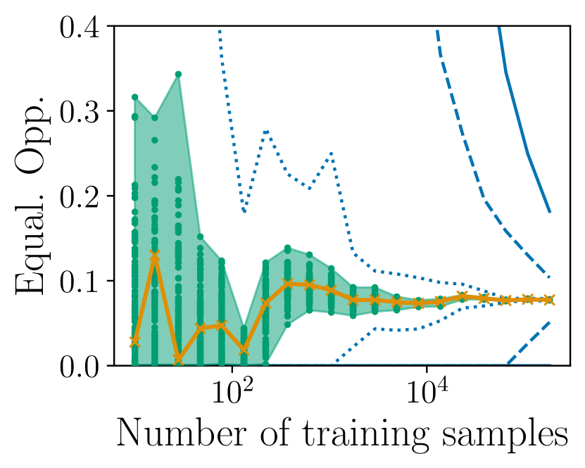
(a) Equal. Opp. (celebA)

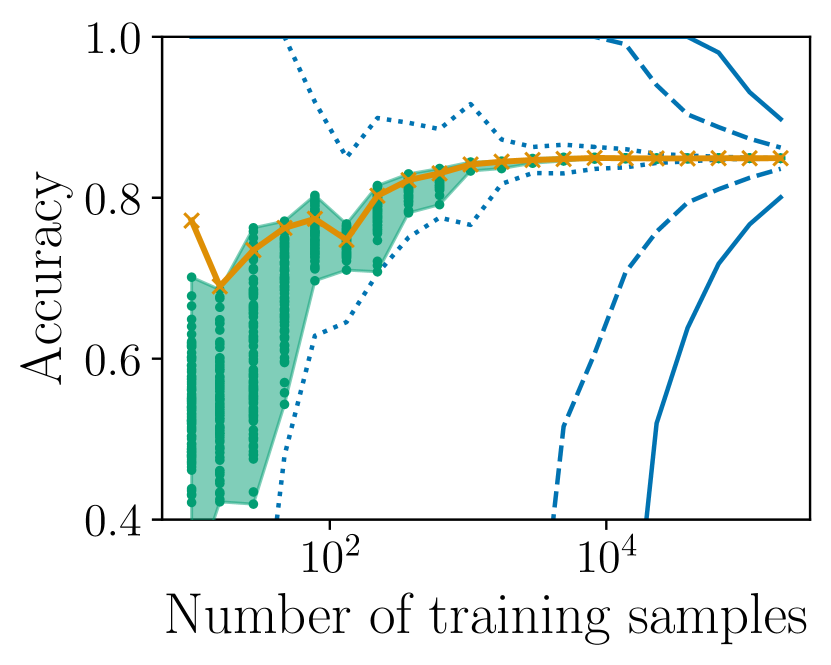
(b) Accuracy (celebA)

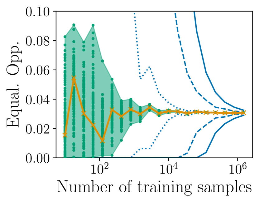
(c) Equal. Opp. (folktables)

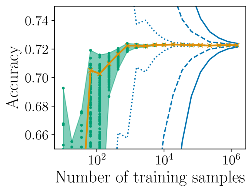
(d) Accuracy (folktables)

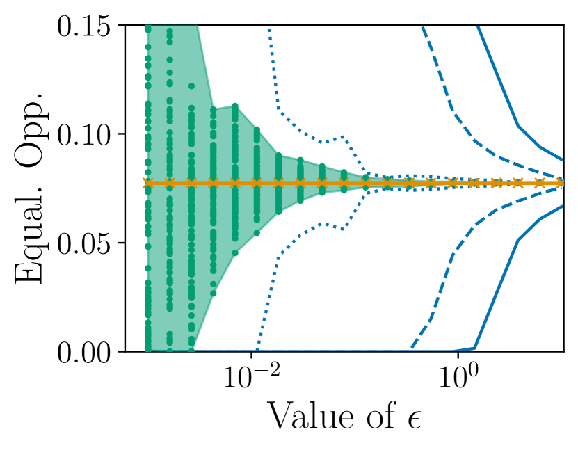
(e) Equal. Opp. (celebA)

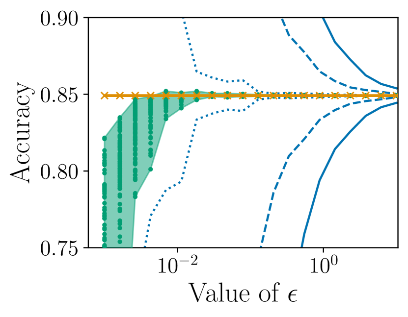
(f) Accuracy (celebA)

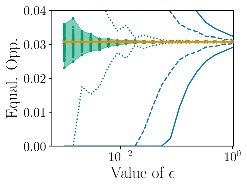
(g) Equal. Opp. (folktables)

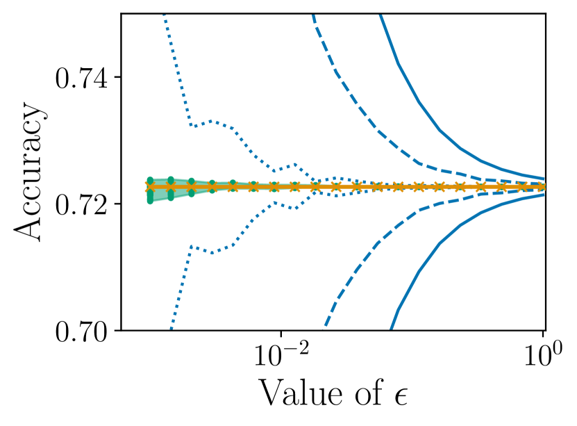
(h) Accuracy (folktables)

Figure 1: Equality of opportunity (Equal. Opp.) and Accuracy levels for optimal non-private model and random private ones as a function of the number of training records $n$ (first line, with $\epsilon=1$ and $\delta=1/n^{2}$) and of the privacy budget $\epsilon$ (second line, using all available training records). For each value of $n$ and $\epsilon$, we sample $100$ private models and take their minimum and maximum fairness/accuracy values to mark the area of attainable values. The solid blue line gives the theoretical guarantees from Theorem 4.4, while the dashed and dotted line give finer bounds when more information is available (see Section 5.3 for details).

5 Numerical Experiments

In this section, we numerically illustrate the upper bounds from Section 4.2. We use the celebA (Liu et al., 2015) and folktables (Ding et al., 2021) datasets, which respectively contain $202,599$ and $1,664,500$ samples, with $39$ and $10$ features (including one sensitive attribute, sex, that is not not used for prediction), and binary labels. For each dataset, we use $90\%$ of the records for training, and the remaining $10\%$ for empirical evaluation of the bounds. We train $\ell_{2}$-regularized logistic regression models, ensuring that the underlying optimization problem is $1$-strongly-convex. This allows learning private models by output perturbation, for which the bound from Theorem 4.4 holds.

In Section 5.1, we show that we obtain non-trivial guarantees on the private model’s fairness and accuracy. Then, we study the influence of the number of training samples and of the privacy budget $\epsilon$ in Section 5.2, and discuss the tightness of our result in Section 5.3.

5.1 Value of the Upper Bounds

In Section 4.1, we compute the value of Theorem 4.4’s bounds. We learn a non-private $\ell_{2}$-regularized logistic regression model, and use it to compute the bounds (averaged over the two groups) for multiple fairness and accuracy measures on two datasets. In all cases, our results give non-trivial guarantees on the difference of fairness: it is bounded by at most $0.105$ for celebA and $0.0026$ for folktables. This means that any $(1,1/n^{2})$-DP model learned by output perturbation will, with high probability, achieve a fairness level within this margin of that of the non-private model.

5.2 Influence of the Number of Training Samples and Privacy Budget

We now verify numerically the rate at which fairness and accuracy levels decrease when increasing the number of training records or privacy budget. In Figure 1, we plot the optimal model’s equality of opportunity and accuracy, as a function of (i) in the first line, the number of samples $n$ used for training, or (ii) in the second line, the privacy budget $\epsilon$ (see Appendix G for results with other fairness measures). For each value of $n$ and $\epsilon$, we plot Theorem 4.4’s theoretical guarantees (solid blue line). With $\epsilon=1$, our bounds give meaningful guarantees for $n\geq 100,000$ records on both celebA and folktables datasets (Figures 0(a), 0(b), 0(c) and 0(d)). When using all records, we obtain meaningful bounds for $\epsilon\geq 1$ for celebA and $\epsilon\geq 0.1$ for folktables (Figures 0(e), 0(f), 0(g) and 0(h)). Additionally, note that we obtain both upper and lower bounds on fairness and accuracy, confirming remarks from Section 3.2.

We also report the fairness and accuracy levels of $100$ private models computed by output perturbation (in green in Figure 1). As predicted by our theory, their fairness and accuracy converges towards the ones of their non-private counterparts as $n$ and $\epsilon$ increase. Interestingly, our bounds seem to follow the same tendency as what we observe empirically (albeit with a larger multiplicative constant), suggesting that they capture the correct dependence in $n$ and $\epsilon$. We further discuss the tightness of our results in next section.

5.3 Tightness of the Bound

We now argue that the two major factors of looseness in our results are (i) the upper bound on $\left\|h^{\mathrm{priv}}-h^{*}\right\|$ and (ii) the looseness of 2.1. While these cannot be improved in general, specific knowledge of $h^{\mathrm{priv}}$ and $h^{*}$ (that is typically not available due to privacy) can lead to tighter bounds. First, when the distance $\left\|h^{\mathrm{priv}}-h^{*}\right\|$ is known, we can use its actual value rather than the upper bounds of Section 4.1 (see dashed blue line in Figure 1). Second, when both $h^{\mathrm{priv}}$ and $h^{*}$ are known, 2.1 can be substantially refined (see details in Section G.3). We evaluate this bound for the private model that is the farthest away from the non-private one (see dotted blue line in Figure 1). The resulting bound appears to be tight up to a small multiplicative constant. These two observations suggest that our bounds cannot be significantly tightened, unless one can obtain such knowledge through either private computation or additional assumptions on the data.

6 Conclusion

In this work, we proved that the fairness (and accuracy) costs induced by privacy in differentially private classification vanishes at a $\widetilde{O}(\nicefrac{{\sqrt{p}}}{{n}})$ rate, where $n$ is the number of training records, and $p$ the number of parameters. This rate follows from a general statement on the regularity of a family of group fairness measures, that we prove to be pointwise Lipschitz with respect to the model. The pointwise Lipschitz constant explicitly depends on the confidence margin of the model, and may be different for each sensitive group. We also show it can be computed from a finite data sample. Importantly, our bounds do not require the knowledge of the optimal (non-private) model: they can thus be used in practical privacy-preserving scenarios. We numerically evaluate our bounds on real datasets, and highlight practical settings where non-trivial guarantees can be obtained.

While we illustrated our results for output perturbation and DP-SGD on strongly-convex problems, we stress that they are more general. Indeed, our Theorem 3.2 holds for any pair of models. Consequently, it would apply to DP-SGD on non-convex problems, provided that we have a bound on the distance between the models obtained with and without privacy. Deriving a tight bound on this distance is a challenging problem, that constitutes an interesting future direction.

Finally, we stress that our results do not provide fairness guarantees per se, but only bound the difference of fairness between models. It is nonetheless a first step towards a more complete understanding of the interplay between privacy, fairness, and accuracy. We believe that our results can guide the design of fairer privacy-preserving machine learning algorithms. A first promising direction in this regard is to combine our bounds with fairness-promoting convex regularizers, as discussed in Remark 4.5. Another direction is the design of methods to privately learn models with large-margin guarantees, as recently considered by Bassily et al. (2022). Our results, which explicitly depend on the confidence margin of the model, suggest that better fairness guarantees could be obtained for these methods.

This appendix provides several examples of group fairness functions compatible with our framework (Appendix A), the proofs of the main theoretical results that were omitted in the main paper for the sake of readability (Appendices B, C, D, E and F), and additional experiments (Appendix G).

Appendix A Fairness functions

In this section we recall several well known fairness functions and show that they can be written in the form of Equation 1.

Example 1 (Equalized Odds (Hardt et al., 2016)).

A model $h$ is fair for Equalized Odds when the probability of predicting the correct label is independent of the sensitive attribute, that is, $\forall(y,r)\in\mathcal{Y}\times\mathcal{S}$

$$F_{(y,r)}(h,D)=\operatorname*{\mathbb{P}}\left(H(X)=Y\;\middle|\;Y=y,S=r\right)-\operatorname*{\mathbb{P}}\left(H(X)=Y\;\middle|\;Y=y\right).$$

We can then write $F_{(y,r)}(h,D)$ in the form of Equation (1) as

$$F_{(y,r)}(h,D)=C_{(y,r)}^{0}+\sum_{(y^{\prime},r^{\prime})\in\mathcal{Y}\times\mathcal{S}}C_{(y,r)}^{(y^{\prime},r^{\prime})}\operatorname*{\mathbb{P}}\left(H(x)=Y|Y=y^{\prime},S=r^{\prime}\right)$$ (4)

with

$$C_{(y,r)}^{0}={} 0$$

$$C_{(y,r)}^{(y,r)}={} 1-\operatorname*{\mathbb{P}}\left(S=r\;\middle|\;Y=y\right)$$

$$\text{ $\forall r^{\prime}\neq r$, }C_{(y,r)}^{(y,r^{\prime})}={} -\operatorname*{\mathbb{P}}\left(S=r^{\prime}\;\middle|\;Y=y\right)$$

$$\text{ $\forall y^{\prime}\neq y$, $\forall r^{\prime}\in\mathcal{S}$, }C_{(y,r)}^{(y^{\prime},r^{\prime})}={} 0$$

Proof.

We have that

$$F_{(y,r)}(h,D)={} \operatorname*{\mathbb{P}}\left(H(X)=Y\;\middle|\;Y=y,S=r\right)-\operatorname*{\mathbb{P}}\left(H(X)=Y\;\middle|\;Y=y\right)$$

$$={} \operatorname*{\mathbb{P}}\left(H(X)=Y\;\middle|\;Y=y,S=r\right)-\sum_{r^{\prime}\in\mathcal{S}}\operatorname*{\mathbb{P}}\left(H(X)=Y\;\middle|\;Y=y,S=r^{\prime}\right)\operatorname*{\mathbb{P}}\left(S=r^{\prime}\;\middle|\;Y=y\right)$$

which gives the result. ∎

Example 2 (Equality of Opportunity (Hardt et al., 2016)).

A model $h$ is fair for Equality of Opportunity when the probability of predicting the correct label is independent of the sensitive attribute for the set of desirable outcomes $\mathcal{Y}^{\prime}\subset\mathcal{Y}$, that is $\forall(y,r)\in\mathcal{Y}\times\mathcal{S}$

$$F_{(y,r)}(h,D)=\left\{\begin{array}[]{ll}\operatorname*{\mathbb{P}}\left(H(X)=Y\;\middle|\;Y=y,S=r\right)-\operatorname*{\mathbb{P}}\left(H(X)=Y\;\middle|\;Y=y\right)&\text{if $y\in\mathcal{Y}^{\prime}$,}\\ 0&\text{otherwise.}\end{array}\right.$$

We can then write $F_{(y,r)}(h,D)$ in the form of Equation (1) as

$$F_{(y,r)}(h,D)=C_{(y,r)}^{0}+\sum_{(y^{\prime},r^{\prime})\in\mathcal{Y}\times\mathcal{S}}C_{(y,r)}^{(y^{\prime},r^{\prime})}\operatorname*{\mathbb{P}}\left(H(X)=Y|Y=y^{\prime},S=r^{\prime}\right)$$ (5)

with, if $y\in\mathcal{Y}^{\prime}$,

$$C_{(y,r)}^{0}={} 0$$

$$C_{(y,r)}^{(y,r)}={} 1-\operatorname*{\mathbb{P}}\left(S=r\;\middle|\;Y=y\right)$$

$$\text{$\forall r^{\prime}\neq r$, }C_{(y,r)}^{(y,r^{\prime})}={} -\operatorname*{\mathbb{P}}\left(S=r^{\prime}\;\middle|\;Y=y\right)$$

$$\text{$\forall y^{\prime}\neq y$, $\forall r^{\prime}\in\mathcal{S}$, }C_{(y,r)}^{(y^{\prime},r^{\prime})}={} 0$$

and, if $y\in\mathcal{Y}\setminus\mathcal{Y}^{\prime}$,

$$\text{$\forall y^{\prime}\in\mathcal{Y}$, $\forall r^{\prime}\in\mathcal{S}$, }C_{(y,r)}^{(y^{\prime},r^{\prime})}=0.$$

Proof.

We consider the two cases. On the one hand, when $y\in\mathcal{Y}\setminus\mathcal{Y}^{\prime}$, then we have that

$$F_{(y,r)}(h,D)={}0$$

which gives the first part of the result. On the other hand, when $y\in\mathcal{Y}^{\prime}$, then we have that

$$F_{(y,r)}(h,D)={} \operatorname*{\mathbb{P}}\left(H(X)=Y\;\middle|\;Y=y,S=r\right)-\operatorname*{\mathbb{P}}\left(H(X)=Y\;\middle|\;Y=y\right)$$

$$={} \operatorname*{\mathbb{P}}\left(H(X)=Y\;\middle|\;Y=y,S=r\right)-\sum_{r^{\prime}\in\mathcal{S}}\operatorname*{\mathbb{P}}\left(H(X)=Y\;\middle|\;Y=y,S=r^{\prime}\right)\operatorname*{\mathbb{P}}\left(S=r^{\prime}\;\middle|\;Y=y\right)$$

which gives the second part of the result. ∎

Example 3 (Accuracy Parity (Zafar et al., 2017)).

A model $h$ is fair for Accuracy Parity when the probability of being correct is independent of the sensitive attribute, that is, $\forall(r)\in\mathcal{S}$

$$F_{(r)}(h,D)=\operatorname*{\mathbb{P}}\left(H(X)=Y\;\middle|\;S=r\right)-\operatorname*{\mathbb{P}}\left(H(X)=Y\right).$$

We can then write $F_{(r)}(h,D)$ in the form of Equation (1) as

$$F_{(r)}(h,D)=C_{(r)}^{0}+\sum_{(r^{\prime})\in\mathcal{S}}C_{(r)}^{(r^{\prime})}\operatorname*{\mathbb{P}}\left(H(X)=Y|S=r^{\prime}\right)$$ (6)

with

$$C_{(r)}^{0}={} 0$$

$$C_{(r)}^{(r)}={} 1-\operatorname*{\mathbb{P}}\left(S=r\right)$$

$$\text{ $\forall r^{\prime}\neq r$, }C_{(r)}^{(r^{\prime})}={} -\operatorname*{\mathbb{P}}\left(S=r^{\prime}\right)$$

Proof.

We have that

$$F_{(r)}(h,D)={} \operatorname*{\mathbb{P}}\left(H(X)=Y\;\middle|\;S=r\right)-\operatorname*{\mathbb{P}}\left(H(X)=Y\right)$$

$$={} \operatorname*{\mathbb{P}}\left(H(X)=Y\;\middle|\;S=r\right)-\sum_{r^{\prime}\in\mathcal{S}}\operatorname*{\mathbb{P}}\left(H(X)=Y\;\middle|\;S=r^{\prime}\right)\operatorname*{\mathbb{P}}\left(S=r^{\prime}\right)$$

which gives the result. ∎

Example 4 (Demographic Parity (Binary Labels) (Calders et al., 2009)).

A model $h$ is fair for Demographic Parity with binary labels when the probability of predicting a label is independent of the sensitive attribute, that is, $\forall(y,r)\in\mathcal{Y}\times\mathcal{S}$

$$F_{(y,r)}(h,D)=\operatorname*{\mathbb{P}}\left(H(X)=y\;\middle|\;S=r\right)-\operatorname*{\mathbb{P}}\left(H(X)=y\right).$$

Assuming that given a label $y$, the second binary label is denoted $\bar{y}$, we can then write $F_{(y,r)}(h,D)$ in the form of Equation (1) as

$$F_{(y,r)}(h,D)=C_{(y,r)}^{0}+\sum_{(y^{\prime},r^{\prime})\in\mathcal{Y}\times\mathcal{S}}C_{(y,r)}^{(y^{\prime},r^{\prime})}\operatorname*{\mathbb{P}}\left(H(X)=Y|Y=y^{\prime},S=r^{\prime}\right)$$ (7)

with

$$C_{(y,r)}^{0}={} \operatorname*{\mathbb{P}}\left(Y=y\right)-\operatorname*{\mathbb{P}}\left(Y=y\;\middle|\;S=r\right)$$

$$C_{(y,r)}^{(y,r)}={} \operatorname*{\mathbb{P}}\left(Y=y\;\middle|\;S=r\right)-\operatorname*{\mathbb{P}}\left(Y=y,S=r\right)$$

$$C_{(y,r)}^{(\bar{y},r)}={} \operatorname*{\mathbb{P}}\left(Y=\bar{y},S=r\right)-\operatorname*{\mathbb{P}}\left(Y=\bar{y}\;\middle|\;S=r\right)$$

$$\text{ $\forall r^{\prime}\neq r$, }C_{(y,r)}^{(y,r^{\prime})}={} -\operatorname*{\mathbb{P}}\left(Y=y,S=r^{\prime}\right)$$

$$\text{ $\forall r^{\prime}\neq r$, }C_{(y,r)}^{(\bar{y},r^{\prime})}={} \operatorname*{\mathbb{P}}\left(Y=\bar{y},S=r^{\prime}\right)$$

Proof.

We have that

$$F_{(y,r)}(h,D)={} \operatorname*{\mathbb{P}}\left(H(X)=y\;\middle|\;S=r\right)-\operatorname*{\mathbb{P}}\left(H(X)=y\right)$$

$$={} \operatorname*{\mathbb{P}}\left(H(X)=y\;\middle|\;Y=y,S=r\right)\operatorname*{\mathbb{P}}\left(Y=y\;\middle|\;S=r\right)+\operatorname*{\mathbb{P}}\left(H(X)=y\;\middle|\;Y\neq y,S=r\right)\operatorname*{\mathbb{P}}\left(Y\neq y\;\middle|\;S=r\right)$$

$$-\sum_{r^{\prime}\in\mathcal{S}}\big{(}\operatorname*{\mathbb{P}}\left(H(X)=y\;\middle|\;Y=y,S=r^{\prime}\right)\operatorname*{\mathbb{P}}\left(Y=y,S=r^{\prime}\right)$$

$$\qquad\qquad+\operatorname*{\mathbb{P}}\left(H(X)=y\;\middle|\;Y\neq y,S=r^{\prime}\right)\operatorname*{\mathbb{P}}\left(Y\neq y,S=r^{\prime}\right)\big{)}$$

$$={} \operatorname*{\mathbb{P}}\left(H(X)=y\;\middle|\;Y=y,S=r\right)\operatorname*{\mathbb{P}}\left(Y=y\;\middle|\;S=r\right)$$

$$\quad+1-\operatorname*{\mathbb{P}}\left(H(X)\neq y\;\middle|\;Y\neq y,S=r\right)\operatorname*{\mathbb{P}}\left(Y\neq y\;\middle|\;S=r\right)$$

$$-\sum_{r^{\prime}\in\mathcal{S}}\big{(}\operatorname*{\mathbb{P}}\left(H(X)=y\;\middle|\;Y=y,S=r^{\prime}\right)\operatorname*{\mathbb{P}}\left(Y=y,S=r^{\prime}\right)$$

$$\qquad\qquad+1-\operatorname*{\mathbb{P}}\left(H(X)\neq y\;\middle|\;Y\neq y,S=r^{\prime}\right)\operatorname*{\mathbb{P}}\left(Y\neq y,S=r^{\prime}\right)\big{)}.$$

Here, we only consider binary labels, $y$ and $\bar{y}$. Hence, $H(X)\neq y\Leftrightarrow H(X)=\bar{y}$ and $Y\neq y\Leftrightarrow Y=\bar{y}$. Thus, we obtain

$$F_{(y,r)} (h,D)$$

$$={} \operatorname*{\mathbb{P}}\left(H(X)=y\;\middle|\;Y=y,S=r\right)\operatorname*{\mathbb{P}}\left(Y=y\;\middle|\;S=r\right)+\left(1-\operatorname*{\mathbb{P}}\left(H(X)=\bar{y}\;\middle|\;Y=\bar{y},S=r\right)\right)\operatorname*{\mathbb{P}}\left(Y=\bar{y}\;\middle|\;S=r\right)$$

$$-\sum_{r^{\prime}\in\mathcal{S}}\big{(}\operatorname*{\mathbb{P}}\left(H(X)=y\;\middle|\;Y=y,S=r^{\prime}\right)\operatorname*{\mathbb{P}}\left(Y=y,S=r^{\prime}\right)$$

$$\qquad\qquad+\left(1-\operatorname*{\mathbb{P}}\left(H(X)=\bar{y}\;\middle|\;Y=\bar{y},S=r^{\prime}\right)\right)\operatorname*{\mathbb{P}}\left(Y=\bar{y},S=r^{\prime}\right)\big{)}$$

$$={} \operatorname*{\mathbb{P}}\left(H(X)=y\;\middle|\;Y=y,S=r\right)\left[\operatorname*{\mathbb{P}}\left(Y=y\;\middle|\;S=r\right)-\operatorname*{\mathbb{P}}\left(Y=y,S=r\right)\right]$$

$$+\operatorname*{\mathbb{P}}\left(H(X)=\bar{y}\;\middle|\;Y=\bar{y},S=r\right)\left[\operatorname*{\mathbb{P}}\left(Y=\bar{y},S=r\right)-\operatorname*{\mathbb{P}}\left(Y=\bar{y}\;\middle|\;S=r\right)\right]$$

$$+\sum_{r^{\prime}\in\mathcal{S},r^{\prime}\neq r}\operatorname*{\mathbb{P}}\left(H(X)=y\;\middle|\;Y=y,S=r^{\prime}\right)\left(-\operatorname*{\mathbb{P}}\left(Y=y,S=r^{\prime}\right)\right)$$

$$+\sum_{r^{\prime}\in\mathcal{S},r^{\prime}\neq r}\operatorname*{\mathbb{P}}\left(H(X)=\bar{y}\;\middle|\;Y=\bar{y},S=r^{\prime}\right)\operatorname*{\mathbb{P}}\left(Y=\bar{y},S=r^{\prime}\right)$$

$$+\operatorname*{\mathbb{P}}\left(Y=\bar{y}\;\middle|\;S=r\right)-\operatorname*{\mathbb{P}}\left(Y=\bar{y}\right)$$

$$={} \operatorname*{\mathbb{P}}\left(H(X)=Y\;\middle|\;Y=y,S=r\right)\left[\operatorname*{\mathbb{P}}\left(Y=y\;\middle|\;S=r\right)-\operatorname*{\mathbb{P}}\left(Y=y,S=r\right)\right]$$

$$+\operatorname*{\mathbb{P}}\left(H(X)=Y\;\middle|\;Y=\bar{y},S=r\right)\left[\operatorname*{\mathbb{P}}\left(Y=\bar{y},S=r\right)-\operatorname*{\mathbb{P}}\left(Y=\bar{y}\;\middle|\;S=r\right)\right]$$

$$+\sum_{r^{\prime}\in\mathcal{S},r^{\prime}\neq r}\operatorname*{\mathbb{P}}\left(H(X)=Y\;\middle|\;Y=y,S=r^{\prime}\right)\left(-\operatorname*{\mathbb{P}}\left(Y=y,S=r^{\prime}\right)\right)$$

$$+\sum_{r^{\prime}\in\mathcal{S},r^{\prime}\neq r}\operatorname*{\mathbb{P}}\left(H(X)=Y\;\middle|\;Y=\bar{y},S=r^{\prime}\right)\operatorname*{\mathbb{P}}\left(Y=\bar{y},S=r^{\prime}\right)$$

$$+\operatorname*{\mathbb{P}}\left(Y=y\right)-\operatorname*{\mathbb{P}}\left(Y=y\;\middle|\;S=r\right)$$

which gives the result. ∎

Appendix B Proof of Theorem 3.1

Theorem (Pointwise Lipschitzness of Conditional Negative Predictions).

Let $\mathcal{H}$ be a set of real vector-valued functions with $L_{X,Y}$ the Lipschitz constants defined in 2.1. Let $h,h^{\prime}\in\mathcal{H}$ be two models, $(X,Y,S)$ be a triple of random variables having distribution $\mathcal{D}$, and $E$ be an arbitrary event. Assume that $\operatorname*{\mathbb{E}}\left(\frac{L_{X,Y}}{\left|\rho(h,X,Y)\right|}\;\middle|\;E\right)<+\infty$, then

$$\left|\operatorname*{\mathbb{P}}(H(X)=Y\;\middle|\;E)-\operatorname*{\mathbb{P}}(H^{\prime}(X)=Y\;\middle|\;E)\right|\leq\operatorname*{\mathbb{E}}\left(\frac{L_{X,Y}}{\left|\rho(h,X,Y)\right|}\;\middle|\;E\right)\left\|h-h^{\prime}\right\|_{\mathcal{H}}\enspace.$$

Proof.

The proof of this theorem is in two steps. First, we use the Lipschitz continuity property associated with $\mathcal{H}$, the triangle inequality, and the union bound to show that $\left|\operatorname*{\mathbb{P}}\left(H(X)=Y\;\middle|\;E\right)-\operatorname*{\mathbb{P}}\left(H^{\prime}(X)=Y\;\middle|\;E\right)\right|\leq{}\operatorname*{\mathbb{P}}\left(\frac{L_{X,Y}}{\left|\rho(h,X,Y)\right|}\leq\left\|h-h^{\prime}\right\|_{\mathcal{H}}\;\middle|\;E\right)$. Then, applying Markov’s inequality gives the desired result.

Bounding $\left|\operatorname*{\mathbb{P}}\left(H(X)=Y\;\middle|\;E\right)-\operatorname*{\mathbb{P}}\left(H^{\prime}(X)=Y\;\middle|\;E\right)\right|$.

We have that

$$\operatorname*{\mathbb{P}}\left(H(X)=Y\;\middle|\;E\right)- \operatorname*{\mathbb{P}}\left(H^{\prime}(X)=Y\;\middle|\;E\right)$$

$$\leq{} \operatorname*{\mathbb{P}}\left(\rho(h,X,Y)\geq 0\;\middle|\;E\right)-\operatorname*{\mathbb{P}}\left(\rho(h^{\prime},X,Y)>0\;\middle|\;E\right)$$

$$={} \operatorname*{\mathbb{P}}\left(\rho(h^{\prime},X,Y)\leq 0\;\middle|\;E\right)-\operatorname*{\mathbb{P}}\left(\rho(h,X,Y)<0\;\middle|\;E\right)$$

$$={} \operatorname*{\mathbb{P}}\left(\rho(h^{\prime},X,Y)-\rho(h,X,Y)+\rho(h,X,Y)\leq 0\;\middle|\;E\right)-\operatorname*{\mathbb{P}}\left(\rho(h,X,Y)<0\;\middle|\;E\right)$$

$$={} \operatorname*{\mathbb{P}}\left(\rho(h,X,Y)\leq\rho(h,X,Y)-\rho(h^{\prime},X,Y)\;\middle|\;E\right)-\operatorname*{\mathbb{P}}\left(\rho(h,X,Y)<0\;\middle|\;E\right)$$

$$\leq{} \operatorname*{\mathbb{P}}\left(\rho(h,X,Y)\leq\left|\rho(h,X,Y)-\rho(h^{\prime},X,Y)\right|\;\middle|\;E\right)-\operatorname*{\mathbb{P}}\left(\rho(h,X,Y)<0\;\middle|\;E\right)$$

$${\color[rgb]{.5,.5,.5}\downarrow{}\;{\small\text{\lx@cref{creftypecap~refnum}{assum:lipschitz-constant-fct-val}.}}}$$

$$\leq{} \operatorname*{\mathbb{P}}\left(\rho(h,X,Y)\leq L_{X,Y}\left\|h-h^{\prime}\right\|_{\mathcal{H}}\;\middle|\;E\right)-\operatorname*{\mathbb{P}}\left(\rho(h,X,Y)<0\;\middle|\;E\right)$$

$$={} \operatorname*{\mathbb{P}}\left(\rho(h,X,Y)<0\bigcup 0\leq\rho(h,X,Y)\leq L_{X,Y}\left\|h-h^{\prime}\right\|_{\mathcal{H}}\;\middle|\;E\right)-\operatorname*{\mathbb{P}}\left(\rho(h,X,Y)<0\;\middle|\;E\right)$$

$${\color[rgb]{.5,.5,.5}\downarrow{}\;{\small\text{Union bound on disjoint events.}}}$$

$$={} \operatorname*{\mathbb{P}}\left(0\leq\rho(h,X,Y)\leq L_{X,Y}\left\|h-h^{\prime}\right\|_{\mathcal{H}}\;\middle|\;E\right)$$

$$\leq{} \operatorname*{\mathbb{P}}\left(\left|\rho(h,X,Y)\right|\leq L_{X,Y}\left\|h-h^{\prime}\right\|_{\mathcal{H}}\;\middle|\;E\right)$$

$$={} \operatorname*{\mathbb{P}}\left(\frac{\left|\rho(h,X,Y)\right|}{L_{X,Y}}\leq\left\|h-h^{\prime}\right\|_{\mathcal{H}}\;\middle|\;E\right)$$

Similarly, we have that

$$\operatorname*{\mathbb{P}}\left(H^{\prime}(X)=Y\;\middle|\;E\right)- \operatorname*{\mathbb{P}}\left(H(X)=Y\;\middle|\;E\right)$$

$$\leq{} \operatorname*{\mathbb{P}}\left(\rho(h^{\prime},X,Y)\geq 0\;\middle|\;E\right)-\operatorname*{\mathbb{P}}\left(\rho(h,X,Y)>0\;\middle|\;E\right)$$

$$={} \operatorname*{\mathbb{P}}\left(\rho(h^{\prime},X,Y)+\rho(h,X,Y)-\rho(h,X,Y)\geq 0\;\middle|\;E\right)-\operatorname*{\mathbb{P}}\left(\rho(h,X,Y)>0\;\middle|\;E\right)$$

$$={} \operatorname*{\mathbb{P}}\left(\rho(h,X,Y)\geq-\left(\rho(h^{\prime},X,Y)-\rho(h,X,Y)\right)\;\middle|\;E\right)-\operatorname*{\mathbb{P}}\left(\rho(h,X,Y)>0\;\middle|\;E\right)$$

$$\leq{} \operatorname*{\mathbb{P}}\left(\rho(h,X,Y)\geq-\left|\rho(h^{\prime},X,Y)-\rho(h,X,Y)\right|\;\middle|\;E\right)-\operatorname*{\mathbb{P}}\left(\rho(h,X,Y)>0\;\middle|\;E\right)$$

$${\color[rgb]{.5,.5,.5}\downarrow{}\;{\small\text{\lx@cref{creftypecap~refnum}{assum:lipschitz-constant-fct-val}}}}$$

$$\leq{} \operatorname*{\mathbb{P}}\left(\rho(h,X,Y)\geq-L_{X,Y}\left\|h-h^{\prime}\right\|_{\mathcal{H}}\;\middle|\;E\right)-\operatorname*{\mathbb{P}}\left(\rho(h,X,Y)>0\;\middle|\;E\right)$$

$$={} \operatorname*{\mathbb{P}}\left(\rho(h,X,Y)>0\bigcup 0\geq\rho(h,X,Y)\geq-L_{X,Y}\left\|h-h^{\prime}\right\|_{\mathcal{H}}\;\middle|\;E\right)-\operatorname*{\mathbb{P}}\left(\rho(h,X,Y)>0\;\middle|\;E\right)$$

$${\color[rgb]{.5,.5,.5}\downarrow{}\;{\small\text{Union bound on disjoint events.}}}$$

$$={} \operatorname*{\mathbb{P}}\left(0\geq\rho(h,X,Y)\geq-L_{X,Y}\left\|h-h^{\prime}\right\|_{\mathcal{H}}\;\middle|\;E\right)$$

$$\leq{} \operatorname*{\mathbb{P}}\left(-\left|\rho(h,X,Y)\right|\geq-L_{X,Y}\left\|h-h^{\prime}\right\|_{\mathcal{H}}\;\middle|\;E\right)$$

$$={} \operatorname*{\mathbb{P}}\left(\frac{\left|\rho(h,X,Y)\right|}{L_{X,Y}}\leq\left\|h-h^{\prime}\right\|_{\mathcal{H}}\;\middle|\;E\right)$$

It implies that

$$\left|\operatorname*{\mathbb{P}}\left(H(X)=Y\;\middle|\;E\right)-\operatorname*{\mathbb{P}}\left(H^{\prime}(X)=Y\;\middle|\;E\right)\right|\leq{}\operatorname*{\mathbb{P}}\left(\frac{\left|\rho(h,X,Y)\right|}{L_{X,Y}}\leq\left\|h-h^{\prime}\right\|_{\mathcal{H}}\;\middle|\;E\right)$$

Bounding $\operatorname*{\mathbb{P}}\left(\frac{\left|\rho(h,X,Y)\right|}{L_{X,Y}}\leq\left\|h-h^{\prime}\right\|_{\mathcal{H}}\;\middle|\;E\right)$.

We use the Markov’s Inequality and we assume that $\operatorname*{\mathbb{E}}\left(\frac{L_{X,Y}}{\left|\rho(h,X,Y)\right|}\;\middle|\;E\right)<+\infty$. Hence, we have that

$$\operatorname*{\mathbb{P}}\left(\frac{\left|\rho(h,X,Y)\right|}{L_{X,Y}}\leq\left\|h-h^{\prime}\right\|_{\mathcal{H}}\;\middle|\;E\right)={} \operatorname*{\mathbb{P}}\left(\frac{L_{X,Y}}{\left|\rho(h,X,Y)\right|}\geq\frac{1}{\left\|h-h^{\prime}\right\|_{\mathcal{H}}}\;\middle|\;E\right)$$

$${\color[rgb]{.5,.5,.5}\downarrow{}\;{\small\text{Markov's inequality.}}}$$

$$\leq{} \operatorname*{\mathbb{E}}\left(\frac{L_{X,Y}}{\left|\rho(h,X,Y)\right|}\;\middle|\;E\right)\left\|h-h^{\prime}\right\|_{\mathcal{H}}$$

It concludes the proof. ∎

Remark B.1.

In the last step of the proof of Theorem 3.1, we can also use the Chernoff bound:

$$\operatorname*{\mathbb{P}}\left(\frac{\left|\rho(h,X,Y)\right|}{L_{X,Y}}\leq\left\|h-h^{\prime}\right\|_{\mathcal{H}}\;\middle|\;E\right)={} \operatorname*{\mathbb{P}}\left(\exp\left(-t\frac{\left|\rho(h,X,Y)\right|}{L_{X,Y}}\right)\geq\exp\left(-t\left\|h-h^{\prime}\right\|_{\mathcal{H}}\right)\;\middle|\;E\right)$$

$$\leq{} \operatorname*{\mathbb{E}}\left(\exp\left(-t\frac{\left|\rho(h,X,Y)\right|}{L_{X,Y}}\right)\;\middle|\;E\right)\exp\left(t\left\|h-h^{\prime}\right\|_{\mathcal{H}}\right)\enspace.$$

A correct choice of $t$ would lead to potentially tighter bounds than the Markov’s inequality at the expense of readability.

Remark B.2.

Before using Markov’s inequality or Chernoff bound in Theorem 3.1, we can modify the probability as

$$\operatorname*{\mathbb{P}}\left(\frac{\left|\rho(h,X,Y)\right|}{L_{X,Y}}\leq\left\|h-h^{\prime}\right\|_{\mathcal{H}}\;\middle|\;E\right)={} \operatorname*{\mathbb{P}}\left(\left[\frac{\left|\rho(h,X,Y)\right|}{L_{X,Y}}\right]^{\left\|h-h^{\prime}\right\|_{\mathcal{H}}}\leq\left\|h-h^{\prime}\right\|_{\mathcal{H}}\;\middle|\;E\right)\enspace,$$

where

$$\left[\frac{\left|\rho(h,X,Y)\right|}{L_{X,Y}}\right]^{\left\|h-h^{\prime}\right\|_{\mathcal{H}}} =\begin{cases}\frac{\left|\rho(h,X,Y)\right|}{L_{X,Y}}&\text{if~{}~{}}\left|\rho(h,X,Y)\right|\leq L_{X,Y}\left\|h-h^{\prime}\right\|_{\mathcal{H}}\enspace,\\ +\infty&\text{otherwise}\enspace.\end{cases}$$

This essentially means that, whenever the model’s margin on a data record is large enough, its precise value is no more meaningful, as its prediction will not change whatsoever. The remaining of Theorem 3.1’s proof is unchanged, except with $\left[\frac{\left|\rho(h,X,Y)\right|}{L_{X,Y}}\right]^{\left\|h-h^{\prime}\right\|_{\mathcal{H}}}$ instead of $\frac{\left|\rho(h,X,Y)\right|}{L_{X,Y}}$.

Note that this can lead to much tighter bounds. Notably, when distance $\left\|h-h^{\prime}\right\|_{\mathcal{H}}$ between $h$ and $h^{\prime}$ is small enough, the difference of fairness may even become zero.

Appendix C Proof of Theorem 3.2

Theorem (Pointwise Lipschitzness of Fairness).

Let $h,h^{\prime}\in\mathcal{H}$, $L_{X,Y}$ be defined as in 2.1, and $(X,S,Y)\sim\mathcal{D}$. For any fairness notion of the form of Equation (1), we have:

$$\forall k\in[K],\left|F_{k}(h,D)-F_{k}(h^{\prime},D)\right|\leq\chi_{k}(h,D)\left\|h-h^{\prime}\right\|_{\mathcal{H}}\enspace,$$

with $\chi_{k}(h,D)=\sum_{k^{\prime}=1}^{K}\left|C_{k}^{k^{\prime}}\right|\operatorname*{\mathbb{E}}\left(\frac{1}{\left|h(X)\right|}\;\middle|\;D_{k^{\prime}}\right)$. Similarly, for the aggregate measure of fairness defined in Equation (2), we have:

$$\left|\text{Fair}(h,D)-\text{Fair}(h^{\prime},D)\right|\leq\frac{1}{K}\sum_{k=1}^{K}\chi_{k}(h,D)\left\|h-h^{\prime}\right\|_{\mathcal{H}}\enspace.$$

Proof.

The first part follows from the following derivation. For all $k$,

$$\left|F_{k}(h,D)-F_{k}(h^{\prime},D)\right|={} \left|C_{k}^{0}+\sum_{k^{\prime}=1}^{K}C_{k}^{k^{\prime}}\operatorname*{\mathbb{P}}\left(H(X)=Y|D_{k^{\prime}}\right)-C_{k}^{0}-\sum_{k^{\prime}=1}^{K}C_{k}^{k^{\prime}}\operatorname*{\mathbb{P}}\left(H^{\prime}(X)=Y|D_{k^{\prime}}\right)\right|$$

$$={} \left|\sum_{k^{\prime}=1}^{K}C_{k}^{k^{\prime}}\Big{(}\operatorname*{\mathbb{P}}\left(H(X)=Y|D_{k^{\prime}}\right)-\operatorname*{\mathbb{P}}\left(H^{\prime}(X)=Y|D_{k^{\prime}}\right)\Big{)}\right|$$

$${\color[rgb]{.5,.5,.5}\downarrow{}\;{\small\text{Triangle inequality.}}}$$

$$\leq{} \sum_{k^{\prime}=1}^{K}\left|C_{k}^{k^{\prime}}\right|\left|\operatorname*{\mathbb{P}}\left(H(X)=Y|D_{k^{\prime}}\right)-\operatorname*{\mathbb{P}}\left(H^{\prime}(X)=Y|D_{k^{\prime}}\right)\right|$$

$${\color[rgb]{.5,.5,.5}\downarrow{}\;{\small\text{Theorem~{}\ref{thm:bound-on-diff-proba}.}}}$$

$$\leq{} \sum_{k^{\prime}=1}^{K}\left|C_{k}^{k^{\prime}}\right|\operatorname*{\mathbb{E}}\left(\frac{L_{X,Y}}{\left|\rho(h,X,Y)\right|}\;\middle|\;D_{k^{\prime}}\right)\left\|h-h^{\prime}\right\|_{\mathcal{H}}\enspace.$$

The second part is obtained thanks to the triangle inequality:

$$\left|\text{Fair}(h,D)-\text{Fair}(h^{\prime},D)\right|={} \left|\frac{1}{K}\sum_{k=1}^{K}\left|F_{k}(h,D)\right|-\frac{1}{K}\sum_{k=1}^{K}\left|F_{k}(h^{\prime},D)\right|\right|$$

$${\color[rgb]{.5,.5,.5}\downarrow{}\;{\small\text{Triangle inequality.}}}$$

$$\leq{} \frac{1}{K}\sum_{k=1}^{K}\left|\left|F_{k}(h,D)\right|-\left|F_{k}(h^{\prime},D)\right|\right|$$

$${\color[rgb]{.5,.5,.5}\downarrow{}\;{\small\text{Reverse triangle inequality.}}}$$

$$\leq{} \frac{1}{K}\sum_{k=1}^{K}\left|F_{k}(h,D)-F_{k}(h^{\prime},D)\right|\enspace,$$

which gives the claim when combined with the first part of the theorem. ∎

Appendix D Proof of Lemma 3.4

Lemma (Finite Sample analysis).

Let $D$ be a finite sample of $n\geq\frac{8\log\left(\frac{2K+1}{\delta}\right)}{\min_{k^{\prime}}p_{k^{\prime}}}$ examples drawn i.i.d. from $\mathcal{D}$, where $p_{k^{\prime}}$ is the true proportion of examples from group $k^{\prime}$. Assume that $\operatorname*{\mathbb{P}}_{D\sim\mathcal{D}^{n}}\big{(}\sum_{k^{\prime}=0}^{K}\big{|}C_{k}^{k^{\prime}}-\widehat{C}_{k}^{k^{\prime}}\big{|}>\alpha_{C}\big{)}\leq B_{3}\exp\left(-B_{4}\alpha_{C}^{2}n\right)$. Let $\mathcal{H}$ be an hypothesis space and $d_{\mathcal{H}}$ be the Natarajan dimension of $\mathcal{H}$.

• Assuming that $h$ and $h^{\prime}$ are independent of $D$. With probability $1-\delta$ over the choice of $D$,

  $$\left|F_{k}(h,D)-\widehat{F}_{k}(h^{\prime},D)\right|\leq{}\widehat{\chi}_{k}(h,D)\left\|h-h^{\prime}\right\|_{\mathcal{H}}+\widetilde{O}\left(\sum_{k^{\prime}=1}^{K}\left|\widehat{C}_{k}^{k^{\prime}}\right|\sqrt{\frac{\log\left(\nicefrac{{K}}{{\delta}}\right)}{np_{k^{\prime}}}}\right)$$

• Assuming that $h$ and $h^{\prime}$ are dependent of $D$. With probability $1-\delta$ over the choice of $D$, $\forall h,h^{\prime}\in\mathcal{H}$,

  $$\left|F_{k}(h,D)-\widehat{F}_{k}(h^{\prime},D)\right|\leq\widehat{\chi}_{k}(h,D)\left\|h-h^{\prime}\right\|_{\mathcal{H}}+\widetilde{O}\left(\sum_{k^{\prime}=1}^{K}\left|\widehat{C}_{k}^{k^{\prime}}\right|\sqrt{\frac{d_{\mathcal{H}}+\log\left(\nicefrac{{K}}{{\delta}}\right)}{np_{k^{\prime}}}}\right)$$

Proof.

First of all, notice that we have

$$\left|F_{k}(h,D)-\widehat{F}_{k}(h^{\prime},D)\right|={} \left|F_{k}(h,D)-\widehat{F}_{k}(h,D)+\widehat{F}_{k}(h,D)-\widehat{F}_{k}(h^{\prime},D)\right|$$

$$\leq{} \left|F_{k}(h,D)-\widehat{F}_{k}(h,D)\right|+\left|\widehat{F}_{k}(h,D)-\widehat{F}_{k}(h^{\prime},D)\right|$$

$${\color[rgb]{.5,.5,.5}\downarrow{}\;{\small\text{\lx@cref{creftypecap~refnum}{thm:bound-on-diff-fairness}}}}$$

$$\leq{} \left|F_{k}(h,D)-\widehat{F}_{k}(h,D)\right|+\widehat{\chi}_{k}(h^{\prime},D)\left\|h-h^{\prime}\right\|_{\mathcal{H}}$$

Hence it remains to bound the first term. By definition of our fairness notions, notice that we have the following.

$$\left|F_{k}(h,D)-\widehat{F}_{k}(h,D)\right|={} \left|C_{k}^{0}+\sum_{k^{\prime}=1}^{K}C_{k}^{k^{\prime}}\operatorname*{\mathbb{P}}\left(H(X)=Y|D_{k^{\prime}}\right)-\widehat{C}_{k}^{0}-\sum_{k^{\prime}=1}^{K}\widehat{C}_{k}^{k^{\prime}}\widehat{\operatorname*{\mathbb{P}}}\left(H(X)=Y|D_{k^{\prime}}\right)\right|$$

$$\leq{} \left|C_{k}^{0}-\widehat{C}_{k}^{0}\right|+\left|\sum_{k^{\prime}=1}^{K}C_{k}^{k^{\prime}}\operatorname*{\mathbb{P}}\left(H(X)=Y|D_{k^{\prime}}\right)-\widehat{C}_{k}^{k^{\prime}}\widehat{\operatorname*{\mathbb{P}}}\left(H(X)=Y|D_{k^{\prime}}\right)\right|$$

$$\leq{} \left|C_{k}^{0}-\widehat{C}_{k}^{0}\right|+\sum_{k^{\prime}=1}^{K}\left|C_{k}^{k^{\prime}}\operatorname*{\mathbb{P}}\left(H(X)=Y|D_{k^{\prime}}\right)-\widehat{C}_{k}^{k^{\prime}}\operatorname*{\mathbb{P}}\left(H(X)=Y|D_{k^{\prime}}\right)\right.$$

$$+\left.\widehat{C}_{k}^{k^{\prime}}\operatorname*{\mathbb{P}}\left(H(X)=Y|D_{k^{\prime}}\right)-\widehat{C}_{k}^{k^{\prime}}\widehat{\operatorname*{\mathbb{P}}}\left(H(X)=Y|D_{k^{\prime}}\right)\right|$$

$$\leq{} \left|C_{k}^{0}-\widehat{C}_{k}^{0}\right|+\sum_{k^{\prime}=1}^{K}\left|C_{k}^{k^{\prime}}\operatorname*{\mathbb{P}}\left(H(X)=Y|D_{k^{\prime}}\right)-\widehat{C}_{k}^{k^{\prime}}\operatorname*{\mathbb{P}}\left(H(X)=Y|D_{k^{\prime}}\right)\right|$$

$$+\sum_{k^{\prime}=1}^{K}\left|\widehat{C}_{k}^{k^{\prime}}\operatorname*{\mathbb{P}}\left(H(X)=Y|D_{k^{\prime}}\right)-\widehat{C}_{k}^{k^{\prime}}\widehat{\operatorname*{\mathbb{P}}}\left(H(X)=Y|D_{k^{\prime}}\right)\right|$$

$$\leq{} \left|C_{k}^{0}-\widehat{C}_{k}^{0}\right|+\sum_{k^{\prime}=1}^{K}\left|\widehat{C}_{k}^{k^{\prime}}\right|\left|\operatorname*{\mathbb{P}}\left(H(X)=Y|D_{k^{\prime}}\right)-\widehat{\operatorname*{\mathbb{P}}}\left(H(X)=Y|D_{k^{\prime}}\right)\right|$$

$$+\sum_{k^{\prime}=1}^{K}\left|C_{k}^{k^{\prime}}-\widehat{C}_{k}^{k^{\prime}}\right|\operatorname*{\mathbb{P}}\left(H(X)=Y|D_{k^{\prime}}\right)$$

$$\leq{} \left|C_{k}^{0}-\widehat{C}_{k}^{0}\right|+\sum_{k^{\prime}=1}^{K}\left|\widehat{C}_{k}^{k^{\prime}}\right|\left|\operatorname*{\mathbb{P}}\left(H(X)=Y|D_{k^{\prime}}\right)-\widehat{\operatorname*{\mathbb{P}}}\left(H(X)=Y|D_{k^{\prime}}\right)\right|$$

$$+\sum_{k^{\prime}=1}^{K}\left|C_{k}^{k^{\prime}}-\widehat{C}_{k}^{k^{\prime}}\right|$$

$$\leq{} \sum_{k^{\prime}=0}^{K}\left|C_{k}^{k^{\prime}}-\widehat{C}_{k}^{k^{\prime}}\right|+\sum_{k^{\prime}=1}^{K}\left|\widehat{C}_{k}^{k^{\prime}}\right|\left|\operatorname*{\mathbb{P}}\left(H(X)=Y|D_{k^{\prime}}\right)-\widehat{\operatorname*{\mathbb{P}}}\left(H(X)=Y|D_{k^{\prime}}\right)\right|$$

We now need to consider two cases, depending on whether $h$ depends on $D$ or not.

Assuming that $h$ is independent of $D$.

In this case, our goal is to upper bound

$$\operatorname*{\mathbb{P}}_{D\sim\mathcal{D}^{n}}\left(\left|F_{k}(h,D)-\widehat{F}_{k}(h,D)\right|>\alpha_{C}+\sum_{k^{\prime}=1}^{K}\left|\widehat{C}_{k}^{k^{\prime}}\right|\alpha_{k^{\prime}}\right)$$

Notice that, using the same trick that Woodworth et al. (2017) used to prove their Equation (38), we have that

$$\operatorname*{\mathbb{P}}_{D\sim\mathcal{D}^{n}} \left(\left|F_{k}(h,D)-\widehat{F}_{k}(h,D)\right|>\alpha_{C}+\sum_{k^{\prime}=1}^{K}\left|\widehat{C}_{k}^{k^{\prime}}\right|\alpha_{k^{\prime}}\right)$$

$$\leq{} \operatorname*{\mathbb{P}}_{D\sim\mathcal{D}^{n}}\left(\sum_{k^{\prime}=0}^{K}\left|C_{k}^{k^{\prime}}-\widehat{C}_{k}^{k^{\prime}}\right|+\sum_{k^{\prime}=1}^{K}\left|\widehat{C}_{k}^{k^{\prime}}\right|\left|\operatorname*{\mathbb{P}}\left(H(X)=Y|D_{k^{\prime}}\right)-\widehat{\operatorname*{\mathbb{P}}}\left(H(X)=Y|D_{k^{\prime}}\right)\right|>\alpha_{C}+\sum_{k^{\prime}=1}^{K}\left|\widehat{C}_{k}^{k^{\prime}}\right|\alpha_{k^{\prime}}\right)$$

$$\leq{} \operatorname*{\mathbb{P}}_{D\sim\mathcal{D}^{n}}\left(\sum_{k^{\prime}=0}^{K}\left|C_{k}^{k^{\prime}}-\widehat{C}_{k}^{k^{\prime}}\right|>\alpha_{C}\bigcup\left[\bigcup_{k^{\prime}=1}^{K}\left|\operatorname*{\mathbb{P}}\left(H(X)=Y|D_{k^{\prime}}\right)-\widehat{\operatorname*{\mathbb{P}}}\left(H(X)=Y|D_{k^{\prime}}\right)\right|>\alpha_{k^{\prime}}\right]\right)$$

$$\leq{} \operatorname*{\mathbb{P}}_{D\sim\mathcal{D}^{n}}\left(\sum_{k^{\prime}=0}^{K}\left|C_{k}^{k^{\prime}}-\widehat{C}_{k}^{k^{\prime}}\right|>\alpha_{C}\right)+\sum_{k^{\prime}=1}^{K}\operatorname*{\mathbb{P}}_{D\sim\mathcal{D}^{n}}\left(\left|\operatorname*{\mathbb{P}}\left(H(X)=Y|D_{k^{\prime}}\right)-\widehat{\operatorname*{\mathbb{P}}}\left(H(X)=Y|D_{k^{\prime}}\right)\right|>\alpha_{k^{\prime}}\right)$$

$$\leq{} \operatorname*{\mathbb{P}}_{D\sim\mathcal{D}^{n}}\left(\sum_{k^{\prime}=0}^{K}\left|C_{k}^{k^{\prime}}-\widehat{C}_{k}^{k^{\prime}}\right|>\alpha_{C}\right)$$

$$+\sum_{k^{\prime}=1}^{K}\sum_{i=0}^{n}\operatorname*{\mathbb{P}}_{D\sim\mathcal{D}^{n}}\left(\left|\operatorname*{\mathbb{P}}\left(H(X)=Y|D_{k^{\prime}}\right)-\widehat{\operatorname*{\mathbb{P}}}\left(H(X)=Y|D_{k^{\prime}}\right)\right|>\alpha_{k^{\prime}}\;\middle|\;\left|D_{k^{\prime}}\right|=i\right)\operatorname*{\mathbb{P}}_{D\sim\mathcal{D}^{n}}\left(\left|D_{k^{\prime}}\right|=i\right)$$

$${\color[rgb]{.5,.5,.5}\downarrow{}\;{\small\text{Let $p_{k^{\prime}}=\operatorname*{\mathbb{P}}\left(D_{k^{\prime}}\right)$}}}$$

$$\leq{} \operatorname*{\mathbb{P}}_{D\sim\mathcal{D}^{n}}\left(\sum_{k^{\prime}=0}^{K}\left|C_{k}^{k^{\prime}}-\widehat{C}_{k}^{k^{\prime}}\right|>\alpha_{C}\right)$$

$$+\sum_{k^{\prime}=1}^{K}\sum_{i=0}^{\nicefrac{{np_{k^{\prime}}}}{{2}}-1}\operatorname*{\mathbb{P}}_{D\sim\mathcal{D}^{n}}\left(\left|\operatorname*{\mathbb{P}}\left(H(X)=Y|D_{k^{\prime}}\right)-\widehat{\operatorname*{\mathbb{P}}}\left(H(X)=Y|D_{k^{\prime}}\right)\right|>\alpha_{k^{\prime}}\;\middle|\;\left|D_{k^{\prime}}\right|=i\right)\operatorname*{\mathbb{P}}_{D\sim\mathcal{D}^{n}}\left(\left|D_{k^{\prime}}\right|=i\right)$$

$$+\sum_{k^{\prime}=1}^{K}\sum_{i=\nicefrac{{np_{k^{\prime}}}}{{2}}}^{n}\operatorname*{\mathbb{P}}_{D\sim\mathcal{D}^{n}}\left(\left|\operatorname*{\mathbb{P}}\left(H(X)=Y|D_{k^{\prime}}\right)-\widehat{\operatorname*{\mathbb{P}}}\left(H(X)=Y|D_{k^{\prime}}\right)\right|>\alpha_{k^{\prime}}\;\middle|\;\left|D_{k^{\prime}}\right|=i\right)\operatorname*{\mathbb{P}}_{D\sim\mathcal{D}^{n}}\left(\left|D_{k^{\prime}}\right|=i\right)$$

$$\leq{} \operatorname*{\mathbb{P}}_{D\sim\mathcal{D}^{n}}\left(\sum_{k^{\prime}=0}^{K}\left|C_{k}^{k^{\prime}}-\widehat{C}_{k}^{k^{\prime}}\right|>\alpha_{C}\right)$$

$$+\sum_{k^{\prime}=1}^{K}\sum_{i=0}^{\nicefrac{{np_{k^{\prime}}}}{{2}}-1}\operatorname*{\mathbb{P}}_{D\sim\mathcal{D}^{n}}\left(\left|D_{k^{\prime}}\right|=i\right)$$

$$+\sum_{k^{\prime}=1}^{K}\sum_{i=\nicefrac{{np_{k^{\prime}}}}{{2}}}^{n}\operatorname*{\mathbb{P}}_{D_{k^{\prime}}\sim\mathcal{D}_{k^{\prime}}^{i}}\left(\left|\operatorname*{\mathbb{P}}\left(H(X)=Y|D_{k^{\prime}}\right)-\widehat{\operatorname*{\mathbb{P}}}\left(H(X)=Y|D_{k^{\prime}}\right)\right|>\alpha_{k^{\prime}}\right)\operatorname*{\mathbb{P}}_{D\sim\mathcal{D}^{n}}\left(\left|D_{k^{\prime}}\right|=i\right)$$

$$\leq{} \operatorname*{\mathbb{P}}_{D\sim\mathcal{D}^{n}}\left(\sum_{k^{\prime}=0}^{K}\left|C_{k}^{k^{\prime}}-\widehat{C}_{k}^{k^{\prime}}\right|>\alpha_{C}\right)$$

$$+\sum_{k^{\prime}=1}^{K}\operatorname*{\mathbb{P}}_{D\sim\mathcal{D}^{n}}\left(\left|D_{k^{\prime}}\right|<\frac{np_{k^{\prime}}}{2}\right)$$

$$+\sum_{k^{\prime}=1}^{K}\sum_{i=\nicefrac{{np_{k^{\prime}}}}{{2}}}^{n}\operatorname*{\mathbb{P}}_{D_{k^{\prime}}\sim\mathcal{D}_{k^{\prime}}^{i}}\left(\left|\operatorname*{\mathbb{P}}\left(H(X)=Y|D_{k^{\prime}}\right)-\widehat{\operatorname*{\mathbb{P}}}\left(H(X)=Y|D_{k^{\prime}}\right)\right|>\alpha_{k^{\prime}}\right)\operatorname*{\mathbb{P}}_{D\sim\mathcal{D}^{n}}\left(\left|D_{k^{\prime}}\right|=i\right)$$

Using Hoeffding’s inequality, we can show that

$$\operatorname*{\mathbb{P}}_{D_{k^{\prime}}\sim\mathcal{D}_{k^{\prime}}^{n_{k^{\prime}}}}\left(\left|\operatorname*{\mathbb{P}}\left(H(X)=Y|D_{k^{\prime}}\right)-\widehat{\operatorname*{\mathbb{P}}}\left(H(X)=Y|D_{k^{\prime}}\right)\right|>\beta\right)\leq 2\exp\left(-2\beta^{2}n_{k^{\prime}}\right)$$

which implies

$$\operatorname*{\mathbb{P}}_{D\sim\mathcal{D}^{n}}\left(\left|F_{k}(h,D)-\widehat{F}_{k}(h,D)\right|>\alpha_{C}+\sum_{k^{\prime}=1}^{K}\left|\widehat{C}_{k}^{k^{\prime}}\right|\alpha_{k^{\prime}}\right)\phantom{}$$

$${\color[rgb]{.5,.5,.5}\downarrow{}\;{\small\text{$2\exp\left(-2\beta^{2}i\right)\geq 2\exp\left(-2\beta^{2}(i+1)\right)$.}}}$$

$$\leq{} \operatorname*{\mathbb{P}}_{D\sim\mathcal{D}^{n}}\left(\sum_{k^{\prime}=0}^{K}\left|C_{k}^{k^{\prime}}-\widehat{C}_{k}^{k^{\prime}}\right|>\alpha_{C}\right)$$

$$+\sum_{k^{\prime}=1}^{K}\operatorname*{\mathbb{P}}_{D\sim\mathcal{D}^{n}}\left(\left|D_{k^{\prime}}\right|<\frac{np_{k^{\prime}}}{2}\right)$$

$$+\sum_{k^{\prime}=1}^{K}2\exp\left(-\alpha_{k^{\prime}}^{2}np_{k^{\prime}}\right)$$

$${\color[rgb]{.5,.5,.5}\downarrow{}\;{\small\text{By assumption, $\operatorname*{\mathbb{P}}_{D\sim\mathcal{D}^{n}}\left(\sum_{k^{\prime}=0}^{K}\left|C_{k}^{k^{\prime}}-\widehat{C}_{k}^{k^{\prime}}\right|>\alpha_{C}\right)\leq B_{3}\exp\left(-B_{4}\alpha_{C}^{2}n\right)$.}}}$$

$$\leq{} B_{3}\exp\left(-B_{4}\alpha_{C}^{2}n\right)$$

$$+\sum_{k^{\prime}=1}^{K}\operatorname*{\mathbb{P}}_{D\sim\mathcal{D}^{n}}\left(\left|D_{k^{\prime}}\right|<\frac{np_{k^{\prime}}}{2}\right)$$

$$+\sum_{k^{\prime}=1}^{K}2\exp\left(-\alpha_{k^{\prime}}^{2}np_{k^{\prime}}\right)$$

$${\color[rgb]{.5,.5,.5}\downarrow{}\;{\small\text{Chernoff multiplicative bound.}}}$$

$$\leq{} B_{3}\exp\left(-B_{4}\alpha_{C}^{2}n\right)$$

$$+\sum_{k^{\prime}=1}^{K}\exp\left(-\frac{np_{k^{\prime}}}{8}\right)$$

$$+\sum_{k^{\prime}=1}^{K}2\exp\left(-\alpha_{k^{\prime}}^{2}np_{k^{\prime}}\right)$$

Now, by assumption that $n\geq\frac{8\log\left(\frac{2K+1}{\delta}\right)}{\min_{k^{\prime}}p_{k^{\prime}}}$ and setting

$$\alpha_{C}={} \sqrt{\frac{\log\left(\frac{B_{3}(2K+1)}{\delta}\right)}{B_{4}n}}$$

$$\alpha_{k^{\prime}}={} \sqrt{\frac{\log\left(\frac{2(2K+1)}{\delta}\right)}{np_{k^{\prime}}}}$$

yields that, with probability at least $1-\delta$,

$$\left|F_{k}(h,D)-\widehat{F}_{k}(h,D)\right|\leq\sqrt{\frac{\log\left(\frac{B_{3}(2K+1)}{\delta}\right)}{B_{4}n}}+\sum_{k^{\prime}=1}^{K}\left|\widehat{C}_{k}^{k^{\prime}}\right|\sqrt{\frac{\log\left(\frac{2(2K+1)}{\delta}\right)}{np_{k^{\prime}}}}$$

Assuming that $h$ is dependent of $D$.

In this case, our goal is to bound

$$\operatorname*{\mathbb{P}}_{D\sim\mathcal{D}^{n}}\left(\sup_{h\in\mathcal{H}}\left|F_{k}(h,D)-\widehat{F}_{k}(h,D)\right|>\alpha_{C}+\sum_{k^{\prime}=1}^{K}\left|\widehat{C}_{k}^{k^{\prime}}\right|\alpha_{k^{\prime}}\right)$$

Using similar arguments that in the independent case, we have that

$$\operatorname*{\mathbb{P}}_{D\sim\mathcal{D}^{n}} \left(\sup_{h\in\mathcal{H}}\left|F_{k}(h,D)-\widehat{F}_{k}(h,D)\right|>\alpha_{C}+\sum_{k^{\prime}=1}^{K}\left|\widehat{C}_{k}^{k^{\prime}}\right|\alpha_{k^{\prime}}\right)$$

$$\leq{} \operatorname*{\mathbb{P}}_{D\sim\mathcal{D}^{n}}\left(\sum_{k^{\prime}=0}^{K}\left|C_{k}^{k^{\prime}}-\widehat{C}_{k}^{k^{\prime}}\right|>\alpha_{C}\right)$$

$$+\sum_{k^{\prime}=1}^{K}\operatorname*{\mathbb{P}}_{D\sim\mathcal{D}^{n}}\left(\left|D_{k^{\prime}}\right|<\frac{np_{k^{\prime}}}{2}\right)$$

$$+\sum_{k^{\prime}=1}^{K}\sum_{i=\nicefrac{{np_{k^{\prime}}}}{{2}}}^{n}\operatorname*{\mathbb{P}}_{D_{k^{\prime}}\sim\mathcal{D}_{k^{\prime}}^{i}}\left(\sup_{h\in\mathcal{H}}\left|\operatorname*{\mathbb{P}}\left(H(X)=Y|D_{k^{\prime}}\right)-\widehat{\operatorname*{\mathbb{P}}}\left(H(X)=Y|D_{k^{\prime}}\right)\right|>\alpha_{k^{\prime}}\right)\operatorname*{\mathbb{P}}_{D\sim\mathcal{D}^{n}}\left(\left|D_{k^{\prime}}\right|=i\right)$$

Using the Multiclass Fundamental Theorem (Shalev-Shwartz & Ben-David, 2014, Theorem 29.3, Lemma 29.4) with $d_{\mathcal{H}}$ the Natarajan dimension of $\mathcal{H}$, we have that

$$\operatorname*{\mathbb{P}}_{D_{k^{\prime}}\sim\mathcal{D}_{k^{\prime}}^{n_{k^{\prime}}}}\left(\sup_{h\in\mathcal{H}}\left|\operatorname*{\mathbb{P}}\left(H(X)=Y|D_{k^{\prime}}\right)-\widehat{\operatorname*{\mathbb{P}}}\left(H(X)=Y|D_{k^{\prime}}\right)\right|>\beta\right)\leq 8n_{k^{\prime}}^{d_{\mathcal{H}}}\left|\mathcal{Y}\right|^{2d_{\mathcal{H}}}\exp\left(-\frac{n_{k^{\prime}}\beta^{2}}{32}\right)$$

which implies

$$\operatorname*{\mathbb{P}}_{D\sim\mathcal{D}^{n}}\left(\sup_{h\in\mathcal{H}}\left|F_{k}(h,D)-\widehat{F}_{k}(h,D)\right|>\alpha_{C}+\sum_{k^{\prime}=1}^{K}\left|\widehat{C}_{k}^{k^{\prime}}\right|\alpha_{k^{\prime}}\right)\phantom{}$$

$$\leq{} \operatorname*{\mathbb{P}}_{D\sim\mathcal{D}^{n}}\left(\sum_{k^{\prime}=0}^{K}\left|C_{k}^{k^{\prime}}-\widehat{C}_{k}^{k^{\prime}}\right|>\alpha_{C}\right)$$

$$+\sum_{k^{\prime}=1}^{K}\operatorname*{\mathbb{P}}_{D\sim\mathcal{D}^{n}}\left(\left|D_{k^{\prime}}\right|<\frac{np_{k^{\prime}}}{2}\right)$$

$$+\sum_{k^{\prime}=1}^{K}8\left(\frac{np_{k^{\prime}}}{2}\right)^{d_{\mathcal{H}}}\left|\mathcal{Y}\right|^{2d_{\mathcal{H}}}\exp\left(-\frac{\left(\frac{np_{k^{\prime}}}{2}\right)\alpha_{k^{\prime}}^{2}}{32}\right)$$

Now, by assumption that $n\geq\frac{8\log\left(\frac{2K+1}{\delta}\right)}{\min_{k^{\prime}}p_{k^{\prime}}}$ and setting

$$\alpha_{C}={} \sqrt{\frac{\log\left(\frac{B_{3}(2K+1)}{\delta}\right)}{B_{4}n}}$$

$$\alpha_{k^{\prime}}={} \sqrt{\frac{64\log\left(\frac{8\left(\frac{np_{k^{\prime}}}{2}\right)^{d_{\mathcal{H}}}\left|\mathcal{Y}\right|^{2d_{\mathcal{H}}}(2K+1)}{\delta}\right)}{np_{k^{\prime}}}}=\sqrt{\frac{64\left(d_{\mathcal{H}}\left(\log\left(\frac{np_{k^{\prime}}}{2}\right)+2\log\left(\left|\mathcal{Y}\right|\right)\right)+\log\left(\frac{8(2K+1)}{\delta}\right)\right)}{np_{k^{\prime}}}}$$

yields that, with probability at least $1-\delta$, $\forall h\in\mathcal{H}$

$$\left|F_{k}(h,D)-\widehat{F}_{k}(h,D)\right|\leq\sqrt{\frac{\log\left(\frac{B_{3}(2K+1)}{\delta}\right)}{B_{4}n}}+\sum_{k^{\prime}=1}^{K}\left|\widehat{C}_{k}^{k^{\prime}}\right|\sqrt{\frac{64\left(d_{\mathcal{H}}\left(\log\left(\frac{np_{k^{\prime}}}{2}\right)+2\log\left(\left|\mathcal{Y}\right|\right)\right)+\log\left(\frac{8(2K+1)}{\delta}\right)\right)}{np_{k^{\prime}}}}\enspace.$$

This concludes the proof. ∎

Appendix E Bound for Output Perturbation (Proof of Lemma 4.1)

Lemma.

Let $h^{\mathrm{priv}}$ be the vector released by output perturbation with noise $\sigma^{2}=\nicefrac{{8\Lambda^{2}\log(1.25/\delta)}}{{\mu^{2}n^{2}\epsilon^{2}}}$, and $0<\zeta<1$, then with probability at least $1-\zeta$,

$$\left\|h^{\mathrm{priv}}-h^{*}\right\|_{2}^{2}\leq\frac{32p\Lambda^{2}\log(1.25/\delta)\log(2/\zeta)}{\mu^{2}n^{2}\epsilon^{2}}\enspace.$$

Proof.

We prove this lemma in two steps. First, we show that for a given sensitivity, the distance $\left\|h^{\mathrm{priv}}-h^{*}\right\|$ is bounded. Second, we estimate the sensitivity.

Bounding the Error. Let $\Delta$ be the sensitivity of the function $D\rightarrow\operatorname*{arg\,min}_{w\in\mathcal{C}}f(w;D)$. Its value can be released under $(\epsilon,\delta)$ differential privacy (Chaudhuri et al., 2011; Lowy & Razaviyayn, 2021) as follows:

$$h^{\mathrm{priv}} =h^{*}+\mathcal{N}(0,\sigma^{2}\mathbb{I}_{p})\enspace,$$ (8)

where $\sigma^{2}=\frac{2\Delta^{2}\log(1.25/\delta)}{\epsilon^{2}}$ and $h^{*}=\operatorname*{arg\,min}_{h\in\mathcal{C}}f(h)$. Then, Chernoff’s bound gives, for $t,\alpha>0$,

$$\operatorname*{\mathbb{P}}(\left\|h^{priv}-h^{*}\right\|^{2}\geq\alpha) \leq\exp(-t\alpha)\operatorname*{\mathbb{E}}(\exp(t\left\|h^{priv}-h^{*}\right\|^{2}))$$ (9)

$$=\exp(-t\alpha)\prod_{j=1}^{p}\operatorname*{\mathbb{E}}(\exp(t(h_{j}^{priv}-h_{j}^{*})^{2}))\enspace,$$ (10)

by independence of the noise’s $p$ coordinates. Since $h_{j}^{priv}-h_{j}^{*}$ is a Gaussian random variable of mean $0$ and variance $\sigma^{2}$, we can compute $\operatorname*{\mathbb{E}}(\exp(t(h_{j}^{priv}-h_{j}^{*})))=(1-2t\sigma^{2})^{-1/2}$. We then obtain

$$\operatorname*{\mathbb{P}}(\left\|h^{priv}-h^{*}\right\|^{2}\geq\alpha) \leq\exp(-t\alpha)(1-2t\sigma^{2})^{-p/2}\enspace.$$ (11)

Let $t=1/4p\sigma^{2}$, then it holds that $1-2t\sigma^{2}=1-1/2p\leq 1$ and

$$(1-2t\sigma^{2})^{-p/2} =\exp\left(-\frac{p}{2}\log(1-\frac{1}{2p})\right)\leq\exp\left(\frac{1}{2(1-\frac{1}{p})}\right)\leq\exp(1/2)\leq 2\enspace,$$ (12)

since $\frac{p}{2}\log(1-\frac{1}{2p})\geq\frac{p}{2}\frac{-1/2p}{1-1/2p}\geq-\frac{1}{2}$. Let $0<\zeta<1$, $t=1/4p\sigma^{2}$ and $\alpha=4p\sigma^{2}\log(2/\zeta)$, we have proven

$$\operatorname*{\mathbb{P}}(\left\|h^{priv}-h^{*}\right\|^{2}\geq\alpha) \leq 2\exp\left(-\frac{\alpha}{4p\sigma}\right)\leq\zeta\enspace.$$ (13)

The error obtained by output perturbation is thus upper bounded by $\left\|h^{priv}-h^{*}\right\|^{2}\leq 4p\sigma^{2}\log(2/\zeta)=\frac{8p\Delta^{2}\log(1.25/\delta)\log(2/\zeta)}{\epsilon^{2}}$ with probability at least $1-\zeta$.

Estimating the Sensitivity. Define $g(h)=\frac{1}{n}\sum_{i=1}^{n}\ell(w;d_{i}^{\prime})$ with $d_{i}^{\prime}\in\mathcal{X}\times\mathcal{Y}$ such that $d_{i}^{\prime}=d_{i}$ for all $i\neq 1$. By strong convexity, the two following inequalities hold for $h,h^{\prime}$,

$$f(h) \geq f(h^{\prime})+\langle\nabla f(h^{\prime}),h-h^{\prime}\rangle+\frac{\mu}{2}\|h-h^{\prime}\|^{2}\enspace,$$ (14)

$$f(h^{\prime}) \geq f(h)+\langle\nabla f(h),h^{\prime}-h\rangle+\frac{\mu}{2}\|h-h^{\prime}\|^{2}\enspace.$$ (15)

Summing these two inequalities give $\langle\nabla f(h)-\nabla f(h^{\prime}),h-h^{\prime}\rangle\geq\frac{\mu}{2}\left\|h-h^{\prime}\right\|^{2}$. Let $h_{1}^{*}$ and $h_{2}^{*}$ be the respective minimizers of $f$ and $g$ over $\mathcal{C}$, taking $h=h_{1}^{*}$ and $h^{\prime}=h_{2}^{*}$ gives

$$\mu\|h_{1}^{*}-h_{2}^{*}\|^{2} \leq\langle\nabla f(h_{1}^{*})-\nabla f(h_{2}^{*}),h_{1}^{*}-h_{2}^{*}\rangle\leq\|\nabla f(h_{1}^{*})-\nabla f(h_{2}^{*})\|\cdot\|h_{1}^{*}-h_{2}^{*}\|\enspace.$$ (16)

Now, optimality conditions give

$$\nabla f(h_{1}^{*})=0=\nabla g(h_{2}^{*})=\nabla f(h_{2}^{*})-\nabla\ell(h_{2}^{*};d_{1})+\nabla\ell(h_{2}^{*};d_{1}^{\prime})\enspace,$$ (17)

resulting in $\|\nabla f(h_{1}^{*})-\nabla f(h_{2}^{*})\|=\|\frac{1}{n}\nabla\ell(h_{2}^{*};d_{1})-\frac{1}{n}\nabla\ell(h_{2}^{*};d_{1}^{\prime})\|\leq\frac{2\Lambda}{n}$. Combined with (16), this shows that the sensitivity of $\operatorname*{arg\,min}_{h\in\mathcal{C}}f(h)$ is $\Delta=\frac{2\Lambda}{n\mu}$, which concludes the proof. ∎

Appendix F Convergence of DP-SGD (Proof of Lemma 4.2)

Lemma.

Let $h^{\mathrm{priv}}$ be the vector released by DP-SGD with $\sigma^{2}=\nicefrac{{64\Lambda^{2}T^{2}\log(3T/\delta)\log(2/\delta)}}{{n^{2}\epsilon^{2}}}$. Assume that $\sigma_{*}^{2}=\operatorname*{\mathbb{E}}_{i\sim[n]}\left\|\nabla\ell(h^{*};x_{i},y_{i})\right\|^{2}\leq\sigma^{2}$. Let $0<\zeta<1$, then with probability at least $1-\zeta$,

$$\left\|h^{\mathrm{priv}}-h^{*}\right\|_{2}^{2} =\widetilde{O}\left(\frac{p\Lambda^{2}\log(1/\delta)^{2}}{\zeta\mu^{2}n^{2}\epsilon^{2}}\right)\enspace,$$

where $\widetilde{O}$ ignores logarithmic terms in $n$ (the number of examples) and $p$ (the number of model parameters).

Proof.

We start by recalling that in DP-SGD,

$$h^{t+1}=\pi_{\mathcal{H}}(h^{t}-\gamma(g^{t}+\eta^{t}))\enspace.$$ (18)

Since $h^{*}\in\mathcal{H}$, and $\mathcal{H}$ is convex, we have

$$\left\|h^{t+1}-h^{*}\right\|^{2} =\left\|\pi_{\mathcal{H}}(h^{t}-\gamma(g^{t}+\eta^{t}))-h^{*}\right\|^{2}$$ (19)

$$=\left\|h^{t}-h^{*}\right\|^{2}-2\gamma\langle g^{t}+\eta^{t},h^{t}-h^{*}\rangle+\gamma^{2}\left\|g^{t}+\eta^{t}\right\|^{2}$$ (20)

$$\leq\left\|h^{t}-h^{*}\right\|^{2}-2\gamma\langle g^{t}+\eta^{t},h^{t}-h^{*}\rangle+2\gamma^{2}\left\|g^{t}\right\|^{2}+2\gamma^{2}\left\|\eta^{t}\right\|^{2}\enspace,$$ (21)

where we developed the square and used $\left\|a+b\right\|^{2}\leq 2\left\|a\right\|^{2}+2\left\|b\right\|^{2}$ for $a,b\in\mathbb{R}^{p}$. Taking the expectation with respect to the stochastic gradient computation and noise, we obtain

$$\operatorname*{\mathbb{E}}\left\|h^{t+1}-h^{*}\right\|^{2} \leq\left\|h^{t}-h^{*}\right\|^{2}-2\gamma\langle\nabla f(h^{t}),h^{t}-h^{*}\rangle+2\gamma^{2}\operatorname*{\mathbb{E}}\left\|g^{t}\right\|^{2}+2\gamma^{2}\operatorname*{\mathbb{E}}\left\|\eta^{t}\right\|^{2}\enspace,$$ (22)

since $\operatorname*{\mathbb{E}}(\eta^{t})=0$ and $\operatorname*{\mathbb{E}}(g^{t})=\nabla f(h^{t})$. Now recall that, by strong-convexity of $f$, we have

$$f(h^{*}) \geq f(h^{t})+\langle\nabla f(h^{t}),h^{*}-h^{t}\rangle+\frac{\mu}{2}\left\|h^{t}-h^{*}\right\|^{2}\enspace.$$ (23)

By reorganizing, we obtain $-2\gamma\langle\nabla f(h^{t}),h^{t}-h^{*}\rangle\leq-2\gamma(f(h^{t})-f(h^{*}))-\gamma\mu\left\|h^{t}-h^{*}\right\|^{2}$, which gives

$$\operatorname*{\mathbb{E}}\left\|h^{t+1}-h^{*}\right\|^{2} \leq(1-\gamma\mu)\left\|h^{t}-h^{*}\right\|^{2}-2\gamma(f(h^{t})-f(h^{*}))+2\gamma^{2}\operatorname*{\mathbb{E}}\left\|g^{t}\right\|^{2}+2\gamma^{2}\operatorname*{\mathbb{E}}\left\|\eta^{t}\right\|^{2}\enspace.$$ (24)

Finally, remark that if $f=\frac{1}{n}\sum_{i=1}^{n}f_{i}$ with each $f_{i}$ being $\beta$-smooth and $\operatorname*{\mathbb{E}}f_{i}=f$, we have, for $i\sim[n]$,

$$\operatorname*{\mathbb{E}}\left\|\nabla f_{i}(h^{t})\right\|^{2} =\operatorname*{\mathbb{E}}\left\|\nabla f_{i}(h^{t})-\nabla f_{i}(h^{*})+\nabla f_{i}(h^{*})\right\|^{2}$$ (25)

$$\leq\operatorname*{\mathbb{E}}(2\left\|\nabla f_{i}(h^{t})-\nabla f_{i}(h^{*})\right\|^{2}+2\left\|\nabla f_{i}(h^{*})\right\|^{2})$$ (26)

$$\leq\operatorname*{\mathbb{E}}(4\beta(f_{i}(h^{t})-f_{i}(h^{*})-\langle\nabla f_{i}(h^{*}),h^{t}-h^{*}\rangle)+2\left\|\nabla f_{i}(h^{*})\right\|^{2})$$ (27)

$$=4\beta(f(h^{t})-f(h^{*}))+2\operatorname*{\mathbb{E}}\left\|\nabla f_{i}(h^{*})\right\|^{2}\enspace,$$ (28)

since $f_{i}$ is $\beta$-smooth, which implies, for all $w,v\in\mathbb{R}^{p}$,

$$\left\|\nabla f_{i}(w)-\nabla f_{i}(v)\right\|^{2} \leq 2\beta(f_{i}(w)-f_{i}(v)-\langle\nabla f_{i}(v),w-v\rangle\enspace,$$ (29)

and $\operatorname*{\mathbb{E}}\nabla f_{i}(h^{*})=0$. Combined with the fact that $\operatorname*{\mathbb{E}}\left\|\nabla f_{i}(h^{*})\right\|^{2}\leq\sigma_{*}^{2}$ and $\operatorname*{\mathbb{E}}\left\|\eta^{t}\right\|^{2}=p\sigma^{2}$, we obtained

$$\operatorname*{\mathbb{E}}\left\|h^{t+1}-h^{*}\right\|^{2} \leq(1-\gamma\mu)\left\|h^{t}-h^{*}\right\|^{2}+(4\beta\gamma^{2}-2\gamma)(f(h^{t})-f(h^{*}))+2\gamma^{2}(\sigma_{*}^{2}+\sigma^{2})$$ (30)

$$\leq(1-\gamma\mu)\left\|h^{t}-h^{*}\right\|^{2}+4\gamma^{2}\sigma^{2}\enspace,$$ (31)

since $\gamma\leq 1/2\beta$, which implies $4\beta\gamma^{2}-2\gamma\leq 0$ and $\sigma^{*}\leq\sigma$. By induction, we obtain that, after $T$ iterations,

$$\operatorname*{\mathbb{E}}\left\|h^{T}-h^{*}\right\|^{2} \leq(1-\gamma\mu)^{T}\left\|h^{0}-h^{*}\right\|^{2}+4\gamma^{2}\sum_{t=0}^{T-1}(1-\gamma\mu)^{T-t}\sigma^{2}$$ (32)

$$\leq(1-\gamma\mu)^{T}\left\|h^{0}-h^{*}\right\|^{2}+\frac{4\gamma\sigma^{2}}{\mu}\enspace.$$ (33)

Now, recall that DP-SGD is $(\epsilon,\delta)$-differentially private for $\sigma^{2}=\frac{64\Lambda^{2}T\log(3T/\delta)\log(2/\delta)}{n^{2}\epsilon^{2}}$ (following from the Gaussian mechanism, advanced composition theorem and amplification by subsampling). Thus, taking $\gamma=1/2\beta$, and setting $T=\frac{2\beta}{\mu}\log(\mu\beta\left\|h^{0}-h^{*}\right\|^{2}/2M^{2})$, where $M^{2}=\frac{64\Lambda^{2}\log(2/\delta)}{n^{2}\epsilon^{2}}$, yields

$$\operatorname*{\mathbb{E}}\left\|h^{T}-h^{*}\right\|^{2} \leq\frac{2(T\log(3T/\delta)+1)M^{2}}{\beta\mu}\leq\frac{8M^{2}}{\mu^{2}}\log\Big{(}\frac{\mu\beta\left\|h^{0}-h^{*}\right\|^{2}}{2M^{2}}\Big{)}\log\Big{(}\frac{6\beta\log(\tfrac{\mu\beta\left\|h^{0}-h^{*}\right\|^{2}}{2M^{2}})}{\mu\delta}\Big{)}\enspace.$$ (34)

Using Markov inequality, we obtain

$$\operatorname*{\mathbb{P}}\left(\left\|h^{T}-h^{*}\right\|^{2}\geq\frac{8M^{2}}{\zeta\mu^{2}}\log\Big{(}\frac{\mu\beta\left\|h^{0}-h^{*}\right\|^{2}}{2M^{2}}\Big{)}\log\Big{(}\frac{6\beta\log(\tfrac{\mu\beta\left\|h^{0}-h^{*}\right\|^{2}}{2M^{2}})}{\mu\delta}\Big{)}\right)\leq\zeta\enspace.$$ (35)

This results in the following upper bound, with probability at least $1-\zeta$,

$$\left\|h^{T}-h^{*}\right\|^{2} \leq\frac{512\Lambda^{2}\log(2/\delta)}{\zeta\mu^{2}n^{2}\epsilon^{2}}\log\Big{(}\frac{\mu\beta\left\|h^{0}-h^{*}\right\|^{2}}{2M^{2}}\Big{)}\log\Big{(}\frac{6\beta\log(\tfrac{\mu\beta\left\|h^{0}-h^{*}\right\|^{2}}{2M^{2}})}{\mu\delta}\Big{)}$$ (36)

$$=\widetilde{O}\left(\frac{G^{2}\log(1/\delta)}{\zeta\mu^{2}n^{2}\epsilon^{2}}\right)\enspace,$$ (37)

which is the result of our lemma. ∎

Appendix G Additional Experimental Details

G.1 Experimental Setup

The celebA dataset (Liu et al., 2015) is a face attributes dataset, that can be downloaded at http://mmlab.ie.cuhk.edu.hk/projects/CelebA.html, and the folktables dataset (Ding et al., 2021) is derived from US Census, and can be downloaded using a Python package available here https://github.com/zykls/folktables.

On each dataset, for each value of $n$, we train a $\ell_{2}$-regularized logistic regression model using scikit-learn (Pedregosa et al., 2011). Private models are then learned using the output perturbation mechanism as described in Section 4.1. We then compute our bounds using the non-private model as reference, over a test set containing $10\%$ of the data, that has not been used for training (containing $20,260$ records for celebA and $166,450$ records for folktables). The value of the bound is computed by minimizing the experession given by the Chernoff bound using the golden section search algorithm (Kiefer, 1953). The code is in the supplementary, and will be made public.

For the plots with different number of training records, we train $20$ non-private models with a number of records logarithmically spaced between $10$ and the number of records in the complete training set (that is, $182,339$ for celebA and $1,498,050$ for folktables). For the plots with different privacy budgets, we use $20$ values logarithmically spaced between $10^{-3}$ and $10$ for both datasets.

G.2 Results for Other Fairness Measures

Our bounds also hold for accuracy parity, demographic parity and equalized odds. The same plots as those presented in Figure 1 for these fairness notions are in Figure 2 and Figure 3. The comments from Section 5 on equality of opportunity and accuracy also hold for these three notions of fairness.

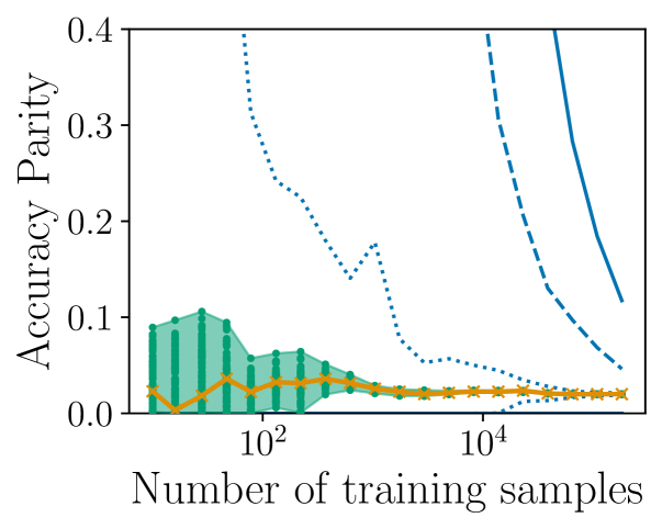
(a) Accuracy Parity (celebA)

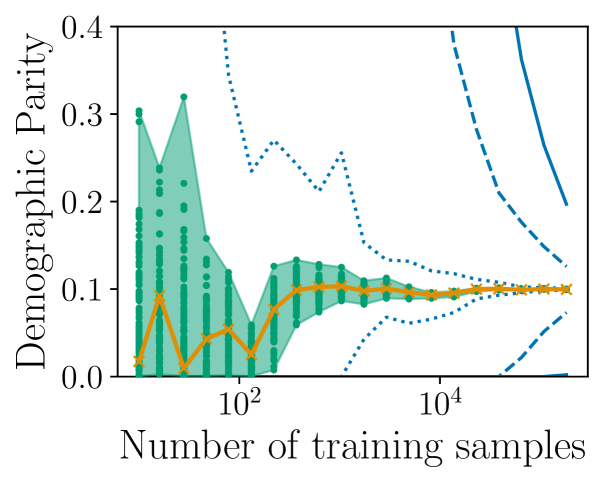
(b) Demographic Parity (celebA)

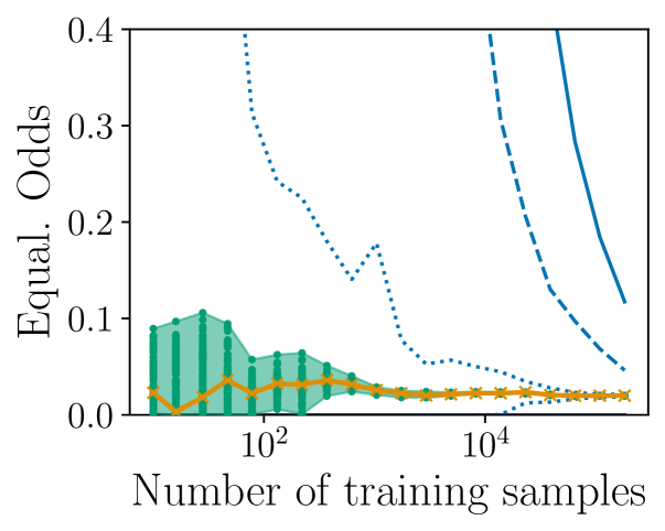
(c) Equalized Odds (celebA)

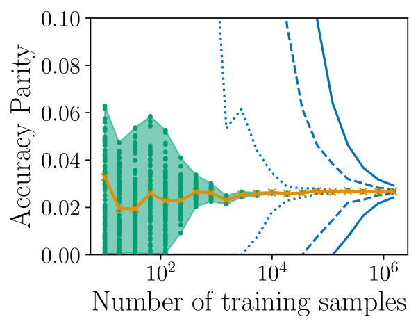
(d) Accuracy Parity (folktables)

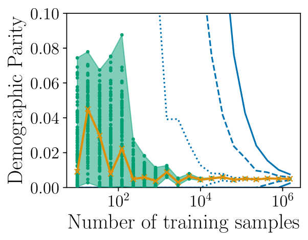
(e) Demographic Parity (folktables)

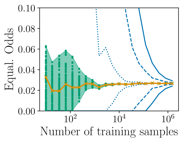
(f) Equalized Odds (folktables)

Figure 2: Fairness and accuracy levels for optimal non-private model and random private ones as a function of the number $n$ of training samples. For each value of $n$, we sample $100$ private models and take their minimum and maximum fairness/accuracy values to mark the area of attainable values. The solid blue line and the dashed one give our guarantees, respectively from Theorem 4.4 with Lemma 4.1’s bounds and with an empirical evaluation of $\left\|h^{\text{priv}}-h^{*}\right\|$.

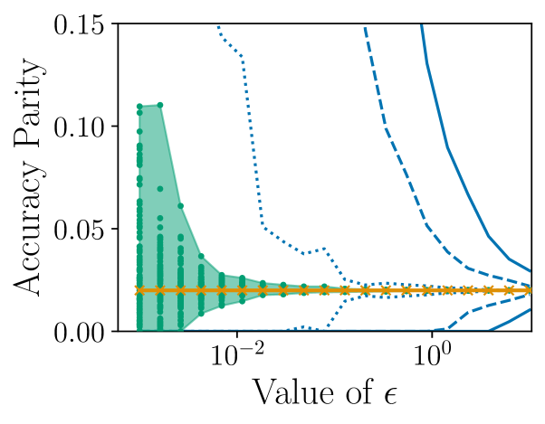
(a) Accuracy Parity (celebA)

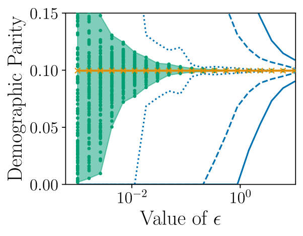
(b) Demographic Parity (celebA)

(c) Equality of Opportunity (celebA)

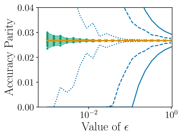
(d) Accuracy Parity (folktables)

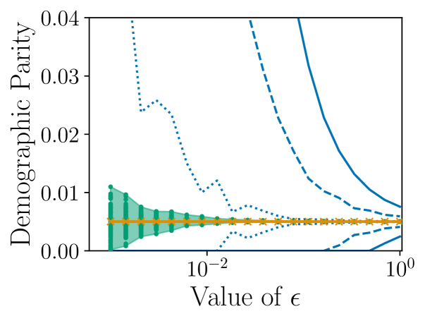
(e) Demographic Parity (folktables)

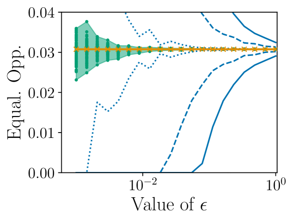
(f) Equality of Opportunity (folktables)

Figure 3: Fairness and accuracy levels for optimal non-private model and random private ones as a function of privacy budget $\epsilon$. For each value of $\epsilon$, we sample $100$ private models and take their minimum and maximum fairness/accuracy values to mark the area of attainable values. The solid blue line and the dashed one respectively give our guarantees, respectively from Theorem 4.4 with Lemma 4.1’s bounds and with an empirical evaluation of $\left\|h^{\text{priv}}-h^{*}\right\|$.

G.3 Refined Bounds with Additional Knowledge of $\bm{h^{\mathrm{priv}}}$ and $\bm{h^{*}}$

In 2.1, we use a uniform Lipschitz bound for all $h,h^{\prime}\in\mathcal{H}$. Let’s consider the class $\mathcal{H}$ of linear models, where, for $h\in\mathcal{H}$, we denote by $h_{y}$ the parameters of $h$ associated with the label $y$, that is $h(x,y)=h_{y}^{T}x$. For linear models, we derived the bound $\left\|\rho(h,x,y)-\rho(h^{\prime},x,y)\right\|_{\mathcal{H}}\leq 2\left\|x\right\|_{2}\left\|h-h^{\prime}\right\|_{\mathcal{H}}$, as derived in Section 2. Note that this inequality can be very loose whenever $x$ and $h_{y}-h_{y}^{\prime}$ (for $y\in\mathcal{Y}$) are (close to) orthogonal. When they are orthogonal, this bounds only gives $0=(h_{y}-h_{y}^{\prime})^{T}x\leq\left\|h_{y}-h_{y}^{\prime}\right\|_{2}\left\|x\right\|_{2}$. We can thus improve the inequality by remarking that we have

$$\left|\rho(h,x,y)-\rho(h^{\prime},x,y)\right|\leq{} \left|h(x,y)-h^{\prime}(x,y)\right|+\max_{y^{\prime}\neq y}\left|h(x,y^{\prime})-h^{\prime}(x,y^{\prime})\right|$$

$$={} \left|h_{y}^{T}x-h_{y}^{\prime T}x\right|+\max_{y^{\prime}\neq y}\left|h_{y^{\prime}}^{T}x-h^{\prime}_{y^{\prime}}x\right|$$

$$={} \left|(h_{y}-h_{y}^{\prime})^{T}x\right|+\max_{y^{\prime}\neq y}\left|(h_{y^{\prime}}-h^{\prime}_{y^{\prime}})x\right|$$

$$={} \left|(h_{y}-h_{y}^{\prime})^{T}p_{h_{y}-h^{\prime}_{y}}(x)\right|+\max_{y^{\prime}\neq y}\left|(h_{y^{\prime}}-h^{\prime}_{y^{\prime}})p_{h_{y}-h^{\prime}_{y}}(x)\right|$$

$$\leq{} 2\max_{y^{\prime}\in\mathcal{Y}}\left\|p_{h_{y}-h_{y}^{\prime}}(x)\right\|\left\|h-h^{\prime}\right\|_{\mathcal{H}}\enspace,$$

where $p_{h_{y}-h^{\prime}_{y}}(x)$ is the projection of $x$ on the axis defined by $h_{y}-h^{\prime}_{y}$. We can thus define a variant of $L_{X,Y}$ which depends on $h-h^{\prime}$

$$L_{X,Y}^{h-h^{\prime}}=2\max_{y\in\mathcal{Y}}\left\|p_{h_{y}-h_{y}^{\prime}}(x)\right\|\enspace.$$ (38)

Replacing 2.1 by this inequality in the proof of Theorem 3.1, we end up with the inequality

$$\left|\operatorname*{\mathbb{P}}\left(H(X)=Y\;\middle|\;E\right)-\operatorname*{\mathbb{P}}\left(H^{\prime}(X)=Y\;\middle|\;E\right)\right|\leq{}\operatorname*{\mathbb{P}}\left(\frac{\left|\rho(h,X,Y)\right|}{L_{X,Y}^{h-h^{\prime}}}\leq\left\|h-h^{\prime}\right\|_{\mathcal{H}}\;\middle|\;E\right)\enspace,$$

where the probability is over $(X,S,Y)\sim\mathcal{D}$. We obtained the same bound as Theorem 3.1, except with $L_{X,Y}^{h-h^{\prime}}$ instead of $L_{X,Y}$. Note that even if this gives a much tighter bound, this can generally not be computed, as one of $h$ or $h^{\prime}$ is typically not known.

References

• Abadi et al. (2016) Abadi, M., Chu, A., Goodfellow, I., McMahan, H. B., Mironov, I., Talwar, K., and Zhang, L. Deep Learning with Differential Privacy. In Proceedings of the 2016 ACM SIGSAC Conference on Computer and Communications Security, CCS ’16, pp.  308–318, New York, NY, USA, October 2016. Association for Computing Machinery. 1130 citations (Crossref) [2022-08-19].
• Agarwal (2020) Agarwal, S. Trade-offs between fairness and privacy in machine learning. 2020.
• Bagdasaryan et al. (2019) Bagdasaryan, E., Poursaeed, O., and Shmatikov, V. Differential privacy has disparate impact on model accuracy. In Advances in Neural Information Processing Systems 32, 2019, Vancouver, BC, Canada, pp.  15453–15462, 2019.
• Bassily et al. (2014) Bassily, R., Smith, A., and Thakurta, A. Private Empirical Risk Minimization: Efficient Algorithms and Tight Error Bounds. In 2014 IEEE 55th Annual Symposium on Foundations of Computer Science, pp.  464–473, Philadelphia, PA, USA, October 2014. IEEE.
• Bassily et al. (2022) Bassily, R., Mohri, M., and Suresh, A. T. Differentially private learning with margin guarantees. arXiv preprint arXiv:2204.10376, 2022.
• Bechavod & Ligett (2017) Bechavod, Y. and Ligett, K. Penalizing unfairness in binary classification. arXiv preprint arXiv:1707.00044, 2017.
• Beimel et al. (2014) Beimel, A., Brenner, H., Kasiviswanathan, S. P., and Nissim, K. Bounds on the sample complexity for private learning and private data release. Machine Learning, pp.  401–437, March 2014.
• Calders et al. (2009) Calders, T., Kamiran, F., and Pechenizkiy, M. Building classifiers with independency constraints. In 2009 IEEE International Conference on Data Mining Workshops, pp.  13–18. IEEE, 2009.
• Caton & Haas (2020) Caton, S. and Haas, C. Fairness in machine learning: A survey. arXiv preprint arXiv:2010.04053, 2020.
• Chang & Shokri (2020) Chang, H. and Shokri, R. On the privacy risks of algorithmic fairness. arXiv preprint arXiv:2011.03731, 2020.
• Chaudhuri et al. (2011) Chaudhuri, K., Monteleoni, C., and Sarwate, A. D. Differentially Private Empirical Risk Minimization. Journal of Machine Learning Research, 12(29):1069–1109, 2011. ISSN 1533-7928.
• Cortes et al. (2013) Cortes, C., Mohri, M., and Rostamizadeh, A. Multi-class classification with maximum margin multiple kernel. In International Conference on Machine Learning, pp.  46–54. PMLR, 2013.
• Cummings et al. (2019) Cummings, R., Gupta, V., Kimpara, D., and Morgenstern, J. On the compatibility of privacy and fairness. In Adjunct Publication of the 27th Conference on User Modeling, Adaptation and Personalization, pp.  309–315, 2019.
• Ding et al. (2021) Ding, F., Hardt, M., Miller, J., and Schmidt, L. Retiring adult: New datasets for fair machine learning. Advances in Neural Information Processing Systems, 34, 2021.
• Dwork (2006) Dwork, C. Differential privacy. In Encyclopedia of Cryptography and Security, 2006.
• Dwork et al. (2012) Dwork, C., Hardt, M., Pitassi, T., Reingold, O., and Zemel, R. Fairness through awareness. In Proceedings of the 3rd innovations in theoretical computer science conference, pp.  214–226, 2012.
• Dwork et al. (2014) Dwork, C., Roth, A., et al. The algorithmic foundations of differential privacy. Foundations and Trends in Theoretical Computer Science, 9(3-4):211–407, 2014.
• Farrand et al. (2020) Farrand, T., Mireshghallah, F., Singh, S., and Trask, A. Neither private nor fair: Impact of data imbalance on utility and fairness in differential privacy. arXiv preprint arXiv:2009.06389, 2020.
• Fioretto et al. (2022) Fioretto, F., Tran, C., Hentenryck, P. V., and Zhu, K. Differential privacy and fairness in decisions and learning tasks: A survey. In International Joint Conference on Artificial Intelligence (IJCAI), pp.  5470–5477, 2022.
• Ganev et al. (2022) Ganev, G., Oprisanu, B., and Cristofaro, E. D. Robin hood and matthew effects: Differential privacy has disparate impact on synthetic data. In ICML, 2022.
• Hardt et al. (2016) Hardt, M., Price, E., and Srebro, N. Equality of opportunity in supervised learning. Advances in neural information processing systems, 29:3315–3323, 2016.
• Hastie et al. (2009) Hastie, T., Tibshirani, R., and Friedman, J. The Elements of Statistical Learning. Springer Series in Statistics. Springer, New York, NY, 2009. ISBN 978-0-387-84857-0 978-0-387-84858-7. doi: 10.1007/978-0-387-84858-7. URL http://link.springer.com/10.1007/978-0-387-84858-7.
• Huang & Vishnoi (2019) Huang, L. and Vishnoi, N. Stable and fair classification. In International Conference on Machine Learning, pp. 2879–2890. PMLR, 2019.
• Jagielski et al. (2019) Jagielski, M., Kearns, M., Mao, J., Oprea, A., Roth, A., Sharifi-Malvajerdi, S., and Ullman, J. Differentially private fair learning. In International Conference on Machine Learning, pp. 3000–3008. PMLR, 2019.
• Kasiviswanathan et al. (2011) Kasiviswanathan, S. P., Lee, H. K., Nissim, K., Raskhodnikova, S., and Smith, A. What Can We Learn Privately? SIAM Journal on Computing, pp.  793–826, January 2011.
• Kiefer (1953) Kiefer, J. Sequential minimax search for a maximum. Proceedings of the American mathematical society, 4(3):502–506, 1953.
• Kilbertus et al. (2018) Kilbertus, N., Gascón, A., Kusner, M., Veale, M., Gummadi, K., and Weller, A. Blind justice: Fairness with encrypted sensitive attributes. In International Conference on Machine Learning, pp. 2630–2639. PMLR, 2018.
• Kusner et al. (2017) Kusner, M. J., Loftus, J., Russell, C., and Silva, R. Counterfactual fairness. Advances in neural information processing systems, 30, 2017.
• Liu et al. (2021) Liu, B., Ding, M., Shaham, S., Rahayu, W., Farokhi, F., and Lin, Z. When machine learning meets privacy: A survey and outlook. ACM Computing Surveys (CSUR), 54(2):1–36, 2021.
• Liu et al. (2015) Liu, Z., Luo, P., Wang, X., and Tang, X. Deep learning face attributes in the wild. In Proceedings of International Conference on Computer Vision (ICCV), December 2015.
• Lohaus et al. (2020) Lohaus, M., Perrot, M., and Von Luxburg, U. Too relaxed to be fair. In International Conference on Machine Learning, pp. 6360–6369. PMLR, 2020.
• Lowy & Razaviyayn (2021) Lowy, A. and Razaviyayn, M. Output perturbation for differentially private convex optimization with improved population loss bounds, runtimes and applications to private adversarial training. arXiv preprint arXiv:2102.04704, 2021.
• Maheshwari & Perrot (2022) Maheshwari, G. and Perrot, M. Fairgrad: Fairness aware gradient descent. arXiv preprint arXiv:2206.10923, 2022.
• Mehrabi et al. (2021) Mehrabi, N., Morstatter, F., Saxena, N., Lerman, K., and Galstyan, A. A survey on bias and fairness in machine learning. ACM Computing Surveys (CSUR), 54(6):1–35, 2021.
• Mironov (2017) Mironov, I. Renyi Differential Privacy. 2017 IEEE 30th Computer Security Foundations Symposium (CSF), August 2017.
• Mozannar et al. (2020) Mozannar, H., Ohannessian, M., and Srebro, N. Fair learning with private demographic data. In International Conference on Machine Learning, pp. 7066–7075. PMLR, 2020.
• Pedregosa et al. (2011) Pedregosa, F., Varoquaux, G., Gramfort, A., Michel, V., Thirion, B., Grisel, O., Blondel, M., Prettenhofer, P., Weiss, R., Dubourg, V., Vanderplas, J., Passos, A., Cournapeau, D., Brucher, M., Perrot, M., and Duchesnay, E. Scikit-learn: Machine learning in Python. Journal of Machine Learning Research, 12:2825–2830, 2011.
• Pujol et al. (2020) Pujol, D., McKenna, R., Kuppam, S., Hay, M., Machanavajjhala, A., and Miklau, G. Fair decision making using privacy-protected data. In Proceedings of the 2020 Conference on Fairness, Accountability, and Transparency, FAT* ’20, pp.  189–199, New York, NY, USA, 2020. Association for Computing Machinery. ISBN 9781450369367.
• Sanyal et al. (2022) Sanyal, A., Hu, Y., and Yang, F. How unfair is private learning? arXiv preprint arXiv:2206.03985, 2022.
• Shalev-Shwartz & Ben-David (2014) Shalev-Shwartz, S. and Ben-David, S. Understanding machine learning: From theory to algorithms. Cambridge university press, 2014.
• Song et al. (2013) Song, S., Chaudhuri, K., and Sarwate, A. D. Stochastic gradient descent with differentially private updates. In 2013 IEEE Global Conference on Signal and Information Processing, pp.  245–248, Austin, TX, USA, December 2013. IEEE. 145 citations (Crossref) [2022-08-19].
• Tran et al. (2020) Tran, C., Fioretto, F., and Van Hentenryck, P. Differentially private and fair deep learning: A lagrangian dual approach. arXiv preprint arXiv:2009.12562, 2020.
• Tran et al. (2021) Tran, C., Dinh, M., and Fioretto, F. Differentially private empirical risk minimization under the fairness lens. Advances in Neural Information Processing Systems, 34:27555–27565, 2021.
• Uniyal et al. (2021) Uniyal, A., Naidu, R., Kotti, S., Singh, S., Kenfack, P. J., Mireshghallah, F., and Trask, A. Dp-sgd vs pate: Which has less disparate impact on model accuracy? arXiv preprint arXiv:2106.12576, 2021.
• Woodworth et al. (2017) Woodworth, B., Gunasekar, S., Ohannessian, M. I., and Srebro, N. Learning non-discriminatory predictors. In Conference on Learning Theory, pp.  1920–1953. PMLR, 2017.
• Xu et al. (2019) Xu, D., Yuan, S., and Wu, X. Achieving differential privacy and fairness in logistic regression. In Companion Proceedings of The 2019 World Wide Web Conference, pp.  594–599, 2019.
• Xu et al. (2020) Xu, D., Du, W., and Wu, X. Removing disparate impact of differentially private stochastic gradient descent on model accuracy. arXiv preprint arXiv:2003.03699, 2020.
• Zafar et al. (2017) Zafar, M. B., Valera, I., Gomez Rodriguez, M., and Gummadi, K. P. Fairness beyond disparate treatment & disparate impact: Learning classification without disparate mistreatment. In Proceedings of the 26th international conference on world wide web, pp.  1171–1180, 2017.