Physics-Informed Convolutional Neural Networks for Corruption Removal on Dynamical Systems

Abstract

Measurements on dynamical systems, experimental or otherwise, are often subjected to inaccuracies capable of introducing corruption; removal of which is a problem of fundamental importance in the physical sciences. In this work we propose physics-informed convolutional neural networks for stationary corruption removal, providing the means to extract physical solutions from data, given access to partial ground-truth observations at collocation points. We showcase the methodology for 2D incompressible Navier-Stokes equations in the chaotic-turbulent flow regime, demonstrating robustness to modality and magnitude of corruption.

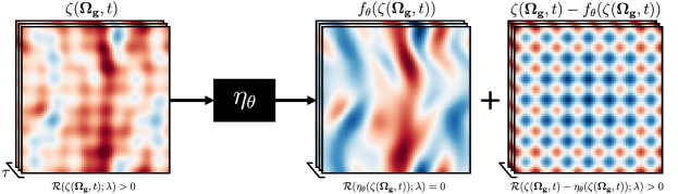
Figure 1: Diagrammatic overview of the corruption removal task.

1 Introduction

In the physical sciences, corrupted data can arise for a number of reasons: faulty experimental sensors, or low-fidelity numerical results to name a few. The detection and removal of this corruption would allow for the extraction of the underlying true-state, ensuring that the governing equations are satisfied. In practice, verifying that given observations are characteristic of a dynamical system is more straightforward than determining the solution itself. For observations on dynamical systems we evaluate the residual, giving an indication of the fidelity of the observations.

Corruption removal typically considers noise-removal, and flow-reconstruction [1]. Noise-removal constitutes methods which remove small, stochastic variations from the true-state, with examples including: filtering methods [2], proper orthogonal decomposition [3, 4], and autoencoders [5]. Flow-reconstruction considers inference of a solution over the domain, given only partial information; a popular example being that of super-resolution. Convolutional neural networks (CNNs) are prominent in the domain of flow reconstruction due to their ability to exploit spatial correlations [6, 7].

In the absence of ground-truth labels, it is possible to impose prior knowledge by regularising predictions with respect to known governing equations [8]. Physics-informed CNNs have been used for solving PDEs [9, 10], basic super-resolution [11], and surrogate modelling without access to labelled data [12]. This regularisation method differs from the standard physics-informed neural network (PINN) approach which strives to exploit the automatic-differentiation capabilities of neural networks to constrain gradients of the network [13].

Our work considers a form of physics-informed CNNs for flow reconstruction. We provide a method for removing arbitrary, stationary corruption from observations on dynamical systems, given access to only partial ground-truth information at select collocation points. We showcase corruption removal for the 2D incompressible Navier-Stokes equations in the chaotic-turbulent regime, highlighting the ability to accurately recover the true-state, independent of modality or magnitude of corruption.

2 Methodology

We consider corruption removal from observations on dynamical systems of the form

$$\partial_{t}\bm{u}-\mathcal{N}(\bm{u};\lambda)=0\qquad\text{with}\quad\bm{u}=u(\bm{x},t),\quad\bm{x}\in\Omega\subset\mathbb{R}^{n},\quad t\in[0,T]\subset\mathbb{R}^{+},$$ (1)

where $u:\Omega\times[0,T]\rightarrow\mathbb{R}^{n}$, $\mathcal{N}$ is a sufficiently smooth differential operator, and $\lambda$ are the physical parameters of the system. We define the residual of the system as the left-hand side of equation (1)

$$\mathcal{R}(\bm{u};\lambda)\triangleq\partial_{t}\bm{u}-\mathcal{N}(\bm{u};\lambda),$$ (2)

such that $\mathcal{R}(\bm{u};\lambda)=0$ when $u(\bm{x},t)$ is a solution to the partial differential equation (PDE). We consider corrupted observations such that $\mathcal{R}(\zeta(\bm{x},t);\lambda)>0$, where $\zeta(\bm{x},t)$ is the linear combination of the true state $u(\bm{x},t)$ and the stationary corruption $\phi(\bm{x})$, precisely $\zeta(\bm{x},t)=u(\bm{x},t)+\phi(\bm{x}).$

Given the corrupted state, we aim to recover the underlying, physical solution to the governing equations: the true-state. Mathematically, we denote this process by the mapping

$$\eta_{\theta}:\zeta(\bm{\Omega_{g}},t)\rightarrow u(\bm{\Omega_{g}},t),$$ (3)

where the domain $\Omega$ is discretised on a uniform, structured grid $\bm{\Omega_{g}}\subset\mathbb{R}^{N^{n}}$. We further discretise the time domain, providing $\mathcal{T}=\{t_{i}\in[0,T]\}_{i=0}^{N_{t}}$ for $N_{t}$ samples in time. Approximating the mapping $\eta_{\theta}$ as a CNN, we optimise weights of the network to minimise the loss

$$\mathcal{L}_{\theta}=\alpha\left(\mathcal{L}_{\partial\Omega}+\mathcal{L}_{\phi}\right)+\mathcal{L}_{\mathcal{R}},$$ (4)

where $\alpha$ is a fixed, empirical weighting factor. We define each of the loss terms as

$$\mathcal{L}_{\mathcal{R}} =\frac{1}{\lvert\mathcal{T}\rvert}\sum_{t\in\mathcal{T}}\big{\lVert}\mathcal{R}\big{(}\eta_{\theta}(\zeta(\bm{\Omega_{g}},t));\lambda\big{)}\big{\rVert}_{\bm{\Omega_{g}}}^{2},$$ (5)

$$\mathcal{L}_{\partial\Omega} =\frac{1}{\lvert\mathcal{T}\rvert}\sum_{t\in\mathcal{T}}\big{\lVert}\eta_{\theta}(\zeta(\partial\bm{\Omega_{g}},t))-u(\partial\bm{\Omega_{g}},t)\big{\rVert}_{\partial\bm{\Omega_{g}}}^{2},$$ (6)

$$\mathcal{L}_{\phi} =\frac{1}{\lvert\mathcal{T}\rvert}\sum_{t\in\mathcal{T}}\big{\lVert}\partial_{t}\big{[}\zeta(\bm{\Omega_{g}},t)-\eta_{\theta}(\zeta(\bm{\Omega_{g}},t))\big{]}\big{\rVert}_{\bm{\Omega_{g}}}^{2},$$ (7)

where $\partial\bm{\Omega_{g}}$ denotes boundary points of the grid, and $\lVert\mathrel{\;\cdot\;}\rVert_{\Omega}$ is the $\ell^{2}$-norm over the given domain. We regularise network predictions with the residual-based loss $\mathcal{L}_{\mathcal{R}}$, imposing prior-knowledge of the system to promote network realisations which conform to the governing equations. The data-driven boundary loss $\mathcal{L}_{\partial\Omega}$ serves to minimise the error between predictions and known measurements; when used in conjunction with the residual-loss, this effectively allows us to condition the underlying physics on the observations. For this case, we consider access to ground-truth measurements on the boundary $\partial\Omega$. Inclusion of the corruption-based loss $\mathcal{L}_{\phi}$ embeds our assumption of stationary corruption, driving predictions away from the trivial solution, $u(\bm{\Omega_{g}},t)=0$.

3 Results

We consider the corruption removal for measurements on the Kolmogorov flow, an instance of the 2D incompressible Navier-Stokes equations. The flow is defined on the domain $\Omega\in[0,2\pi)\subset\mathbb{R}^{2}$, imposing periodic boundary conditions on $\partial\Omega$, and subjected to stationary, sinusoidal forcing $g(\bm{x})$. The chaotic-turbulent nature of the Kolmogorov flow provides a challenging case study, introducing complex non-linear dynamics and turbulent structures across a range of spatial frequencies [14]. The standard continuity and momentum equations are given as

$$\begin{split}\nabla\cdot\bm{u}&=0\\ \partial_{t}\bm{u}+\bm{u}\cdot\nabla\bm{u}&=-\nabla p+\nu\Delta\bm{u}+g(\bm{x}),\end{split}$$ (8)

where $p,\nu$ denote the scalar pressure field and kinematic viscosity respectively. We take $\nu=\nicefrac{{1}}{{34}}$ to ensure chaotic-turbulent dynamics, and prescribe the forcing model $g(\bm{x})=[\sin(4\bm{x}_{2}),0]^{\top}$.

3.1 Pseudospectral Discretisation

We provide a differentiable pseudospectral discretisation for the differential operator, defining operations on the spectral grid $\bm{\hat{\Omega}_{k}}\in\mathbb{Z}^{61\times 61}$, enabling backpropagation for the residual-based loss $\mathcal{L}_{\mathcal{R}}$. By eliminating the pressure term, our discretisation handles the continuity constraint implicitly, affording us the ability to neglect the constraint in the loss [15]. We produce a solution by time-integration of the dynamical system with the forward-Euler method, taking a time-step $\Delta t=0.005$ to ensure numerical stability according to the Courant-Friedrichs-Levy condition.

Due to the spectral discretisation, we evaluate the residual-based loss $\mathcal{L}_{\mathcal{R}}$ in the Fourier domain on the grid $\bm{\hat{\Omega}_{k}}$, offering two distinct advantages over the standard finite-difference approach: spectral accuracy, and implicit handling of periodic boundary conditions. We employ a form of time-windowed batching, considering the evaluation of the residual-based loss over $\tau\geq 2$ consecutive time-steps.

3.2 Parameterised Corruption

We conduct experiments varying the frequency $f$, and relative magnitude $\mathcal{M}$ of the corruption. For a scaling magnitude $M=\mathcal{M}\cdot\max{\left(u(\bm{\Omega_{g}},\mathrel{\;\cdot\;})\right)}$, we define the corruption field as

$$\phi(\bm{x};f,M)=\Gamma\left(20+\sum_{i=1}^{2}\left[(\bm{x}_{i}-\pi)^{2}-10\cos(f\cdot(\bm{x}_{i}-\pi))\right];M\right),$$ (9)

where $\Gamma(\;\bm{\cdot}\;;M)$ is a linear operator that re-scales the vector in the range $[0,M]$, [16].

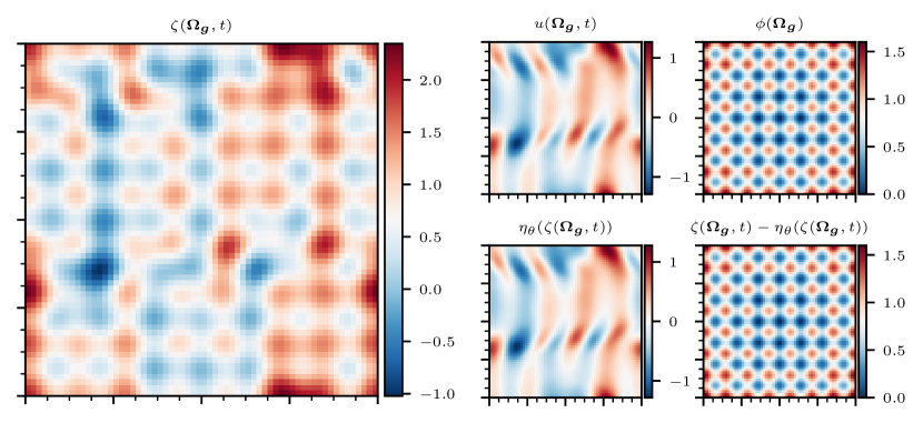
Figure 2: Corruption removal results for the Kolmogorov flow $[f=7,\mathcal{M}=0.5]$.

3.3 Numerical Experiments

The Kolmogorov flow is solved in the Fourier domain, as per §3.1, before generating data on the grid $\bm{\Omega_{g}}\in\mathbb{R}^{64\times 64}$. A total of $1024$ time-windows are used for training, with a further $256$ for validation, taking $\tau=2$ in each instance. We employ a standard U-Net [17] architecture and train with the Adam optimizer, taking a learning rate of $3\times 10^{-4}$ for $5000$ epochs, fixing computational resource for each experiment. We impose a fixed weighting of $\alpha=1\times 10^{3}$ for the empirical weighting term.

In Figure 2 we demonstrate results for $f=7,\mathcal{M}=0.5$, showcasing the ability to separate the true-state from corruption. We note that the residual of the corruption is not equal to the sum of the residuals of it’s constituents, highlighting the challenge of non-linearity. We further assess the robustness of the methodology to both modality and magnitude of corruption by running two studies:

$$\begin{aligned} &\mathit{(i)}\\ &\mathit{(ii)}\end{aligned}\quad\begin{aligned} &\mathcal{M}=0.5,\\ &f=3,\end{aligned}\quad\begin{aligned} f&\in\{1,3,5,7,9\};\\ \mathcal{M}&\in\{0.01,0.1,0.25,0.5,1.0\}.\end{aligned}$$

Results can be seen in Figure 3, where performance for all experiments is measured by the relative $\ell^{2}$-error between the predicted-state $\eta_{\theta}(\zeta(\bm{\Omega}_{g},t))$, and the true-state $u(\bm{\Omega_{g}},t)$. Results denote the mean over five repeats with random seeds, the standard deviation not exceeding $8.169\times 10^{-4}$.

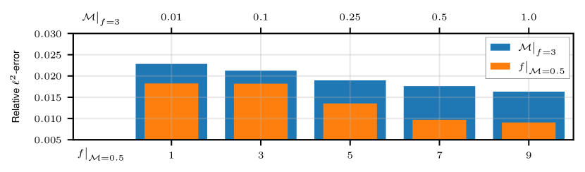
Figure 3: Comparison of relative $\ell^{2}$-error for parameterised corruption frequency and magnitude.

We find that performance is largely agnostic to both multi-modality and magnitude of corruption, with error decreasing slightly with increasing $f,\mathcal{M}$, as demonstrated in Figure 3. Quantitatively, we observe excellent robustness of the methodology, with relative $\ell^{2}$-error not exceeding $2.284\times 10^{-2}$.

4 Conclusion

In this work we introduce a methodology for physics-informed removal of arbitrary, stationary corruption from observations on dynamical systems, given access to only partial ground-truth information. We demonstrate results for corrupted observations on the Kolmogorov flow, using ground-truth observations on the boundaries to condition the physics. Experiments indicate that performance is agnostic to both magnitude and modality of corruption, with relative $\ell^{2}$-error remaining consistently low, as demonstrated in Figure 3. Our results in Figure 2 qualitatively showcase the performance of the model, clearly separating the corrupted field into its component parts: true-state, and corruption. This work opens opportunities for accurate flow reconstruction from corrupted state measurements with access to partial ground-truth information, potentially allowing for correcting sensor measurements and low-fidelity simulation results - problems of fundamental importance in the physical sciences.

We note the limitations of our work: the assumption of stationary corruption, and the requirement of ground-truth observations to condition the physics; providing considerations for future work.

References

- Brunton et al. [2020] S. Brunton, B. Noack, and P. Koumoutsakos, “Machine learning for fluid mechanics,” Annual Review of Fluid Mechanics, vol. 52, pp. 477–508, 1 2020.
- Kumar and Nachamai [2017] N. Kumar and M. Nachamai, “Noise removal and filtering techniques used in medical images,” Oriental journal of computer science and technology, vol. 10, pp. 103–113, 3 2017.
- Raiola et al. [2015] M. Raiola, S. Discetti, and A. Ianiro, “On piv random error minimization with optimal pod-based low-order reconstruction,” Experiments in Fluids, vol. 56, 4 2015.
- Mendez et al. [2017] M. A. Mendez, M. Raiola, A. Masullo, S. Discetti, A. Ianiro, R. Theunissen, and J. M. Buchlin, “Pod-based background removal for particle image velocimetry,” Experimental Thermal and Fluid Science, vol. 80, pp. 181–192, 1 2017.
- Vincent et al. [2008] P. Vincent, H. Larochelle, Y. Bengio, and P.-A. Manzagol, “Extracting and composing robust features with denoising autoencoders,” in Proceedings of the 25th International Conference on Machine Learning, 2008, pp. 1096–1103.
- Dong et al. [2014] C. Dong, C. C. Loy, K. He, and X. Tang, “Learning a deep convolutional network for image super-resolution,” in European Conference on Computer Vision, 2014, pp. 184–199.
- Shi et al. [2016] W. Shi, J. Caballero, F. Huszár, J. Totz, A. P. Aitken, R. Bishop, D. Rueckert, and Z. Wang, “Real-time single image and video super-resolution using an efficient sub-pixel convolutional neural network,” Computer Vision and Pattern Recognition, 9 2016.
- Lagaris et al. [1998] I. E. Lagaris, A. Likas, and D. I. Fotiadis, “Artificial neural networks for solving ordinary and partial differential equations,” IEEE Transactions on Neural Networks, vol. 9, pp. 987–1000, 1998.
- Gao et al. [2021a] H. Gao, L. Sun, and J. X. Wang, “Phygeonet: Physics-informed geometry-adaptive convolutional neural networks for solving parameterized steady-state pdes on irregular domain,” Journal of Computational Physics, vol. 428, 3 2021.
- Ren et al. [2022] P. Ren, C. Rao, Y. Liu, J. X. Wang, and H. Sun, “Phycrnet: Physics-informed convolutional-recurrent network for solving spatiotemporal pdes,” Computer Methods in Applied Mechanics and Engineering, vol. 389, 2 2022.
- Gao et al. [2021b] H. Gao, L. Sun, and J.-X. Wang, “Super-resolution and denoising of fluid flow using physics-informed convolutional neural networks without high-resolution labels,” Physics of Fluids, vol. 33, p. 073603, 7 2021.
- Zhao et al. [2021] X. Zhao, Z. Gong, Y. Zhang, W. Yao, and X. Chen, “Physics-informed convolutional neural networks for temperature field prediction of heat source layout without labeled data,” Preprint, 9 2021. [Online]. Available: http://arxiv.org/abs/2109.12482
- Raissi et al. [2019] M. Raissi, P. Perdikaris, and G. E. Karniadakis, “Physics-informed neural networks: A deep learning framework for solving forward and inverse problems involving nonlinear partial differential equations,” Journal of Computational Physics, vol. 378, pp. 686–707, 2 2019.
- Fylladitakis [2018] E. D. Fylladitakis, “Kolmogorov flow: Seven decades of history,” Journal of Applied Mathematics and Physics, vol. 06, pp. 2227–2263, 2018.
- Canuto et al. [1988] C. Canuto, M. Y. Hussaini, A. Quarteroni, and T. A. Zang, Spectral Methods in Fluid Dynamics. Springer Berlin Heidelberg, 1988.
- Rastrigin [1974] L. A. Rastrigin, “Systems of extremal control,” Nauka, 1974.
- Ronneberger et al. [2015] O. Ronneberger, P. Fischer, and T. Brox, “U-net: Convolutional networks for biomedical image segmentation,” in Medical Image Computing and Computer-Assisted Intervention, 2015, pp. 234–241.