Preferential Subsampling for Stochastic Gradient Langevin Dynamics

Abstract

Stochastic gradient MCMC (SGMCMC) offers a scalable alternative to traditional MCMC, by constructing an unbiased estimate of the gradient of the log-posterior with a small, uniformly-weighted subsample of the data. While efficient to compute, the resulting gradient estimator may exhibit a high variance and impact sampler performance. The problem of variance control has been traditionally addressed by constructing a better stochastic gradient estimator, often using control variates. We propose to use a discrete, non-uniform probability distribution to preferentially subsample data points that have a greater impact on the stochastic gradient. In addition, we present a method of adaptively adjusting the subsample size at each iteration of the algorithm, so that we increase the subsample size in areas of the sample space where the gradient is harder to estimate. We demonstrate that such an approach can maintain the same level of accuracy while substantially reducing the average subsample size that is used.

Keywords Stochastic gradient MCMC  $\cdot$ Langevin dynamics  $\cdot$ Scalable MCMC  $\cdot$ Control variates

1 Introduction

Markov chain Monte Carlo (MCMC) algorithms are a popular family of methods to conduct Bayesian inference. Unfortunately, running MCMC on large datasets is generally computationally expensive, which often limits the use of MCMC by practitioners. The Metropolis-Hastings algorithm (Metropolis et al., 1953; Hastings, 1970), in particular, requires a scan of the full dataset at each iteration to calculate the acceptance probability.

Stochastic gradient Markov chain Monte Carlo (SGMCMC) algorithms are a family of scalable methods, which aim to address this issue (Welling and Teh, 2011; Nemeth and Fearnhead, 2021). These algorithms aim to leverage the efficiency of gradient-based MCMC proposals (Roberts and Tweedie, 1996; Neal, 2011). They reduce the per-iteration computational cost by constructing an unbiased, noisy estimate of the gradient of the log-posterior, using only a small data subsample. In this paper, we focus on samplers that rely on the overdamped Langevin diffusion (Roberts and Tweedie, 1996), however, our proposed methodology can be applied more generally to other SGMCMC algorithms, such as those based on Hamiltonian dynamics (Chen et al., 2014).

The high variance inherently present in the stochastic gradient estimator can degrade sampler performance and lead to poor convergence. As such, variance control has become an important area of research within the SGMCMC literature, and is often required to make these algorithms practical (Dubey et al., 2016; Chatterji et al., 2018; Baker et al., 2019; Chen et al., 2019).

In this paper, we propose a new method designed to reduce the variance in the stochastic gradient. We use a discrete, non-uniform probability distribution to preferentially subsample data points and to re-weight the stochastic gradient. In addition, we present a method for adaptively adjusting the size of the subsample chosen at each iteration.

2 Stochastic gradient MCMC

Let $\theta\in\mathbb{R}^{d}$ be a parameter vector and denote independent observations $\mathbf{x}=\{x_{i}\}_{i=1}^{N}$ ($N\gg 1$). The probability density of the $i$-th observation, given parameter $\theta$, is $p(x_{i}|\theta)$ and the prior density for the parameters is $p(\theta)$. In a Bayesian context, the target of interest is the posterior density, $\pi(\theta)\vcentcolon=p(\theta|\mathbf{x})\propto p(\theta)\prod_{i=1}^{N}p(x_{i}|\theta).$

For convenience, we define $f_{i}(\theta)=-\log p(x_{i}|\theta)$ for $i=1,\ldots,N$, with $f_{0}(\theta)=-\log p(\theta)$ and $f(\theta)=f_{0}(\theta)+\sum_{i=1}^{N}f_{i}(\theta)$. In this setting, the posterior density can be rewritten as, $\pi(\theta)\propto\exp(-f(\theta))$.

2.1 The Langevin diffusion

The Langevin diffusion, $\theta(t)$, is defined by the stochastic differential equation,

$$d\theta(t)=-\frac{1}{2}\nabla f(\theta(t))dt+dB_{t},$$ (1)

where $\nabla f(\theta(t))dt$ is a drift term and $B_{t}$ denotes a $d$-dimensional Wiener process. Under certain regularity conditions, the stationary distribution of this diffusion is the posterior $\pi$ (Roberts and Tweedie, 1996). In practice, we need to discretise Eq. (1) in order to simulate from it and this introduces error. For a small step-size $\epsilon>0$, the Langevin diffusion can be approximated by

$$\theta^{(t+1)}=\theta^{(t)}-\frac{\epsilon}{2}\nabla f\big{(}\theta^{(t)}\big{)}+\sqrt{\epsilon}\,\eta^{(t)},$$ (2)

where the noise $\eta^{(t)}\sim\mathcal{N}_{d}(\mathbf{0},I_{d\times d})$ is drawn independently at each update. The dynamics implied by Eq. (2) provide a simple way to sample from the Langevin diffusion. The level of discretisation error in the approximation is controlled by the size of $\epsilon$ and we can achieve any required degree of accuracy if we choose $\epsilon$ small enough.

The unadjusted Langevin algorithm (ULA) (Parisi, 1981) is a simple sampler that simulates from Eq. (2) but does not use a Metropolis-Hastings correction (Metropolis et al., 1953; Hastings, 1970). Thus, the samples obtained from ULA produce a biased approximation of $\pi$. The per-iteration computational cost of ULA is smaller than that of the Metropolis-adjusted Langevin algorithm (Roberts and Rosenthal, 1998) due to the removal of the Metropolis-Hastings step. However, the computational bottleneck for ULA lies in the $O(N)$ calculation of the full data gradient $\nabla f\big{(}\theta^{(t)}\big{)}=\nabla f_{0}\big{(}\theta^{(t)}\big{)}+\sum_{i=1}^{N}\nabla f_{i}\big{(}\theta^{(t)}\big{)}$ at every iteration. This calculation can be problematic if $N$ is large.

2.2 Stochastic gradient Langevin dynamics

The stochastic gradient Langevin dynamics (SGLD) algorithm attempts to improve the per-iteration computational burden of ULA by replacing the full-data gradient with an unbiased estimate (Welling and Teh, 2011). Let the full-data gradient of $f(\theta)$ be given by

$$g^{(t)}=\nabla f\big{(}\theta^{(t)}\big{)}=\nabla f_{0}\big{(}\theta^{(t)}\big{)}+\sum_{i=1}^{N}\nabla f_{i}\big{(}\theta^{(t)}\big{)}.$$

The unbiased estimate of $g^{(t)}$ proposed by Welling and Teh (2011) takes the form

$$\hat{g}^{(t)}=\nabla f_{0}\big{(}\theta^{(t)}\big{)}+\frac{N}{n}\sum_{i\in\mathcal{S}^{t}}\nabla f_{i}\big{(}\theta^{(t)}\big{)},$$ (3)

where $\mathcal{S}^{t}$ is a subset of $\{1,\ldots,N\}$ and $|\mathcal{S}^{t}|=n$ ($n\ll N$) is the subsample size. A single update of SGLD is thus given by,

$$\theta^{(t+1)}\leftarrow\theta^{(t)}-\frac{\epsilon^{(t)}}{2}\cdot\hat{g}^{(t)}+\xi^{(t)},$$ (4)

where $\xi^{(t)}\sim\mathcal{N}_{d}(0,\epsilon^{(t)}I_{d\times d})$ and $\{\epsilon^{(t)}\}$ corresponds to a schedule of step-sizes which may be fixed (Vollmer et al., 2016) or decreasing (Teh et al., 2016). The full SGLD pseudocode is provided in Algorithm 1.

Algorithm 1 SGLD

1:  Input: initialise $\theta^{(1)}$, batch size $n$, step-sizes $\{\epsilon^{(t)}\}$.

2:  for $t=1,2,\ldots,T$ do

3:     Sample indices $S^{t}\subset\{1,\ldots,N\}$ with or without replacement.

4:     Calculate $\hat{g}^{(t)}$ using Eq. (3).

5:     Update parameters according to Eq. (4).

6:  end for

7:  return  $\theta^{(T+1)}$

Welling and Teh (2011) note that if the step-size $\epsilon^{(t)}\rightarrow 0$ as $t\rightarrow\infty$, then the Gaussian noise (generated by $\xi^{(t)}$) dominates the noise in the stochastic gradient term. For large $t$, the algorithm approximately samples from the posterior using an increasingly accurate discretisation of the Langevin diffusion. In practice, SGLD does not mix well when the step-size is decreased to zero and so a small fixed step-size $\epsilon$ is typically used instead.

2.3 Control variates for SGLD

The naive stochastic gradient proposed by Welling and Teh (2011) may exhibit a relatively high variance for small subsamples of data. The more faithful a stochastic gradient estimator is to the full-data gradient, the better we can expect SGLD to perform. Therefore, it is natural to consider alternatives to the estimator given in Eq. (3) which minimise the variance.

Let $\hat{\theta}$ be a fixed value of the parameter, typically chosen to be close to the mode of the target posterior density. The control variate gradient estimator proposed by Baker et al. (2019) takes the form,

$$\hat{g}_{cv}^{(t)}=\big{[}\nabla f(\hat{\theta})+\nabla f_{0}\big{(}\theta^{(t)}\big{)}-\nabla f_{0}(\hat{\theta})\big{]}\,+\,$$ (5)

$$\frac{N}{n}\sum_{i\in\mathcal{S}^{t}}\big{[}\nabla f_{i}\big{(}\theta^{(t)}\big{)}-\nabla f_{i}(\hat{\theta})\big{]}.$$

When $\theta^{(t)}$ is close to $\hat{\theta}$, the variance of the gradient estimator will be small. This is shown formally in Lemma 1 of Baker et al. (2019).

The SGLD-CV algorithm is the same as SGLD given in Algorithm 1, except with $\hat{g}_{cv}^{(t)}$ substituted in place of $\hat{g}^{(t)}$. Implementing the SGLD-CV estimator involves a one-off pre-processing step to find $\hat{\theta}$, which is typically done using stochastic gradient descent (SGD) (Bottou et al., 2018; Baker et al., 2019). The gradient terms $\nabla f_{i}\big{(}\hat{\theta})$ are calculated and stored. While these steps are both $O(N)$ in computational cost, the optimisation step to find the mode can replace the typical burn-in phase of the SGLD chain. The MCMC chain can then be initialised at the posterior mode itself. The full pseudocode for SGLD-CV is provided in Algorithm 3 within Appendix B.

3 Preferential data subsampling

Let $\mathcal{S}$ be a subsample of size $n$ generated with replacement, such that the probability that the $i$-th data point, $x_{i}$, appears in $\mathcal{S}$ is $p_{i}$. The expected number of times $x_{i}$ is drawn from the dataset is $np_{i}$. A standard implementation of SGLD would assume uniform subsampling, i.e. that $p_{i}=\frac{1}{N}$ for all $i$. However, if the observations vary in their information about the parameters, then assigning a larger probability to the more informative observations would be advantageous. Preferential subsampling assigns a strictly-positive, user-chosen weight to each data point, such that we minimise the variance of the estimator of the gradient.

We need to construct a discrete probability distribution $\mathbf{p}^{(t)}=(p_{1}^{t},\ldots,p_{N}^{t})^{T}$ (where $p_{i}^{(t)}>0$ for all $i$ and $\sum_{i}p_{i}^{t}=1$) that can be used to draw subsamples of size $n$ at each iteration $t$ and to reweight the stochastic gradient accordingly. If $\mathbf{p}^{(t)}$ is time-invariant (i.e. $p_{i}^{(t)}=p_{i}$ for all $i$), the preferential subsampling scheme is static. Otherwise, the subsampling weights will be dynamic or state-dependent.

For a given stochastic gradient $\tilde{g}$, the noise term associated with $\tilde{g}$ is given by $\xi^{(t)}=\tilde{g}^{(t)}-g^{(t)}$. Taking expectations over $\mathbf{p}^{(t)}$, a simple scalar summary of the variance of the noise $\xi^{(t)}$ can be found by evaluating:

$$\mathbb{E}\,\bigg{(}\big{\|}\xi^{(t)}\big{\|}^{2}\bigg{)}=\operatorname{tr}\bigg{(}\operatorname{Cov}\big{(}\tilde{g}^{(t)}\big{)}\bigg{)}.$$ (6)

We will refer to Eq. (6) as the pseudo-variance of $\tilde{g}^{(t)}$, $\mathbb{V}\big{(}\tilde{g}^{(t)}\big{)}$, from now on. We intend to use the pseudo-variance as a proxy for the variance of the stochastic gradient. In all further analysis, $\|\cdot\|$ refers to the Euclidean norm.

In order to minimise the pseudo-variance, we need to find a preferential subsampling distribution $\mathbf{p}^{*}$ which minimises the following problem:

$$\min_{\mathbf{p}^{(t)},\,p_{i}^{t}\in[0,1],\sum_{i}p_{i}^{t}=1}\mathbb{V}\big{(}\tilde{g}^{(t)}\big{)}.$$ (7)

Existing non-asymptotic convergence results for SGLD-type methods demonstrate the importance in controlling the variance of the stochastic gradient. These results give the error of SGLD in terms of bounds on the (bias and) variance of the estimator of the gradient of the log posterior. Therefore, constructing a better stochastic gradient estimator - for instance via preferential subsampling - will lead to a reduction in the error bound of the underlying SGLD method.

3.1 SGLD with preferential subsampling

An alternative gradient estimator for SGLD can be given by reweighting the simple estimator defined in Eq. (3) (Welling and Teh, 2011),

$$\tilde{g}^{(t)}=\nabla f_{0}\big{(}\theta^{(t)}\big{)}+\frac{1}{n}\sum_{i\in\mathcal{S}^{t}}\frac{1}{p_{i}^{t}}\nabla f_{i}\big{(}\theta^{(t)}\big{)},$$ (8)

where $S^{t}\subset\{1,\ldots,N\}$ is selected according to $\mathbf{p}^{(t)}$ and $|S^{t}|=n\enspace(n\ll N)$. The pseudocode for the SGLD with preferential subsampling (SGLD-PS) algorithm is outlined in Algorithm 4 within Appendix B.

As we correct for the non-uniform subsampling of data points by reweighting each gradient term, it follows that the stochastic gradient estimator given in Eq. (8) is unbiased. This is synonymous with the standard properties of importance sampling estimators (Robert and Casella, 2004). We note that there is an extra $O(n)$ computational cost associated with reweighting the stochastic gradient in this manner at each iteration.

The following result obtains the optimal solution to Problem (7).

Lemma 3.1.

For the unbiased SGLD-PS gradient estimator in Eq. (8), minimising Problem (7) is equivalent to minimising the following

$$\min_{\mathbf{p}^{(t)}}\frac{1}{n}\sum_{i=1}^{N}\frac{1}{p_{i}^{t}}\big{\|}\nabla f_{i}\big{(}\theta^{(t)}\big{)}\big{\|}^{2}.$$ (9)

The optimal weights which minimise the pseudo-variance are thus given by

$$p_{i}^{t}=\frac{\|\nabla f_{i}\big{(}\theta^{(t)}\big{)}\|}{\sum_{k=1}^{N}\|\nabla f_{k}\big{(}\theta^{(t)}\big{)}\|}\,\text{ for }i=1,\ldots,N.$$ (10)

Although a solution to Eq. (9) can be found, the resulting sampling algorithm would not be practical, as the optimal weights depend on the current state $\theta^{(t)}$. Therefore the subsampling distribution given in Eq. (10) requires $N$ gradient calculations per iteration. For large datasets, these weights would be very expensive to store and calculate at each iteration, making the algorithm impractical.

We can instead approximate the optimal weights given in Eq. (10), such that they are not state-dependent and therefore do not need to be updated at each iteration. These approximate weights can be calculated as an initial pre-processing step before the main sampling algorithm is run.

A fairly simple approximation of the optimal weights given in Eq. (10) for SGLD-PS would require substituting the current state $\theta^{(t)}$ with some alternative fixed point. The posterior mode, $\hat{\theta}$, is a sensible choice as it represents the most probable estimate of the parameters in a Bayesian paradigm. In this case, the approximate subsampling scheme would be given by,

$$p_{i}=\frac{\|\nabla f_{i}\big{(}\hat{\theta}\big{)}\|}{\sum_{k=1}^{N}\|\nabla f_{k}\big{(}\hat{\theta}\big{)}\|}\,\text{ for }i=1,\ldots,N.$$ (11)

As with SGLD-CV, the posterior mode could be estimated using SGD and the MCMC chain could then be initialised at the posterior mode.

In practice, the subsampling weights in Eq. (11) are calculated only once with an $O(N)$ preprocessing step and then used statically (i.e without update). The resulting SGLD-PS algorithm would calculate the stochastic gradient given in Eq. (8) using these fixed weights.

3.2 SGLD-CV with preferential subsampling

The control-variates gradient estimator can be modified to accommodate a preferential subsampling scheme in a similar manner. In this case, we would obtain

$$\tilde{g}^{(t)}=\big{[}\nabla f(\hat{\theta})+\nabla f_{0}\big{(}\theta^{(t)}\big{)}-\nabla f_{0}(\hat{\theta})\big{]}\,+\,$$ (12)

$$\frac{1}{n}\sum_{i\in\mathcal{S}^{t}}\frac{1}{p_{i}^{t}}\big{[}\nabla f_{i}\big{(}\theta^{(t)}\big{)}-\nabla f_{i}(\hat{\theta})\big{]}.$$

The pseudocode for the modified SGLD-CV algorithm (SGLD-CV-PS) is given in Algorithm 5 within Appendix B. The following result provides the optimal solution to Problem (7).

Lemma 3.2.

For the unbiased SGLD-CV-PS gradient estimator in Eq. (12), minimising Problem (7) is equivalent to minimising the following

$$\min_{\mathbf{p}^{(t)}}\frac{1}{n}\sum_{i=1}^{N}\frac{1}{p_{i}^{t}}\big{\|}\nabla f_{i}\big{(}\theta^{(t)}\big{)}-\nabla f_{i}(\hat{\theta})\big{\|}^{2}.$$ (13)

The optimal weights which minimise the pseudo-variance are thus given by

$$p_{i}^{t}=\frac{\|\nabla f_{i}\big{(}\theta^{(t)}\big{)}-\nabla f_{i}(\hat{\theta}))\|}{\sum_{k=1}^{N}\|\nabla f_{k}\big{(}\theta^{(t)}\big{)}-\nabla f_{k}(\hat{\theta})\|}$$ (14)

for $i=1,\ldots,N$.

As in Section 3.1, we can derive a solution to Eq. (13). However, the resulting sampling algorithm would once again depend on the current state of the chain $\theta^{(t)}$. The process of finding a suitable approximation to the optimal weights given in Eq. (14) for the control-variate gradient estimator is non-trivial. Our approach will be to choose a set of subsampling weights that could be used for all iterations of the MCMC chain.

We consider an alternative minimisation problem

$$\min_{\mathbf{p}^{(t)},\,p_{i}^{t}\in[0,1],\sum_{i}p_{i}^{t}=1}\mathbb{E}_{\theta}\bigg{[}\mathbb{V}\big{(}\tilde{g}^{(t)}\big{)}\bigg{]},$$ (15)

where the outer expectation is taken with respect to the posterior distribution. Due to the linearity of expectation, Eq. (15) is equivalent to solving the following problem:

$$\min_{\mathbf{p}^{(t)}}\mathbb{E}_{\theta}\bigg{[}\frac{1}{n}\sum_{i=1}^{N}\frac{1}{p_{i}^{t}}\big{\|}\nabla f_{i}\big{(}\theta^{(t)}\big{)}-\nabla f_{i}(\hat{\theta})\big{\|}^{2}\bigg{]}.$$

This can easily be shown by using a modified version of the argument given for Lemmas 3.1 and 3.2. The optimal subsampling weights in Eq. (14) can be approximated by

$$p_{i}\propto\sqrt{\text{tr}\bigg{(}\nabla^{2}f_{i}(\hat{\theta})\,\hat{\Sigma}\,\nabla^{2}f_{i}(\hat{\theta})^{T}\bigg{)}}\text{ for }i=1,\ldots,N,$$ (16)

where $\nabla^{2}f_{i}(\cdot)$ is the Hessian matrix of $f_{i}(\cdot)$ and $\hat{\Sigma}$ is the covariance matrix of the Gaussian approximation to the target posterior centred at the mode.

See Appendix A.4 for a full discussion of how these weights can be obtained analytically and Appendix D for an assessment of the computational cost associated with calculating them as a preprocessing step. The computational cost required to calculate the Hessian matrix means that this approach can be computationally expensive for high-dimensional parameters.

3.3 Adaptive subsampling

In this section, we present a method for adaptively adjusting the size of the subsample chosen at each iteration. We do this by first finding an upper bound for the pseudo-variance of the stochastic gradient estimator given in Eq. (12) and then by rearranging the result to find a lower bound on the subsample size.

Let us begin by placing a Lipschitz condition on each of the likelihood terms.

Assumption 1.

(Lipschitz continuity of gradients)
There exists constants $L_{0},\ldots,L_{N}$ such that

$$\|\nabla f_{i}(\theta)-\nabla f_{i}(\theta^{\prime})\|\leq L_{i}\|\theta-\theta^{\prime}\|$$ (17)

for $i=0,\ldots,N$.

We can then obtain the following result using Assumption 1.

Lemma 3.3.

Under Assumptions 1, the pseudo-variance of the stochastic gradient estimator defined in Eq. (12) can be bounded above by

$$\mathbb{V}(\tilde{g})\leq\frac{1}{n}\|\theta^{(t)}-\hat{\theta}\|^{2}\bigg{(}\sum_{i=1}^{N}\frac{L_{i}^{2}}{p_{i}^{t}}\bigg{)}\,.$$ (18)

where $\mathbf{p}^{(t)}=(p_{1}^{t},\ldots,p_{N}^{t})^{T}$ is a set of user-defined discrete weights.

We can minimise the upper bound provided in Eq. (18) if we plug in the optimal weights given in Eq. (14). In practice, however, it is advantageous to choose the preferential subsampling scheme based on its ease of computation.

The bound provided in Lemma 3.3 can still be used more generally to control the size of the pseudo-variance of the stochastic gradient estimator given in Eq. (12). If we want to set the upper threshold of the pseudo-variance to be some fixed value $V_{0}>0$, we need to ensure that

$$\frac{1}{n}\|\theta^{(t)}-\hat{\theta}\|^{2}\bigg{(}\sum_{i=1}^{N}\frac{L_{i}^{2}}{p_{i}^{t}}\bigg{)}<V_{0},\,$$

for all iterations $t=1,\ldots,T$. We can rearrange the inequality above to obtain the following lower bound on the subsample size,

$$n>\frac{1}{V_{0}}\|\theta^{(t)}-\hat{\theta}\|^{2}\bigg{(}\sum_{i=1}^{N}\frac{L_{i}^{2}}{p_{i}^{t}}\bigg{)}.$$ (19)

For a given preferential subsampling scheme $\mathbf{p}^{(t)}$, we can control the noise of the stochastic gradient estimator given in Eq. (12) by choosing the subsample size $n\propto\|\theta^{(t)}-\hat{\theta}\|^{2}$. This means that the subsample size can be set adaptively according to the current state of the chain.

Our proposed algorithm is provided in Algorithm 2. The subsample size at iteration $t$, $n^{(t)}$, will be updated using the lower bound obtained in Eq. (19). For a fixed noise threshold $V_{0}$, it will be possible to decrease or increase the size of $n^{(t)}$ depending on how far or close $\theta^{(t)}$ is to the posterior mode, $\hat{\theta}$.

This method is suitable for use on models that satisfy Assumption 1. Appendix C provides a selection of examples where the Lipschitz constants can be calculated exactly.

Algorithm 2 Adaptive SGLD-CV with preferential subsampling (ASGLD-CV-PS)

1:  Input: initialise $\theta^{(1)}$ close to $\hat{\theta}$, gradients $\nabla f_{i}\big{(}\hat{\theta})$, weights $\mathbf{p}^{(1)}$, step-size $\epsilon$, noise threshold $V_{0}$, Lipschitz constants $\{L_{i}\}_{i=1}^{N}$.

2:  for $t=1,2,\ldots,T$ do

3:     Update $\mathbf{p}^{(t)}$.

4:     Find smallest possible $n^{(t)}$ using Eq. (19).

5:     Sample $n^{(t)}$ indices $\mathcal{S}^{t}$ according to $\mathbf{p}^{(t)}$ with replacement.

6:     Calculate $\tilde{g}^{(t)}$ using Eq. (12)

7:     Update parameters according to Eq. (4).

8:  end for

9:  return  $\theta^{(T+1)}$

4 Related work

The idea of using a non-uniform discrete distribution to draw subsamples and reweight a gradient estimator has been well-explored within the stochastic optimisation literature. Typically, the aim of these methods is to control the variance of the gradient estimator, in order to improve the speed of convergence of the algorithm.

Various papers explore the use of a static or time-invariant subsampling schemes. Zhao and Zhang (2014b, 2015) and Kern and Gyorgy (2016) propose the use of an importance sampling approach for SGD-type algorithms, where the subsampling weights are chosen according to the Lipschitz smoothness constants of $N$ individual cost functions, i.e. $p_{i}=\frac{L_{i}}{\sum_{j=1}^{N}L_{j}}$. Zhao and Zhang (2014a) consider a stratified sampling approach, where data points are assigned the the same weight if they belong to the same strata or cluster. Zhang et al. (2017) propose the use of determinantal point processes to diversify the subsamples selected for SGD, constructing a soft similarity measure to reweight data points.

Inspired by active learning methods, Salehi et al. (2017) create a multi-armed bandit (MAB) framework to dynamically update the subsampling weights over several iterations of the SGD algorithm. Feedback is collected via the most recent stochastic gradients and passed into the MAB at each iteration. Liu et al. (2020) adapts the work of Salehi et al. and extends it to the minibatch setting for the ADAM algorithm (Kingma and Ba, 2016).

There have only been a handful of papers considering similar ideas within the stochastic gradient MCMC literature. Fu and Zhang (2017) extend the stratified sampling methodology of Zhao and Zhang (2014a) to the general class of SGMCMC algorithms. Li et al. (2021) meanwhile propose an exponentially weighted stochastic gradient method, which can be combined with other variance reduction techniques.

5 Numerical experiments

In the experiments to follow, we compare our proposed preferential subsampling approaches in a number of different scenarios. Our aim here is to demonstrate the value of preferential subsampling as a variance control measure. To communicate the idea succinctly, we only include the benchmark methods SGLD and SGLD-CV in our results.

We evaluate the performance of our proposed methods on both real and synthetic data. Please refer to Appendix C for detailed information about the datasets considered.

A fixed step-size scheme for $\epsilon$ is used throughout, as suggested by Vollmer et al. (2016). To ensure a fair comparison, all samplers were run with the same step-size (with $\epsilon\approx\frac{1}{N}$). This allowed us to control for discretisation error and to independently assess the performance benefits offered by preferential subsampling. See Appendix E for further details.

For samplers where the burn-in phase is replaced by an optimiser, we have opted to use an off-the-shelf implementation of ADAM (Kingma and Ba, 2016) to find the posterior mode. Unless stated otherwise, all samplers are implemented using sampling with replacement.

Computing environment

We used the jax autograd module to implement the SGMCMC methods. Our results were obtained on a four-core 3.00GHz Intel Xeon(R) Gold virtual desktop. The code for this paper is hosted on GitHub.

5.1 Models

We compare sampler performance on the following three models: (i) bivariate Gaussian, (ii) binary logistic regression and (iii) linear regression. Full model details (including the derivation gradients and Lipschitz constants) are provided in Appendix C.

The examples have been deliberately chosen to be simple and our reasons for doing so are threefold. Firstly, our proposed methods rely upon being able to estimate the posterior mode well and as such, we are prioritising models where the mode is easy to find. Secondly, the Lipschitz constants for these models are known and this allows us to test our adaptive subsampling approach. And lastly, the SGLD-CV-PS subsampling scheme outlined in Eq. (16) requires the Hessian matrix, $\nabla^{2}f_{i}(\cdot)$, to be computed for all data points and this is a costly preprocessing step for large parameter spaces.

5.1.1 Bivariate Gaussian

We simulate independent data from $X_{i}|\theta\sim\mathcal{N}_{2}(\theta,\Sigma_{x})$ for $i=1,\ldots,N.$ It is assumed that $\theta$ is unknown and $\Sigma_{x}$ is known. The conjugate prior for $\theta$ is set to be $\theta\sim\mathcal{N}_{2}(\mu_{0},\Lambda_{0}).$ The prior hyperparameters of the prior are $\mu_{0}=(0,0)^{T}$and $\Lambda_{0}=\mbox{diag}(1\times 10^{3},2)$. The target posterior is a non-isotropic Gaussian with negatively correlated parameters.

5.1.2 Binary logistic regression

Suppose we have data $x_{1},\dots,x_{N}$ of dimension $d$ taking values in $\mathbb{R}^{d}$, where each $x_{i}=(1,x_{i1},\ldots,x_{ip})^{T}$ (where $d=p+1$). Let us suppose that we also have the corresponding response variables $y_{1},\dots,y_{N}$ taking values in $\{0,1\}$. Then a logistic regression model with parameters $\theta=(\beta_{0},\beta_{1},\ldots,\beta_{p})$ will have the following density function

$$p(y_{i}|x_{i},\theta)=\bigg{(}\frac{1}{1+e^{-\theta^{T}x_{i}}}\bigg{)}^{y_{i}}\bigg{(}1-\frac{1}{1+e^{-\theta^{T}x_{i}}}\bigg{)}^{1-y_{i}}.$$

The prior for $\theta$ is set to be $\theta\sim\mathcal{N}_{d}(\mu_{0},\Lambda_{0}).$ The hyperparameters of the prior are $\mu_{0}=(0,\ldots,0)^{T}$ and $\Lambda_{0}=\mbox{diag}(10,d)$.

5.1.3 Linear regression

Suppose we have data $x_{1},\dots,x_{N}$ of dimension $d$ taking values in $\mathbb{R}^{d}$, where each $x_{i}=(1,x_{i1},\ldots,x_{ip})^{T}$ ($d=p+1$). Let us suppose that we also have the corresponding response variables $y_{1},\dots,y_{N}$ taking values on the real line.

We define the following linear regression model,

$$y_{i}=x_{i}^{T}\theta+\eta_{i},\enspace\eta_{i}\sim\mathcal{N}(0,1),$$

with parameters $\theta=(\beta_{0},\beta_{1},\ldots,\beta_{p})$. The prior for $\theta$ is the same as above.

5.2 Metrics

We assess the performance of our samplers using the following metrics.

5.2.1 Kullbeck-Leibler (KL) divergence

The KL divergence is a measure of difference between two probability distributions with densities $p(\cdot)$ and $q(\cdot)$ and is given by,

$$D_{KL}(p||q)=\int p(\theta)\log\frac{p(\theta)}{q(\theta)}d\theta.$$

In the case of our bivariate Gaussian model, we know that the target posterior is conjugate and the KL divergence between two Gaussians can be written analytically. We use the KL divergence to measure the difference between the target posterior and our generated samples in Figure 4(a).

5.2.2 Log-loss

The log-loss is a popular metric for assessing the predictive accuracy of the logistic regression model on a test dataset, $\mathcal{T}^{*}$. For binary classification, the log-loss is given by

$$l(\theta,\mathcal{T}^{*})=-\frac{1}{|\mathcal{T}^{*}|}\sum_{i\in|\mathcal{T}^{*}|}\log p(y_{i}^{*}|x_{i}^{*},\theta).$$

We compute the log-loss for our logistic regression example in Figure 2(b)(ii).

5.2.3 Kernel Stein discrepancy

We measure the sample quality of our MCMC chains using the kernel Stein discrepancy (KSD). The KSD assesses the discrepancy between the target posterior $\pi$ and the empirical distribution $\tilde{\pi}_{K}$ formed by SGMCMC samples $\{\theta\}_{k=1}^{K}$ (Liu et al., 2016; Gorham and Mackey, 2017). A key benefit of the KSD is that it penalises the bias present in our MCMC chains. We can define the KSD as,

$$KSD(\tilde{\pi}_{K},\pi)=\sum_{j=1}^{d}\sqrt{\sum_{k,k^{\prime}=1}^{K}\frac{k_{j}^{0}(\theta_{k},\theta_{k^{\prime}})}{K^{2}}},$$ (20)

where the Stein kernel for $j\in\{1,\ldots,d\}$ is given by,

$$k_{j}^{0}(\theta,\theta^{\prime})=\frac{1}{\pi(\theta)\pi(\theta^{\prime})}\nabla_{\theta_{j}}\nabla_{\theta^{\prime}_{j}}\big{(}\pi(\theta)\mathcal{K}(\theta,\theta^{\prime})\pi(\theta^{\prime})\big{)}$$ (21)

and $\mathcal{K}(\cdot,\cdot)$ is a valid kernel function. Gorham and Mackey (2017) recommend using the inverse multi-quadratic kernel, $\mathcal{K}(\theta,\theta^{\prime})=\big{(}c^{2}+\|\theta-\theta^{\prime}\|_{2}^{2}\big{)}^{\beta}$, which detects non-convergence for $c>0$ and $\beta\in(-1,0)$. In practice, the full-data gradients in Eq. (21) can be replaced by noisy, unbiased estimates. We compute the KSD for our linear and logistic regression examples in Figures 2(a) - (b)(i), 3(a), 4(b) and 5(a).

5.3 Numerical results

5.3.1 Evaluating the quality of the stochastic gradients

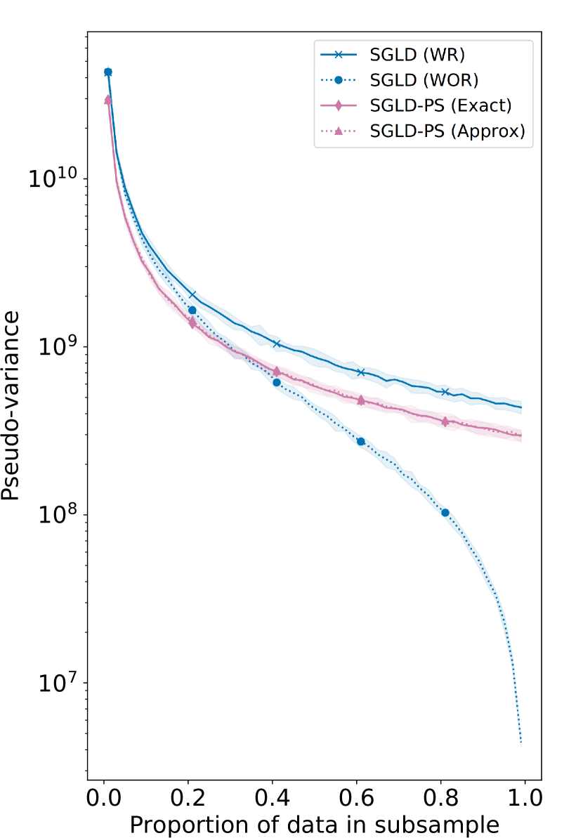
(a)

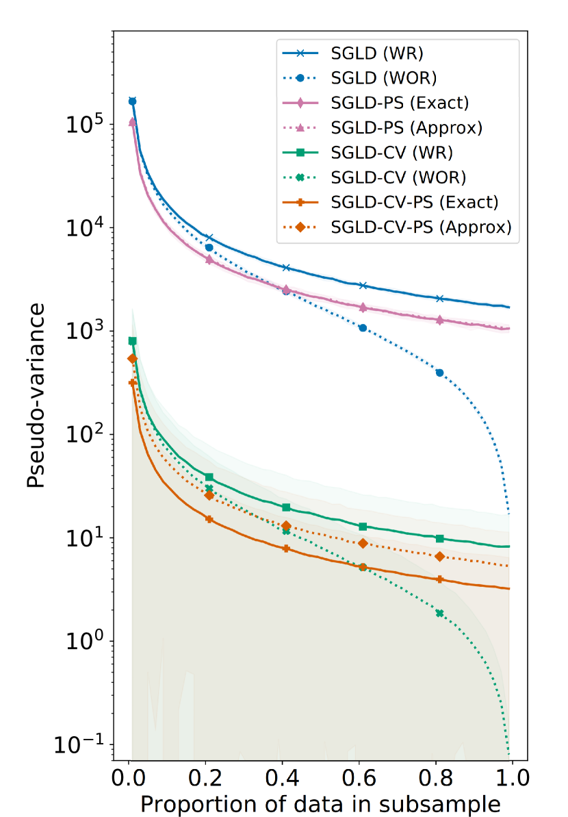
(b)

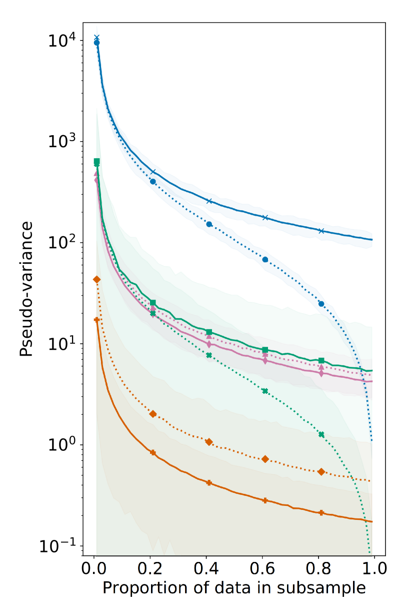
(c)

Figure 1: Empirical pseudo-variance against proportion of data in a subsample, $\frac{n}{N}$. (a) bivariate Gaussian, (b) balanced logistic regression, (c) imbalanced logistic regression

In this experiment, our objective was to compare the pseudo-variance of our proposed gradient estimators against the proportion of data used in a subsample, $\frac{n}{N}$. We consider three scenarios: (a) bivariate Gaussian (b) balanced bivariate logistic regression, and (c) imbalanced bivariate logistic regression. For ease of computation, a synthetic dataset of size $N=10^{3}$ was used for all models.

In each scenario, we generated ten candidate draws of $\theta$ and calculated an empirical estimate of the pseudo-variance at each. The candidate draws were sampled either from the posterior (for scenario (a)) or from a normal approximation to the posterior (for scenarios (b) and (c)). We plot the mean empirical estimate of the pseudo-variance for various subsample sizes.

Figure 1(a) compares the stochastic gradients for SGLD with and without replacement (WR and WOR respectively) and for SGLD-PS with exact and approximate subsampling schemes. Figures 1(b) and (c) additionally compare the gradient estimators of SGLD-CV and those of SGLD-CV-PS with exact and approximate subsampling schemes.

SGLD and SGLD-CV with replacement offer the best variance reduction for larger subsamples, as $\frac{n}{N}$ tends towards 1. For more reasonable subsample sizes of $n\leq 0.2N$, however, there is no major benefit in generating subsamples without replacement. Figure 1 illustrates that there is a marked reduction in the pseudo-variance when a preferential subsampling scheme is used.

SGLD-PS and SGLD-CV-PS consistently outperform their vanilla counterparts and there seems to be very little difference between the exact and approximate schemes for SGLD-PS. Whereas, there is a difference in performance between the exact and approximate subsampling schemes for SGLD-CV-PS. This difference is noticeable in Figure 1(c) for the synthetic imbalanced logistic regression data. Practically, it is not feasible to use the exact subsampling weights, but as illustrated here, using approximate preferential weights is always better than using uniform weights.

5.3.2 Performance of fixed subsample size methods

In Figure 2, we compare the sampler performance of SGLD, SGLD-CV, SGLD-PS and SGLD-CV-PS for a subsample size of 0.1% of the dataset size over 10 passes of the data. We have run ten MCMC chains allowing for an equal number of iterations for both burn-in and sampling.

Figure 2(a) plots the KSD results for the linear regression model fitted on the CASP dataset. The CASP dataset has been obtained from the UCI Machine Learning repository and contains 45,730 instances and 9 features.

Furthermore, Figure 2(b) plots the results of fitting the logistic regression model to the covertype dataset (Blackard and Dean, 1998). The covertype dataset contains 581,012 instances and 54 features. The KSD results are shown in Figure 2(b)(i) and the log-loss (evaluated every 10 iterations) is computed on the test set in Figure 2(b)(ii).

In addition, we separately compare the sampler performance of SGLD and SGLD-PS in Figure 4 (see Appendix F) for subsample sizes of $1\%$, $5\%$ and $10\%$ of the dataset size, over 500 passes of the data. As before, ten MCMC chains were run for each subsample size tested, allowing for an equal number of iterations for both burn-in and sampling

Figure 4(a) plots the KL divergence for the bivariate Gaussian model fitted on synthetic data of size $N=10^{4}$. Figure 4(b) plots the KSD for the logistic regression model fitted on the covertype dataset (Blackard and Dean, 1998).

We can see that SGLD-CV-PS exhibits the best performance overall. More generally, we find that there is a benefit in implementing preferential subsampling for vanilla SGLD as well. In practice, we find that the largest performance gains are found for preferential subsampling when the subsampling size is reasonably small.

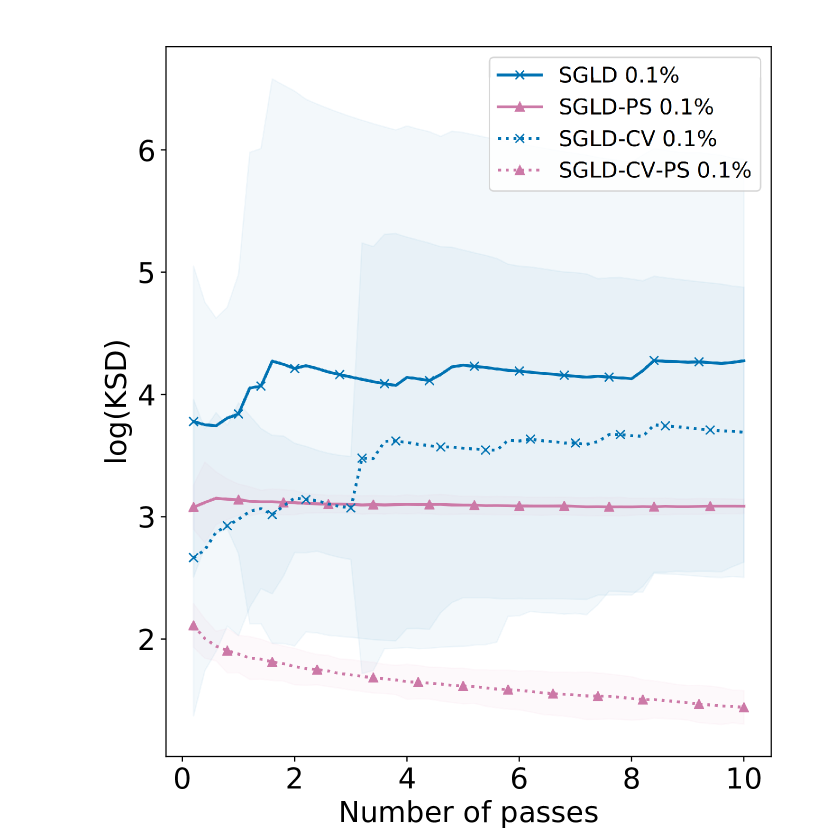
(a)

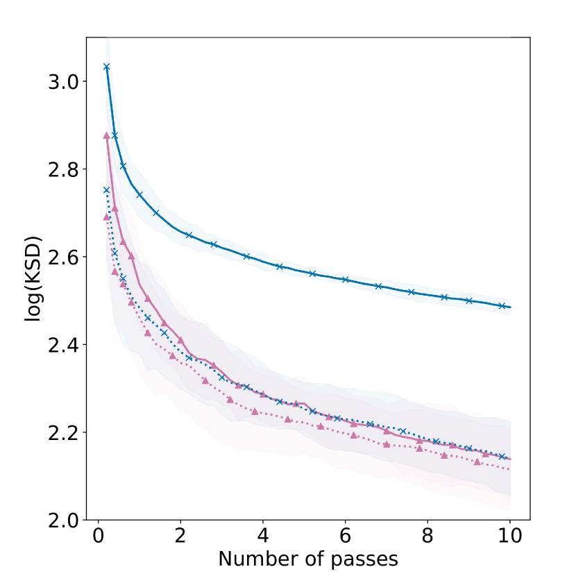
(b)(i)

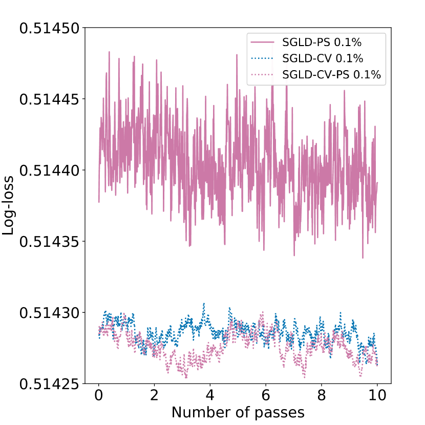
(b)(ii)

Figure 2: Sampler performance of SGLD, SGLD-CV, SGLD-PS and SGLD-CV-PS for 0.1% subsample size over 10 passes through the data. (a) linear regression model on the CASP data (y-axis: KSD); (b) logistic regression on the covertype data (y-axis: (i) KSD, (ii) log-loss).

5.3.3 Performance of adaptive subsampling

We are interested in assessing the sampler performance of ASGLD-CV and ASGLD-CV-PS over $10^{4}$ iterations. In this experiment, we considered two scenarios: (i) the logistic regression model on balanced synthetic data of size $N=10^{4}$; and (ii) the linear regression model on the CASP data. The results for scenario (i) are plotted in Figure 3. Please refer to Figure 5 in Appendix F for the results of scenario (ii). Both models satisfy Assumption 1.

In order to implement the adaptive subsampling methods, we had to first pick a suitable pseudo-variance threshold, $V_{0}$. We generated ten chains of SGLD-CV and SGLD-CV-PS for a fixed subsample of size 0.1% of the dataset size. For each chain, we then:

1. calculated the squared Euclidean distances between the mode and the samples, $\|\theta-\hat{\theta}\|^{2}$,

2. found the 95-th percentile of the array of squared distances, and

3. calculated a proposal for $V_{0}$ using the bound in Eq. (18).

We set $V_{0}$ to be the largest proposal amongst the ten chains.

Figure 3(a) plots the KSD for all four methods and Figure 3(b) displays the adaptive subsample sizes selected along one chain of ASGLD-CV-PS. Figure 3(c) compares the number of passes through the data considered by fixed subsampling versus ASGLD-CV-PS over $10^{4}$ iterations.

Overall, we see that the performance of ASGLD-CV-PS is somewhat better than that of ASGLD-CV. We cannot always presume that the adaptive subsampling methods will outperform their fixed subsampling counterparts (see Figure 5(a) for instance) in terms of sample quality. However, it is clear that the adaptive subsampling methods successfully process far less of the data over $10^{4}$ iterations with no significant reduction in statistical accuracy.

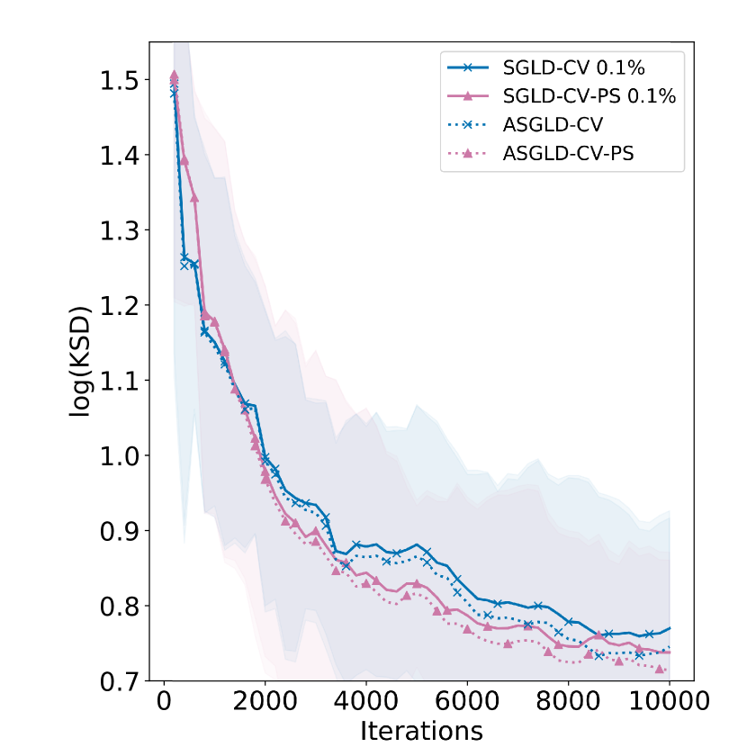
(a)

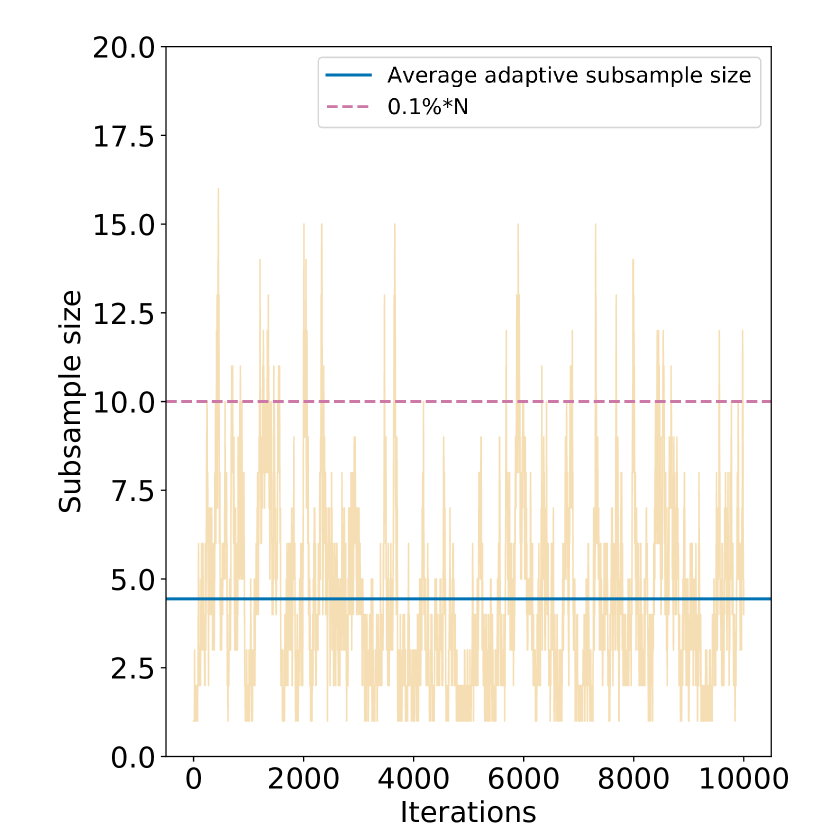
(b)

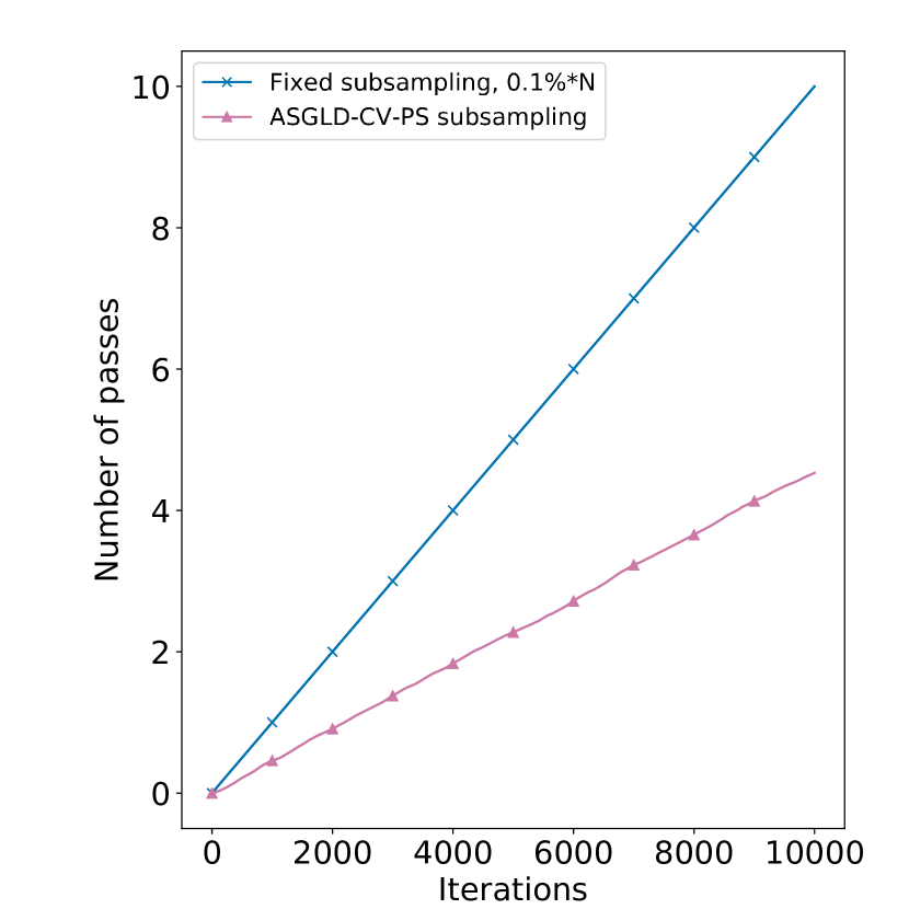
(c)

Figure 3: A logistic regression model fitted on balanced synthetic data of size $N=10^{4}$. (a) KSD comparison of SGLD-CV, SGLD-CV-PS, ASGLD-CV and ASGLD-CV-PS over $10^{4}$ iterations; (b) adaptive subsample sizes selected along one ASGLD-CV-PS chain; (c) the number of passes through the data considered by fixed versus adaptive subsampling.

6 Conclusion

We have used preferential subsampling to reduce the variance of the stochastic gradient estimator for both SGLD and SGLD-CV. In addition, we have extended SGLD-CV to allow for adaptive subsampling.

We have empirically studied the impact of preferential subsampling on a range of synthetic and real-world datasets. Our numerical experiments successfully demonstrate the performance improvement from both preferential subsampling and adaptively selecting the subsample size.

Future work in this area could explore the potential for using multi-armed bandits to preferentially select data subsamples for SGMCMC. These concepts have only been previously considered within the context of stochastic optimisation (Salehi et al., 2017; Liu et al., 2020).

The methods outlined in this paper are not limited to Langevin dynamics and can be applied to other SGMCMC samplers. Furthermore, it would be worth considering how preferential subsampling could be extended for other variance control methods, such as SAGA-LD or SVRG-LD (Dubey et al., 2016). This could potentially be done by adapting the ideas presented in Schmidt et al. (2015), Kern and Gyorgy (2016) and Schmidt et al. (2017). Arguments that mirror those presented in Lemmas 3.1 and 3.2 could be used to obtain the optimal preferential subsampling scheme in each new case.

Acknowledgements

SP gratefully acknowledges the support of the EPSRC funded EP/L015692/1 STOR-i Centre for Doctoral Training. CN acknowledges the support of EPSRC grants EP/S00159X/1, EP/V022636/1 and EP/R01860X/1. PF acknowledges support of EPSRC grants EP/N031938/1 and EP/R018561/1.SP gratefully acknowledges the support of the EPSRC funded EP/L015692/1 STOR-i Centre for Doctoral Training. CN acknowledges the support of EPSRC grants EP/V022636/1 and EP/R01860X/1. PF acknowledges support of EPSRC grants EP/N031938/1 and EP/R018561/1.

Appendix A Results from Section 3

A.1 Full derivation of the pseudo-variance

The pseudo-variance $\tilde{g}^{(t)}$ is given by:

$$\mathbb{V}\big{(}\tilde{g}^{(t)}\big{)} =\mathbb{E}\,\bigg{(}\big{\|}\tilde{g}^{(t)}-g^{(t)}\big{\|}^{2}\bigg{)}$$ (22)

$$=\mathbb{E}\,\bigg{(}\big{(}\tilde{g}^{(t)}-g^{(t)}\big{)}^{T}\big{(}\tilde{g}^{(t)}-g^{(t)}\big{)}\bigg{)}$$ (23)

$$=\sum_{j=1}^{d}\mathbb{E}\,\bigg{(}\big{(}\tilde{g}^{(t)}_{j}-g_{j}^{(t)}\big{)}^{2}\bigg{)}\text{\, \,\, \, \, (decompose expectation over $d$ parameters)}$$ (24)

$$=\sum_{j=1}^{d}\mathbb{E}\,\bigg{(}\big{(}\tilde{g}^{(t)}_{j}-\mathbb{E}\,\big{[}\,\tilde{g}^{(t)}_{j}\big{]}\big{)}^{2}\bigg{)}$$ (25)

$$=\sum_{j=1}^{d}\operatorname{Var}\big{(}\tilde{g}^{(t)}_{j}\big{)}$$ (26)

$$=\operatorname{tr}\bigg{(}\operatorname{Cov}\big{(}\tilde{g}^{(t)}\big{)}\bigg{)}.$$ (27)

A.2 Proof of Lemma 3.1

Proof.

From Section A.1, we know that

$$\mathbb{V}\big{(}\tilde{g}^{(t)}\big{)}=\mathbb{E}\,\Bigg{[}\big{\|}\tilde{g}^{(t)}-g^{(t)}\big{\|}^{2}\Bigg{]}=\sum_{j=1}^{d}\operatorname{Var}\big{(}\tilde{g}_{j}^{(t)}\big{)}.$$ (28)

Taking expectations with respect to $\mathbf{p}^{(t)}$, we know that the $j$-th component of the sum in Eq. (28) is given by:

$$\operatorname{Var}\big{(}\tilde{g}_{j}^{(t)}\big{)} =\operatorname{Var}\bigg{(}\nabla_{j}f_{0}\big{(}\theta^{(t)}\big{)}+\frac{1}{n}\sum_{i\in\mathcal{S}^{t}}\frac{1}{p_{i}^{t}}\nabla_{j}f_{i}\big{(}\theta^{(t)}\big{)}\bigg{)}=\operatorname{Var}\bigg{(}\frac{1}{n}\sum_{i\in\mathcal{S}^{t}}\frac{1}{p_{i}^{t}}\nabla_{j}f_{i}\big{(}\theta^{(t)}\big{)}\bigg{)}.$$

Given that all stochastic gradient estimators are unbiased with the same mean, we know that minimising $\mathbb{V}\big{(}\tilde{g}^{(t)}\big{)}$ with respect to $\mathbf{p}^{(t)}$ is equivalent to minimising the component-wise sum of second moments, $\sum_{j=1}^{d}\mathbb{E}\,\Bigg{(}\bigg{(}\frac{1}{n}\sum_{i\in\mathcal{S}^{t}}\frac{1}{p_{i}^{t}}\nabla_{j}f_{i}\big{(}\theta^{(t)}\big{)}\bigg{)}^{2}\Bigg{)}.$

So, for $j=1,\ldots,d$, we consider

$$\mathbb{E}\,\Bigg{(}\bigg{(}\frac{1}{n}\sum_{i\in\mathcal{S}^{t}}\frac{1}{p_{i}^{t}}\nabla_{j}f_{i}\big{(}\theta^{(t)}\big{)}\bigg{)}^{2}\Bigg{)} =\frac{1}{n^{2}}\,\mathbb{E}\,\Bigg{(}\sum_{i\in\mathcal{S}^{t}}\bigg{(}\frac{1}{p_{i}^{t}}\nabla_{j}f_{i}\big{(}\theta^{(t)}\big{)}\bigg{)}^{2}+\sum_{i\in\mathcal{S}^{t}}\sum_{k\in\mathcal{S}^{t},\,i\neq k}\frac{1}{p_{i}^{t}}\cdot\frac{1}{p_{k}^{t}}\cdot\nabla_{j}f_{i}\big{(}\theta^{(t)}\big{)}\cdot\nabla_{j}f_{k}\big{(}\theta^{(t)}\big{)}\Bigg{)}$$

$$=\frac{1}{n}\,\mathbb{E}\,\Bigg{(}\bigg{(}\frac{1}{p_{i}^{t}}\nabla_{j}f_{i}\big{(}\theta^{(t)}\big{)}\bigg{)}^{2}\Bigg{)}+\frac{n(n-1)}{n^{2}}\mathbb{E}\,\Bigg{(}\frac{1}{p_{i}^{t}}\nabla_{j}f_{i}\big{(}\theta^{(t)}\big{)}\Bigg{)}^{2}$$

$$=\frac{1}{n}\sum_{i=1}^{N}\frac{1}{p_{i}^{t}}\big{[}\nabla_{j}f_{i}\big{(}\theta^{(t)}\big{)}\big{]}^{2}+\frac{n-1}{n}\Bigg{(}\sum_{i=1}^{N}\nabla_{j}f_{i}\big{(}\theta^{(t)}\big{)}\Bigg{)}^{2}$$

$$=\frac{1}{n}\sum_{i=1}^{N}\frac{1}{p_{i}^{t}}\big{[}\nabla_{j}f_{i}\big{(}\theta^{(t)}\big{)}\big{]}^{2}+C_{j},$$

where $C_{j}$ is a constant that does not depend on $\mathbf{p}^{(t)}$. Adding up over all components, we see that,

$$\sum_{j=1}^{d}\mathbb{E}\,\Bigg{(}\bigg{(}\frac{1}{n}\sum_{i\in\mathcal{S}^{t}}\frac{1}{p_{i}^{t}}\nabla_{j}f_{i}\big{(}\theta^{(t)}\big{)}\bigg{)}^{2}\Bigg{)} =\sum_{j=1}^{d}\bigg{[}\frac{1}{n}\sum_{i=1}^{N}\frac{1}{p_{i}^{t}}\big{[}\nabla_{j}f_{i}\big{(}\theta^{(t)}\big{)}\big{]}^{2}+C_{j}\bigg{]}$$

$$=\frac{1}{n}\sum_{i=1}^{N}\frac{1}{p_{i}^{t}}\|\nabla f_{i}\big{(}\theta^{(t)}\big{)}\|^{2}+C^{\prime}.$$

Therefore,

$$\min_{\mathbf{p}^{(t)},\,p_{i}^{t}\in[0,1],\sum_{i}p_{i}^{t}=1}\mathbb{V}\big{(}\tilde{g}^{(t)}\big{)}\iff\min_{\mathbf{p}^{(t)},\,p_{i}^{t}\in[0,1],\sum_{i}p_{i}^{t}=1}\frac{1}{n}\sum_{i=1}^{N}\frac{1}{p_{i}^{t}}\big{\|}\nabla f_{i}\big{(}\theta^{(t)}\big{)}\big{\|}^{2}.$$

The minimisation problem of interest is

$$\min_{\mathbf{p}^{(t)},\,p_{i}^{t}\in[0,1],\sum_{i}p_{i}^{t}=1}\frac{1}{n}\sum_{i=1}^{N}\frac{1}{p_{i}^{t}}\big{\|}\nabla f_{i}\big{(}\theta^{(t)}\big{)}\big{\|}^{2}.$$

We know that via the Cauchy-Schwarz inequality,

$$\frac{1}{n}\sum_{i=1}^{N}\frac{1}{p_{i}^{t}}\big{\|}\nabla f_{i}\big{(}\theta^{(t)}\big{)}\big{\|}^{2} =\frac{1}{n}\Bigg{(}\sum_{i=1}^{N}\frac{1}{p_{i}^{t}}\big{\|}\nabla f_{i}\big{(}\theta^{(t)}\big{)}\big{\|}^{2}\Bigg{)}\bigg{(}\sum_{i=1}^{N}p_{i}^{t}\bigg{)}$$

$$\geq\frac{1}{n}\Bigg{(}\sum_{i=1}^{N}\sqrt{\frac{1}{p_{i}^{t}}\big{\|}\nabla f_{i}\big{(}\theta^{(t)}\big{)}\big{\|}^{2}p_{i}^{t}}\,\Bigg{)}^{2}$$

$$=\frac{1}{n}\bigg{(}\sum_{i=1}^{N}\big{\|}\nabla f_{i}\big{(}\theta^{(t)}\big{)}\big{\|}\bigg{)}^{2}.$$

The equality is only obtained when there exists a constant $c\in\mathbb{R}$ such that

$$\begin{pmatrix}(p_{1}^{t})^{-1}\big{\|}\nabla f_{1}\big{(}\theta^{(t)}\big{)}\big{\|}^{2}\\ (p_{2}^{t})^{-1}\big{\|}\nabla f_{2}\big{(}\theta^{(t)}\big{)}\big{\|}^{2}\\ \vdots\\ (p_{N}^{t})^{-1}\big{\|}\nabla f_{N}\big{(}\theta^{(t)}\big{)}\big{\|}^{2}\end{pmatrix}=c\begin{pmatrix}p_{1}^{t}\\ p_{2}^{t}\\ \vdots\\ p_{N}^{t}\end{pmatrix},$$

which is equivalent to writing

$$(p_{1}^{t})^{-2}\big{\|}\nabla f_{1}\big{(}\theta^{(t)}\big{)}\big{\|}^{2}=(p_{2}^{t})^{-2}\big{\|}\nabla f_{2}\big{(}\theta^{(t)}\big{)}\big{\|}^{2}=\ldots=(p_{N}^{t})^{-2}\big{\|}\nabla f_{N}\big{(}\theta^{(t)}\big{)}\big{\|}^{2}.$$

Under this constraint, Problem (13) is minimised. We can therefore conclude that the optimal weights which minimise the pseudo-variance are,

$$p_{i}^{t}=\frac{\|\nabla f_{i}\big{(}\theta^{(t)}\big{)}\|}{\sum_{k=1}^{N}\|\nabla f_{k}\big{(}\theta^{(t)}\big{)}\|}\enspace\text{ for }i=1,\ldots,N.$$

∎

A.3 Proof of Lemma 3.2

Proof.

By the similar argument to that used for Lemma 3.1, we can show that

$$\min_{\mathbf{p}^{(t)},\,p_{i}^{t}\in[0,1],\sum_{i}p_{i}^{t}=1}\mathbb{V}\big{(}\tilde{g}^{(t)}\big{)}\iff\min_{\mathbf{p}^{(t)},\,p_{i}^{t}\in[0,1],\sum_{i}p_{i}^{t}=1}\frac{1}{n}\sum_{i=1}^{N}\frac{1}{p_{i}^{t}}\big{\|}\nabla f_{i}\big{(}\theta^{(t)}\big{)}-\nabla f_{i}(\hat{\theta})\big{\|}^{2}.$$

Once again, using the Cauchy-Schwarz inequality allows us to see that the optimal weights which minimise the pseudo-variance are,

$$p_{i}^{t}=\frac{\|\nabla f_{i}\big{(}\theta^{(t)}\big{)}-\nabla f_{i}(\hat{\theta}))\|}{\sum_{k=1}^{N}\|\nabla f_{k}\big{(}\theta^{(t)}\big{)}-\nabla f_{k}(\hat{\theta})\|}\enspace\text{ for }i=1,\ldots,N.$$

∎

A.4 Deriving approximate weights for the control variates gradient

The minimisation problem of interest is

$$\min_{\mathbf{p}^{(t)},\,p_{i}^{t}\in[0,1],\sum_{i}p_{i}^{t}=1}\mathbb{E}_{\theta}\bigg{[}\frac{1}{n}\sum_{i=1}^{N}\frac{1}{p_{i}^{t}}\big{\|}\nabla f_{i}\big{(}\theta^{(t)}\big{)}-\nabla f_{i}(\hat{\theta})\big{\|}^{2}\bigg{]}.$$

So,

$$\mathbb{E}_{\theta}\bigg{[}\frac{1}{n}\sum_{i=1}^{N}\frac{1}{p_{i}^{t}}\big{\|}\nabla f_{i}\big{(}\theta^{(t)}\big{)}-\nabla f_{i}(\hat{\theta})\big{\|}^{2}\bigg{]} =\frac{1}{n}\sum_{i=1}^{N}\frac{1}{p_{i}^{t}}\mathbb{E}_{\theta}\bigg{[}\big{\|}\nabla f_{i}\big{(}\theta^{(t)}\big{)}-\nabla f_{i}(\hat{\theta})\big{\|}^{2}\bigg{]}\text{\,\, (linearity of $\mathbb{E}_{\theta}$) }$$

$$=\bigg{(}\frac{1}{n}\bigg{)}\bigg{(}\sum_{i=1}^{N}\frac{1}{p_{i}^{t}}\mathbb{E}_{\theta}\bigg{[}\big{\|}\nabla f_{i}\big{(}\theta^{(t)}\big{)}-\nabla f_{i}(\hat{\theta})\big{\|}^{2}\bigg{]}\bigg{)}\bigg{(}\sum_{i=1}^{N}p_{i}^{t}\bigg{)}$$

$$\geq\frac{1}{n}\bigg{(}\sum_{i=1}^{N}\sqrt{\frac{1}{p_{i}^{t}}\,\mathbb{E}_{\theta}\bigg{[}\big{\|}\nabla f_{i}\big{(}\theta^{(t)}\big{)}-\nabla f_{i}(\hat{\theta})\big{\|}^{2}\bigg{]}p_{i}^{t}\,}\bigg{)}\text{\,\, (Cauchy-Schwarz) }$$

$$=\frac{1}{n}\bigg{(}\sum_{i=1}^{N}\sqrt{\mathbb{E}_{\theta}\bigg{[}\big{\|}\nabla f_{i}\big{(}\theta^{(t)}\big{)}-\nabla f_{i}(\hat{\theta})\big{\|}^{2}\bigg{]}}\,\,\bigg{)}^{2}.$$

The problem is minimised when

$$p_{i}^{t}\propto\sqrt{\mathbb{E}_{\theta}\bigg{[}\big{\|}\nabla f_{i}\big{(}\theta^{(t)}\big{)}-\nabla f_{i}(\hat{\theta})\big{\|}^{2}\bigg{]}}\text{ for }i=1,\ldots,N.$$

Let’s assume that $\theta\mathrel{\dot{\sim}}\mathcal{N}(\hat{\theta},\hat{\Sigma})$ at stationarity, where $\hat{\Sigma}=-H(\hat{\theta})^{-1}$. Using a first-order Taylor expansion about $\hat{\theta}$,

$$\big{\|}\nabla f_{i}\big{(}\theta^{(t)}\big{)}-\nabla f_{i}(\hat{\theta})\big{\|}^{2}\approx\|\nabla f_{i}(\hat{\theta})+\nabla^{2}f_{i}(\hat{\theta})(\theta^{(t)}-\hat{\theta})-\nabla f_{i}(\hat{\theta})\big{\|}^{2}=\big{\|}\nabla^{2}f_{i}(\hat{\theta})(\theta^{(t)}-\hat{\theta})\big{\|}^{2}.$$

We know that $(\theta-\hat{\theta})\mathrel{\dot{\sim}}\mathcal{N}(\mathbf{0},\hat{\Sigma})$. So,

$$\nabla^{2}f_{i}(\hat{\theta})(\theta^{(t)}-\hat{\theta})\mathrel{\dot{\sim}}\mathcal{N}\big{(}\mathbf{0},\nabla^{2}f_{i}(\hat{\theta})\hat{\Sigma}\nabla^{2}f_{i}(\hat{\theta})^{T}\big{)}.$$

Then,

$$\mathbb{E}_{\theta}\bigg{[}\big{\|}\nabla f_{i}\big{(}\theta^{(t)}\big{)}-\nabla f_{i}(\hat{\theta})\big{\|}^{2}\bigg{]} \approx\mathbb{E}_{\theta}\bigg{[}\big{\|}\nabla^{2}f_{i}(\hat{\theta})(\theta^{(t)}-\hat{\theta})\big{\|}^{2}\bigg{]}$$

$$=\text{tr}\bigg{(}\text{Cov}\bigg{(}\nabla^{2}f_{i}(\hat{\theta})\big{(}\theta^{(t)}-\hat{\theta}\big{)}\bigg{)}\bigg{)}$$

$$\approx\text{tr}\bigg{(}\nabla^{2}f_{i}(\hat{\theta})\,\hat{\Sigma}\,\nabla^{2}f_{i}(\hat{\theta})^{T}\bigg{)}.$$

So, we can set

$$p_{i}\propto\sqrt{\text{tr}\bigg{(}\nabla^{2}f_{i}(\hat{\theta})\,\hat{\Sigma}\,\nabla^{2}f_{i}(\hat{\theta})^{T}\bigg{)}}\text{ for }i=1,\ldots,N.$$

A.5 Proof of Lemma 3.3

Proof.

We know that the pseudo-variance can be decomposed into

$$\mathbb{V}(\tilde{g}) =\mathbb{E}\,[\|\tilde{g}-g\|^{2}]$$

$$=\frac{1}{n}\sum_{i=1}^{N}\frac{1}{p_{i}^{t}}\|\nabla f_{i}\big{(}\theta^{(t)}\big{)}-\nabla f_{i}(\hat{\theta})\|^{2}-\underbrace{\frac{1}{n}\bigg{\|}\sum_{i=1}^{N}\big{[}\nabla_{j}f_{i}\big{(}\theta^{(t)}\big{)}-\nabla_{j}f_{i}(\hat{\theta})\big{]}\bigg{\|}^{2}}_{\geq 0}$$

$$\leq\frac{1}{n}\sum_{i=1}^{N}\frac{1}{p_{i}^{t}}\|\nabla f_{i}\big{(}\theta^{(t)}\big{)}-\nabla f_{i}(\hat{\theta})\|^{2}.$$

Under Assumption 1, we know that

$$\mathbb{V}(\tilde{g})\leq\frac{1}{n}\|\theta^{(t)}-\hat{\theta}\|^{2}\bigg{(}\sum_{i=1}^{N}\frac{L_{i}^{2}}{p_{i}^{t}}\bigg{)}\,.$$

∎

Appendix B Pseudocode for algorithms

Algorithm 3 SGLD-CV

1:  Input: initialise $\theta^{(1)}=\hat{\theta}$, gradients $\nabla f_{i}\big{(}\hat{\theta})$, batch size $n$, step-size $\epsilon$.

2:  for $t=1,2,\ldots,T$ do

3:     Sample indices $S^{t}\subset\{1,\ldots,N\}$ with or without replacement.

4:     Calculate $\hat{g}_{cv}^{(t)}$ in Eq. (5).

5:     Update parameters according to Eq. (4).

6:  end for

7:  return  $\theta^{(T+1)}$

Algorithm 4 SGLD with preferential subsampling (SGLD-PS)

1:  Input: initialise $\theta^{(1)}$, weights $\mathbf{p}^{(1)}$, batch size $n$, step-size $\epsilon$.

2:  for $t=1,2,\ldots,T$ do

3:     Update $\mathbf{p}^{(t)}$.

4:     Sample indices $S^{t}$ according to $\mathbf{p}^{(t)}$ with replacement.

5:     Calculate $\tilde{g}^{(t)}$ using Eq. (8).

6:     Update parameters $\theta^{(t+1)}\leftarrow\theta^{(t)}-\frac{\epsilon}{2}\cdot\tilde{g}^{(t)}+\mathcal{N}_{d}(0,\epsilon_{t}I_{d\times d})$

7:  end for

8:  return  $\theta^{(T+1)}$

Algorithm 5 SGLD-CV with preferential subsampling (SGLD-CV-PS)

1:  Input: initialise $\theta^{(1)}$ close to the mode $\hat{\theta}$, gradients $\nabla f_{i}\big{(}\hat{\theta})$, weights $\mathbf{p}^{(1)}$, batch size $n$, step-size $\epsilon$.

2:  for $t=1,2,\ldots,T$ do

3:     Update $\mathbf{p}^{(t)}$.

4:     Sample indices $S^{t}$ according to $\mathbf{p}^{(t)}$ with replacement.

5:     Calculate $\tilde{g}^{(t)}$ using Eq. (12).

6:     Update parameters $\theta^{(t+1)}\leftarrow\theta^{(t)}-\frac{\epsilon}{2}\cdot\tilde{g}^{(t)}+\mathcal{N}_{d}(0,\epsilon_{t}I_{d\times d})$

7:  end for

8:  return  $\theta^{(T+1)}$

Appendix C Model details

C.1 Bivariate Gaussian

C.1.1 Model specification

We want to simulate independent data from:

$$X_{i}|\theta\sim\mathcal{N}_{2}(\theta,\Sigma_{x})\,\,\text{ for }i=1,\ldots,N.$$

It is assumed that that $\theta$ is unknown and $\Sigma_{x}$ is known. The likelihood for a single observation is given by:

$$p(x_{i}|\theta)=\frac{1}{\sqrt{(2\pi)^{2}|\Sigma_{x}|}}\exp\Bigg{(}-\frac{1}{2}(x_{i}-\theta)^{T}\Sigma_{x}^{-1}(x_{i}-\theta)\Bigg{)}.$$

The likelihood function for $N$ observations is

$$p(\mathbf{x}|\theta)=\prod_{i=1}^{N}\frac{1}{\sqrt{(2\pi)^{2}|\Sigma_{x}|}}\exp\Bigg{(}-\frac{1}{2}(x_{i}-\theta)^{T}\Sigma_{x}^{-1}(x_{i}-\theta)\Bigg{)}$$

$$\propto|\Sigma_{x}|^{-\frac{N}{2}}\exp\Bigg{(}-\frac{1}{2}\sum_{i=1}^{N}(x_{i}-\theta)^{T}\Sigma_{x}^{-1}(x_{i}-\theta)\Bigg{)}.$$

The log-likelihood is a quadratic form in $\theta$, and therefore the conjugate prior distribution for $\theta$ is the multivariate normal distribution. The conjugate prior for $\theta$ is set to be

$$\theta\sim\mathcal{N}_{2}(\mu_{0},\Lambda_{0}).$$

The conjugate posterior that we are ultimately trying to simulate from using SGLD is known to be:

$$\pi(\theta|\mathbf{x})\propto\exp\Bigg{(}-\frac{1}{2}(\theta-\mu_{1})^{T}\Lambda_{1}^{-1}(\theta-\mu_{1})\Bigg{)}\overset{D}{=}\mathcal{N}_{2}(\mu_{1},\Lambda_{1}),$$

where

$$\mu_{1}=(\Lambda_{0}^{-1}+N\Sigma_{x}^{-1})^{-1}(\Lambda_{0}^{-1}\mu_{0}+N\Sigma_{x}^{-1}\bar{x}),$$

and

$$\Lambda_{1}^{-1}=\Lambda_{0}^{-1}+N\Sigma_{x}^{-1}.$$

C.1.2 Model gradient

For the prior,

$$\log p(\theta)=-\frac{1}{2}(\theta-\mu_{0})^{T}\Lambda_{0}^{-1}(\theta-\mu_{0})$$

Therefore,

$$\nabla f_{0}(\theta)=-\nabla\log p(\theta)=\Lambda_{0}^{-1}(\theta-\mu_{0}).$$

We know that for $i\in\{1,\ldots,N\}$,

$$f_{i}(\theta)=-\log p(x_{i}|\theta)=\frac{1}{2}(x_{i}-\theta)^{T}\Sigma_{x}^{-1}(x_{i}-\theta)+\text{constant}$$

Therefore,

$$\nabla f_{i}(\theta)=\Sigma_{x}^{-1}(\theta-x_{i})\text{\, and \,}\nabla^{2}f_{i}(\theta)=\Sigma_{x}^{-1}.$$

C.1.3 Synthetic data

To generate the synthetic data, $N$ data points are drawn from the model with $\theta=\begin{pmatrix}0\\ 1\end{pmatrix}$ and $\Sigma_{x}=\begin{pmatrix}1\times 10^{5}&6\times 10^{4}\\ 6\times 10^{4}&2\times 10^{5}\end{pmatrix}$. The hyperparameters of the prior are $\mu_{0}=\begin{pmatrix}0\\ 0\end{pmatrix}$ and $\Lambda_{0}=\begin{pmatrix}1\times 10^{3}&0\\ 0&1\times 10^{3}\end{pmatrix}$. Synthetic datasets of sizes $N=10^{3}$ and $N=10^{4}$ were generated for use in Figures 1(a) and 4(a) respectively.

C.2 Logistic regression

C.2.1 Model specification

Suppose we have data $x_{1},\dots,x_{N}$ of dimension $d$ taking values in $\mathbb{R}^{d}$, where each $x_{i}=(1,x_{i1},\ldots,x_{ip})^{T}$ ($d=p+1$). Let us suppose that we also have the corresponding response variables $y_{1},\dots,y_{N}$ taking values in $\{0,1\}$. Then, a logistic regression model with parameters $\theta=(\beta_{0},\beta_{1},\ldots,\beta_{p})$ representing the coefficients $\beta_{j}$ for $j=1,\ldots,p$ and bias $\beta_{0}$ will have likelihood

$$p(X,y|\theta)=\prod_{i=1}^{N}\left[\frac{1}{1+e^{-\theta^{T}x_{i}}}\right]^{y_{i}}\left[1-\frac{1}{1+e^{-\theta^{T}x_{i}}}\right]^{1-y_{i}}$$

The prior for $\theta$ is set to be $\theta\sim\mathcal{N}_{d}(\mu_{0},\Lambda_{0}).$ The hyperparameters of the prior are $\mu_{0}=(0,\ldots,0)^{T}$ and $\Lambda_{0}=\mbox{diag}(10,d)$.

C.2.2 Model gradient and Hessian

For the prior,

$$\log p(\theta)=-\frac{1}{2}(\theta-\mu_{0})^{T}\Lambda_{0}^{-1}(\theta-\mu_{0})=-\frac{1}{2}\theta^{T}\Lambda_{0}^{-1}\theta.$$

Therefore,

$$\nabla f_{0}(\theta)=-\log p(\theta)=\Lambda_{0}^{-1}\theta.$$

We know that $i\in\{1,\ldots,N\}$, the log-density

$$\log p(y_{i}|x_{i},\theta) =y_{i}\log\bigg{(}\frac{1}{1+\exp(-\theta^{T}x_{i})}\bigg{)}+(1-y_{i})\log\bigg{(}1-\frac{1}{1+\exp(-\theta^{T}x_{i})}\bigg{)}$$

$$=y_{i}\log\bigg{(}\frac{1}{1+\exp(-\theta^{T}x_{i})}\bigg{)}+(1-y_{i})\log\bigg{(}\frac{\exp(-\theta^{T}x_{i})}{1+\exp(-\theta^{T}x_{i})}\bigg{)}$$

$$=y_{i}\log\bigg{(}\frac{1}{1+\exp(-\theta^{T}x_{i})}\cdot\frac{1+\exp(-\theta^{T}x_{i})}{\exp(-\theta^{T}x_{i})}\bigg{)}+\log\bigg{(}\frac{\exp(-\theta^{T}x_{i})}{1+\exp(-\theta^{T}x_{i})}\bigg{)}$$

$$=y_{i}\log(\exp(\theta^{T}x_{i}))+\log\bigg{(}\frac{1}{1+\exp(\theta^{T}x_{i})}\bigg{)}$$

$$=y_{i}\theta^{T}x_{i}\,-\log(1+\exp(\theta^{T}x_{i}))$$

Therefore,

$$f_{i}(\theta)=-\log p(y_{i}|x_{i},\theta)=\log(1+\exp(\theta^{T}x_{i}))-y_{i}\theta^{T}x_{i},$$

and the corresponding gradient vector is

$$\nabla f_{i}(\theta)=\frac{\exp(\theta^{T}x_{i})}{1+\exp(\theta^{T}x_{i})}\cdot x_{i}-y_{i}\cdot x_{i}=\frac{1}{1+\exp(-\theta^{T}x_{i})}\cdot x_{i}-\,y_{i}\cdot x_{i}$$

The corresponding Hessian is

$$\nabla^{2}f_{i}(\theta)=\frac{\exp(-\theta^{T}x_{i})}{(1+\exp(-\theta^{T}x_{i}))^{2}}\cdot x_{i}x_{i}^{T}\,.$$

We know that for the function $h(a)=\log(1+\exp(-a)),h^{\prime\prime}(a)=\frac{\exp(-a)}{(1+exp(-a))^{2}}\leq\frac{1}{4}$. Therefore,

$$\nabla^{2}f_{i}(\theta)=\frac{\exp(-\theta^{T}x_{i})}{(1+\exp(-\theta^{T}x_{i}))^{2}}\cdot x_{i}x_{i}^{T}\preceq\frac{1}{4}x_{i}x_{i}^{T}.$$

Using results from Durmus and Moulines (2019) and Dwivedi et al. (2018), we know that $f_{i}(\theta)$ is $L_{i}$-continuous with $L_{i}=\frac{1}{4}\lambda_{\text{max}}(x_{i}x_{i}^{T})$.

C.2.3 Synthetic data

We used the Python module sklearn to produce our synthetic classification data with four features ($d=5$). We have generated $N$ training data points and $N_{test}=0.5N$ test data points.

Two types of synthetic data were generated:

1. Balanced classification data, where 50% of instances have $y_{i}=1$. Synthetic datasets of sizes $N=10^{3}$ and $N=10^{4}$ were used for Figures 1(b) and 3 respectively.

2. Highly imbalanced classification data, where 95% of the instances have $y_{i}=1$. Synthetic data of size $N=10^{3}$ was used for Figure 1(c).

C.2.4 Real data

We used the covertype dataset (Blackard and Dean, 1998) for Figures 2(b)-(c) and 4(b). The covertype dataset contains 581,012 instances and 54 features. In particular, we have used a transformed version of this dataset that is available via the LIBSVM repository. We split the covertype dataset into training and test sets with 75% and 25% of the instances respectively.

C.3 Linear regression

C.3.1 Model specification

Suppose we have data $x_{1},\dots,x_{N}$ of dimension $d$ taking values in $\mathbb{R}^{d}$, where each $x_{i}=(1,x_{i1},\ldots,x_{ip})^{T}$ ($d=p+1$). Let us suppose that we also have the corresponding response variables $y_{1},\dots,y_{N}$ taking values on the real line.

We define the following linear regression model,

$$y_{i}=x_{i}^{T}\theta+\eta_{i},\enspace\eta_{i}\sim\mathcal{N}(0,1)$$

with parameters $\theta=(\beta_{0},\beta_{1},\ldots,\beta_{p})$ representing the coefficients $\beta_{j}$ for $j=1,\ldots,p$ and bias $\beta_{0}$. The regression model will thus have likelihood

$$p(X,y|\theta)=\prod_{i=1}^{N}\left[\frac{1}{\sqrt{2\pi}}\exp\bigg{(}-\frac{1}{2}(y_{i}-x_{i}^{T}\theta)^{2}\bigg{)}\right].$$

The prior for $\theta$ is set to be $\theta\sim\mathcal{N}_{d}(\mu_{0},\Lambda_{0}).$ The hyperparameters of the prior are $\mu_{0}=(0,\ldots,0)^{T}$ and $\Lambda_{0}=\mbox{diag}(10,d)$.

C.3.2 Model gradient and Hessian

$$\log p(\theta)=-\frac{1}{2}(\theta-\mu_{0})^{T}\Lambda_{0}^{-1}(\theta-\mu_{0})=-\frac{1}{2}\theta^{T}\Lambda_{0}^{-1}\theta.$$

Therefore,

$$\nabla f_{0}(\theta)=-\nabla\log p(\theta)=\Lambda_{0}^{-1}\theta.$$

We know that $i\in\{1,\ldots,N\}$, the log-density

$$\log p(y_{i}|x_{i},\theta)=-\frac{1}{2}(y_{i}-x_{i}^{T}\theta)^{2}-\frac{1}{2}\log(2\pi)$$

Therefore,

$$f_{i}(\theta)=-\log p(y_{i}|x_{i},\theta)=\frac{1}{2}(y_{i}-x_{i}^{T}\theta)^{2}+\frac{1}{2}\log(2\pi)$$

and the corresponding gradient vector is

$$\nabla f_{i}(\theta)=-(y_{i}-x_{i}^{T}\theta)\cdot x_{i}.$$

The corresponding Hessian is

$$\nabla^{2}f_{i}(\theta)=x_{i}x_{i}^{T}\,.$$

Using results from Dwivedi et al. (2018), we know that $f_{i}(\theta)$ is $L_{i}$-continuous with $L_{i}=\lambda_{\text{max}}(x_{i}x_{i}^{T})$.

C.3.3 Real data

We used the CASP dataset from the UCI Machine Learning repository for Figures 2(a) and 5. The CASP dataset contains 45,730 instances and 9 features.

Appendix D Computational costs for the SGLD-CV-PS approximate subsampling weights

Recall that the optimal subsampling weights in Eq. (14) can be approximated by the following scheme,

$$p_{i}\propto\sqrt{\text{tr}\bigg{(}\nabla^{2}f_{i}(\hat{\theta})\,\hat{\Sigma}\,\nabla^{2}f_{i}(\hat{\theta})^{T}\bigg{)}}\text{ for }i=1,\ldots,N.$$

Here, $\nabla^{2}f_{i}(\cdot)$ is the Hessian matrix of $f_{i}(\cdot)$ and $\hat{\Sigma}$ is the covariance matrix of the Gaussian approximation to the target posterior centred at the mode.

In practice, these weights should be evaluated as a one-off preprocessing step before the SGLD-CV-PS chain is run. We now assess the total computational cost associated with this preprocessing step.

• The hessians of each $f_{i}(\cdot)$ need to evaluated at the mode. For each log-density function, this step costs $O(d^{2})$.

• The covariance matrix of the Gaussian approximation of the posterior needs to calculated once. This involves inverting the observed information matrix at a cost of $O(d^{3})$.

• The cost of multiplying three $d\times d$ square matrices is $O(d^{3})$

• The cost of calculating the trace of a $d\times d$ matrix is $O(d)$.

• The cost of calculating the square root of a scalar is $O(1)$.

Therefore, the cost of calculating these weights for all $N$ data points is $O(Nd^{3})$. As such, we recognise that there will be limits to where the SGLD-CV-PS algorithm can be used. The SGLD-CV-PS has been implemented with success on the covertype dataset Blackard and Dean (1998) (with 54 features and 581,012 instances and 54 features) in Section 5.3.2. We recommend that this method is not implemented for models with more than $d>60$ parameters in practice.

Appendix E Numerical experiment set-up

E.1 Step-size selection

SGLD-type algorithms do not mix well when the step-size is decreased to zero. It is therefore common (and in practice easier) to implement SGLD with a fixed step-size, as suggested by Vollmer et al. (2016). For Figures 2 - 5, all samplers were run with the same step-size (with $\epsilon\approx\frac{1}{N}$). This allowed us to control for discretisation error and to independently assess the performance benefits offered by preferential subsampling. We list the step-sizes used for each experiment in Table 1 below.

Table 1: Step-size selection

FIGURE	DATA	SIZE OF DATA	STEP-SIZE
4(a)	synthetic bivariate Gaussian	$10,000$	$1\times 10^{-4}$
4(b)	synthetic balanced logistic regression	$10,000$	$1\times 10^{-4}$
2(b)-(c), 3	covertype	$581,012$	$1\times 10^{-6}$
2(a), 5	CASP	$45,730$	$1\times 10^{-5}$

E.2 Initialisation

Throughout our experiments, we were consistent in how we picked our initial start values, $\theta^{(0)}$, for SGLD and the ADAM optimiser. We sampled $\theta^{(0)}$ from the prior for the bivariate Gaussian model. Whereas, we set $\theta^{(0)}=\mathbf{0}$ for the linear and logistic regression models.

Appendix F Additional experiments

F.1 Performance comparison of SGLD and SGLD-PS

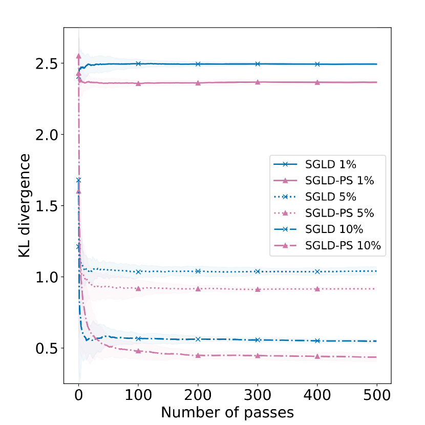
(a)

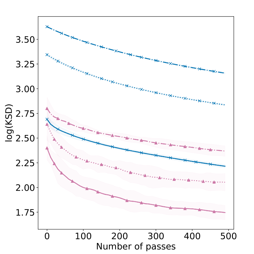
(b)

Figure 4: Sampler performance of SGLD and SGLD-PS for 1%, 5% and 10% subsample sizes over 500 passes through the data. (a) bivariate Gaussian model on synthetic data of size $N=10^{4}$ (y-axis: KL divergence); (b) logistic regression on the covertype data (y-axis: KSD).

F.2 Performance of adaptive subsampling

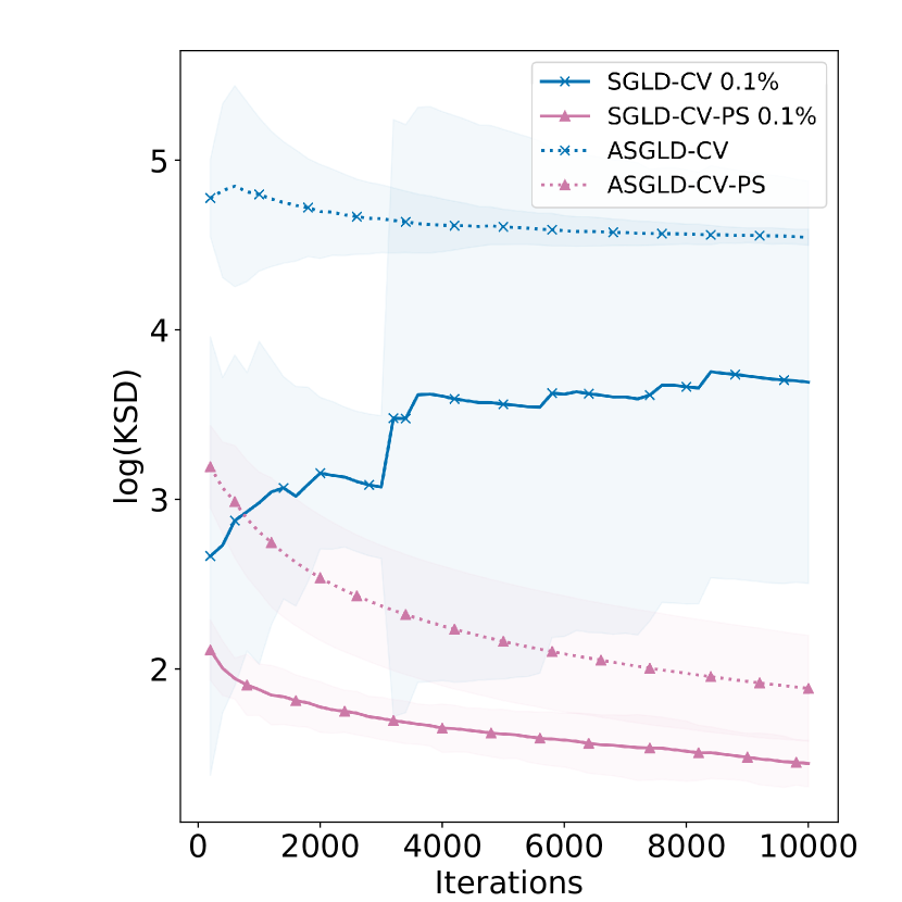
(a)

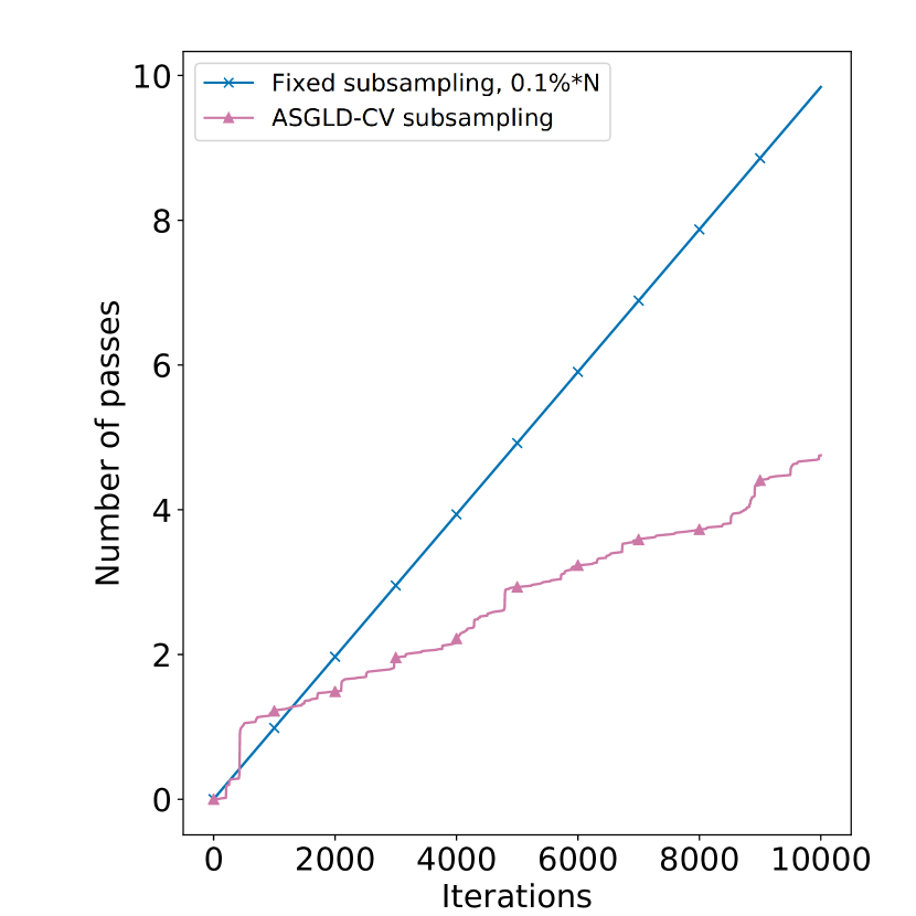
(b)

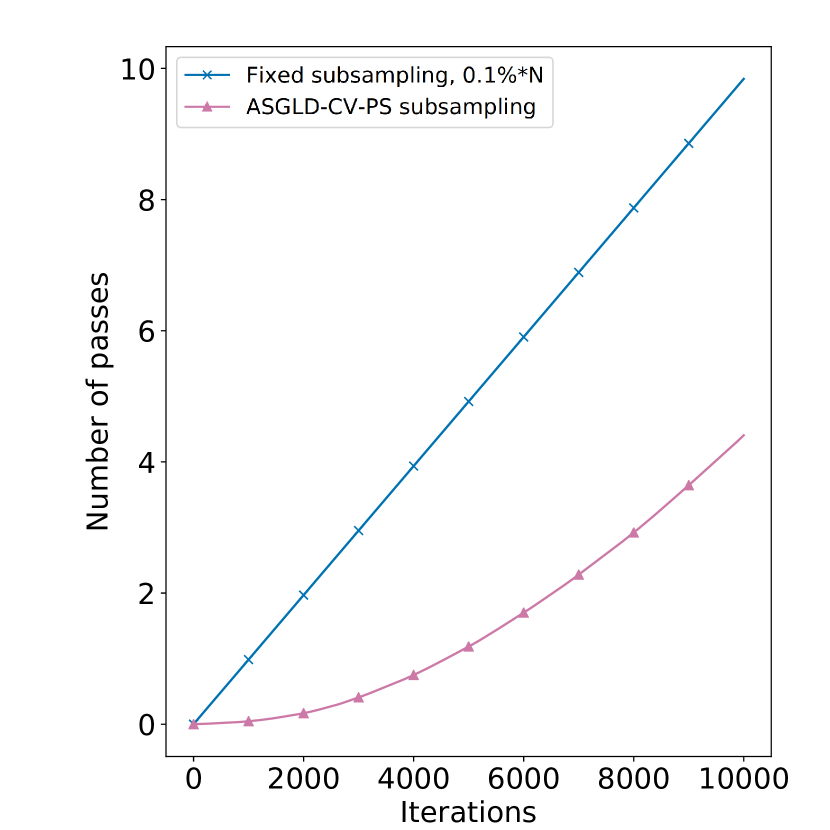
(c)

Figure 5: The linear regression model fitted on the CASP data. (a) KSD comparison of SGLD-CV, SGLD-CV-PS, ASGLD-CV and ASGLD-CV-PS over $10^{4}$ iterations; (b) the number of passes through the data achieved by fixed subsampling versus ASGLD-CV; (c) the number of passes through the data achieved by fixed subsampling versus ASGLD-CV-PS.

References

- Baker et al. (2019) Jack Baker, Paul Fearnhead, Emily B Fox, and Christopher Nemeth. Control variates for stochastic gradient MCMC. Statistics and Computing, 29(3):599–615, 2019.
- Blackard and Dean (1998) Jock A Blackard and Denis J Dean. Comparative Accuracies of Neural Networks and Discriminant Analysis in Predicting Forest Cover Types from Cartographic Variables. In Second Southern Forestry GIS Conference, pages 189–199, 1998.
- Bottou et al. (2018) Léon Bottou, Frank E Curtis, and Jorge Nocedal. Optimization Methods for Large-Scale Machine Learning. SIAM Review, 60(2):223–311, 2018.
- Chatterji et al. (2018) Niladri S Chatterji, Nicolas Flammarion, Yi-An Ma, Peter L Bartlett, and Michael I Jordan. On the Theory of Variance Reduction for Stochastic Gradient Monte Carlo. In Proceedings of the 35th International Conference on Machine Learning, volume 80 of Proceedings of Machine Learning Research, pages 764–773. PMLR, 10–15 Jul 2018.
- Chen et al. (2019) Changyou Chen, Wenlin Wang, Yizhe Zhang, Qinliang Su, and Lawrence Carin. A Convergence Analysis for A Class of Practical Variance-Reduction Stochastic Gradient MCMC. Science China Information Sciences, 62(12101), 2019.
- Chen et al. (2014) Tianqi Chen, Emily Fox, and Carlos Guestrin. Stochastic Gradient Hamiltonian Monte Carlo. In Proceedings of the 31st International Conference on Machine Learning, volume 32 of Proceedings of Machine Learning Research, pages 1683–1691. PMLR, 2014.
- Dalalyan and Karagulyan (2019) Arnak S. Dalalyan and Avetik Karagulyan. User-friendly guarantees for the Langevin Monte Carlo with inaccurate gradient. Stochastic Processes and their Applications, 129(12):5278–5311, 2019.
- Dubey et al. (2016) Kumar Avinava Dubey, Sashank J Reddi, Sinead A Williamson, Barnabas Poczos, Alexander J Smola, and Eric P Xing. Variance Reduction in Stochastic Gradient Langevin Dynamics. In Advances in Neural Information Processing Systems, volume 29, 2016.
- Durmus and Moulines (2019) Alain Durmus and Eric Moulines. High-dimensional Bayesian inference via the unadjusted Langevin algorithm. Bernoulli, 25(4A):2854–2882, 2019.
- Dwivedi et al. (2018) Raaz Dwivedi, Yuansi Chen, Martin J Wainwright, and Bin Yu. Log-concave sampling: Metropolis-Hastings algorithms are fast! In Proceedings of the 31st Conference On Learning Theory, volume 75 of Proceedings of Machine Learning Research, pages 793–797. PMLR, 2018.
- Fu and Zhang (2017) Tianfan Fu and Zhihua Zhang. CPSG-MCMC: Clustering-Based Preprocessing method for Stochastic Gradient MCMC. In Proceedings of the 20th International Conference on Artificial Intelligence and Statistics, volume 54 of Proceedings of Machine Learning Research, pages 841–850. PMLR, 2017.
- Gorham and Mackey (2017) Jackson Gorham and Lester Mackey. Measuring Sample Quality with Kernels. In Proceedings of the 34th International Conference on Machine Learning, volume 70 of Proceedings of Machine Learning Research, pages 1292–1301. PMLR, 2017.
- Hastings (1970) W.K. Hastings. Monte Carlo sampling methods using Markov chains and their applications. Biometrika, 57(1):97–109, 1970.
- Kern and Gyorgy (2016) Tamás Kern and A Gyorgy. SVRG++ with Non-uniform Sampling. In Proceedings of the 9th NIPS Workshop on Optimization for Machine Learning, 2016.
- Kingma and Ba (2016) Diederik P. Kingma and Jimmy Ba. Adam: A Method for Stochastic Optimization. In Proceedings of the 3rd International Conference on Learning Representations (ICLR), 2016.
- Li et al. (2021) Ruilin Li, Xin Wang, Hongyuan Zha, and Molei Tao. Improving Sampling Accuracy of Stochastic Gradient MCMC Methods via Non-uniform Subsampling of Gradients. Discrete and Continuous Dynamical Systems - S, 0, 2021.
- Liu et al. (2016) Qiang Liu, Jason Lee, and Michael Jordan. A Kernelized Stein Discrepancy for Goodness-of-fit Tests. In Proceedings of the 33rd International Conference on Machine Learning, volume 48 of Proceedings of Machine Learning Research, pages 276–284. PMLR, 2016.
- Liu et al. (2020) Rui Liu, Tianyi Wu, and Barzan Mozafari. Adam with Bandit Sampling for Deep Learning. In Advances in Neural Information Processing Systems, volume 33, pages 5393–5404, 2020.
- Metropolis et al. (1953) Nicholas Metropolis, Arianna W Rosenbluth, Marshall N Rosenbluth, Augusta H Teller, and Edward Teller. Equation of State Calculations by Fast Computing Machines. Journal of Chemical Physics, 21(6):1087–1092, 1953.
- Neal (2011) Radford M Neal. MCMC using Hamiltonian Dynamics. In Handbook of Markov Chain Monte Carlo, chapter 5. Chapman and Hall/CRC, 2011.
- Nemeth and Fearnhead (2021) Christopher Nemeth and Paul Fearnhead. Stochastic gradient Markov chain Monte Carlo. Journal of the American Statistical Association, 116(533):433–450, 2021.
- Parisi (1981) Giorgio Parisi. Correlation functions and computer simulations. Nuclear Physics B, 180(3):378–384, 1981.
- Robert and Casella (2004) Christian Robert and George Casella. Monte Carlo Statistical Methods. Springer Science & Business Media, 2nd edition, 2004.
- Roberts and Rosenthal (1998) Gareth O Roberts and Jeffrey S Rosenthal. Optimal scaling of discrete approximations to Langevin diffusions. Journal of the Royal Statistical Society: Series B (Statistical Methodology), 60(1):255–268, 1998.
- Roberts and Tweedie (1996) Gareth O Roberts and Richard L Tweedie. Exponential convergence of Langevin distributions and their discrete approximations. Bernoulli, pages 341–363, 1996.
- Salehi et al. (2017) Farnood Salehi, L Elisa Celis, and Patrick Thiran. Stochastic Optimization with Bandit Sampling. arXiv preprint arXiv:1708.02544, 2017.
- Schmidt et al. (2015) Mark Schmidt, Reza Babanezhad, Mohamed Ahmed, Aaron Defazio, Ann Clifton, and Anoop Sarkar. Non-Uniform Stochastic Average Gradient Method for Training Conditional Random Fields. In Proceedings of the Eighteenth International Conference on Artificial Intelligence and Statistics, volume 38 of Proceedings of Machine Learning Research, pages 819–828. PMLR, 2015.
- Schmidt et al. (2017) Mark Schmidt, Nicolas Le Roux, and Francis Bach. Minimizing Finite Sums with the Stochastic Average Gradient. Mathematical Programming, 162:83–112, 2017.
- Teh et al. (2016) Yee Whye Teh, Alexandre H Thiery, and Sebastian J Vollmer. Consistency and Fluctuations For Stochastic Gradient Langevin Dynamics. Journal of Machine Learning Research, 17(7):1–33, 2016.
- Vollmer et al. (2016) Sebastian J. Vollmer, Konstantinos C. Zygalakis, and Yee Whye Teh. Exploration of the (Non-)Asymptotic Bias and Variance of Stochastic Gradient Langevin Dynamics. Journal of Machine Learning Research, 17(159):1–48, 2016.
- Welling and Teh (2011) Max Welling and Yee Whye Teh. Bayesian Learning via Stochastic Gradient Langevin Dynamics. In Proceedings of the 28th International Conference on Machine Learning, pages 681–688, 2011.
- Zhang et al. (2017) Cheng Zhang, Hedvig Kjellstrom, and Stephan Mandt. Determinantal Point Processes for Mini-Batch Diversification. In Proceedings of the 33rd Conference on Uncertainty in Artificial Intelligence (UAI), pages 1–13, 2017.
- Zhao and Zhang (2014a) Peilin Zhao and Tong Zhang. Accelerating Minibatch Stochastic Gradient Descent using Stratified Sampling. arXiv preprint arXiv:1405.3080, 2014a.
- Zhao and Zhang (2014b) Peilin Zhao and Tong Zhang. Stochastic Optimization with Importance Sampling. arXiv preprint arXiv:1401.2753, 2014b.
- Zhao and Zhang (2015) Peilin Zhao and Tong Zhang. Stochastic Optimization with Importance Sampling for Regularized Loss Minimization. In Proceedings of the 32nd International Conference on Machine Learning, volume 37 of Proceedings of Machine Learning Research, pages 1–9. PMLR, 2015.