Deep Learning Object Detection Approaches to Signal Identification

Abstract

Traditionally Electromagnetic signal identification is using threshold-based energy detection algorithms. These algorithms frequently sum up the activity in regions, and consider regions above a specific activity threshold to be signal. While these algorithms work for the majority of cases, they often fail to detect signals that occupy small frequency bands, fail to distinguish signals with overlapping frequency bands, and cannot detect signals below a specified signal-to-noise ratio. Through the conversion of raw signal data to spectrogram, source identification can be framed as an object detection problem. By leveraging advancements in deep learning based object detection, we propose a system that manages to alleviate the failure cases encountered when using traditional source identification algorithms. Our contributions include framing signal identification as an object detection problem, the publication of a spectrogram object detection dataset, and evaluation of the RetinaNet and YOLOv5 object detection models trained on the dataset. Our models achieve Mean average Precisions (MaP) of up to 0.906. With such a high MaP, these models are sufficiently robust for use in real-world applications.

Index Terms—  Bounding box, YOLO, RetinaNet, Object Detection, deep dearning.

1 Introduction

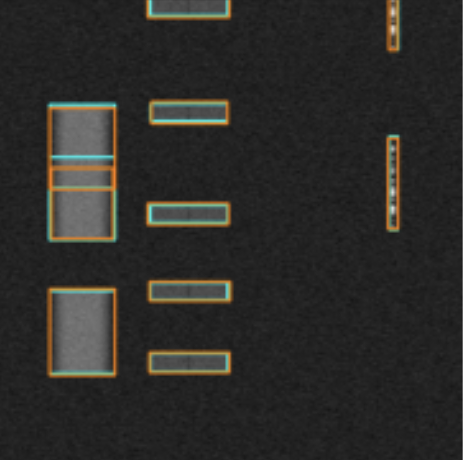
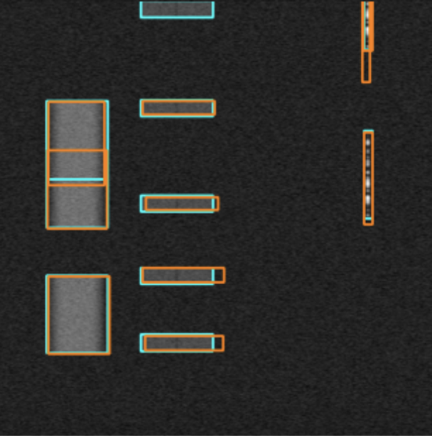
Fig. 1: A sampling of detections (orange box) and ground truths (cyan box) using the YOLOv5 (top) RetinaNet (bottom) model. Background spectrum grey-scale is normalized form 0-1. The frequency spans 100 MHz on the x-axis is and the time spans 50 ms on the y-axis. Notice the overlapping signals to the left.

Since the inception of YOLO[1], the object detection space has been dominated by deep learning based architectures. With the popularization of deep learning based object detection approaches, object detection models have become accuracy, robust and reliable.

By reframing signal identification as an object detection problem, we translate these advancements in deep learning based object detection to the signal detection problem. Our system tackle the failures cases of traditional activity-threshold based systems. These failure cases include failing to distinguish distinct signals, failure to detect signals occupying small frequency bands, and failure to detect signals below the signal to noise floor. One such case where traditional models fail is demonstrated in figure 1. In the left portion of the sample spectrogram multiple signals occupy a shared frequency space. This causes energy based detectors to identify them as a single signal. Our deep learning object detection approach to signal identification successfully distinguishes and detects both signals.

Alongside our publication we open source everything required to reproduce our results. This includes our annotated spectrogram dataset, training pipeline, and inference pipeline. Our final models include both YOLOv5 and RetinaNet models, capable of scoring 0.906 Mean Average Precision (MaP) on the dataset. Figure 1 shows nine frames annotated ground truth samples (blue) from the generated EM spectrum dataset along with detected bounding boxes (red). In a real-time system the frequency axis (x-axis) is 100 MHz and time axis (y-axis) is 50 ms each frame. Thus, we need to process 20 frames per second.

Our contributions include the framing of signal identification as an object detection problem, an object detection dataset consisting of spectrograms and bounding box annotations to accompany, a deep learning based signal identification system trained on the novel dataset, analysis of the distinctions between traditional object detection datasets and our dataset, and finally a comparison between our deep learning based approach and traditional energy based systems. The contributions can be broken into three components: problem framing, dataset production, and model training.

We present a novel object detection dataset as well as propose solutions to the dataset including a trained RetinaNet[2] and YOLOv5[3] architecture. YOLOv2 [4] and YOLOv3 has been used for EM spectrum detection obtaining 85% average prediction in their dataset [5].

Datasets of similar format include Common Objects in Context[6], Pascal VOC[7], and Kitti[8]. Our dataset differs primarily in the fact that instead of natural images, it consists of spectrogram images of EM signals.

Other object detection architectures that could be used to solve our dataset include Faster-RCNN [9], DINO SWIN-L[10], YoloX[11], and Yolov3[12].

We evaluate our models using MSCOCO metrics. These metrics were originally explained in the Common Objects in Context publication[6]. To evaluate our MSCOCO metrics we use both the pycocotools and KerasCV metric implementations [13].

While the COCO variant of Recall measures the models ability to detect all of the boxes in the validation set, the COCO variant of MaP incentivizes the detection of all boxes in the validation set while also punishing false positive. Mean Average Precision can be interpreted as a general purpose metric for the evaluation of an object detection model. More information on metric definitions and the process of their computation can be found in Ref. [14].

2 Data Generation

To demonstrate the effectiveness of our methodology, we present a synthetic dataset generated by Matlabs Communications Toolbox. Our dataset consists of 4686 annotated spectrogram samples. These samples contain a 512x512 image and 0-13 signals, each with a corresponding bounding box annotation.

The samples in the dataset consists of a spectrogram containing a variety of signals and annotations of the signal bounding boxes. All spectrograms were constructed from I/Q samples that were generated using the Matlab communications and signal processing toolboxes with a sampling rate of 100 MHz and a total transmission time of 50 ms. The signal types appearing in this dataset are direct-sequence spread spectrum (DSSS), Bluetooth low energy (BLE), quadrature amplitude modulation (QAM), amplitude modulation (AM), frequency modulation (FM), and WiFi with each sample having between one and four signals from this set. Signal metadata like center frequency, bandwidth, arrival time, and signal-to-noise ratio (SNR) are uniformly randomized between samples.

To generate samples for the dataset, a combination of signal types is first selected. Next, we initialize the signal and add white Gaussian noise. The center frequency, bandwidth, and SNR for each signal type are randomly selected, a signal generator is instantiated, and each signal is added to the source. After this signal metadata is configured, I/Q samples for 5 realizations of this configuration are generated with signal durations and arrival times being randomized between realizations.

We repeat this process of randomly selecting signal metadata and generating realizations 20 times for a given combination of signals, resulting in 100 total realizations of signal-level metadata for every combination. After all realizations are generated, the source is cleared, the I/Q samples and metadata are stored, and the entire process is repeated for a new combination of signals.

Spectrograms are constructed from the I/Q samples using a sampling rate of 100 MHz, 1024 discrete Fourier transforms, an overlap length of 128 samples. The spectrograms are resized to 512x512 with bicubic interpolation and saved as PNG images. The coordinates for the bounding box annotations for the signals in an image are calculated from the signal metadata and saved in a corresponding text file. These images and labels are the dataset used in training the models.

2.1 Difficulties of Spectogram Object Detection

In our initial experiment, we train a RetinaNet with the library default settings for the RetinaNet. This includes the default settings for IoU threshold for label encoding, IoU threshold for label decoding, and the default configuration for the AnchorBox generation process.

In initial experiments, the loss converged to low values on both the training and validation sets. Despite this, the model only achieves an MaP of 0.205 and a Recall of 0.238 . These are intolerable results for use in a production system.

The reason that the loss converges to such a low loss but the MaP and Recall remain low stems from the regular shapes of objects in the EM spectrograms. While most objects in the natural world follow a smooth distribution for aspect ratio spectrograms have no such property. This leads the signals present in the spectrograms to have a wide array of aspect ratios. As such, the anchor boxes generated by the default configuration used in the KerasCV RetinaNet are unlikely to match with the boxes from our training dataset in the label encoding process. This leads to the boxes that are not encoded having no representation in the encoded batch of encoded training targets. This explains the low loss, low Recall, and low MaP.

The reason that anchor configuration is particularly important for spectrogram object detection is attributed to the wide, distribution of aspect ratios and side lengths of the spatial representations of the bounding box annotations. This is shown in a histograms in figures 2 and 3.

This differs greatly from object annotations present in natural images. For comparison, the aspect ratio and side length distributions for PascalVOC can be seen in figures 2 and 3.

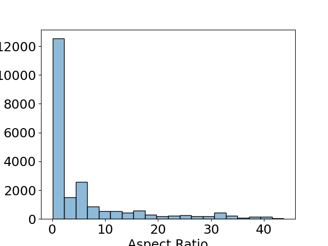
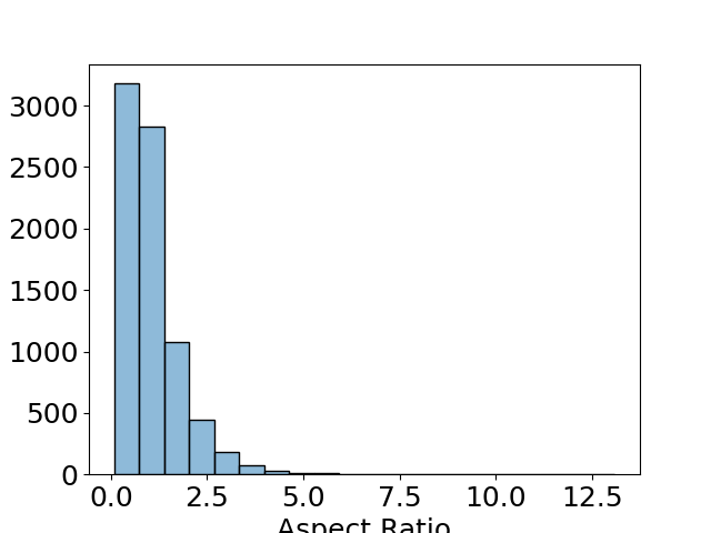
Fig. 2: Aspect ratio histogram of spectrograms (left) and PascalVOC objects (right).

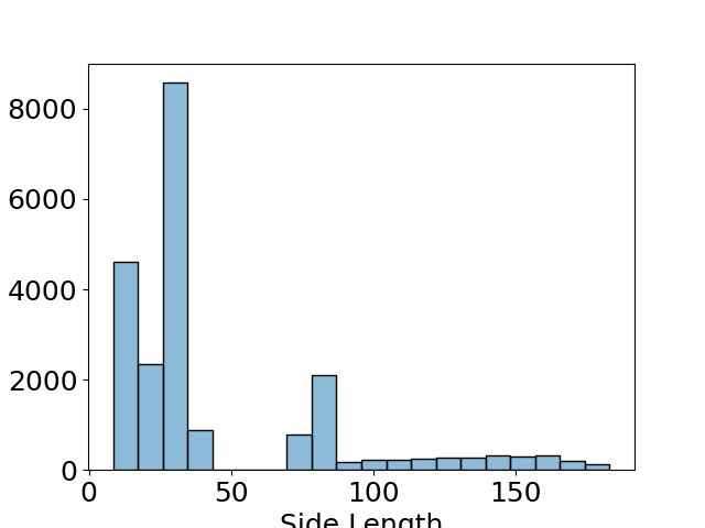
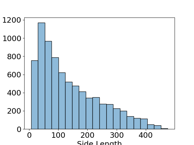
Fig. 3: Side length in pixels histogram of spectrograms (left) and. PascalVOC objects (right).

3 Training & Experimental Results

Using the dataset produced using the process described in section 2, we can train any deep learning based object detection model. Our models are trained on a pre-generated train test split. This split consists of 3859 training images, and 827 test images. The object detection models are evaluated based on two metrics: the standard variant of MaP and Recall used in the MSCOCO challenge. We leverage the KerasCV COCO metric, and parameterize them as described in [14]. Using these implementations enables to perform train time evaluation of these metrics.

Due to the high cost of computation required to compute MaP we do not evaluate the true MaP during training. Instead, the approximate COCO metrics is obtained by evaluating for a subset of 20 images from the evaluation dataset define. Using this proxy, we evaluate our model’s performance across epochs and monitor its train time progress. Final metrics are evaluated on the entirety of the test set. As an additional inference test, we manually examine the visual results of the predictions.

3.1 RetinaNet

In the first experiment, RetinaNet is trained using the KerasCV[13] library. The RetinaNet[2] architecture uses a ResNet50[15] backbone, which achieve about 30 frames per second on a standard consumer GPU. With a MobileNetv3[16] backbone, a RetinaNet can achieve up to 60 FPS on a consumer GPU, enabling real time signal identification. We configure the aspect ratios for the anchor box generator according to the results of section 2.1. We do not configure the anchor generator according to the side lengths. This results in the model not detecting the small boxes.

During training, spectrograms are loaded into memory as tensors of shape $(512,512,3)$ with pixel values in the range of $[0,255]$. Pixel values are rescaled to the range $[0,1]$ by dividing by 255.

The backbone used is a ResNet50, with weights initialized using the weights produced by training a ResNet50 to perform image classification. Our feature pyramid, prediction heads, and backbone are all trained using the spectogram dataset. A SGD optimizer with a global clip norm[17] of $10.0$ is used for fitting, with a batch size 8. Without the global clip norm, the loss explodes due to steep gradients existing at many points in the loss landscape. Training is lightweight; ours being performed on a single GPU A100. The learning rate of our optimizer is reduced after 5 epochs of training with no loss improvement on the validation set, and training stops once no improvement has been seen in 20 epochs.

No data augmentation was used to train the RetinaNet model as it decreased performance. This is due to that spectrograms have different bounding box distribution than natural images. As such, traditional augmentation techniques such as RandomFlip, RandomShear, and others are not useful.

Losses alongside MaP and Recall metrics are shown in figures 4. Results for all metrics are in Table 1. Upon convergence the RetinaNet model achieves a Recall of 0.565 and MaP of 0.492 .

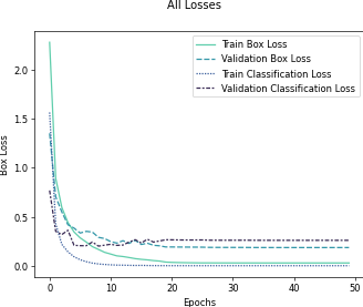
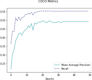
Fig. 4: Losses (left) and COCO metrics (right) for the RetinaNet model

3.2 YOLOv5

To test the usefulness of various augmentation schemes and superior anchor configuration, we train a model using the pre-configured YOLOv5 framework maintained by Ultralytics[3]. The YOLOv5s architecture consists of a CSPDarknet53, a PANet feature pyramid, and a YOLOv4 head to generate the final output vectors with bounding boxes, class probabilities, and objectness scores. The Ultralytics YOLOv5 framework automatically tunes anchor boxes for aspect ratio and side length, and includes the Mosaic augmentation[3] technique. The mosaic augmentation is a logical choice for spectrogram object detection as due to the spatial meaning embedded in spectrograms translations, rotations, and color based augmentations all become meaningless.

A for RetinaNet, spectrograms are loaded into memory as tensors of shape (512,512,3) with normalized pixel values in the range [0,1]. A standard Keras stochastic gradient descent optimizer is used with a batch size of 16 and a warmup scheduler with a relatively low learning rate for 3 epochs as it ramps up to the normal learning rate. Training is done on a single NVIDIA T4 GPU over 50 epochs and set to stop once no improvement has been seen in 20 epochs.

The loss function for YOLOv5 is a summation of a box loss, objectness loss, and classification loss. The classification loss is here ignored as there is only one class. Losses and COCO metrics are shown in Figure 5. The YOLOv5s model achieves much better Recall and MaP than RetinaNet.

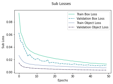
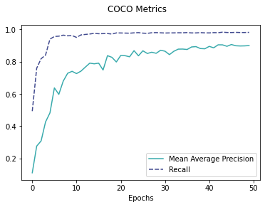
Fig. 5: Losses (left) and COCO metrics (right) for the YOLOv5 Model

3.3 Experimental Analysis

Our experiments show that a deep learning based approach to signal identification is highly robust, the importance of anchor configuration in spectrogram object detection, and the effectiveness of the Mosaic data augmentation. In training our RetinaNet, we initially did not tune the anchor generator at all. This yielded incredibly poor results, with a final MaP of 0.2. Upon configuring only the aspect ratios, we scored an MaP of 0.492. Finally, we train a YOLOv5 model with optimal anchor configuration and achieve a MaP of 0.906.

In addition to the optimal anchor configuration, we determine that the mosaic augmentation significantly boosts performance. This is a reasonable result; given that most other data augmentation techniques are no longer applicable in the spectral domain. For example, rotations, color jitter, and many other common augmentations are no longer suitable when working with spectrograms. Mosaic, on the other hand maintains the spatial structure of most the signals while still producing synthetic data. Our two best models scores are available in table 1.

	MaP	Recall
YOLOv5	0.906	0.980
RetinaNet	0.492	0.565

Table 1: Metrics for both the YOLOv5 and RetinaNet models.

4 Conclusion

Through reframing of signal identification as an object detection problem we leverage advancements in deep learning based object detection to handle the failure cases of traditional signal identification systems. These failure cases include failing to distinguish distinct signals, failure to detect signals occupying small frequency bands, and failure to detect signals below the signal to noise floor.

We presented and open source a dataset consisting of 7000 spectrograms alongside bounding box annotations annotations of the signals present in these spectrograms, an open source Python library to load the dataset into a TensorFlow dataset, an open source training script to train a KerasCV RetinaNet on our novel dataset, and a sample solution to the dataset using YOLOv5. We analyzed the data to produce optimal anchor box configuration for deep learning based object detection systems. This show the distinct importance of anchor configuration in spectrogram object detection.

The YOLOv5 model achieved a Mean average Precision (MaP) of 0.906 and Recall of 0.980. These metrics indicate that the model detects almost all signals boxes while making minimal false positive predictions. Our model is sufficiently robust for deployment in a real world system.

References

- [1] Joseph Redmon, Santosh Divvala, Ross Girshick, and Ali Farhadi, “You only look once: Unified, real-time object detection,” 2015.
- [2] Tsung-Yi Lin, Priya Goyal, Ross Girshick, Kaiming He, and Piotr Dollár, “Focal loss for dense object detection,” in Proceedings of the IEEE international conference on computer vision, 2017, pp. 2980–2988.
- [3] Glenn Jocher et al., “ultralytics/yolov5: v6.2 - YOLOv5 Classification Models, Apple M1, Reproducibility, ClearML and Deci.ai integrations,” Aug. 2022.
- [4] Tim O’Shea, Tamohgna Roy, and T Charles Clancy, “Learning robust general radio signal detection using computer vision methods,” in 2017 51st asilomar conference on signals, systems, and computers. IEEE, 2017, pp. 829–832.
- [5] Adela Vagollari, Viktoria Schram, Wayan Wicke, Martin Hirschbeck, and Wolfgang Gerstacker, “Joint detection and classification of rf signals using deep learning,” in 2021 IEEE 93rd Vehicular Technology Conference (VTC2021-Spring). IEEE, 2021, pp. 1–7.
- [6] Tsung-Yi Lin, Michael Maire, Serge Belongie, James Hays, Pietro Perona, Deva Ramanan, Piotr Dollár, and C Lawrence Zitnick, “Microsoft coco: Common objects in context,” in European conference on computer vision. Springer, 2014, pp. 740–755.
- [7] Mark Everingham, Luc Van Gool, Christopher KI Williams, John Winn, and Andrew Zisserman, “The pascal visual object classes (voc) challenge,” International journal of computer vision, vol. 88, no. 2, pp. 303–338, 2010.
- [8] Andreas Geiger, Philip Lenz, and Raquel Urtasun, “Are we ready for autonomous driving? the kitti vision benchmark suite,” in 2012 IEEE conference on computer vision and pattern recognition. IEEE, 2012, pp. 3354–3361.
- [9] Shaoqing Ren, Kaiming He, Ross Girshick, and Jian Sun, “Faster r-cnn: Towards real-time object detection with region proposal networks,” Advances in neural information processing systems, vol. 28, 2015.
- [10] Ze Liu, Yutong Lin, Yue Cao, Han Hu, Yixuan Wei, Zheng Zhang, Stephen Lin, and Baining Guo, “Swin transformer: Hierarchical vision transformer using shifted windows,” in Proceedings of the IEEE/CVF International Conference on Computer Vision, 2021, pp. 10012–10022.
- [11] Zheng Ge, Songtao Liu, Feng Wang, Zeming Li, and Jian Sun, “Yolox: Exceeding yolo series in 2021,” arXiv preprint arXiv:2107.08430, 2021.
- [12] Joseph Redmon and Ali Farhadi, “Yolov3: An incremental improvement,” arXiv preprint arXiv:1804.02767, 2018.
- [13] Luke Wood, Scott Zhu, François Chollet, et al., “Keras cv,” https://github.com/keras-team/keras-cv, 2022.
- [14] Luke Wood and Francois Chollet, “Efficient graph-friendly coco metric computation for train-time model evaluation,” 2022.
- [15] Kaiming He, Xiangyu Zhang, Shaoqing Ren, and Jian Sun, “Identity mappings in deep residual networks,” 2016.
- [16] Andrew Howard, Mark Sandler, Grace Chu, Liang-Chieh Chen, Bo Chen, Mingxing Tan, Weijun Wang, Yukun Zhu, Ruoming Pang, Vijay Vasudevan, Quoc V. Le, and Hartwig Adam, “Searching for mobilenetv3,” 2019.
- [17] Jingzhao Zhang, Tianxing He, Suvrit Sra, and Ali Jadbabaie, “Why gradient clipping accelerates training: A theoretical justification for adaptivity,” 2019.