Abstract

Recent work on the Lottery Ticket Hypothesis (LTH) shows that there exist “winning tickets” in large neural networks. These tickets represent “sparse” versions of the full model that can be trained independently to achieve comparable accuracy with respect to the full model. However, finding the winning tickets requires one to pretrain the large model for at least a number of epochs, which can be a burdensome task, especially when the original neural network gets larger.

In this paper, we explore how one can efficiently identify the emergence of such winning tickets, and use this observation to design efficient pretraining algorithms. For clarity of exposition, our focus is on convolutional neural networks (CNNs). To identify good filters, we propose a novel filter distance metric that well-represents the model convergence. As our theory dictates, our filter analysis behaves consistently with recent findings of neural network learning dynamics. Motivated by these observations, we present the LOttery ticket through Filter-wise Training algorithm, dubbed as LoFT. LoFT is a model-parallel pretraining algorithm that partitions convolutional layers by filters to train them independently in a distributed setting, resulting in reduced memory and communication costs during pretraining. Experiments show that LoFT $i)$ preserves and finds good lottery tickets, while $ii)$ it achieves non-trivial computation and communication savings, and maintains comparable or even better accuracy than other pretraining methods.

1 Introduction

The Lottery Ticket Hypothesis (LTH) Frankle and Carbin, (2018) claims that neural networks (NNs) contain subnetworks (“winning tickets”) that can match the dense network’s performance when fine-tuned in isolation. Yet, identifying such subnetworks often requires proper pretraining of the dense network. Empirical studies based on this statement show that NNs could potentially be significantly smaller without sacrificing accuracy Chen et al., (2020); Frankle et al., (2019); Gale et al., (2019); Liu et al., (2018); Morcos et al., (2019); Zhou et al., (2019); Zhu and Gupta, (2017). How to efficiently find such subnetworks remains a widely open question: since LTH relies on a pretraining phase, it is a de facto criticism that finding such pretrained models could be a burdensome task, especially when one focuses on large NNs.

This burden has been eased with efficient training methodologies, which are often intertwined with pruning steps. Simply put, one has to answer two fundamental questions: “When to prune?” and “How to pretrain such large models?”.  Focusing on “When to prune?”, one can prune before Lee et al., (2018, 2019); Wang et al., 2019b , after LeCun et al., (1990); Hassibi et al., (1993); Dong et al., (2017); Han et al., 2015b ; Li et al., (2016); Molchanov et al., (2019); Han et al., 2015a ; Wang et al., 2019a ; Zeng and Urtasun, (2019), and/or during pretraining Frankle and Carbin, (2018); Srinivas and Babu, (2016); Louizos et al., (2018); Bellec et al., (2018); Dettmers and Zettlemoyer, (2019); Mostafa and Wang, (2019); Mocanu et al., (2018). Works like SNIP Lee et al., (2018, 2019) and GraSP Wang et al., 2019b aim to prune without pretraining, while suffering some accuracy loss. Pruning after training often leads to favorable accuracy, with the expense of fully training a large model. A compromise between the two approaches exist in early bird tickets You et al., (2019), where one could potentially avoid the full pretraining cost, but still identify “winning tickets”, by performing a smaller number of training epochs and lowering the precision of computations. This suggests the design of more efficient pretraining algorithms that target specifically at identifying the winning tickets for larger models.

Focusing on “How to pretrain large models?”, modern large-scale neural networks come with significant computational and memory costs. Researchers often turn to distributed training methods, such as data parallel and model parallel Zinkevich et al., (2010); Agarwal and Duchi, (2011); Stich, (2019); Ben-Nun and Hoefler, (2018); Zhu et al., (2020); Gholami et al., (2017); Guan et al., (2019); Chen et al., (2018), to enable heavy pretraining towards finding winning tickets, by using clusters of compute nodes. Yet, data parallelism needs to update the whole model on each worker—which still results in a large memory and computational cost. To handle such cases, researchers utilize model parallelism, such as Gpipe Huang et al., (2019), to reduce the per node computational burden. Traditional model parallelism enjoys similar convergence behaviour as centralized training, but needs to synchronize at every training iteration to exchange intermediate activations and gradient information between workers, thus often incurring high communication cost.

Our approach and contributions. We propose a new model-parallel pretraining method on the one-shot pruning setting that can efficiently reveal winning tickets for CNNs. In particular, we center on the following questions:

“What is a characteristic of a good pretrained CNN that contains the winning ticket? How will such a criterion inform our design towards efficient pretraining?”

Prior works show that filter-wise pruning is more preferable compared to weight pruning for CNNs Huang et al., (2019); He et al., (2020); da Cunha et al., (2022); Wang et al., (2021); Li et al., (2016). Our approach operates by decomposing the full network into narrow subnetworks via filter-wise partition during pretraining. These subnetworks –which are randomly recreated intermittently during the pretraining process– are trained independently, and their updates are periodically aggregated into the global model. Because each subnetwork is much smaller than the full model, our approach enables scaling beyond the memory limit of a single GPU. Our methodology allows the discovery of winning tickets with less memory and a lower communication budget. The contributions are summarized as follows:

• We propose a metric to quantify the distance between tickets in different stages of pretraining, allowing us to characterize the convergence to winning tickets throughout the pretraining process.

• We identify that such convergence behavior suggests an alternative way of pretraining: we propose a novel model-parallel pretraining method through filter-wise partition of CNNs and iterative training of such subnetworks.

• We theoretically show that our proposed method achieves CNN weight that is close to the weight found by gradient descent in a simplified scenario.

• We empirically show that our method provides a better or comparable winning ticket, while being memory and communication efficient.

2 Preliminaries

The CNN model He et al., (2015); Krizhevsky et al., (2012); Simonyan and Zisserman, (2015) is composed of convolutional layers, batch norm layers Ioffe and Szegedy, (2015), pooling layers, and a final linear classifier layer. Our goal is to retrieve a structured winning ticket, through partitioning and pruning the filters in the convolutional layers.

Mathematically, we formulate this process as follows. Let $p_{i}$ denote the number of input channels for the $i$-th convolutional layer. Correspondingly, the output channel of the $i$-th layer is the same as the input channel of the $(i+1)$-th layer, which is $p_{i+1}$. Let $h_{i}$,$w_{i}$ be the height and width of the input feature maps, respectively. Then, the $i$-th convolutional layer transforms the input feature map $x_{i}\in\mathbb{R}^{p_{i}\times h_{i}\times w_{i}}$ into the output feature map $x_{i+1}\in\mathbb{R}^{p_{i+1}\times h_{i+1}\times w_{i+1}}$ by performing 2D convolutions on the input feature map with $p_{i+1}$ filters of size $3\times 3$, where the $j$-th filter is denoted as $\mathcal{F}_{i,j}\in\mathbb{R}^{p_{i}\times 3\times 3}$. Thus the total filter weight for the $i$-th layer is $\mathcal{F}_{i}\in\mathbb{R}^{p_{i+1}\times p_{i}\times 3\times 3}$. Formally, prunning $\nicefrac{{1}}{{k}}$ of the filters in the $i$-th layer is equivalent to discarding $\nicefrac{{p_{i+1}}}{{k}}$ filters. Thus the resulted total pruned filter weight is in $\mathbb{R}^{\nicefrac{{p_{i+1}\cdot(k-1)}}{{k}}\times p_{i}\times 3\times 3}$ and the output feature map $x_{i+1}$ is in $\mathbb{R}^{\nicefrac{{p_{i+1}\cdot(k-1)}}{{k}}\times h_{i+1}\times w_{i+1}}$.

3 Identifying Tickets Early in Training

In this section, we aim at answering the following questions to motivate the design of an efficient pretraining algorithm:

“How do we compare different winning filters? How early can we observe winning filters?”

3.1 Evaluate the distance of two pretrained models

With the goal of identifying tickets early in training, we study when we can prune to find a winning ticket reliably, which oftentimes occurs before training accuracy stabilizes You et al., (2019). Thus, we need a metric to evaluate how trained filters evolve towards being stabilized, as the iterations increase and before they get pruned. Since at pruning time we care about the relative magnitude of the filter weights, this question can be abstracted as finding the distance of two different rankings of a given set of filters.

Borrowing techniques from search system rankings Kumar and Vassilvitskii, (2010), we propose a filter distance metric based on a position-weighted version of Spearman’s footrule Spearman, (1987). In particular, consider evaluating the distance between trained convolutional layers at epochs $X$ and $Y$. Denote their the filters at epochs $t_{1}$ and $t_{2}$ on the $i$-th layer as $\mathcal{F}^{(t_{1})}_{i},\mathcal{F}^{(t_{2})}_{i}$. We calculate the $\ell_{2}$-norm of $\mathcal{F}^{(t_{1})}_{i,j},\mathcal{F}^{(t_{2})}_{i,j}$ for each filter index $j\in[p_{i+1}]$ and sort them by magnitude. We denote the two sorted list with length $p_{i+1}$ as $R^{(t_{1})}$ and $R^{(t_{2})}$. Each of these lists contains the $\ell_{2}$-norm of the filters, namely $\left\|\mathcal{F}^{(t_{1})}_{i,j}\right\|_{2}$ and $\left\|\mathcal{F}^{(t_{2})}_{i,j}\right\|_{2}$.

We represent the change in ranking from $R^{(t_{1})}$ to $R^{(t_{2})}$ as $\sigma$. I.e., if $x\in R^{(t_{1})}$ is the $i$-th element in $R^{(t_{1})}$, then, the ranking of $x$ in $R^{(t_{2})}$ is denoted as $\sigma(i)$. The original Spearman’s footrule defines the displacement of element $i$ as $|i-\sigma(i)|$, leading to the total displacement of all elements:

$$F(\sigma)=\sum_{i}|i-\sigma(i)|.$$

Given weights $w_{i}$’s for the elements, the weighted displacement for element $i$ becomes $w_{i}\cdot\left|\sum_{j<i}w_{j}-\sum_{\sigma(j)<\sigma(i)}w_{j}\right|$, leading to the total weighted displacement as follows:

$$F_{w}(\sigma)=\sum_{i}w_{i}\cdot\left(\left|\sum_{j<i}w_{j}-\sum_{\sigma(j)<\sigma(i)}w_{j}\right|\right).$$

To put emphasis on the correct ranking of the top elements, we set the position weight for the $i$-th ranking element as $1/i$. To further simplify calculations, we approximate $\sum_{i=1}^{n}\frac{1}{i}\approx\ln(n)-\ln(1)$ where $\ln(\cdot)$ is the natural logarithm. The above lead to the following definition for our filter distance:

$$F_{\text{filter}}(\sigma)=\sum_{i}\tfrac{1}{i}\cdot\left|\ln(i)-\ln(\sigma(i))\right|.$$

For the case where the two lists of pruned filters do not contain the same elements, we can naturally define the distance when the $i$-th element is not in the other list to be $|\ln(l+1)-\ln(i)|$; $l$ is the length of the pruned filter list. This filter distance metric is fundamentally different from the mask distance proposed in You et al., (2019). A detailed comparison can be found in Related Work. We compare against these early-pruning methods in the experiments.

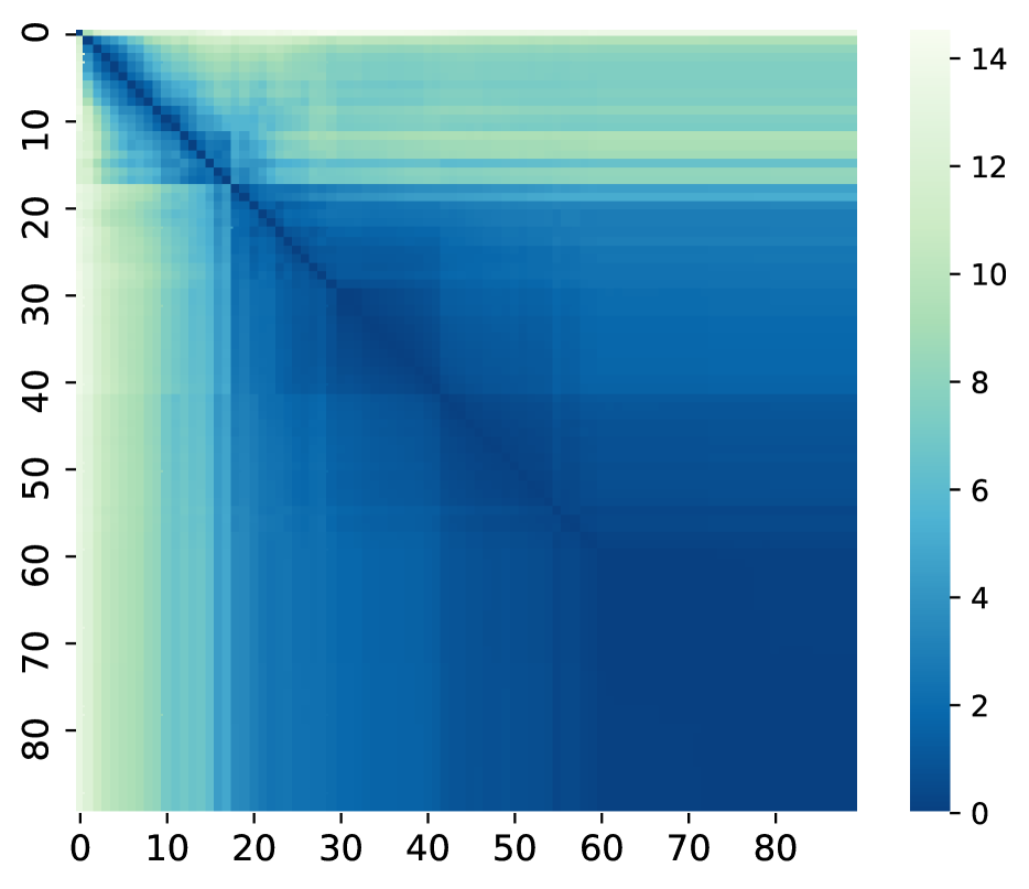
(a) conv-layer2

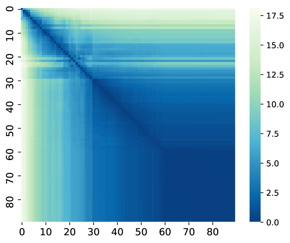
(b) conv-layer3

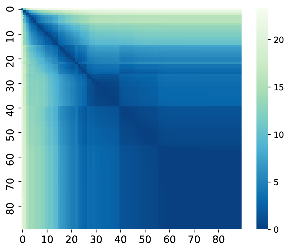
(c) conv-layer4

Figure 1: Heatmap visualization of the pairwise mask distance for different layers of WideResNet18 trained on ImageNet. The $(i,j)$-th matrix element denotes the filter distance of a given filter between the $i$-th and $j$-th iteration. Lighter color indicates a larger filter distance, while a smaller filter distance is depicted with a darker blue color.

3.2 How early can we observe winning filters?

With the filter distance defined, we first visualize its behavior over a CNN as a function of training epochs. Figure 1 plots the pairwise filter distance of a WideResNet18 network Zagoruyko and Komodakis, (2016) on the ImageNet dataset Deng et al., (2009). Here, the $(i,j)$-th element in the heatmaps denotes the filter distance of a given filter in the network, between the $i$-th and $j$-th iteration in the experiment. Lighter coloring indicates a larger filter distance, while a smaller filter distance is depicted with a darker color.

Across all layers, during the first $\sim$ 15 epochs, the filter distance is changing rapidly between training epochs, as is indicated by the rapidly shifting color beyond the diagonal. Between $\sim$ 15 to $\sim$ 60 epochs, filter ranking has relatively converged as the model is learning to fine-tune its weights. Finally, at around the $\sim$ 60-th epoch, the filter distance becomes fully stable and we can observe a solid blue block at the lower right corner. This observation provides intuition that concur the hypothesis in Achille et al., (2019) about a critical learning period, and observation by You et al., (2019) using mask-distance on Batch Normalization (BN) layers.

3.3 Rethinking the Property of Winning Tickets

The empirical analysis above suggests that training the CNN weights until loss converges is not necessary for the discovery of winning tickets. However, many existing pretraining algorithms do not exclude heavy training over the whole CNN model. Even though one could utilize distributed solutions with multiple workers (like the data parallel and model parallel protocols), these come with uncut computation, memory and communication costs, since these algorithms are originally designed for training to convergence. These facts demand a new pretraining algorithm, targeting specifically at efficiently finding winning tickets.

Knowing the winning filters beforehand would greatly reduce the pretraining cost, but this is hard to achieve in practice. As a compromise, we can turn to the following question: “ Can we randomly sample “tickets” during pretraining, and independently train them in parallel on different workers, with the hope to preserve the winning tickets?” This would enable a highly efficient distributed implementation: subsets of tickets can be trained independently on each worker, with limited communication cost and less computational cost per worker.

To reduce the total computation and memory cost, one could only consider a small number of disjoint tickets per distributed worker. Yet, this simple heuristic should be used cautiously: in particular, splitting only once the convolutional filters –with no further communication between workers– could miss the global winning ticket, since no interaction is assumed between “locally” trained filters, leading to a strong greedy solution. This suggests that, in order to recover a good ticket, one needs to sample and train sufficiently large number of tickets to (heuristically) assure that “a good portion” of filters is trained, as well as different combinations of filters are tested in each iteration.

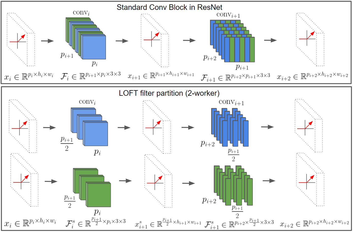
Figure 2: Depiction of the effect of a filter-wise LoFT partition on parameter sizes. Dotted blocks represent feature maps, colored blocks represent filters within convolutional layers.

This motivates our approach: we propose sampling and training different sets of tickets during different stages of the pretraining. In this way, the algorithm is expected to “touch” upon the potential winning tickets at certain iterations. We conjecture (this is empirically shown in our experiments) that important filters in such winning tickets can be preserved and further recovered at the end of pretraining using our approach. These observations led us to the definition of the LoFT algorithm.

4 The LoFT Algorithm

Algorithm 1 LoFT Algorithm

1:  Parameter: $T$ synchronization iterations in pretraining, $S$ workers, $\ell$ local iterations, $W$ CNN weights,

2:  $h(W)$ $\leftarrow$ randomly initialized CNN.

3:  for $t=0,\dots,T-1$ do

4:     $\left\{h_{s}(W_{s})\right\}_{s=1}^{S}={\color[rgb]{0,.5,.5}\text{{filterPartition}}}(h(W),~{}S)$

5:     Distribute each $h_{s}(W_{s})$ to a different worker.

6:     for $s=1,\dots,S$ do

7:        Train $h_{s}(W_{s})$ for $\ell$ iterations using local SGD.

8:     end for

9:     $h(W)={\color[rgb]{.5,0,.5}\texttt{aggregate}}\left(\left\{h_{s}(W_{s})\right\}_{s=1}^{S}\right)$.

10:  end for

We treat “sampling and training sets of tickets” as a filter-wise decomposition of a given CNN, where each ticket is a subnetwork with a subset of filters. This is shown in Fig. 2. The LoFT algorithm that implements our ideas is shown in Algorithm 1. Each block within a CNN typically consists of two identical convolutional layers, $\text{conv}_{i}$ and $\text{conv}_{i+1}$. As shown in Figure 2, our methodology operates by partitioning the filters of these layers, $\mathcal{F}_{i}$ and $\mathcal{F}_{i+1}$, to different subnetworks –see filterPartition() step in Algorithm 1– in a structured, disjoint manner. These subnetworks are trained independently –see local SGD steps in Algorithm 1– before aggregating their updates into the global model by directly placing the filters back to their original place—see aggreegate() step in Algorithm 1. The full CNN is never trained directly.

The filter-wise partition strategy for a convolutional block begins by disjointly partitioning the filters $\mathcal{F}_{i}$ of the first convolutional layer $\text{conv}_{i}$. This operation can be implemented by permuting and chunking the indices of filters within the first convolutional layer and within the block, as shown in Figure 2. Formally, we randomly and disjointly partition the total $p_{i+1}$ filters into $S$ subsets, where each subset forms $\mathcal{F}_{i}^{s}\in\mathbb{R}^{(p_{i+1}/S)\times p_{i}\times 3\times 3}$. $S$ here indicates the number of independent workers in the distributed system. $\mathcal{F}_{i}^{s}$ forms a new convolutional layer, which produces a new feature map $x_{i+1}^{s}\in\mathbb{R}^{(p_{i+1}/S)\times h_{i+1}\times w_{i+1}}$ with $S$ times fewer channels.

Based on which channels are presented in the feature map $x_{i+1}^{s}$, we further partition the input channels of filters $\mathcal{F}_{i+1}$ in the second convolutional layer into $S$ sets of sub-filters (Figure 2). Formally, each set has $p_{i+2}$ sub-filters with $\nicefrac{{p_{i+1}}}{{S}}$ input channels, $\mathcal{F}_{i+1}^{s}\in\mathbb{R}^{p_{i+2}\times\nicefrac{{p_{i+1}}}{{S}}\times 3\times 3}$ and produces a new feature map $x_{i+2}^{s}\in\mathbb{R}^{p_{i+2}\times h_{i+2}\times w_{i+2}}$. The input/output dimensions of the convolutional block are unchanged. We repeat the partition for all convolutional blocks in a CNN to get a set of subnetworks with disjoint filters. In each subnetwork, the intermediate dimensions of activations and filters are reduced, resembling a “bottleneck” structure.

Our methodology of choosing tickets/subnetworks avoids partitioning layers that are known to be most sensitive to pruning, such as strided convolutional blocks Liu et al., (2018). Parameters not partitioned are shared among subnetworks, so their values must be averaged when the updates of tickets/subnetworks are aggregated into the global model.

Compared with common distributed protocols, our pretraining methodology $i)$ reduces the communication costs, since we only communicate the tickets/subnetworks; and $ii)$ reduces the computational and memory costs on each worker, since we only locally train the sampled tickets/subnetworks that are smaller than the global model. From a different pespective, our approach allows pretraining networks beyond the capacity of a single-GPU: The global model could be a factor of $O(S)$ wider than each subnetwork, allowing the global model size to be extended far beyond the capacity of single GPU. The ability to train such “ultra-wide” models is quite promising for pruning purposes.

After pretraining with LoFT. We perform standard pruning on the whole network to recover the winning ticket, and use standard training techniques over this winning ticket until the end of training.

5 Theoretical Result

We perform theoretical analysis on a one-hidden-layer CNN (see figure 3), and show that the trajectory of the neural network weight in LoFT stays near to the trajectory of gradient descent (GD). Since filter pruning is based on magnitude ranking of the filters, a small difference between the filters learned with LoFT and the filters learned with GD will more likely preserve the winning tickets.

Consider a training dataset $(\mathbf{X},\mathbf{y})=\{(\mathbf{x}_{i},y_{i})\}_{i=1}^{n}$, where each $\mathbf{x}_{i}\in\mathbb{R}^{\hat{d}\times p}$ is an image and $y_{i}$ being its label. Here, $\hat{d}$ is the number of input channels and $p$ the number of pixels. Let $q$ denote the size of the filter, and let $m$ be the number of filters in the first layer. As in previous work Du et al., (2018), we let $\hat{\phi}(\cdot)$ denote the patching operator with $\hat{\phi}(x)\in\mathbb{R}^{q\hat{d}\times p}$. Consider the first layer weight $\mathbf{W}\in\mathbb{R}^{m\times q\hat{d}}$, and second layer (aggregation) weight $\mathbf{a}\in\mathbb{R}^{m\times p}$. We assume that only the first layer weights $\mathbf{W}$ is trainable. In this case, the CNN trained on the means squared error has the form:

$$f(\mathbf{x},\bm{\zeta})=\left\langle\mathbf{a},\sigma\left(\mathbf{W}\hat{\phi}\left(\mathbf{x}\right)\right)\right\rangle;$$

$$\mathcal{L}\left(\mathbf{W}\right)=\left\|f(\mathbf{X},\mathbf{W})-\mathbf{y}\right\|_{2}^{2},$$

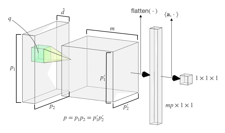
Figure 3: One-Hidden-Layer CNN for Theoretical Analysis

where $\bm{\zeta}$ abstractly represents all training parameters, $f(\mathbf{x},\cdot)$ denotes the output of the one-layer CNN for input $\mathbf{x}$, and $\mathcal{L}(\cdot)$ is the loss function. We make the following assumption on the training data and the CNN weight initialization.

Assumption 1.

(Training Data) Assume that for all $i\in[n]$, we have $\left\|\mathbf{x}_{i}\right\|_{F}=q^{-\frac{1}{2}}$ and $|y_{i}|\leq C$ for some constant $C$. Moreover, for all $i,i^{\prime}\in[n]$ we have $\mathbf{x}_{i}\neq\mathbf{x}_{i^{\prime}}$.

Note that the first part of this assumption is standard and can be satisfied by normalizing the data Du et al., (2018). For simplicity of the analysis, let $d:=q\hat{d}$.

Assumption 2.

(Initialization) $\mathbf{w}_{0,r}\sim\mathcal{N}\left(0,\kappa^{2}\mathbf{I}\right)$ and $a_{rj}\sim\left\{\pm\frac{1}{p\sqrt{m}}\right\}$ for $r\in[m]$ and $j\in[p]$.

We consider a simplified LoFT training scheme: assume that in the $t$th global iteration, we sample a set of $S$ masks, $\{\mathbf{m}_{t}^{(s)}\}_{s=1}^{S}$, for the filters, where each $\mathbf{m}_{t}^{(s)}\in\{0,1\}^{m}$. Let $m_{r,t}^{(s)}$ be the $r$th entry of $\mathbf{m}_{t}^{(s)}$. We assume that $m_{r,t}^{(s)}\sim\texttt{Bern}\left(\xi\right)$ for some $\xi\in(0,1]$ for all $s\in[S]$ and $r\in[m]$, with $m_{r,t}^{(s)}=1$ if the $r$th filter is trained in subnetwork $s$ and $m_{r,t}^{(s)}=1$ otherwise. Intuitively, $\xi$ is the probability that a filter is selected to be trained in a subnetwork. Let $\mathbf{m}_{t}^{(s)}$ be the $s$th column of the joint mask matrix $\mathbf{M}_{t}$. Then, each row $\mathbf{m}_{r,t}$ contains information of the subnetwork indices in which the $r$th filter is active. We further assume that the number of local iterations $\ell=1$.

Let $\{\mathbf{W}_{t}\}_{t=0}^{T}$ and $\{\hat{\mathbf{W}}_{t}\}_{t=0}^{T}$ be the weights in the trajectory of LoFT and GD, and let $\theta=\mathcal{P}\left(\vee_{s=1}^{S}\{m_{r}^{(s)}=1\}\right)=1-(1-\xi)^{S}$. Next, we show that the expected difference between the two is bounded as follows:

Theorem 1.

Let $f(\cdot,\cdot)$ be a one-hidden-layer CNN with the second layer weight fixed. Assume the number of hidden neurons satisfies $m=\Omega\left(\frac{n^{4}K^{2}}{\lambda_{0}^{4}\delta^{2}}\max\{n,d\}\right)$ and the step size satisfies $\eta=O\left(\frac{\lambda_{0}}{n^{2}}\right)$: Let Assumptions 1 and 2 be satisfied. Then, with probability at least $1-O\left(\delta\right)$ we have:

$${\color[rgb]{1,0,0}\mathbb{E}_{[\mathbf{M}_{T}]}\left[\left\|\mathbf{W}_{T}-\hat{\mathbf{W}}_{T}\right\|_{F}^{2}\right]}+$$

$$\quad\eta{\color[rgb]{0.5,0.5,0}\sum_{t=0}^{T-1}\mathbb{E}_{[\mathbf{M}_{T}]}\left[\left\|f\left(\mathbf{X},\mathbf{W}_{t}\right)-f\left(\mathbf{X},\hat{\mathbf{W}}_{t}\right)\right\|_{2}^{2}\right]}$$

$$\leq O\left({\color[rgb]{.5,0,.5}\tfrac{n^{2}\sqrt{d}}{\lambda_{0}^{2}\kappa m^{\frac{1}{4}}\sqrt{\delta}}}+{\color[rgb]{0,.5,.5}\tfrac{2\eta^{2}T\theta^{2}(1-\xi)\lambda_{0}}{S}}\right).$$

Remarks. Intuitively, this theorem states that the sum of the expected weight difference in the $T$th iteration (i.e., $\mathbb{E}_{[\mathbf{M}_{T}]}[\|\mathbf{W}_{T}-\hat{\mathbf{W}}_{T}\|_{F}^{2}]$) and the aggregation of the step-wise difference of the neural network output between LoFT and GD (i.e., $\sum_{t=0}^{T-1}\mathbb{E}_{[\mathbf{M}_{T}]}\|f\left(\mathbf{X},\mathbf{W}_{t}\right)-f\left(\mathbf{X},\hat{\mathbf{W}}_{t}\right)\|_{2}^{2}$) is bounded and controlled by the quantity on the right-hand side. In words, both the weights found by LoFT as well as the output of LoFT are close to the ones found by regular training. Notice that increasing the number of filters $m$ (term in violet color) and the number of subnetworks $S$ (term in teal color) will drive the bound of the summation to zero. For a more thorough discussion, as well as the proof, please see supplementary material. As a corollary of the theorem, we also show that LoFT training converges linearly upon to some neighborhood of the global minimum:

Corollary 1.

Let the same condition of theorem (1) holds, then we have:

$$\mathbb{E}_{[\mathbf{M}_{t-1}]}\left[\left\|f(\mathbf{X},\mathbf{W}_{t})-\mathbf{y}\right\|_{2}^{2}\right]\leq$$

$$\quad\left(1-\tfrac{\theta\eta\lambda_{0}}{2}\right)^{t}\left\|f(\mathbf{X},\mathbf{W}_{0})-\mathbf{y}\right\|_{2}^{2}+$$

$$\quad O\left(\tfrac{\xi(1-\xi)n^{3}d}{m\lambda_{0}^{2}}+\tfrac{n\kappa^{2}\left(\theta-\xi^{2}\right)}{S}\right).$$

We defer the proof for Theorem 1 and Corollary 1 to the appendix.

setting	Dense Model	methods	pruning ratio			Comm. cost	improv.
			80%	50%	30%
PreResNet-18 CIFAR-10	94.36	Gpipe-2	94.41	94.55		131.88G	$3.29\times$
		Local SGD-2	94.37	94.41		55.40G	$1.38\times$
		LoFT-2	93.97	94.11		40.02G	-
		Gpipe-4	94.41	94.55		659.42G	$10.21\times$
		Local SGD-4	94.52	94.81		110.80G	$1.72\times$
		LoFT-4	93.97	94.13		64.57G	-
PreResNet-34 CIFAR-10	93.51	Gpipe-2	93.93	94.38		131.88G	$2.01\times$
		Local SGD-2	94.77	95.13		105.93G	$1.61\times$
		LoFT-2	93.25	93.43		65.36G	-
		Gpipe-4	93.93	94.38		461.60G	$5.12\times$
		Local SGD-4	94.64	94.82		211.86G	$2.34\times$
		LoFT-4	93.89	94.02		90.17G	-
ResNet-34 CIFAR-10	93.22	Gpipe-2	93.69	93.81		131.88G	$2.01\times$
		Local SGD-2	94.49	94.74		105.93G	$1.61\times$
		LoFT-2	93.38	93.41		65.36G	-
		Gpipe-4	93.69	93.81		461.60G	$5.12\times$
		Local SGD-4	94.69	94.61		211.86G	$2.34\times$
		LoFT-4	93.41	93.60		90.17G	-
PreResNet-18 CIFAR-100	75.36	Gpipe-2	75.38	75.91		131.88G	$3.29\times$
		Local SGD-2	75.63	75.79		55.51G	$1.38\times$
		LoFT-2	75.99	76.65		40.03G	-
		Gpipe-4	75.38	75.91		659.42G	$10.21\times$
		Local SGD-4	75.50	75.44		111.03G	$1.72\times$
		LoFT-4	75.95	76.72		64.57G	-
PreResNet-34 CIFAR-100	76.57	Gpipe-2	76.72	77.09		131.88G	$2.01\times$
		Local SGD-2	75.26	76.18		106.05G	$1.61\times$
		LoFT-2	75.93	77.27		65.37G	-
		Gpipe-4	76.72	77.09		461.60G	$5.12\times$
		Local SGD-4	76.62	75.79		212.10G	$2.34\times$
		LoFT-4	75.77	76.79		90.17G	-
ResNet34 CIFAR-100	75.93	Gpipe-2	75.51	76.00		131.88G	$2.01\times$
		Local SGD-2	75.23	76.35		106.05G	$1.61\times$
		LoFT-2	76.11	77.07		65.37G	-
		Gpipe-4	75.51	76.00		461.60G	$5.12\times$
		Local SGD-4	76.19	76.81		212.10G	$2.34\times$
		LoFT-4	75.05	76.51		90.17G	-
PreResNet-18 ImageNet	70.71	Gpipe-2	66.71	69.14	70.29	20954.24G	$81.80\times$
		LoFT-2	65.41	69.12	69.64	256.62G
		Gpipe-4	66.71	69.14	70.29	52385.59G	$126.27\times$
		Local SGD-4	65.40	66.94	67.52	711.46G	$1.71\times$
		LoFT-4	65.60	68.93	69.77	414.84G

Table 1: Left: Fine-tuned accuracy for different pretraining methods at different pruning ratios. Dense Model corresponds to full CNN training without pruning. Right: Total communication costs (Comm.) of model parallel baseline (GPipe) Huang et al., (2019), Local SGD Stich, (2019) and LoFT during pretraining. Number after method name represents the number of parallel worker used. Orange color indicates that the method in comparison consumes at most $2\times$ communication bandwidth; red color indicates that the method in comparison consumes $>2\times$ communication bandwidth. Performance in teal color represents the best in terms of communication efficiency.

6 Experiments

We show that LoFT can preserve the winning tickets and non-trivially reduce costs during pretraining. First, we show that LoFT recovers winning tickets under various settings for all pruning levels with a significant reduction in communication cost compared to other model-parallel methods. Second, we illustrate that LoFT does not recover the winning tickets by chance: LoFT converges to winning tickets faster and provide better tickets for all pretraining length.

Experimental Setup. We consider the workflow of pretraining for 20 epochs and fine-tuning for 90 epochs. We consider three CNNs: PreActResNet-18, PreActResNet-34 He et al., (2016), and WideResNet-34 Zagoruyko and Komodakis, (2016) to characterize our performance on models of different sizes and structures. We test these settings on the CIFAR-10, CIFAR-100, and ImageNet datasets.

For our baseline, we compare with a standard model-parallel algorithm Gpipe Huang et al., (2019), where we distribute layers of a network to different workers. We note that model-parallel algorithms are equivalent to training the whole model on a single large GPU. However, since LoFT partitions the model based on the number of workers and utilizes independent training for each subnetwork, it is not equivalent to full model training, and the final performance will be different based on the number of workers we use. This is where our savings in communication cost come from, and why it is non-trivial for LoFT to even match the performance of other methods. We also compare against the standard data parallel local SGD methodology Stich, (2019). (Due to limitation of computing resource, we only experiment on 4-worker Local SGD on Imagenet dateset as the focus is on comparing with other model-parallel methods.)

We used two different pruning ratios: i.e., 50%, and 80% pruning ratios to profile performance under normal and over-pruning settings, respectively. For ImageNet, we additionally consider a pruning ratio 30%, since networks are usually pruned less in this setting Li et al., (2016). Here the pruning ratio $p\%$ represents that for each set of filters $\mathcal{F}_{i}$, we remove the bottom $p\%$ of the filters by its $\ell_{2}$-norm $\left\|\mathcal{F}_{i,j}\right\|_{2}$, as described above. We do not prune the layers that are known to be most sensitive to pruning: this is skipping the first residual block and the strided convolutional blocks, according to Liu et al., (2018); Li et al., (2016).

There are methods with more specific pruning schedules, or different pruning ratios for different layers Li et al., (2016). Here, we do not delve into layer-specific pruning or parameter tuning and only use one shared pruning ratio. The focus is on the general quality of the winning ticket selected from LoFT with other model-parallel methods.

Implementation Details. We provide a PyTorch implementation of LoFT using the NCCL distributed communication package for training ResNet He et al., (2015) and WideResNet Zagoruyko and Komodakis, (2016) architectures. Experiments are conducted on a node with 8 NVIDIA Tesla V100-PCIE-32G GPUs, a 24-core Intel(R) Xeon(R) Gold 5220R CPU 2.20GHz, 1.5 TB of RAM.

LoFT recovers winning tickets with lower communication cost. Table 1 shows the performance comparison for LoFT, Local SGD (data parallel) and Gpipe (model parallel) under various settings. We also include the performance of the Dense Model, where the network is trained as-is with the same setting without any pruning. We can see that across different model sizes, network structures, pruning ratios, and datasets, LoFT finds comparable or better tickets compared to other model-/data-parallel pretraining methods, while providing sizable savings in communication cost. Note that LoFT partitions the model into smaller subnetworks; so it is non-trivial that e.g., the 4-worker case leads to the same final accuracy, as compared to the 2-worker or the full model cases.

While LoFT inherits the memory efficiency from model-parallel training methods, it further reduces the communication cost from $1.38\times$ up to $126.27\times$, as shown in Table 1. Similar behavior is observed in comparison to data-parallel training methids: the gains in communication overhead range from $1.38\times$ to $2.34\times$. We note though that in this case, for a sufficiently large model, it could be the case that the model does not fit in the workers’ GPU RAM; in contrast, GPipe and LoFT allow efficient training of larger neural network models, by definition. This overall improvement by LoFT is achieved by $i)$ changing the way of decomposing the network such that each worker can host an independent subnetwork and train locally without communication, which greatly reduces the communication frequency; and $ii)$ each worker only exchange the weight of the subnetwork after each round of local training instead of transmitting activation maps and gradients.

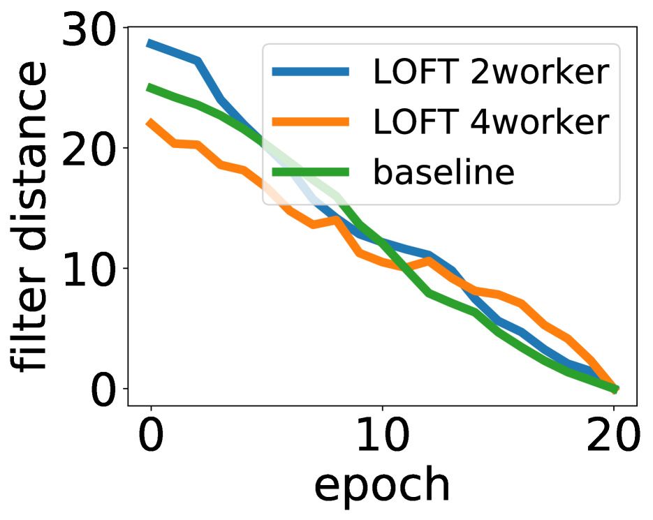
(a) CIFAR10

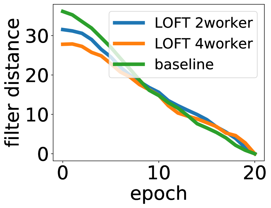
(b) CIFAR100

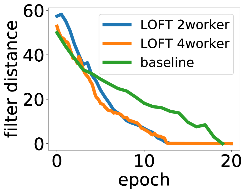
(c) ImageNet

Figure 4: filter distance with respect to final ticket throughout pretraining process

LoFT converges faster provides better tickets throughout pretraining.

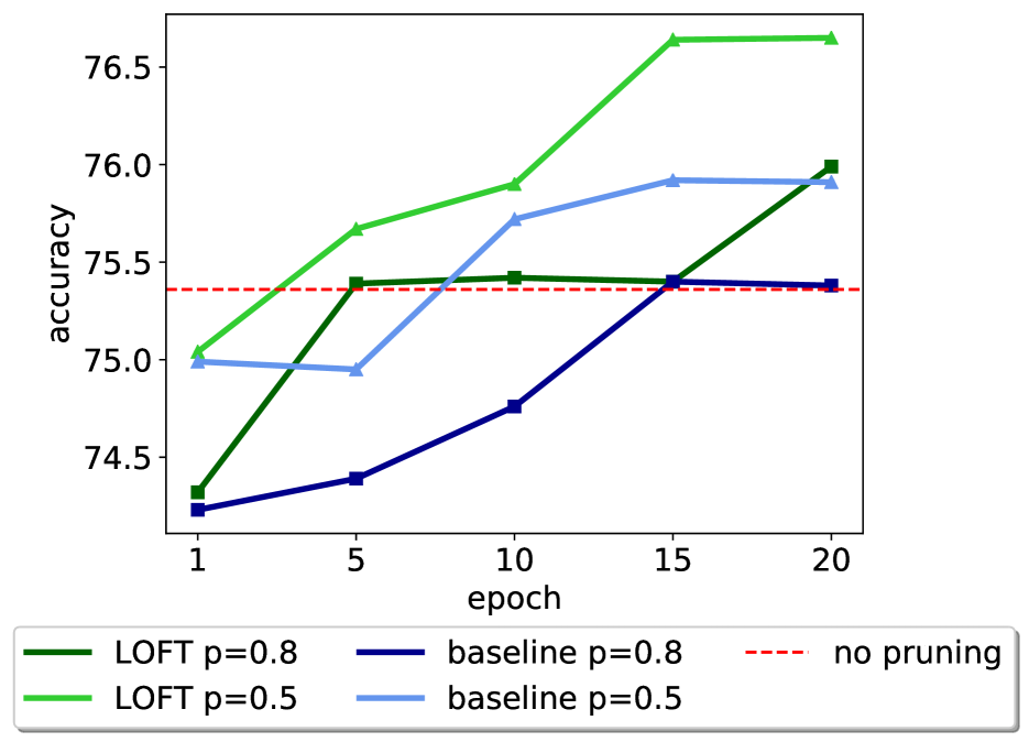
Figure 5: Final accuracy after $i)$ selecting a ticket drawn at different epochs for training (x-axis), and $ii)$ further training the selected ticket for 90 epochs, as described in main text. This plot considers the CIFAR100 case.

We provide a closer look into some empirical results that showcase LoFT’s ability to provide better tickets early in training. In Figure 5, we sampled different tickets (every 5 epochs) from the first 20 epochs in pretraining, and report all their final accuracy after fine tuning. We can see that LoFT yields better tickets (higher final accuracy) compared to Gpipe baseline. This shows that LoFT does not rely on a particular pretraining length and provides better tickets throughout pretraining.

To better compare the filter convergence, we calculated the filter distance between filters in the final epoch and filters in the previous pretraining epochs, As described above, the filter distance measures the change in the rankings of the filters. Larger filter distance means the important filters have not yet been identified as the top rank filters. As shown in Figure 4. LoFT quickly and monotonically decreases the filter distance to the filters in the final epoch, showing it is able to efficiently identify and preserve the correct winning ticket. In the more challenging ImageNet dataset, LoFT can decrease the filter distance faster than the baseline pretraining, which suggests LoFT is a better way to find the winning ticket by providing some acceleration in filter convergence.

7 Related Work

Algorithms for distributed training may be categorized into model parallel and data parallel methodologies. In the former Dean et al., (2012); Hadjis et al., (2016), portions of the NN are partitioned across different compute nodes, while, in the latter Farber and Asanovic, (1997); Raina et al., (2009), the complete NN is updated with different data on each compute node. Due to its ease-of-implementation, data parallel training is the most popular distributed training framework in practice.

As data parallelism needs to update the whole model on each worker –which still results in a large memory and computational cost– researchers utilize model parallelism, such as Gpipe Huang et al., (2019), to reduce the per node computational burden. On the the other hand, pure model parallelism needs to synchronize at every training iteration to exchange intermediate activations and gradient information between workers, resulting in high communication costs.

Following recent work that efficiently discovers winning tickets early in the training process You et al., (2019), our methodology further improves the efficiency of LTH by extending its application to communication-efficient, distributed training. Furthermore, by allowing significantly larger networks during pretraining, we enable the discovery of higher-performing winning tickets.

Previous work by You et al., (2019) proposed mask distance as a tool for identifying winning ticket early in the training process. Mask distance considers the Hamming distance of the 0-1 pruned mask on batch normalization (BN) layers. While similar in motivation, our filter distance criteria is fundamentally different. The two methods aim to capture totally different part of the training dynamic. Filter distance profiles the ordering of convolutional filters, while mask distance captures the activation of batch normalization layers. Filter distance models pruning process as a ranking whereas mask distance models it as a binary mask. Furthermore, filter distance is a consistent measurement that does not depend on the pruning ratio whereas mask distance can only be calculated with respect to a specific pruning ratio.

8 Conclusion and Discussion

LoFT is a novel model-parallel pretraining algorithm that is both memory and communication efficient. Moreover, experiments show that LoFT can discover tickets faster or comparable than model-parallel training, and discover tickets with higher or comparable final accuracy. An immediate future work is, with more computation budget, testing LoFT with larger models and more challenging datasets. We are also curious how will the accuracy scale as we use more workers. Finally, it is also an open question whether we can further automate the pretraining process by using some adaptive stopping criteria to stop pretraining to identify winning tickets without hyperparameter tuning.

Appendix A Detailed Mathematical Formulation of LoFT

detailed_math_form For a vector $\mathbf{v}$, $\left\|\mathbf{v}\right\|_{2}$ denotes its Euclidean ($\ell_{2}$) norm. For a matrix $\mathbf{V}$, $\left\|\mathbf{V}\right\|_{F}$ denotes its Frobenius norm. We use $\mathcal{P}\left(\cdot\right)$ to denote the probability of an event, and $\mathbb{I}\left\{\cdot\right\}$ to denote the indicator function. For two vectors $\mathbf{v}_{1},\mathbf{v}_{2}$, we use the simplified notation $\mathbb{I}\left\{\mathbf{v}_{1};\mathbf{v}_{2}\right\}:=\mathbb{I}\left\{\left\langle\mathbf{v}_{1},\mathbf{v}_{2}\right\rangle\geq 0\right\}$. Given that the mask in iteration $t$ is $\mathbf{M}_{t}$, we denote $\mathbb{E}_{[\mathbf{M}_{t}]}\left[\cdot\right]=\mathbb{E}_{\mathbf{M}_{0},\dots,\mathbf{M}_{t}}\left[\cdot\right]$.

Recall that the CNN considered in this paper has the form

$$f(\mathbf{x},\theta)=\left\langle\mathbf{a},\sigma\left(\mathbf{W}_{1}\hat{\phi}\left(\mathbf{x}\right)\right)\right\rangle$$

Denote $\hat{\mathbf{x}}=\hat{\phi}\left(\mathbf{x}\right)$. Essentially, this patching operator applies to each channel, with the effect of extending each pixel to a set of pixels around it. So we denote $\hat{\mathbf{x}}_{i}^{(j)}\in\mathbb{R}^{q\hat{d}}$ as the extended $j$th pixel across all channels in the $i$th sample. For each transformed sample, we have that $\left\|\hat{\mathbf{x}}_{i}\right\|_{F}\leq\sqrt{q}\left\|\mathbf{x}_{i}\right\|_{F}$. We simplify the CNN output as

$$f(\hat{\mathbf{x}},\mathbf{W})=\left\langle\mathbf{a},\sigma\left(\mathbf{W}\otimes\hat{\mathbf{x}}\right)\right\rangle=\sum_{r=1}^{m_{1}}\sum_{j=1}^{p}a_{rj}\sigma\left(\left\langle\hat{\mathbf{x}}^{(j)},\mathbf{w}_{r}\right\rangle\right)$$

In this way, the formulation of CNN reduces to MLP despite a different form of input data $\hat{\mathbf{x}}$ and an additional dimension of aggregation in the second layer. We consider train neural network $f$ on the mean squared error (MSE)

$$\mathcal{L}\left(\mathbf{W}\right)=\left\|f\left(\hat{\mathbf{X}},\mathbf{W}\right)-\mathbf{y}\right\|_{2}^{2}=\sum_{i=1}^{n}\left(f\left(\hat{\mathbf{x}}_{i},\mathbf{W}\right)-y_{i}\right)^{2}$$

Now, we consider an $S$-worker LoFT scheme. The subnetwork by filter-wise partition is given by

$$f_{\mathbf{m}^{(s)}}\left(\hat{\mathbf{x}},\mathbf{W}\right)=\sum_{r=1}^{m_{1}}\sum_{j=1}^{p}m^{(s)}_{r}a_{rj}\sigma\left(\left\langle\hat{\mathbf{x}}^{(j)},\mathbf{w}_{r}\right\rangle\right)$$

Trained on the regression loss, the surrogate gradient is given by

$$\nabla_{\mathbf{w}_{r}}\mathcal{L}_{\mathbf{m}^{(s)}}\left(\mathbf{W}\right)=m^{(s)}_{r}\sum_{i=1}^{n}\sum_{j=1}^{p}\left(f_{\mathbf{m}^{(s)}}\left(\hat{\mathbf{x}}_{i},\mathbf{W}\right)-y_{i}\right)a_{rj}\hat{\mathbf{x}}_{i}^{(j)}\mathbb{I}\left\{\hat{\mathbf{x}}_{i}^{(j)};\mathbf{w}_{r}\right\}$$

We correspondingly scale the whole network function

$$f\left(\hat{\mathbf{x}},\mathbf{W}\right)=\xi\sum_{r=1}^{m}\sum_{j=1}^{p}a_{rj}\sigma\left(\left\langle\hat{\mathbf{x}}_{i}^{(j)},\mathbf{w}_{r}\right\rangle\right)$$

Assuming it is also training on the MSE, we write out its gradient as

$$\nabla_{\mathbf{w}_{r}}\mathcal{L}\left(\mathbf{W}\right)=\xi\sum_{i=1}^{n}\sum_{j=1}^{n}\left(f\left(\hat{\mathbf{x}}_{i},\mathbf{W}\right)-y_{i}\right)a_{rj}\hat{\mathbf{x}}_{i}^{(j)}\mathbb{I}\left\{\hat{\mathbf{x}}_{i}^{(j)};\mathbf{w}_{r}\right\}$$

In this work, we consider the one-step LoFT training, given by

$$\mathbf{w}_{r,t+1}=\mathbf{w}_{r,t}-\eta\frac{N_{r,t}^{\perp}}{N_{r,t}}\sum_{s=1}^{S}\nabla_{\mathbf{w}_{r}}\mathcal{L}_{\mathbf{m}_{t}^{(s)}}\left(\mathbf{W}_{r,t}\right)$$

Here, let $N_{r,t}=\max\left\{\sum_{s=1}^{S}m_{r,t}^{(s)},1\right\}$, and $N_{r,t}^{\perp}=\min\left\{\sum_{s=1}^{S}m_{r,t}^{(s)},1\right\}$. Intuitively, $N_{r,t}$ denote the ”normalizer” that we will divide the sum of the gradients from all subnetworks with, and $N_{r,t}^{\perp}$ denote the indicator of whether filter $r$ is trained in at least one subnetwork. Let $\theta=\mathcal{P}\left(N_{r,t}^{\perp}=1\right)=1-(1-\xi)^{p}$, denoting the probability that at least one of $\left\{m_{r,t}^{(s)}\right\}_{s=1}^{S}$ is one. Denote $u_{t}^{(i)}=f\left(\hat{\mathbf{x}}_{i},\mathbf{W}_{t}\right)$. For further convenience of our analysis, we define

$$\tilde{u}_{r,t}^{(i)}=\frac{N_{r,t}^{\perp}}{N_{r,t}}\sum_{s=1}^{S}m_{r,t}^{(s)}\hat{u}_{t}^{(s,i)};\quad\mathbf{g}_{r,t}=\frac{N_{r,t}^{\perp}}{N_{r,t}}\sum_{s=1}^{S}\nabla_{\mathbf{w}_{r}}\mathcal{L}_{\mathbf{m}_{t}^{(s)}}\left(\mathbf{W}_{t}\right)$$

Then the LoFT training has the form

$$\mathbf{w}_{r,t+1}=\mathbf{w}_{r,t}-\eta\mathbf{g}_{r,t};\quad\mathbf{g}_{r,t}=\sum_{i=1}^{n}\sum_{j=1}^{p}a_{rj}\left(\tilde{u}_{r,t}^{(i)}-N_{r,t}^{\perp}y_{i}\right)\hat{\mathbf{x}}_{i}^{(j)}\mathbb{I}\left\{\hat{\mathbf{x}}_{i}^{(j)};\mathbf{w}_{r,t}\right\}$$

Suppose that assumptions in main text hold. Then for all $i\in[n]$ we have $\left\|\mathbf{x}_{i}\right\|_{F}=q^{\frac{1}{2}}$, and for all $i,i^{\prime}\in[n]$ such that $i\neq i^{\prime}$, we have $\mathbf{x}_{i}\neq\mathbf{x}_{i^{\prime}}$. As in previous work (Du et al.,, 2018), we have $\left\|\hat{\mathbf{x}}_{i}\right\|_{F}\leq\sqrt{q}\left\|\mathbf{x}_{i}\right\|_{F}\leq 1$. Thus, for all $j\in[p]$ we have $\left\|\hat{\mathbf{x}}_{i}^{(j)}\right\|\leq 1$. Moreover, since $\mathbf{x}_{i}\neq\mathbf{x}_{i^{\prime}}$ for $i\neq i^{\prime}$, we then have $\hat{\mathbf{x}}_{i}\neq\hat{\mathbf{x}}_{i^{\prime}}$, which implies that $\hat{\mathbf{x}}_{i}^{(j)}\neq\hat{\mathbf{x}}_{i^{\prime}}^{(j)}$ for all $i\neq i^{\prime}$ and $j\in[p]$.

Appendix B One-Step LoFT Convergence

In this section, our goal is to prove and extended version of Corollary 1 in the main text, as a new theorem. We first state the extended version here, and proceed to prove it.

Theorem 2.

Let $f$ be a one-hidden-layer CNN with the second layer weight fixed. Assume the number of hidden neurons satisifes $m=\Omega\left(\frac{n^{3}K^{2}}{\lambda_{0}^{4}\delta^{2}\kappa^{2}}\max\{n,d\}\right)$ and the step size satisfies $\eta=O\left(\frac{\lambda_{0}}{n^{2}}\right)$. Let Assumption 1 and 2 be satisfied. Then with probability at least $1-O\left(\delta\right)$ we have that

$$\mathbb{E}_{[\mathbf{M}_{t-1}]}\left[\left\|\mathbf{u}_{t}-\mathbf{y}\right\|_{2}^{2}\right] \leq\left(1-\frac{\theta\eta\lambda_{0}}{2}\right)^{t}\left\|\mathbf{u}_{0}-\mathbf{y}\right\|_{2}^{2}+O\left(\frac{\xi^{2}(1-\xi)^{2}n^{3}d}{m\lambda_{0}^{2}}+\frac{n\kappa^{2}\left(\theta-\xi^{2}\right)}{S}\right)$$

and the weight perturbation is bounded by

$$\mathbb{E}_{[\mathbf{M}_{t-1}]}\left[\left\|\mathbf{w}_{r,t}-\mathbf{w}_{r,0}\right\|_{2}\right]\leq O\left(\lambda_{0}^{-1}\sqrt{\frac{n}{m}}\right)\left\|\mathbf{u}_{0}-\mathbf{y}\right\|_{2}+$$

$$\eta\theta T\cdot O\left(\frac{\xi(1-\xi)n^{2}\sqrt{d}}{m\lambda_{0}}+n\kappa\sqrt{\frac{\theta-\xi^{2}}{mS}}\right)$$

This is essentially a multi-sample drop-out proof for one-hidden-layer MLP, with an additional summation over the pixels $j\in[p]$. For completeness we present the proof here. We care about the MSE computed on the scaled full network

$$u_{k}^{(i)}=\xi\sum_{r=1}^{m}\sum_{j=1}^{p}a_{rj}\sigma\left(\left\langle\hat{\mathbf{x}}_{i}^{(j)},\mathbf{w}_{r,t}\right\rangle\right);\quad\mathcal{L}\left(\mathbf{W}_{t}\right)=\left\|\mathbf{u}_{t}-\mathbf{y}\right\|_{2}^{2}$$

Performing gradient descent on this scaled full network involves computing

$$\nabla_{\mathbf{w}_{r}}\mathcal{L}\left(\mathbf{W}_{t}\right)=\xi\sum_{i=1}^{n}\sum_{j=1}^{p}\left(u_{t}^{(i)}-y_{i}\right)a_{rj}\hat{\mathbf{x}}_{i}^{(j)}\mathbb{I}\left\{\hat{\mathbf{x}}_{i}^{(j)};\mathbf{w}_{r,t}\right\}$$

B.1 Change of Activation Pattern

Let $R$ be some fixed scale. For analysis convenience, we denote

$$A_{ir}^{(j)}=\left\{\exists\mathbf{w}:\left\|\mathbf{w}-\mathbf{w}_{r,0}\right\|_{2}\leq R;\mathbb{I}\left\{\hat{\mathbf{x}}_{i}^{(j)};\mathbf{w}\right\}\neq\mathbb{I}\left\{\hat{\mathbf{x}}_{i}^{(j)};\mathbf{w}_{r,0}\right\}\right\}$$

Note that $A_{ir}^{(j)}$ happens if and only if $\left|\left\langle\hat{\mathbf{x}}_{i}^{(j)},\mathbf{w}_{r,0}\right\rangle\right|<R$. Therefore $\mathbb{P}\left(A_{ir}^{(j)}\right)<\frac{2R}{\kappa\sqrt{2\pi}}$. Denote

$$P_{ij}=\left\{r\in[m]:\neg A_{ir}^{(j)}\right\};\quad P_{ij}^{\perp}=[m]\setminus P_{ij}$$

The next lemma shows the magnitude of $P_{ij}^{\perp}$

Lemma 1.

Let $m=\Omega\left(R^{-1}\log\frac{np}{\delta}\right)$. Then with probability at least $1-O(\delta)$ it holds for all $i\in[n]$ and $j\in[p]$ that

$$\left|P_{ij}^{\perp}\right|\leq 3m\kappa^{-1}R$$

Proof.

The magnitude of $P_{ij}^{\perp}$ satisfies

$$\left|P_{ij}^{\perp}\right|=\sum_{r=1}^{m}\mathbb{I}\left\{A_{ir}^{(j)}\right\}$$

The indicator function $\mathbb{I}\left\{A_{ir}^{(j)}\right\}$ has bounded first and second moment

$$\mathbb{E}_{\mathbf{W}}\left[\mathbb{I}\left\{A_{ir}^{(j)}\right\}\right]=\mathbb{P}\left(A_{ir}^{(j)}\right) \leq\frac{2R}{\kappa\sqrt{2\pi}}$$

$$\mathbb{E}_{\mathbf{W}}\left[\left(\mathbb{I}\left\{A_{ir}^{(j)}-\mathbb{E}_{\mathbf{W}}\left[\mathbb{I}\left\{A_{ir}^{(j)}\right\}\right]\right\}\right)^{2}\right] \leq\mathbb{E}_{\mathbf{W}}\left[\mathbb{I}\left\{A_{ir}^{(j)}\right\}^{2}\right]\leq\frac{2R}{\kappa\sqrt{2\pi}}$$

This allows us to apply the Berstein Inequality to get that

$$\mathbb{P}\left(\sum_{r=1}^{m}\mathbb{I}\left\{A_{ir}^{(j)}\right\}>\frac{2mR}{\kappa\sqrt{2\pi}}+mt\right)<\exp\left(-\frac{m\kappa t^{2}\sqrt{2\pi}}{8\left(1+\frac{t}{3}\right)R}\right)$$

Therefore, with probability at least $1-np\exp\left(-m\kappa^{-1}R\right)$ it holds for all $i\in[n]$ and $j\in[p]$ that

$$\left|P_{ij}^{\perp}\right|=\sum_{r=1}^{m}\mathbb{I}\left\{A_{ir}^{(j)}\right\}\leq 3m\kappa^{-1}R$$

Letting $m=\Omega\left(R^{-1}\log\frac{np}{\delta}\right)$ gives that the success probability is at least $1-O(\delta)$. ∎

B.2 Initialization Scale

Let $\mathbf{w}_{0,r}\sim\mathcal{N}\left(0,\kappa^{2}\mathbf{I}\right)$ and $a_{j}\sim\left\{-\frac{1}{p\sqrt{m}},\frac{1}{p\sqrt{m}}\right\}$ for all $r\in[m]$ and $j\in[p]$. We cite some results from prior work to deal with the initialization scale

Lemma 2.

Suppose $\kappa\leq 1,R\leq\kappa\sqrt{\frac{d}{32}}$. With probability at least $1-e^{md/32}$ we have that

$$\|W_{0}\|_{F}\leq\kappa\sqrt{2md}-\sqrt{m}R$$

Lemma 3.

Assume $\kappa\leq 1$ and $R\leq\frac{\kappa}{\sqrt{2}}$. With probability at least $1-ne^{-\frac{m}{32}}$ over initialization, it holds for all $i\in[n]$ that

$$\sum_{r=1}^{m}\left\langle\mathbf{w}_{0,r},\mathbf{x}_{i}\right\rangle^{2}\leq 2m\kappa^{2}-mR^{2}$$

$$\sum_{i=1}^{n}\sum_{r=1}^{m}\left\langle\mathbf{w}_{0,r},\mathbf{x}_{i}\right\rangle^{2}\leq 2mn\kappa^{2}-mnR^{2}$$

Moreover, we can bound the initial MSE

Lemma 4.

Assume that for all $i\in[n]$, $y_{i}$ satisfies $|y_{i}|\leq C$ for some $C>0$. Then, we have

$$\mathbb{E}_{\mathbf{W}_{0},\hat{\mathbf{a}}}\left[\|\mathbf{y}-\mathbf{u}_{0}\|_{2}^{2}\right]\leq\left(p^{-1}+C^{2}\right)n$$

Proof.

It is obvious that $\mathbb{E}_{\mathbf{W}_{0},\hat{\mathbf{a}}}\left[u_{0}^{(i)}\right]=0$ for all $i\in[n]$. Moreover,

$$\mathbb{E}_{\mathbf{W}_{0},\hat{\mathbf{a}}}\left[u_{0}^{(i)2}\right] =\sum_{r,r^{\prime}=1}^{m}\sum_{j,j^{\prime}=1}^{p}\mathbb{E}_{\hat{\mathbf{a}}}\left[a_{rj}a_{r^{\prime}j^{\prime}}\right]\mathbb{E}_{\mathbf{W}_{0}}\left[\sigma\left(\left\langle\hat{\mathbf{x}}_{i}^{(j)},\mathbf{w}_{0,r}\right\rangle\right)\sigma\left(\left\langle\hat{\mathbf{x}}_{i}^{(j^{\prime})},\mathbf{w}_{0,r}\right\rangle\right)\right]$$

$$=\frac{1}{p^{2}m}\sum_{r=1}^{m}\sum_{j=1}^{p}\mathbb{E}_{\mathbf{W}_{0}}\left[\sigma\left(\left\langle\hat{\mathbf{x}}_{i}^{(j)},\mathbf{w}_{0,r}\right\rangle\right)^{2}\right]$$

$$\leq\frac{1}{p^{2}m}\sum_{r=1}^{m}\sum_{j=1}^{p}\mathbb{E}_{\mathbf{W}_{0}}\left[\left\langle\hat{\mathbf{x}}_{i}^{(j)},\mathbf{w}_{0,r}\right\rangle\right]$$

$$\leq p^{-1}$$

Therefore

$$\mathbb{E}_{\mathbf{W}_{0},\hat{\mathbf{a}}}\left[\left\|\mathbf{u}_{0}-\mathbf{y}\right\|_{2}^{2}\right]=\sum_{i=1}^{n}\mathbb{E}_{\mathbf{W}_{0},\hat{\mathbf{a}}}\left[\left(u_{0}^{(i)}-y_{i}\right)_{2}^{2}\right]=\sum_{i=1}^{n}\left(\mathbb{E}_{\mathbf{W}_{0},\hat{\mathbf{a}}}\left[u_{0}^{(i)2}\right]+y_{i}^{2}\right)\leq\left(p^{-1}+C^{2}\right)n$$

∎

B.3 Kernel Analysis

The neural tangent kernel is defined to be the inner product of the gradient with respect to the neural network output. We let the finite-width NTK be defined as

$$\mathbf{H}(t)_{ii^{\prime}}=\sum_{r=1}^{m}\sum_{j,j^{\prime}=1}^{p}a_{rj}a_{rj^{\prime}}\left\langle\hat{\mathbf{x}}_{i}^{(j)},\hat{\mathbf{x}}_{i^{\prime}}^{(j^{\prime})}\right\rangle\mathbb{I}\left\{\hat{\mathbf{x}}_{i}^{(j)};\mathbf{w}_{r,t}\right\}\mathbb{I}\left\{\hat{\mathbf{x}}_{i^{\prime}}^{(j^{\prime})};\mathbf{w}_{r,t}\right\}$$

Moreover, let the infinite width NTK be defined as

$$\mathbf{H}^{\infty}_{ii^{\prime}}=\frac{1}{p^{2}}\sum_{j=1}^{p}\left\langle\hat{\mathbf{x}}_{i}^{(j)},\hat{\mathbf{x}}_{i^{\prime}}^{(j)}\right\rangle\mathbb{E}_{\mathbf{w}\sim\mathcal{N}\left(0,\mathbf{I}\right)}\left[\mathbb{I}\left\{\hat{\mathbf{x}}_{i}^{(j)};\mathbf{w}\right\}\mathbb{I}\left\{\hat{\mathbf{x}}_{i^{\prime}}^{(j)};\mathbf{w}\right\}\right]$$

Let $\lambda_{0}=\lambda_{\min}\left(\mathbf{H}^{\infty}\right)$. Note that since $\hat{\mathbf{x}}_{i}\not\parallel\hat{\mathbf{x}}_{i^{\prime}}$ for $i\neq i^{\prime}$. Thus $\hat{\mathbf{x}}_{i}^{(j)}\not\parallel\hat{\mathbf{x}}_{i^{\prime}}^{(j)}$ for $i\neq i^{\prime}$. () shows that the matrix $\hat{\mathbf{H}}(j)$ , as defined below, is positive definite for all $j\in[p]$

$$\hat{\mathbf{H}}(j)_{ii^{\prime}}^{\infty}=\left\langle\hat{\mathbf{x}}_{i}^{(j)},\hat{\mathbf{x}}_{i^{\prime}}^{(j)}\right\rangle\mathbb{E}_{\mathbf{w}\sim\mathcal{N}\left(0,\mathbf{I}\right)}\left[\mathbb{I}\left\{\hat{\mathbf{x}}_{i}^{(j)};\mathbf{w}\right\}\mathbb{I}\left\{\hat{\mathbf{x}}_{i^{\prime}}^{(j)};\mathbf{w}\right\}\right]$$

Since $\mathbf{H}^{\infty}=p^{-2}\sum_{j=1}^{p}\hat{\mathbf{H}}(j)^{\infty}$, we have that $\mathbf{H}^{\infty}$ is positive definite and thus $\lambda_{0}>0$. The following lemma shows that the NTK remains positive definite throughout training.

Lemma 5.

Let $m=\Omega\left(\lambda_{0}^{-2}n^{2}\log\frac{n}{\delta}\right)$. If for all $r\in[m]$ and all $t$ we have $\left\|\mathbf{w}_{r,t}-\mathbf{w}_{r,0}\right\|_{2}\leq R:=O\left(\frac{\kappa\lambda_{0}}{n}\right)$. Then with probability at least $1-\delta$ we have that for all $t$

$$\lambda_{\min}\left(\mathbf{H}(t)\right)\geq\frac{\lambda_{0}}{2}$$

Proof.

To start, we notice that for all $r\in[m]$

$$\mathbb{E}_{\mathbf{W}_{0},\mathbf{a}} \left[\sum_{j,j^{\prime}=1}^{p}a_{rj}a_{rj^{\prime}}\mathbb{I}\left\{\hat{\mathbf{x}}_{i}^{(j)};\mathbf{w}_{r,0}\right\}\mathbb{I}\left\{\hat{\mathbf{x}}_{i^{\prime}}^{(j^{\prime})};\mathbf{w}_{r,0}\right\}\right]$$

$$\quad\quad\quad=\frac{1}{p^{2}m}\mathbb{E}_{\mathbf{w}\sim\mathcal{N}(0,\mathbf{I})}\left[\mathbb{I}\left\{\hat{\mathbf{x}}_{i}^{(j)};\mathbf{w}\right\}\mathbb{I}\left\{\hat{\mathbf{x}}_{i^{\prime}}^{(j)};\mathbf{w}\right\}\right]$$

Moreover, we have that

$$\left|\sum_{j,j^{\prime}=1}^{p}a_{rj}a_{rj^{\prime}}\left\langle\hat{\mathbf{x}}_{i}^{(j)},\hat{\mathbf{x}}_{i^{\prime}}^{(j^{\prime})}\right\rangle\mathbb{I}\left\{\hat{\mathbf{x}}_{i}^{(j)};\mathbf{w}_{r,0}\right\}\mathbb{I}\left\{\hat{\mathbf{x}}_{i^{\prime}}^{(j^{\prime})};\mathbf{w}_{r,0}\right\}\right|\leq 1$$

Thus, we can apply Hoeffding’s inequality with bounded random variable to get that

$$\mathbb{P}\left(\left|\mathbf{H}(0)_{i,i^{\prime}}-\mathbf{H}^{\infty}_{i,i^{\prime}}\right|\geq t\right)\leq 2\exp\left(-mt^{2}\right)$$

Therefore, with probability at least $1-O(\delta)$ it holds that for all $i,i^{\prime}\in[n]$

$$\left|\mathbf{H}(0)_{i,i^{\prime}}-\mathbf{H}^{\infty}_{i,i^{\prime}}\right|\leq\frac{\log\frac{n}{\delta}}{\sqrt{m}}$$

which implies that

$$\left\|\mathbf{H}(0)-\mathbf{H}^{\infty}\right\|\leq\left\|\mathbf{H}(0)-\mathbf{H}^{\infty}\right\|_{F}\leq\frac{n\left(\log\delta^{-1}+\log n\right)}{\sqrt{m}}$$

As long as $m=\Omega\left(\lambda_{0}^{-2}n^{2}\log\frac{n}{\delta}\right)$ we will have

$$\left\|\mathbf{H}(t)-\mathbf{H}^{\infty}\right\|\leq\frac{\lambda_{0}}{4}$$

Now we move on to bound $\left\|\mathbf{H}(t)-\mathbf{H}(0)\right\|$. We have that

$$\mathbf{H}(t)_{i,i^{\prime}}-\mathbf{H}(0)_{i,i^{\prime}}=\sum_{r=1}^{m}\sum_{j,j^{\prime}=1}^{p}a_{rj}a_{rj^{\prime}}\left\langle\hat{\mathbf{x}}_{i}^{(j)},\hat{\mathbf{x}}_{i^{\prime}}^{(j^{\prime})}\right\rangle z_{r,i,i^{\prime}}^{(j,j^{\prime})}$$

with

$$z_{r,i,i^{\prime}}^{(j,j^{\prime})}=\mathbb{I}\left\{\hat{\mathbf{x}}_{i}^{(j)};\mathbf{w}_{r,t}\right\}\mathbb{I}\left\{\hat{\mathbf{x}}_{i^{\prime}}^{(j^{\prime})};\mathbf{w}_{r,t}\right\}-\mathbb{I}\left\{\hat{\mathbf{x}}_{i}^{(j)};\mathbf{w}_{r,0}\right\}\mathbb{I}\left\{\hat{\mathbf{x}}_{i^{\prime}}^{(j^{\prime})};\mathbf{w}_{r,0}\right\}$$

We observe that $|z_{r,i,i^{\prime}}^{(j,j^{\prime})}|$ only if $A_{ir}^{(j)}\vee A_{i^{\prime}r}^{(j^{\prime})}$. Therefore

$$\mathbb{E}_{\mathbf{W}}\left[z_{r,i,i^{\prime}}^{(j,j^{\prime})}\right]\leq\mathbb{P}\left(A_{ir}^{(j)}\right)+\mathbb{P}\left(A_{i^{\prime}r}^{(j^{\prime})}\right)\leq\frac{4R}{\kappa\sqrt{2\pi}}$$

For the case $j=j^{\prime}$, we first notice that

$$\mathbb{E}_{\mathbf{W}}\left[\left(z_{r,i,i^{\prime}}^{(j,j^{\prime})}-\mathbb{E}_{\mathbf{W}}\left[z_{r,i,i^{\prime}}^{(j,j^{\prime})}\right]\right)^{2}\right]\leq\mathbb{E}_{\mathbf{W}}\left[z_{r,i,i^{\prime}}^{(j,j^{\prime})2}\right]\leq\frac{4R}{\kappa\sqrt{2\pi}}$$

Thus, applying Berstein Inequality to the case $j=j^{\prime}$ we have that

$$\mathbb{P}\left(\sum_{r=1}^{m}z_{r,i,i^{\prime}}^{(j,j)}\geq m\left(\mathbb{E}_{\mathbf{W}}\left[z_{r,i,i^{\prime}}^{(j,j^{\prime})}\right]+t\right)\right)\leq\exp\left(-\frac{\kappa mt^{2}\sqrt{2\pi}}{8\left(1+\frac{t}{3}\right)R}\right)$$

For the case $j\neq j^{\prime}$, we notice that

$$\mathbb{E}_{\mathbf{W},\mathbf{a}}\left[a_{rj}a_{rj^{\prime}}z_{r,i,i^{\prime}}^{(j,j^{\prime})}\right]=0$$

Moreover,

$$\left|a_{rj}a_{rj^{\prime}}z_{r,i,i^{\prime}}^{(j,j^{\prime})}\right| \leq\frac{4R}{p^{2}m\kappa\sqrt{2\pi}}$$

$$\mathbb{E}_{\mathbf{W},\mathbf{a}}\left[\left(a_{rj}a_{rj^{\prime}}z_{r,i,i^{\prime}}^{(j,j^{\prime})}\right)^{2}\right] =\frac{1}{p^{4}m^{2}}\mathbb{E}_{\mathbf{W}}\left[z_{r,i,i^{\prime}}^{(j,j^{\prime})2}\right]\leq\frac{4R}{p^{4}m^{2}\kappa\sqrt{2\pi}}$$

Applying Berstein Inequality to the case $j\neq j^{\prime}$, we have that

$$\mathbb{P}\left(\sum_{r=1}^{m}a_{rj}a_{rj^{\prime}}z_{r,i,i^{\prime}}^{(j,j^{\prime})}\geq\frac{t}{p^{2}}\right)\leq\exp\left(-\frac{m\kappa t^{2}\sqrt{2\pi}}{8\left(1+\frac{t}{3}\right)R}\right)$$

Combining both cases, we have that with probability at least $1-p^{2}\exp\left(-\frac{m\kappa t^{2}\sqrt{2\pi}}{8\left(1+\frac{t}{3}\right)R}\right)$, it holds that

$$\left|\mathbf{H}(t)_{i,i^{\prime}}-\mathbf{H}(0)_{i,i^{\prime}}\right|\leq p^{-1}\mathbb{E}_{\mathbf{W}}\left[z_{r,i,i^{\prime}}^{(j,j^{\prime})}\right]+t\leq\frac{2R}{p\kappa}+t^{2}$$

Choose $t=\kappa^{-1}R$. Then as long as $m=\frac{\log\frac{np}{\delta}}{R}$, it holds that with probability at least $1-O(\delta)$

$$\left|\mathbf{H}(t)_{i,i^{\prime}}-\mathbf{H}(0)_{i,i^{\prime}}\right|\leq 3\kappa^{-1}R$$

This implies that

$$\left\|\mathbf{H}(t)-\mathbf{H}(0)\right\|_{2}\leq\left\|\mathbf{H}(t)-\mathbf{H}(0)\right\|_{F}\leq 3n\kappa^{-1}R$$

Thus, $\left\|\mathbf{H}(t)-\mathbf{H}(0)\right\|_{2}\leq\frac{\lambda_{0}}{4}$ as long as $R=O\left(\frac{\kappa\lambda_{0}}{n}\right)$. This shows that $\lambda_{\min}\left(\mathbf{H}(t)\right)\geq\frac{\lambda_{0}}{2}$ for all $t$ with probability at least $1-O(\delta)$. ∎

B.4 Surrogate Gradient Bound

As we see in previous section, the one-step LoFT scheme can be written as

$$\mathbf{w}_{r,t+1}=\mathbf{w}_{r,t}-\eta\mathbf{g}_{r,t};\quad\mathbf{g}_{r,t}=\sum_{i=1}^{n}\sum_{j=1}^{p}a_{rj}\left(\tilde{u}_{r,t}^{(i)}-N_{r,t}^{\perp}y_{i}\right)\hat{\mathbf{x}}_{i}^{(j)}\mathbb{I}\left\{\hat{\mathbf{x}}_{i}^{(j)};\mathbf{w}_{r,t}\right\}$$

with $\tilde{u}_{r,t}^{(i)}$ defined as

$$\tilde{u}_{r,t}^{(i)}=\frac{N_{r,t}^{\perp}}{N_{r,t}}\sum_{s=1}^{S}m_{r,t}^{(s)}\hat{u}_{t}^{(s,i)}=\sum_{r^{\prime}=1}^{m}\sum_{j=1}^{p}\underbrace{\left(\frac{N_{r,t}^{\perp}}{N_{r,t}}\sum_{s=1}^{S}m_{r,t}^{(s)}m_{r^{\prime},t}^{(s)}\right)}_{\nu_{r,r^{\prime},t}}a_{rj}\sigma\left(\left\langle\hat{\mathbf{x}}_{i}^{(j)},\mathbf{w}_{r,t}\right\rangle\right)$$

The mixing of the surrogate function $\tilde{u}_{r,t}^{(i)}$ can be bounded by

$$\mathbb{E}_{\mathbf{M}_{t}}\left[\tilde{u}_{r,t}^{(i)}\right] =\sum_{s=1}^{S}\sum_{r^{\prime}=1}^{m}\sum_{j=1}^{p}\mathbb{E}_{\mathbf{M}_{t}}\left[m_{r,t}^{(s)}m_{r,t^{\prime}}^{(s)}\cdot\frac{N_{r,t}^{\perp}}{N_{r,t}}\right]a_{r^{\prime}j}\sigma\left(\left\langle\hat{\mathbf{x}}^{(j)},\mathbf{w}_{r,t^{\prime}}\right\rangle\right)$$

$$=\xi\theta\sum_{r^{\prime}=1}^{m}\sum_{j=1}^{p}a_{rj}\sigma\left(\left\langle\hat{\mathbf{x}}^{(j)},\mathbf{w}_{r,t}\right\rangle\right)+(1-\xi)\theta\sum_{j=1}^{p}a_{rj}\sigma\left(\left\langle\hat{\mathbf{x}}^{(j)}_{i},\mathbf{w}_{r,t}\right\rangle\right)$$

$$=\theta u_{t}^{(i)}+(1-\xi)\theta\underbrace{\sum_{j=1}^{p}a_{rj}\sigma\left(\left\langle\hat{\mathbf{x}}^{(j)}_{i},\mathbf{w}_{r,t}\right\rangle\right)}_{\hat{\epsilon}_{r,t}^{(i)}}$$

Therefore,

$$\mathbb{E}_{\mathbf{M}_{t}}\left[\mathbf{g}_{r,t}\right] =\sum_{i=1}^{n}\sum_{j=1}^{n}a_{rj}\mathbb{E}_{\mathbf{M}_{t}}\left[\tilde{u}_{t}^{(i)}-N_{r,t}^{\perp}y_{i}\right]\hat{\mathbf{x}}_{i}^{(j)}\mathbb{I}\left\{\hat{\mathbf{x}}_{i}^{(j)};\mathbf{w}_{r,t}\right\}$$

$$=\xi^{-1}\theta\nabla_{\mathbf{w}_{r}}\mathcal{L}\left(\mathbf{W}_{t}\right)+(1-\xi)\theta\underbrace{\sum_{i=1}^{n}\sum_{j^{\prime}=1}^{p}a_{rj^{\prime}}\hat{\epsilon}_{r,t}^{(i)}\hat{\mathbf{x}}_{i}^{(j)}\mathbb{I}\left\{\hat{\mathbf{x}}_{i}^{(j)};\mathbf{w}_{r,t}\right\}}_{\bm{\epsilon}_{r,t}}$$

Now, we have

$$\left|\hat{\epsilon}_{r,t}^{(i)}\right|\leq\frac{1}{\sqrt{m}}\left\|\mathbf{w}_{r,t}\right\|_{2};\quad\left\|\bm{\epsilon}_{r,t}\right\|_{2}\leq\frac{n}{\sqrt{m}}\left|\hat{\epsilon}_{r,t}^{(i)}\right|\leq\frac{n}{m}\left\|\mathbf{w}_{r,t}\right\|_{2}$$

Moreover, we would like to investigate the norm and norm squared of the gradient. In particular, we first notice that, under the case of $N_{t,r}^{\perp}=1$, we have

$$\mathbf{g}_{r,t}=\xi^{-1}\nabla_{\mathbf{w}_{r}}\mathcal{L}\left(\mathbf{W}_{t}\right)+\sum_{i=1}^{n}\sum_{j=1}^{p}a_{rj}\left(\tilde{u}_{r,t}^{(i)}-u_{t}^{(i)}\right)\hat{\mathbf{x}}_{i}^{(j)}\mathbb{I}\left\{\hat{\mathbf{x}}_{i}^{(j)};\mathbf{w}_{r,t}\right\}$$

Thus, we are interested in $\left\|\tilde{\mathbf{u}}_{r,t}-\mathbf{u}_{t}\right\|_{2}$. Following from previous work (Liao and Kyrillidis,, 2021) (lemma 19, 20, and 21), we have that

$$\mathbb{E}_{\mathbf{M}_{t}}\left[\nu_{r,r^{\prime},t}\mid N_{r,t}^{\perp}=1\right]\begin{cases}\xi&\text{ if }r\neq r^{\prime}\\ 1&\text{ if }r=r^{\prime}\end{cases}\quad\quad\text{Var}\left(\nu_{r,r^{\prime},t}\mid N_{r,t}^{\perp}=1\right)=\begin{cases}\frac{\theta-\xi^{2}}{S}&\text{ if }r\neq r^{\prime}\\ 0&\text{ if }r=r^{\prime}\end{cases}$$

Therefore

$$\mathbb{E}_{\mathbf{M}_{t}} \left[\left\|\tilde{\mathbf{u}}_{r,t}-\mathbf{u}_{t}\right\|_{2}^{2}\mid N_{r,t}^{\perp}=1\right]$$

$$=\sum_{i=1}^{n}\mathbb{E}_{\mathbf{M}_{t}}\left[\left(\sum_{r^{\prime}=1}^{m}\sum_{j=1}^{p}\left(\nu_{r,r^{\prime},t}-\xi\right)a_{rj}\sigma\left(\left\langle\hat{\mathbf{x}}_{i}^{(j)},\mathbf{w}_{r^{\prime},t}\right\rangle\right)\right)^{2}\mid N_{r,t}^{\perp}=1\right]$$

$$=\sum_{i=1}^{n}\sum_{r^{\prime}=1}^{m}\mathbb{E}_{\mathbf{M}_{t}}\left[\left(\nu_{r,r^{\prime},t}-\xi\right)^{2}\mid N_{r,t}^{\perp}=1\right]\left(\sum_{j=1}^{p}a_{rj}\sigma\left(\left\langle\hat{\mathbf{x}}_{i}^{(j)},\mathbf{w}_{r^{\prime},t}\right\rangle\right)\right)^{2}$$

$$\leq\frac{1}{mp}\sum_{i=1}^{n}\sum_{r^{\prime}=1}^{m}\mathbb{E}_{\mathbf{M}_{t}}\left[\left(\nu_{r,r^{\prime},t}-\xi\right)^{2}\mid N_{r,t}^{\perp}=1\right]\sum_{j=1}^{p}\sigma\left(\left\langle\hat{\mathbf{x}}_{i}^{(j)},\mathbf{w}_{r^{\prime},t}\right\rangle\right)^{2}$$

$$\leq\frac{1}{mp}\sum_{i=1}^{n}\sum_{r^{\prime}\neq r}\text{Var}\left(\nu_{r,r^{\prime},t}\mid N_{r,t}^{\perp}=1\right)\sum_{j=1}^{p}\sigma\left(\left\langle\hat{\mathbf{x}}_{i}^{(j)},\mathbf{w}_{r^{\prime},t}\right\rangle\right)^{2}+$$

$$\quad\quad\quad\frac{1}{mp}\sum_{i=1}^{n}\mathbb{E}_{\mathbf{M}_{t}}\left[\left(\nu_{r,r,t}-\xi\right)^{2}\mid N_{r,t}^{\perp}=1\right]\sum_{j=1}^{p}\sigma\left(\left\langle\hat{\mathbf{x}}_{i}^{(j)},\mathbf{w}_{r^{\prime},t}\right\rangle\right)^{2}$$

$$\leq\frac{1}{mpS}(\theta-\xi)\sum_{r^{\prime}\neq r}\sum_{i=1}^{n}\sum_{j=1}^{p}\left\langle\hat{\mathbf{x}}_{i}^{(j)},\mathbf{w}_{r^{\prime},t}\right\rangle^{2}+\frac{1}{mp}(\theta-\xi^{2})\sum_{i=1}^{n}\sum_{j=1}^{p}\left\langle\hat{\mathbf{x}}_{i}^{(j)},\mathbf{w}_{r,t}\right\rangle^{2}$$

With high probabilty it holds that

$$\sum_{r=1}^{m}\sum_{i=1}^{n}\sum_{j=1}^{p}\left\langle\hat{\mathbf{x}}_{i}^{(j)},\mathbf{w}_{r,0}\right\rangle^{2}\leq 2mnp\kappa^{2}-mnpR^{2}$$

Thus, with sufficiently large $m$, the second term is always smaller than the first term, and we have

$$\mathbb{E}_{\mathbf{M}_{t}}\left[\left\|\tilde{\mathbf{u}}_{r,t}-\mathbf{u}_{t}\right\|_{2}^{2}\mid N_{r,t}^{\perp}=1\right]\leq 8n\kappa^{2}(\theta-\xi^{2})S^{-1}$$

Now, we can compute that

$$\mathbb{E}_{\mathbf{M}_{t}}\left[\left\|\mathbf{g}_{r,t}\right\|_{2}\mid N_{r,t}^{\perp}=1\right] =\mathbb{E}_{\mathbf{M}_{t}}\left[\left\|\sum_{i=1}^{n}\sum_{j=1}^{p}a_{rj}\left(\tilde{u}_{r,t}^{(i)}-u_{t}^{(i)}\right)\hat{\mathbf{x}}_{i}^{(j)}\mathbb{I}\left\{\hat{\mathbf{x}}_{i}^{(j)};\mathbf{w}_{r,t}\right\}\right\|\mid N_{r,t}=1\right]+$$

$$\quad\quad\quad\xi^{-1}\theta\left\|\nabla_{\mathbf{w}_{r}}\mathcal{L}\left(\mathbf{W}_{t}\right)\right\|_{2}$$

$$=\sqrt{\frac{n}{m}}\mathbb{E}_{\mathbf{M}_{t}}\left[\left\|\tilde{\mathbf{u}}_{r,t}-\mathbf{u}_{t}\right\|_{2}\mid N_{r,t}=1\right]+\theta\sqrt{\frac{n}{m}}\left\|\mathbf{u}_{t}-\mathbf{y}\right\|_{2}$$

$$\leq n\kappa\sqrt{\frac{\theta-\xi^{2}}{mS}}+\theta\sqrt{\frac{n}{m}}\left\|\mathbf{u}_{t}-\mathbf{y}\right\|_{2}$$

And we know that $\mathbf{g}_{r,t}=0$ when $N_{r,t}^{\perp}=0$. Therefore,

$$\mathbb{E}_{\mathbf{M}_{t}}\left[\left\|\mathbf{g}_{r,t}\right\|_{2}\right]\leq\theta n\kappa\sqrt{\frac{\theta-\xi^{2}}{mS}}+\theta^{2}\sqrt{\frac{n}{m}}\left\|\mathbf{u}_{t}-\mathbf{y}\right\|_{2}$$

Similarly

$$\mathbb{E}_{\mathbf{M}_{t}}\left[\left\|\mathbf{g}_{r,t}\right\|_{2}^{2}\mid N_{r,t}^{\perp}=1\right] =\frac{2n}{m}\mathbb{E}_{\mathbf{M}_{t}}\left[\left\|\tilde{\mathbf{u}}_{r,t}-\mathbf{u}_{t}\right\|_{2}^{2}\mid N_{r,t}=1\right]+\frac{2\theta^{2}n}{m}\left\|\mathbf{u}_{t}-\mathbf{y}\right\|_{2}^{2}$$

$$\leq\frac{16n^{2}\kappa^{2}\left(\theta-\xi^{2}\right)}{mS}+\frac{2\theta^{2}n}{m}\left\|\mathbf{u}_{t}-\mathbf{y}\right\|_{2}^{2}$$

and thus

$$\mathbb{E}_{\mathbf{M}_{t}}\left[\left\|\mathbf{g}_{r,t}\right\|_{2}^{2}\right]\leq\frac{16\theta n^{2}\kappa^{2}\left(\theta-\xi^{2}\right)}{mS}+\frac{2\theta^{3}n}{m}\left\|\mathbf{u}_{t}-\mathbf{y}\right\|_{2}^{2}$$

B.5 Step-wise Convergence

Consider

$$\mathbb{E}_{\mathbf{M}_{t}}\left[\left\|\mathbf{u}_{t+1}-\mathbf{y}\right\|_{2}^{2}\right] =\left\|\mathbf{u}_{t}-\mathbf{y}\right\|_{2}^{2}-2\left\langle\mathbf{u}_{t}-\mathbf{u}_{t+1},\mathbf{u}_{t}-\mathbf{y}\right\rangle+\left\|\mathbf{u}_{t}-\mathbf{u}_{t+1}\right\|_{2}^{2}$$

$$=\left\|\mathbf{u}_{t}-\mathbf{y}\right\|_{2}^{2}-2\left\langle\mathbf{I}_{1,t}+\mathbf{I}_{2,t},\mathbf{u}_{t}-\mathbf{y}\right\rangle+\left\|\mathbf{u}_{t}-\mathbf{u}_{t+1}\right\|_{2}^{2}$$

$$\leq\left\|\mathbf{u}_{t}-\mathbf{y}\right\|_{2}^{2}-2\left\langle\mathbf{I}_{1,t},\mathbf{u}_{t}-\mathbf{y}\right\rangle+2\left\|\mathbf{I}_{2,t}\right\|_{2}\left\|\mathbf{u}_{t}-\mathbf{y}\right\|_{2}+\left\|\mathbf{u}_{t}-\mathbf{u}_{t+1}\right\|_{2}^{2}$$

Let $P_{ij}=\left\{r\in[m]:\neg A_{ir}^{(j)}\right\}$. Here $\mathbf{I}_{1,t}$ and $\mathbf{I}_{2,t}$ are characterized as in previous work.

$$I_{1,t}^{(i)} =\sum_{j=1}^{p}\sum_{r\in P_{ij}}a_{rj}\left(\sigma\left(\left\langle\hat{\mathbf{x}}_{i}^{(j)},\mathbf{w}_{r,t}\right\rangle\right)-\sigma\left(\left\langle\hat{\mathbf{x}}_{i}^{(j)},\mathbf{w}_{r,t+1}\right\rangle\right)\right)$$

$$I_{2,t}^{(i)} =\sum_{j=1}^{p}\sum_{r\in P_{ij}^{\perp}}a_{rj}\left(\sigma\left(\left\langle\hat{\mathbf{x}}_{i}^{(j)},\mathbf{w}_{r,t}\right\rangle\right)-\sigma\left(\left\langle\hat{\mathbf{x}}_{i}^{(j)},\mathbf{w}_{r,t+1}\right\rangle\right)\right)$$

We first bound the magnitude of $\mathbf{I}_{2,t}$

$$\left|I_{2,t}^{(i)}\right| =\frac{1}{p\sqrt{m}}\sum_{j=1}^{p}\sum_{r\in P_{ij}^{\perp}}\left|\left(\sigma\left(\left\langle\hat{\mathbf{x}}_{i}^{(j)},\mathbf{w}_{r,t}\right\rangle\right)-\sigma\left(\left\langle\hat{\mathbf{x}}_{i}^{(j)},\mathbf{w}_{r,t+1}\right\rangle\right)\right)\right|$$

$$\leq\frac{1}{p\sqrt{m}}\sum_{j=1}^{p}\sum_{r\in P_{ij}}\left\|\mathbf{w}_{r,t}-\mathbf{w}_{r,t+1}\right\|_{2}$$

$$\leq\frac{\eta}{p\sqrt{m}}\sum_{j=1}^{p}\sum_{r\in P_{ij}}\left\|\mathbf{g}_{r,t}\right\|_{2}$$

$$\leq\frac{\eta}{\sqrt{m}}\cdot 3m\kappa^{-1}R\cdot\left(n\kappa\sqrt{\frac{\theta-\xi^{2}}{mS}}+\theta\sqrt{\frac{n}{m}}\left\|\mathbf{u}_{t}-\mathbf{y}\right\|_{2}\right)$$

$$=3\kappa^{-1}\theta\eta\sqrt{n}R\left\|\mathbf{u}_{t}-\mathbf{y}\right\|_{2}+3\eta nR\sqrt{\frac{\theta-\xi^{2}}{S}}$$

Thus

$$\mathbb{E}_{\mathbf{M}_{t}}\left[\left\|\mathbf{I}_{2,t}\right\|_{2}\right] \leq\mathbb{E}_{\mathbf{M}_{t}}\left[\sqrt{n}\max_{i\in[n]}\left|I_{2,t}^{(i)}\right|\right]$$

$$\leq\frac{\eta}{p}\sqrt{\frac{n}{m}}\max_{i\in[n]}\sum_{j=1}^{p}\sum_{r\in P_{ij}}\mathbb{E}_{\mathbf{M}_{t}}\left[\left\|\mathbf{g}_{r,t}\right\|_{2}\right]$$

$$\leq\eta\sqrt{\frac{n}{m}}\cdot 3m\kappa^{-1}R\cdot\left(n\kappa\theta\sqrt{\frac{\theta-\xi^{2}}{mS}}+\theta^{2}\sqrt{\frac{n}{m}}\left\|\mathbf{u}_{t}-\mathbf{y}\right\|_{2}\right)$$

$$=3\kappa^{-1}\theta^{2}\eta nR\left\|\mathbf{u}_{t}-\mathbf{y}\right\|_{2}+3\theta\eta n^{\frac{3}{2}}R\sqrt{\frac{\theta-\xi^{2}}{S}}$$

Therefore,

$$\mathbb{E}_{\mathbf{M}_{t}}\left[\left\|\mathbf{I}_{2,t}\right\|_{2}\left\|\mathbf{u}_{t}-\mathbf{y}\right\|_{2}\right]\leq 6\theta\eta n\kappa^{-1}R\left\|\mathbf{u}_{t}-\mathbf{y}\right\|_{2}^{2}+3S^{-1}\theta\left(\theta-\xi^{2}\right)\eta n^{2}\kappa R$$

Letting $R=O\left(\frac{\kappa\lambda_{0}}{n}\right)$ gives that

$$\mathbb{E}_{\mathbf{M}_{t}}\left[\left\|\mathbf{I}_{2,t}\right\|_{2}\left\|\mathbf{u}_{t}-\mathbf{y}\right\|_{2}\right]=O\left(\theta\eta\lambda_{0}\right)\left\|\mathbf{u}_{t}-\mathbf{y}\right\|_{2}^{2}+O\left(\theta\eta\lambda_{0}(\theta-\xi^{2})S^{-1}n\kappa^{2}\right)$$

As in previous work, $I_{1,t}^{(i)}$ can be written as

$$\mathbb{E}_{\mathbf{M}_{t}}\left[I_{1,t}^{(i)}\right] =\xi\sum_{j=1}^{p}\sum_{r\in P_{ij}}a_{rj}\mathbb{E}_{\mathbf{M}_{t}}\left[\sigma\left(\left\langle\hat{\mathbf{x}}_{i}^{(j)},\mathbf{w}_{r,t}\right\rangle\right)-\sigma\left(\left\langle\hat{\mathbf{x}}_{i}^{(j)},\mathbf{w}_{r,t+1}\right\rangle\right)\right]$$

$$=\xi\sum_{j=1}^{p}\sum_{r\in P_{ij}}a_{rj}\left\langle\hat{\mathbf{x}}_{i}^{(j)},\mathbb{E}_{\mathbf{M}_{t}}\left[\mathbf{w}_{r,t}-\mathbf{w}_{r,t+1}\right]\right\rangle\mathbb{I}\left\{\hat{\mathbf{x}}_{i}^{(j)};\mathbf{w}_{r,t}\right\}$$

$$=\xi\eta\sum_{j=1}^{p}\sum_{r\in P_{ij}}a_{rj}\left\langle\hat{\mathbf{x}}_{i}^{(j)},\mathbb{E}_{\mathbf{M}_{t}}\left[\mathbf{g}_{r,t}\right]\right\rangle\mathbb{I}\left\{\hat{\mathbf{x}}_{i}^{(j)};\mathbf{w}_{r,t}\right\}$$

$$=\eta\theta\sum_{j=1}^{p}\sum_{r\in P_{ij}}a_{rj}\left\langle\hat{\mathbf{x}}_{i}^{(j)},\nabla_{\mathbf{w}_{r}}\mathcal{L}\left(\mathbf{W}_{t}\right)\right\rangle\mathbb{I}\left\{\hat{\mathbf{x}}_{i}^{(j)};\mathbf{w}_{r,t}\right\}+$$

$$\quad\quad\quad\xi(1-\xi)\theta\eta\sum_{j=1}^{p}\sum_{r\in P_{ij}}a_{rj}\left\langle\hat{\mathbf{x}}_{i}^{(j)},\bm{\epsilon}_{r,t}\right\rangle\mathbb{I}\left\{\hat{\mathbf{x}}_{i}^{(j)};\mathbf{w}_{r,t}\right\}$$

$$=\eta\theta\xi\sum_{i^{\prime}=1}^{n}\sum_{j,j^{\prime}=1}^{p}\sum_{r\in P_{ij}}\left(u_{t}^{(i^{\prime})}-y_{i^{\prime}}\right)a_{rj}a_{rj^{\prime}}\left\langle\hat{\mathbf{x}}_{i}^{(j)},\hat{\mathbf{x}}_{i^{\prime}}^{(j^{\prime})}\right\rangle\mathbb{I}\left\{\hat{\mathbf{x}}_{i}^{(j)};\mathbf{w}_{r,t}\right\}\cdot$$

$$\quad\quad\quad\mathbb{I}\left\{\hat{\mathbf{x}}_{i^{\prime}}^{(j^{\prime})};\mathbf{w}_{r,t}\right\}+\xi(1-\xi)\theta\eta\sum_{j=1}^{p}\sum_{r\in P_{ij}}a_{rj}\left\langle\hat{\mathbf{x}}_{i}^{(j)},\bm{\epsilon}_{r,t}\right\rangle\mathbb{I}\left\{\hat{\mathbf{x}}_{i}^{(j)};\mathbf{w}_{r,t}\right\}$$

$$=\eta\theta\sum_{i^{\prime}=1}^{n}\left(\mathbf{H}(t)_{ii^{\prime}}-\mathbf{H}(t)^{\perp}_{ii^{\prime}}\right)\left(u_{t}^{(i^{\prime})}-y_{i^{\prime}}\right)+$$

$$\quad\quad\quad\underbrace{\xi(1-\xi)\theta\eta\sum_{j=1}^{p}\sum_{r\in P_{ij}}a_{rj}\left\langle\hat{\mathbf{x}}_{i}^{(j)},\bm{\epsilon}_{r,t}\right\rangle\mathbb{I}\left\{\hat{\mathbf{x}}_{i}^{(j)};\mathbf{w}_{r,t}\right\}}_{\gamma_{i,t}}$$

Note that

$$\left|\gamma_{i,t}\right| \leq\xi(1-\xi)\theta\eta m^{-\frac{1}{2}}\sum_{r=1}^{m}\left\|\bm{\epsilon}_{r,t}\right\|\leq\xi(1-\xi)\theta\eta nm^{-1}\left\|\mathbf{W}_{t}\right\|_{F}\leq O\left(\xi(1-\xi)\theta\eta n\kappa\sqrt{\frac{d}{m}}\right)$$

This implies that

$$\mathbb{E}_{\mathbf{M}_{t}}\left[\left\langle\mathbf{I}_{1,t},\mathbf{u}_{t}-\mathbf{y}\right\rangle\right] =\eta\theta\sum_{i,i^{\prime}=1}^{n}\left(u_{t}^{(i)}-y_{i}\right)\left(\mathbf{H}(t)_{ii^{\prime}}-\mathbf{H}(t)^{\perp}_{ii^{\prime}}\right)\left(u_{t}^{(i^{\prime})}-y_{i^{\prime}}\right)+$$

$$\quad\quad\quad\sum_{i=1}^{n}\gamma_{i,t}\left(u_{t}^{(i)}-y_{i}\right)$$

$$=\eta\theta\left\langle\mathbf{u}_{t}-\mathbf{y},\left(\mathbf{H}(t)-\mathbf{H}(t)^{\perp}\right)\left(\mathbf{u}_{t}-\mathbf{y}\right)\right\rangle+\gamma_{r,t}\left(u_{t}^{(i)}-y_{i}\right)$$

$$\geq\eta\theta\left(\lambda_{\min}\left(\mathbf{H}(t)\right)-\lambda_{\max}\left(\mathbf{H}(t)^{\perp}\right)\right)\left\|\mathbf{u}_{t}-\mathbf{y}\right\|_{2}^{2}-$$

$$\quad\quad\quad\sum_{i=1}^{n}\left|\gamma_{i,t}\right|\cdot\left|u_{t}^{(i)}-y_{i}\right|$$

$$\geq\eta\theta\left(\lambda_{\min}\left(\mathbf{H}(t)\right)-\lambda_{\max}\left(\mathbf{H}(t)^{\perp}\right)\right)\left\|\mathbf{u}_{t}-\mathbf{y}\right\|_{2}^{2}-$$

$$\quad\quad\quad\sqrt{n}\max_{i}\left|\gamma_{i,t}\right|\left\|\mathbf{u}_{t}-\mathbf{y}\right\|_{2}$$

$$\geq\eta\theta\left(\lambda_{\min}\left(\mathbf{H}(t)\right)-\lambda_{\max}\left(\mathbf{H}(t)^{\perp}\right)-O\left(\lambda_{0}\right)\right)\left\|\mathbf{u}_{t}-\mathbf{y}\right\|_{2}^{2}-$$

$$\quad\quad\quad O\left(\frac{\xi^{2}(1-\xi)^{2}\theta\eta n^{3}\kappa^{2}d}{m\lambda_{0}}\right)$$

For $\mathbf{H}(t)^{\perp}$ we have that

$$\lambda_{\max}\left(\mathbf{H}(t)^{\perp}\right)^{2} \leq\left\|\mathbf{H}(t)^{\perp}\right\|_{F}^{2}$$

$$\leq\sum_{i,i^{\prime}=1}^{n}\left(\sum_{j,j^{\prime}=1}^{p}\sum_{r\in P_{ij}}a_{rj}a_{rj^{\prime}}\left\langle\hat{\mathbf{x}}_{i}^{(j)},\hat{\mathbf{x}}_{i,i^{\prime}}^{(j,j^{\prime})}\right\rangle\mathbb{I}\left\{\hat{\mathbf{x}}_{i}^{(j)};\mathbf{w}_{r,t}\right\}\mathbb{I}\left\{\hat{\mathbf{x}}_{i,i^{\prime}}^{(j,j^{\prime})};\mathbf{w}_{r,t}\right\}\right)^{2}$$

$$\leq\frac{n^{2}}{m^{2}}\left(\max_{ij}\left|P_{ij}\right|\right)^{2}$$

$$\leq n^{2}\kappa^{-2}R^{2}$$

Choosing $R=O\left(\frac{\kappa\lambda_{0}}{n}\right)$ gives

$$\lambda_{\max}\left(\mathbf{H}(t)^{\perp}\right)\leq O\left(\lambda_{0}\right)$$

Plugging in $\lambda_{\min}\left(\mathbf{H}(t)\right)\geq\frac{\lambda_{0}}{2}$, we have

$$\mathbb{E}_{\mathbf{M}_{t}}\left[\left\langle\mathbf{I}_{1,t},\mathbf{u}_{t}-\mathbf{y}\right\rangle\right] \geq\eta\theta\lambda_{0}\left(\frac{1}{2}-O\left(1\right)\right)\left\|\mathbf{u}_{t}-\mathbf{y}\right\|_{2}^{2}-O\left(\frac{\xi^{2}(1-\xi)^{2}\theta\eta n^{3}\kappa^{2}d}{m\lambda_{0}}\right)$$

Lastly, we analyze the last term in the quadratic expansion

$$\mathbb{E}_{\mathbf{M}_{t}}\left[\left\|\mathbf{u}_{t}-\mathbf{u}_{t+1}\right\|_{2}^{2}\right] =\sum_{i=1}^{n}\mathbb{E}_{\mathbf{M}_{t}}\left[\left(u_{t}^{(i)}-u_{t+1}^{(i)}\right)^{2}\right]$$

$$\leq p^{-1}\sum_{i=1}^{n}\sum_{j=1}^{p}\sum_{r=1}^{m}\mathbb{E}_{\mathbf{M}_{t}}\left[\left(\sigma\left(\left\langle\hat{\mathbf{x}}_{i}^{(j)},\mathbf{w}_{r,t}\right\rangle\right)-\sigma\left(\left\langle\hat{\mathbf{x}}_{i}^{(j)},\mathbf{w}_{r,t+1}\right\rangle\right)\right)^{2}\right]$$

$$\leq p^{-1}\eta^{2}\sum_{i=1}^{n}\sum_{j=1}^{p}\sum_{r=1}^{m}\mathbb{E}_{\mathbf{M}_{t}}\left[\left\|\mathbf{g}_{r,t}\right\|_{2}^{2}\right]$$

$$\leq O\left(\theta^{3}\eta^{2}n^{2}\right)\left\|\mathbf{u}_{t}-\mathbf{y}\right\|_{2}^{2}+O\left(\theta\eta^{2}n^{2}\kappa^{2}\left(\theta-\xi^{2}\right)S^{-1}\right)$$

Letting $\eta=O\left(\frac{\lambda_{0}}{n^{2}}\right)$ gives

$$\mathbb{E}_{\mathbf{M}_{t}}\left[\left\|\mathbf{u}_{t}-\mathbf{u}_{t+1}\right\|_{2}^{2}\right]\leq O\left(\theta\eta\lambda_{0}\right)\left\|\mathbf{u}_{t}-\mathbf{y}\right\|_{2}^{2}+O\left(\theta\eta\lambda_{0}\kappa^{2}\left(\theta-\xi^{2}\right)S^{-1}\right)$$

Putting all three terms together we have that

$$\mathbb{E}_{\mathbf{M}_{t}}\left[\left\|\mathbf{u}_{t+1}-\mathbf{y}\right\|_{2}^{2}\right] \leq\left(1-\eta\theta\lambda_{0}\left(1-O\left(1\right)\right)\right)\left\|\mathbf{u}_{t}-\mathbf{y}\right\|_{2}^{2}+O\left(\frac{\xi^{2}(1-\xi)^{2}\theta\eta n^{3}\kappa^{2}d}{m\lambda_{0}}\right)+$$

$$\quad\quad\quad O\left(\theta\eta\lambda_{0}(\theta-\xi^{2})S^{-1}n\kappa^{2}\right)+O\left(\theta\eta\lambda_{0}\kappa^{2}\left(\theta-\xi^{2}\right)S^{-1}\right)$$

For sufficiently small constant in the upper bound of $R$, we have that

$$\mathbb{E}_{\mathbf{M}_{t}}\left[\left\|\mathbf{u}_{t+1}-\mathbf{y}\right\|_{2}^{2}\right] \leq\left(1-\frac{\theta\eta\lambda_{0}}{2}\right)\left\|\mathbf{u}_{t}-\mathbf{y}\right\|_{2}^{2}+\eta\theta\lambda_{0}O\left(\frac{\xi^{2}(1-\xi)^{2}n^{3}d}{m\lambda_{0}^{2}}+\frac{n\kappa^{2}\left(\theta-\xi^{2}\right)}{S}\right)$$

Thus, we have that

$$\mathbb{E}_{[\mathbf{M}_{t-1}]}\left[\left\|\mathbf{u}_{t}-\mathbf{y}\right\|_{2}^{2}\right] \leq\left(1-\frac{\theta\eta\lambda_{0}}{2}\right)^{t}\left\|\mathbf{u}_{0}-\mathbf{y}\right\|_{2}^{2}+O\left(\frac{\xi^{2}(1-\xi)^{2}n^{3}d}{m\lambda_{0}^{2}}+\frac{n\kappa^{2}\left(\theta-\xi^{2}\right)}{S}\right)$$

B.6 Bounding Weight Perturbation

Next we show that $\left\|\mathbf{w}_{r,t}-\mathbf{w}_{r,0}\right\|_{2}\leq R$ under sufficient over-parameterization. To start, we notice that

$$\mathbb{E}_{[\mathbf{M}_{t-1}]}\left[\left\|\mathbf{w}_{r,t}-\mathbf{w}_{r,0}\right\|_{2}\right] \leq\sum_{t^{\prime}=0}^{t-1}\mathbb{E}_{[\mathbf{M}_{t^{\prime}}]}\left[\left\|\mathbf{w}_{r,t^{\prime}+1}-\mathbf{w}_{r,t^{\prime}}\right\|_{2}\right]$$

$$\leq\eta\sum_{t^{\prime}=0}^{t-1}\mathbb{E}_{[\mathbf{M}_{t^{\prime}}]}\left[\left\|\mathbf{g}_{r,t^{\prime}}\right\|_{2}\right]$$

$$\leq\eta\sum_{t^{\prime}=0}^{t-1}\left(\theta^{2}\sqrt{\frac{n}{m}}\mathbb{E}_{[\mathbf{M}_{t^{\prime}-1}]}\left[\left\|\mathbf{u}_{t^{\prime}}-\mathbf{y}\right\|_{2}\right]+\theta n\kappa\sqrt{\frac{\theta-\xi^{2}}{mS}}\right)$$

$$\leq\eta\theta^{2}\sqrt{\frac{n}{m}}\sum_{t^{\prime}=0}^{t-1}\mathbb{E}_{[\mathbf{M}_{t^{\prime}-1}]}\left[\left\|\mathbf{u}_{t^{\prime}}-\mathbf{y}\right\|_{2}\right]+\eta t\theta n\kappa\sqrt{\frac{\theta-\xi^{2}}{mS}}$$

$$\leq\eta\theta\sqrt{\frac{n}{m}}\left\|\mathbf{u}_{0}-\mathbf{y}\right\|_{2}\sum_{t^{\prime}=0}^{t-1}\left(1-\frac{\eta\theta\lambda_{0}}{4}\right)^{t^{\prime}}+\eta T\theta n\kappa\sqrt{\frac{\theta-\xi^{2}}{mS}}+$$

$$\quad\quad\quad\eta\theta T\cdot O\left(\frac{\xi(1-\xi)n^{2}\sqrt{d}}{m\lambda_{0}}+n\kappa\sqrt{\frac{\theta-\xi^{2}}{mS}}\right)$$

$$\leq O\left(\lambda_{0}^{-1}\sqrt{\frac{n}{m}}\right)\left\|\mathbf{u}_{0}-\mathbf{y}\right\|_{2}+$$

$$\quad\quad\quad\eta\theta T\cdot O\left(\frac{\xi(1-\xi)n^{2}\sqrt{d}}{m\lambda_{0}}+n\kappa\sqrt{\frac{\theta-\xi^{2}}{mS}}\right)$$

where the last inequality follows from the geometric sum and $\beta\leq O\left(p^{-1}\right)$. Using the initialization scale, we have that

$$\mathbb{E}_{\mathbf{W},\mathbf{a},[\mathbf{M}_{t}]}\left[\left\|\mathbf{w}_{r,t}-\mathbf{w}_{r,0}\right\|_{2}\right]\leq O\left(\lambda_{0}^{-1}nm^{-\frac{1}{2}}\right)+\eta\theta T\cdot O\left(\frac{\xi(1-\xi)n^{2}\sqrt{d}}{m\lambda_{0}}+n\kappa\sqrt{\frac{\theta-\xi^{2}}{mS}}\right)$$

With probability $1-\delta$, it holds for all $t\in[T]$ that

$$\left\|\mathbf{w}_{r,t}-\mathbf{w}_{r,0}\right\|_{2}\leq O\left(\frac{nK}{\lambda\delta\sqrt{m}}\right)+\eta\theta T\cdot O\left(\frac{\xi(1-\xi)n^{2}K\sqrt{d}}{m\delta\lambda_{0}}+nK\kappa\sqrt{\frac{\theta-\xi^{2}}{mS\delta}}\right)$$

To enforce $\left\|\mathbf{w}_{r,t}-\mathbf{w}_{r,0}\right\|_{2}\leq R:=O\left(\frac{\kappa\lambda_{0}}{n}\right)$, we then require

$$m=\Omega\left(\frac{n^{3}K^{2}}{\lambda_{0}^{4}\delta^{2}\kappa^{2}}\max\{n,d\}\right)$$

Appendix C Proof of Theorem 1 in Main Text

To start, we consider LoFT with one local training step. By the definition of the masks, each filter is included in one and only one subnetwork. We consider the set of weights $\{\mathbf{W}_{t}\}$ training using LoFT and the set of weights $\{\hat{\mathbf{W}}_{t}\}$ trained using regular gradient descent

$$\mathbf{w}_{r,t+1}=\mathbf{w}_{r,t}-\eta\frac{N_{r,t}^{\perp}}{N_{r,t}}\sum_{s=1}^{S}\nabla_{\mathbf{w}_{r}}\mathcal{L}_{\mathbf{m}_{t}^{(s)}}\left(\mathbf{W}_{r,t}\right);\quad\hat{\mathbf{w}}_{r,t+1}=\hat{\mathbf{w}}_{r,t}-\eta\xi^{-1}\theta\nabla_{\mathbf{w}_{r}}\mathcal{L}\left(\hat{\mathbf{W}}_{t}\right)$$

From the last section, we know that with probability at least $1-O(\delta)$, it holds that

$$\left\|\mathbf{w}_{r,t}-\mathbf{w}_{r,0}\right\|_{2}\leq O\left(\frac{n}{\lambda_{0}\sqrt{m}}\right)$$

Also, notice that the iterates $\{\hat{\mathbf{W}}_{t}\}$ is the same as LoFT when $S=\xi=1$. So we also have

$$\left\|\hat{\mathbf{w}}_{r,t}-\hat{\mathbf{w}}_{r,0}\right\|_{2}\leq O\left(\frac{n}{\lambda_{0}\sqrt{m}}\right)$$

Therefore, naively we have that

$$\left\|\mathbf{w}_{r,t}-\hat{\mathbf{w}}_{r,t}\right\|_{2}\leq O\left(\frac{n}{\lambda_{0}\sqrt{m}}\right)$$

Therefore, we can write $R:=O\left(\frac{n}{\lambda_{0}\sqrt{m}}\right)=O\left(\frac{\kappa\lambda_{0}}{n}\right)$ under sufficient overparamterization. for sufficient overparamterization. The scaling here is for mathematical convenience in our analysis. We start with expanding the squared difference of the two set of weights in iteration $t+1$

$$\left\|\mathbf{w}_{r,t+1}-\hat{\mathbf{w}}_{r,t+1}\right\|_{2}^{2} =\left\|\mathbf{w}_{r,t}-\hat{\mathbf{w}}_{r,t}\right\|_{2}^{2}+2\left\langle\mathbf{w}_{r,t}-\hat{\mathbf{w}}_{r,t},\mathbf{w}_{r,t+1}-\hat{\mathbf{w}}_{r,t+1}-\mathbf{w}_{r,t}+\hat{\mathbf{w}}_{r,t}\right\rangle+$$

$$\quad\quad\quad\left\|\mathbf{w}_{r,t+1}-\hat{\mathbf{w}}_{r,t+1}-\mathbf{w}_{r,t}+\hat{\mathbf{w}}_{r,t}\right\|_{2}^{2}$$

$$=\left\|\mathbf{w}_{r,t}-\hat{\mathbf{w}}_{r,t}\right\|_{2}^{2}-2\eta\left\langle\mathbf{w}_{r,t}-\hat{\mathbf{w}}_{r,t},\mathbf{g}_{r,t}-\theta\nabla_{\mathbf{w}_{r}}\mathcal{L}\left(\hat{\mathbf{W}}_{t}\right)\right\rangle+$$

$$\quad\quad\quad\eta^{2}\left\|\mathbf{g}_{r,t}-\theta\nabla_{\mathbf{w}_{r}}\mathcal{L}\left(\hat{\mathbf{W}}_{t}\right)\right\|_{2}^{2}$$

Therefore

$$\left\|\mathbf{W}_{t+1}-\hat{\mathbf{W}}_{t+1}\right\|_{F}^{2} =\left\|\mathbf{W}_{t}-\hat{\mathbf{W}}_{t}\right\|_{F}^{2}-2\eta\underbrace{\sum_{r=1}^{m}\left\langle\mathbf{w}_{r,t}-\hat{\mathbf{w}}_{r,t},\mathbf{g}_{r,t}-\xi^{-1}\theta\nabla_{\mathbf{w}_{r}}\mathcal{L}\left(\hat{\mathbf{W}}_{t}\right)\right\rangle}_{Q_{1}}+$$

$$\quad\quad\quad\eta^{2}\underbrace{\sum_{r=1}^{m}\left\|\mathbf{g}_{r,t}-\xi^{-1}\theta\nabla_{\mathbf{w}_{r}}\mathcal{L}\left(\hat{\mathbf{W}}_{t}\right)\right\|_{2}^{2}}_{Q_{2}}$$

To trace the dynamic of $\left\|\mathbf{W}_{t+1}-\hat{\mathbf{W}}_{t+1}\right\|$, we need to analyze the second term (inner product) and the third term (second-order of the gradient difference) on the right-hand side of the equation. Denote them as $\eta Q_{1}$ and $\eta^{2}Q_{2}$, respectively.

C.1 Analysis of the Second Term $Q_{1}$

In previous section, we have seen that

$$\mathbb{E}_{\mathbf{M}_{t}}\left[\mathbf{g}_{r,t}\right]=\xi^{-1}\theta\nabla_{\mathbf{w}_{r}}\mathcal{L}\left(\mathbf{W}_{t}\right)+(1-\xi)\theta\bm{\epsilon}_{r,t}$$

Therefore,

$$\mathbb{E}_{\mathbf{M}_{t}} \left[\left\langle\mathbf{w}_{r,t}-\hat{\mathbf{w}}_{r,t},\mathbf{g}_{r,t}-\xi^{-1}\theta\nabla_{\mathbf{w}_{r}}\mathcal{L}\left(\hat{\mathbf{W}}_{t}\right)\right\rangle\right]$$

$$=\xi^{-1}\theta\left\langle\mathbf{w}_{r,t}-\hat{\mathbf{w}}_{r,t},\nabla_{\mathbf{w}_{r}}\mathcal{L}\left(\mathbf{W}_{t}\right)-\nabla_{\mathbf{w}_{r}}\mathcal{L}\left(\hat{\mathbf{W}}\right)_{t}\right\rangle+$$

$$\quad(1-\xi)\theta\left\langle\mathbf{w}_{r,t}-\hat{\mathbf{w}}_{r,t},\bm{\epsilon}_{r,t}\right\rangle$$

In previous section, we have

$$\left|\hat{\epsilon}_{r,t}^{(i)}\right|\leq\frac{1}{\sqrt{m}}\left\|\mathbf{w}_{r,t}\right\|_{2};\quad\left\|\bm{\epsilon}_{r,t}\right\|_{2}\leq\frac{n}{\sqrt{m}}\left|\hat{\epsilon}_{r,t}^{(i)}\right|\leq\frac{n}{m}\left\|\mathbf{w}_{r,t}\right\|_{2}$$

Therefore

$$\left|\sum_{r=1}^{m}\left\langle\mathbf{w}_{r,t}-\hat{\mathbf{w}}_{r,t},\bm{\epsilon}_{r,t}\right\rangle\right|\leq\sum_{r=1}^{m}\left\|\mathbf{w}_{r,t}-\hat{\mathbf{w}}_{r,t}\right\|_{2}\left\|\bm{\epsilon}_{r,t}\right\|_{2}\leq\frac{n^{2}\kappa}{\lambda_{0}}\sqrt{\frac{d}{m}}$$

Denote the last term as $\Delta_{1}$. For convenience, we denote $u_{t}^{(i)}=f\left(\hat{\mathbf{x}}_{i},\mathbf{W}_{t}\right)$ and $\bar{u}_{t}^{(i)}=f\left(\hat{\mathbf{x}}_{i},\hat{\mathbf{W}}_{t}\right)$. Moreover, we have that

$$\nabla_{\mathbf{w}_{r}}\mathcal{L} \left(\mathbf{W}_{t}\right)-\nabla_{\mathbf{w}_{r}}\mathcal{L}\left(\hat{\mathbf{W}}_{t}\right)$$

$$=\xi\sum_{i=1}^{n}\sum_{j=1}^{p}a_{rj}\mathbf{x}_{i}^{(j)}\left(\left(u_{t}^{(i)}-y_{i}\right)\mathbb{I}\left\{\hat{\mathbf{x}}_{i}^{(j)};\mathbf{w}_{r,t}\right\}-\left(\bar{u}_{t}^{(i)}-y_{i}\right)\mathbb{I}\left\{\hat{\mathbf{x}}_{i}^{(j)};\hat{\mathbf{w}}_{r,t}\right\}\right)$$

Our goal is to study the term

$$\alpha_{1}=\sum_{r=1}^{m}\left\langle\mathbf{w}_{r,t}-\hat{\mathbf{w}}_{r,t},\nabla_{\mathbf{w}_{r}}\mathcal{L}\left(\mathbf{W}_{t}\right)-\nabla_{\mathbf{w}_{r}}\mathcal{L}\left(\hat{\mathbf{W}}_{t}\right)\right\rangle$$

And we have

$$\alpha_{1} =\xi\sum_{r=1}^{m}\sum_{i=1}^{n}\sum_{j=1}^{p}a_{rj}\left(\left\langle\hat{\mathbf{x}}_{i}^{(j)},\mathbf{w}_{r,t}\right\rangle-\left\langle\hat{\mathbf{x}}_{i}^{(j)},\hat{\mathbf{w}}_{r,t}\right\rangle\right)\cdot$$

$$\quad\quad\quad\left(\left(u_{t}^{(i)}-y_{i}\right)\mathbb{I}\left\{\hat{\mathbf{x}}_{i}^{(j)};\mathbf{w}_{r,t}\right\}-\left(\bar{u}_{t}^{(i)}-y_{i}\right)\mathbb{I}\left\{\hat{\mathbf{x}}_{i}^{(j)};\hat{\mathbf{w}}_{r,t}\right\}\right)$$

We should notice that

$$\left\langle\hat{\mathbf{x}}_{i}^{(j)},\mathbf{w}_{r,t}\right\rangle\mathbb{I}\left\{\hat{\mathbf{x}}_{i}^{(j)};\mathbf{w}_{r,t}\right\}=\sigma\left(\left\langle\hat{\mathbf{x}}_{i}^{(j)},\mathbf{w}_{r,t}\right\rangle\right);\;\left\langle\hat{\mathbf{x}}_{i}^{(j)},\hat{\mathbf{w}}_{r,t}\right\rangle\mathbb{I}\left\{\hat{\mathbf{x}}_{i}^{(j)};\hat{\mathbf{w}}_{r,t}\right\}=\sigma\left(\left\langle\hat{\mathbf{x}}_{i}^{(j)},\hat{\mathbf{w}}_{r,t}\right\rangle\right)$$

Therefore,

$$\alpha_{1} =\sum_{r=1}^{m}\sum_{i=1}^{n}\sum_{j=1}^{p}a_{rj}\left(\sigma\left(\left\langle\mathbf{x}_{i}^{(j)},\mathbf{w}_{r,t}\right\rangle\right)-\sigma\left(\left\langle\mathbf{x}_{i}^{(j)},\hat{\mathbf{w}}_{r,t}\right\rangle\right)\right)\left(\xi u_{t}^{(i)}-\xi\bar{u}_{t}^{(i)}\right)+\iota$$

$$=\sum_{i=1}^{n}\left(u_{t}^{(i)}-\bar{u}_{t}^{(i)}\right)^{2}+\iota$$

with

$$\iota =\xi\sum_{r=1}^{m}\sum_{i=1}^{n}\sum_{j=1}^{p}a_{rj}\left(\mathbb{I}\left\{\hat{\mathbf{x}}_{i}^{(j)};\mathbf{w}_{r,t}\right\}-\mathbb{I}\left\{\hat{\mathbf{x}}_{i}^{(j)};\hat{\mathbf{w}}_{r,t}\right\}\right)\cdot$$

$$\quad\quad\quad\left(\left\langle\hat{\mathbf{x}}_{i}^{(j)},\hat{\mathbf{w}}_{r,t}\right\rangle\left(u_{t}^{(i)}-y_{i}\right)-\left\langle\hat{\mathbf{x}}_{i}^{(j)},\mathbf{w}_{r,t}\right\rangle\left(\bar{u}_{t}^{(i)}-y_{i}\right)\right)$$

Recall the definition of $P_{ij}$, we then have that for all $r\in P_{ij}$

$$\mathbb{I}\left\{\hat{\mathbf{x}}_{i}^{(j)};\mathbf{w}_{r,t}\right\}=\mathbb{I}\left\{\hat{\mathbf{x}}_{i}^{(j)};\mathbf{w}_{r,0}\right\}=\mathbb{I}\left\{\hat{\mathbf{x}}_{i}^{(j)};\hat{\mathbf{w}}_{r,t}\right\}$$

Therefore, for $r\in P_{i,j}^{\perp}$, we have that

$$\left(\mathbb{I}\left\{\hat{\mathbf{x}}_{i}^{(j)};\mathbf{w}_{r,t}\right\}-\mathbb{I}\left\{\hat{\mathbf{x}}_{i}^{(j)};\hat{\mathbf{w}}_{r,t}\right\}\right)\left\langle\hat{\mathbf{x}}_{i}^{(j)},\hat{\mathbf{w}}_{r,t}\right\rangle =-\left|\left\langle\hat{\mathbf{x}}_{i}^{(j)},\hat{\mathbf{w}}_{r,t}\right\rangle\right|$$

$$\left(\mathbb{I}\left\{\hat{\mathbf{x}}_{i}^{(j)};\mathbf{w}_{r,t}\right\}-\mathbb{I}\left\{\hat{\mathbf{x}}_{i}^{(j)};\hat{\mathbf{w}}_{r,t}\right\}\right)\left\langle\hat{\mathbf{x}}_{i}^{(j)},\mathbf{w}_{r,t}\right\rangle =\left|\left\langle\hat{\mathbf{x}}_{i}^{(j)},\mathbf{w}_{r,t}\right\rangle\right|$$

Therefore

$$\left|\iota\right| =\xi\left|\sum_{i=1}^{n}\sum_{j=1}^{p}\sum_{r\in P_{i,j}}a_{rj}\left(\left|\left\langle\hat{\mathbf{x}}_{i}^{(j)},\hat{\mathbf{w}}_{r,t}\right\rangle\right|\left(u_{t}^{(i)}-y_{i}\right)+\left|\left\langle\hat{\mathbf{x}}_{i}^{(j)},\mathbf{w}_{r,t}\right\rangle\right|\left(\bar{u}_{t}^{(i)}-y_{i}\right)\right)\right|$$

$$\leq\xi\sum_{i=1}^{n}\sum_{j=1}^{p}\left(\left|u_{t}^{(i)}-y_{i}\right|\left|\sum_{r\in P_{ij}}a_{rj}\left|\left\langle\hat{\mathbf{x}}_{i}^{(j)},\hat{\mathbf{w}}_{r,t}\right\rangle\right|\right|+\left|\bar{u}_{t}^{(i)}-y_{i}\right|\left|\sum_{r\in P_{ij}}a_{rj}\left|\left\langle\hat{\mathbf{x}}_{i}^{(j)},\mathbf{w}_{r,t}\right\rangle\right|\right|\right)$$

$$\leq\xi\sum_{i=1}^{n}\sum_{j=1}^{p}\left(\left|u_{t}^{(i)}-y_{i}\right|+\left|\bar{u}_{t}^{(i)}-y_{i}\right|\right)\left|\sum_{r\in P_{ij}}a_{rj}\left|\left\langle\hat{\mathbf{x}}_{i}^{(j)},\mathbf{w}_{r,0}\right\rangle\right|\right|+$$

$$\quad\quad\quad\frac{\xi R\sqrt{n}}{p\sqrt{m}}\left|P_{i,j}\right|\left(\left\|\mathbf{u}_{t}-\mathbf{y}\right\|_{2}+\left\|\bar{\mathbf{u}}_{t}-\mathbf{y}\right\|_{2}\right)$$

$$\leq\xi\sqrt{n}\left(p\left|\sum_{r\in P_{ij}}a_{rj}\left|\left\langle\hat{\mathbf{x}}_{i}^{(j)},\mathbf{w}_{r,0}\right\rangle\right|\right|+\frac{1}{\kappa\sqrt{m}}\right)\left(\left\|\mathbf{u}_{t}-\mathbf{y}\right\|_{2}+\left\|\bar{\mathbf{u}_{t}}-\mathbf{y}\right\|_{2}\right)+$$

$$\quad\quad\quad\frac{\sqrt{n}}{\kappa\sqrt{m}}\left(\left\|\mathbf{u}_{t}-\mathbf{y}\right\|_{2}+\left\|\bar{\mathbf{u}}_{t}-\mathbf{y}\right\|_{2}\right)$$

Note that $\left|P_{ij}\right|\leq 3m\kappa^{-1}R$. Now we consider two cases of $R$:

Case 1: $R\leq\frac{n}{\lambda_{0}m^{\frac{3}{4}}}$. Then $\left|P_{ij}\right|\leq\frac{3nm^{\frac{1}{3}}}{\lambda_{0}\kappa}$. Then with high probability we have

$$\left|\sum_{r\in P_{ij}}a_{rj}\left|\left\langle\hat{\mathbf{x}}_{i}^{(j)},\mathbf{w}_{r,0}\right\rangle\right|\right|\leq\frac{1}{p\sqrt{m}}\cdot\left|P_{ij}\right|\cdot\left\|\mathbf{w}_{r,0}\right\|_{2}\leq\frac{3n\sqrt{d}}{\lambda_{0}\kappa pm^{\frac{1}{4}}}$$

Case 2: $\frac{n}{\lambda_{0}m^{\frac{3}{4}}}\leq R\leq\frac{n}{\lambda_{0}\sqrt{m}}$. Then $\left|P_{ij}\right|\leq\frac{3n\sqrt{m}}{\lambda_{0}\kappa}$. In this since $\left\|\hat{\mathbf{x}}_{i}^{(j)}\right\|_{2}=1$ for all $i,j$, we know that $\left\langle\hat{\mathbf{x}}_{i}^{(j)},\mathbf{w}_{r,0}\right\rangle$ is Gaussian. Thus $p\sqrt{m}a_{rj}\left|\left\langle\hat{\mathbf{x}}_{i}^{(j)},\mathbf{w}_{r,0}\right\rangle\right|$ is Gaussian. Apply Hoeffding’s inequality

$$\mathbb{P}\left(\left|\sum_{r\in P_{ij}}a_{rj}\left|\left\langle\hat{\mathbf{x}}_{i}^{(j)},\mathbf{w}_{r,0}\right\rangle\right|\right|\geq\frac{\left|P_{ij}\right|}{p\sqrt{m}}t\right)\leq\exp\left(-\left|P_{ij}\right|t^{2}\right)$$

for all $\kappa$. Thus, it holds with probability at least $1-O(\delta)$ that

$$\left|\sum_{r=1}^{m}a_{rj}\left|\left\langle\hat{\mathbf{x}}_{i}^{(j)},\mathbf{w}_{r,0}\right\rangle\right|\right|\leq\frac{\sqrt{\left|P_{ij}\right|\log\frac{pn}{\delta}}}{p\sqrt{m}}\leq\frac{\sqrt{n\log\frac{pn}{\delta}}}{\sqrt{\lambda_{0}\kappa}m^{\frac{1}{4}}}$$

Combining both cases, we have that with probability at least $1-O(\delta)$ it holds that

$$\left|\sum_{r=1}^{m}a_{rj}\left|\left\langle\bar{\mathbf{x}}_{i}^{(j)},\mathbf{w}_{r,0}\right\rangle\right|\right|\leq\frac{3n\sqrt{d}}{\lambda_{0}\kappa pm^{\frac{1}{4}}}$$

Therefore, we have

$$|\iota|\leq\frac{3\xi\sqrt{n^{3}d}}{\lambda_{0}\kappa m^{\frac{1}{4}}}\left(\left\|\mathbf{u}_{t}-\mathbf{y}\right\|_{2}+\left\|\hat{\mathbf{u}}_{t}-\mathbf{y}\right\|_{2}\right)$$

Thus, the second term is bounded by

$$Q_{1}\leq-\left\|\mathbf{u}_{t}-\hat{\mathbf{u}}_{t}\right\|_{2}^{2}+\frac{3\xi\sqrt{n^{3}d}}{\lambda_{0}\kappa m^{\frac{1}{4}}}\left(\left\|\mathbf{u}_{t}-\mathbf{y}\right\|_{2}+\left\|\hat{\mathbf{u}}_{t}-\mathbf{y}\right\|_{2}\right)+\frac{n^{2}\kappa}{\lambda_{0}}\sqrt{\frac{d}{m}}$$

C.2 Analysis of the Third Term

Notice that

$$\mathbf{g}_{r,t}-\xi^{-1}\theta\nabla_{\mathbf{w}_{r}}\mathcal{L}\left(\hat{\mathbf{W}}_{t}\right)=\sum_{i=1}^{n}\sum_{j=1}^{p}\left(\underbrace{\left(\tilde{u}_{r,t}^{(i)}-\theta u_{t}^{(i)}\right)}_{\Delta_{1,t}^{(i)}}-\underbrace{\left(N_{r,t}^{\perp}-\theta\right)y_{i}}_{\Delta_{2,t}^{(i)}}\right)a_{rj}\hat{\mathbf{x}}_{i}^{(j)}\mathbb{I}\left\{\hat{x}_{i}^{(j)};\hat{\mathbf{w}}_{r,t}\right\}$$

Therefore,

$$\left\|\mathbf{g}_{r,t}-\xi^{-1}\theta\nabla_{\mathbf{w}_{r}}\mathcal{L}\left(\hat{\mathbf{W}}_{t}\right)\right\|_{2}^{2} =\sum_{i.i^{\prime}=1}^{n}\sum_{j,j^{\prime}=1}^{p}a_{rj}a_{rj^{\prime}}\left\langle\hat{\mathbf{x}}_{i}^{(j)},\hat{\mathbf{x}}_{i^{\prime}}^{(j^{\prime})}\right\rangle\left(\Delta_{1,t}^{(i)}-\Delta_{2,t}^{(i)}\right)\left(\Delta_{1,t}^{(i^{\prime})}-\Delta_{2,t}^{(i^{\prime})}\right)$$

$$\leq p^{-1}\sum_{i,i^{\prime}=1}^{n}\sum_{j=1}^{p}\left\langle\hat{\mathbf{x}}_{i}^{(j)},\hat{\mathbf{x}}_{i^{\prime}}^{(j)}\right\rangle\left(\Delta_{1,t}^{(i)}-\Delta_{2,t}^{(i)}\right)\left(\Delta_{1,t}^{(i^{\prime})}-\Delta_{2,t}^{(i^{\prime})}\right)$$

For $i\neq i^{\prime}$, we notice that

$$\mathbb{E}_{\mathbf{M}_{t}}\left[\left(\Delta_{1,t}^{(i)}-\Delta_{2,t}^{(i)}\right)\left(\Delta_{1,t}^{(i^{\prime})}-\Delta_{2,t}^{(i^{\prime})}\right)\right] =\mathbb{E}_{\mathbf{M}_{t}}\left[\Delta_{1,t}^{(i)}-\Delta_{2,t}^{(i)}\right]\mathbb{E}_{\mathbf{M}_{t}}\left[\Delta_{1,t}^{(i^{\prime})}-\Delta_{2,t}^{(i^{\prime})}\right]$$

$$=(1-\xi)^{2}\theta^{2}\hat{\epsilon}_{r,t}^{(i)}\hat{\epsilon}_{r,t}^{(i^{\prime})}$$

Therefore,we can write

$$\mathbb{E}_{\mathbf{M}_{t}}\left[\left\|\mathbf{g}_{r,t}-\xi^{-1}\theta\nabla_{\mathbf{w}_{r}}\mathcal{L}\left(\hat{\mathbf{W}}_{t}\right)\right\|_{2}^{2}\right] \leq\frac{(1-\xi)^{2}\theta^{2}}{mp}\sum_{i=1}^{n}\sum_{i^{\prime}\neq i}\sum_{j=1}^{p}\left\langle\hat{\mathbf{x}}_{i}^{(j)},\hat{\mathbf{x}}_{i^{\prime}}^{(j)}\right\rangle\hat{\epsilon}_{r,t}^{(i)}\hat{\epsilon}_{r,t}^{(i^{\prime})}+$$

$$\quad\quad\quad\frac{1}{mp}\sum_{i=1}^{n}\sum_{j=1}^{p}\mathbb{E}_{\mathbf{M}_{t}}\left[\left(\Delta_{1,t}^{(i)}-\Delta_{2,t}^{(i)}\right)^{2}\right]$$

$$\leq\frac{(1-\xi)^{2}\theta^{2}n^{2}}{m^{2}}\left\|\mathbf{w}_{r,t}\right\|_{2}^{2}+$$

$$\quad\quad\quad\frac{1}{pm}\sum_{i=1}^{n}\sum_{j=1}^{p}\mathbb{E}_{\mathbf{M}_{t}}\left[\left(\Delta_{1,t}^{(i)}-\Delta_{2,t}^{(i)}\right)^{2}\right]$$

Studying the second term above requires analyzing

$$\mathbb{E}_{\mathbf{M}_{t}}\left[\Delta_{1,t}^{(i)2}\right];\quad\mathbb{E}_{\mathbf{M}_{t}}\left[\Delta_{2,t}^{(i)2}\right];\quad\mathbb{E}_{\mathbf{M}_{t}}\left[\Delta_{1,t}^{(i)}\Delta_{2,t}^{(i)}\right]$$

First, we have that

$$\mathbb{E}_{\mathbf{M}_{t}}\left[\Delta_{2,t}^{(i)2}\right]=\mathbb{E}_{\mathbf{M}_{t}}\left[N_{r,t}^{\perp}-2\theta N_{r,t}^{\perp}+\theta^{2}\right]y_{i}^{2}=\theta(1-\theta)y_{i}^{2}\leq\theta(1-\theta)C^{2}$$

Notice that, by our definition of $N_{r,t}^{\perp}$ and $\tilde{u}_{t}^{(i)}$, we have $N_{r,t}^{\perp}\tilde{u}_{t}^{(i)}=\tilde{u}_{t}^{(i)}$. Therefore,

$$\mathbb{E}_{\mathbf{M}_{t}}\left[\Delta_{1,t}^{(i)}\Delta_{2,t}^{(i)}\right] =\mathbb{E}_{\mathbf{M}_{t}}\left[\tilde{u}_{r,t}^{(i)}-\theta N_{r,t}^{\perp}u_{t}^{(i)}-\theta\tilde{u}_{t}^{(i)}+\theta^{2}u_{t}^{(i)}\right]y_{i}$$

$$=\theta(1-\theta)\left(u_{t}^{(i)}+(1-\xi)\hat{\epsilon}_{t}^{(i)}\right)y_{i}$$

Note that $\tilde{u}_{r,t}^{(i)}$ has the form

$$\tilde{u}_{r,t}^{(i)}=\sum_{r=1}^{m}\sum_{j=1}^{p}a_{rj}\left(\frac{N_{r,t}^{\perp}}{N_{r,t}}\sum_{s=1}^{S}m_{r,t}^{(s)}m_{r^{\prime},t}^{(s)}\right)\sigma\left(\left\langle\hat{\mathbf{x}}_{i}^{(j)},\mathbf{w}_{r,t}\right\rangle\right)=\sum_{r=1}^{m}\sum_{j=1}^{p}a_{rj}\nu_{r,r^{\prime},t}\sigma\left(\left\langle\hat{\mathbf{x}}_{i}^{(j)},\mathbf{w}_{r,t}\right\rangle\right)$$

by defining $\nu_{r,r^{\prime},t}=\frac{N_{r,t}^{\perp}}{N_{r,t}}\sum_{s=1}^{S}m_{r,t}^{(s)}m_{r^{\prime},t}^{(s)}$. Lastly, let $\hat{\nu}_{r,r^{\prime},t}=\nu_{r,r^{\prime},t}-\xi\theta$, then we have

$$\mathbb{E}_{\mathbf{M}_{t}} \left[\Delta_{1,t}^{(i)2}\right]$$

$$=\mathbb{E}_{\mathbf{M}_{t}}\left[\left(\sum_{r^{\prime}=1}^{m}\sum_{j=1}^{p}a_{r^{\prime}j}\hat{\nu}_{r,r^{\prime},t}\sigma\left(\left\langle\hat{\mathbf{x}}_{i}^{(j)},\mathbf{w}_{r^{\prime},t}\right\rangle\right)\right)^{2}\right]$$

$$\leq p\mathbb{E}_{\mathbf{M}_{t}}\left[\sum_{r_{1}=1}^{m}\sum_{r_{2}\neq r_{1}}\sum_{j=1}^{p}a_{r_{1}j}a_{r_{2}j}\hat{\nu}_{r,r_{1},t}\hat{\nu}_{r,r^{\prime},t}\sigma\left(\left\langle\hat{\mathbf{x}}_{i}^{(j)},\mathbf{w}_{r_{1},t}\right\rangle\right)\sigma\left(\left\langle\hat{\mathbf{x}}_{i}^{(j)},\mathbf{w}_{r_{2},t}\right\rangle\right)\right]+$$

$$\quad\quad\quad\frac{1}{mp}\mathbb{E}_{\mathbf{M}_{t}}\left[\sum_{r^{\prime}=1}^{m}\sum_{j=1}^{p}\hat{\nu}_{r,r^{\prime},t}^{2}\sigma\left(\left\langle\hat{x}_{i}^{(j)},\mathbf{w}_{r^{\prime},t}\right\rangle\right)^{2}\right]$$

$$=\frac{1}{mp}\sum_{r^{\prime}=1}^{m}\sum_{j=1}^{p}\mathbb{E}_{\mathbf{M}_{t}}\left[\hat{\nu}_{r,r^{\prime},t}^{2}\right]\sigma\left(\left\langle\hat{\mathbf{x}}_{i}^{(j)},\mathbf{w}_{r,t}\right\rangle\right)^{2}$$

$$\leq\frac{1}{mp}\sum_{r^{\prime}=1}^{m}\sum_{j=1}^{p}\mathbb{E}_{\mathbf{M}_{t}}\left[\hat{\nu}_{r,r^{\prime},t}^{2}\right]\left\langle\hat{\mathbf{x}}_{i}^{(j)},\mathbf{w}_{r,t}\right\rangle^{2}$$

We need several property of $\nu_{r,r^{\prime},t}$

$$\mathbb{E}_{\mathbf{M}_{t}}\left[\nu_{r,r^{\prime},t}\right]=\begin{cases}\xi\theta&\text{ if }r\neq r^{\prime}\\ \theta&\text{ if }r=r^{\prime}\end{cases}\quad\quad\mathbb{E}_{\mathbf{M}_{t}}\left[\nu_{r,r^{\prime},t}^{2}\right]=\begin{cases}\xi^{2}\theta^{2}+\frac{\theta^{2}(1-\xi)}{S}&\text{ if }r\neq r^{\prime}\\ \theta&\text{ if }r=r^{\prime}\end{cases}$$

Thus,

$$\mathbb{E}_{\mathbf{M}_{t}}\left[\hat{\nu}_{r,r^{\prime},t}^{2}\right]=\begin{cases}\frac{\theta^{2}(1-\xi)}{S}&\text{ if }r\neq r^{\prime}\\ \theta-2\xi\theta^{2}+\xi^{2}\theta^{2}&\text{ if }r=r^{\prime}\end{cases}$$

and therefore

$$\mathbb{E}_{\mathbf{M}_{t}}\left[\Delta_{1,t}^{(i)2}\right]\leq\frac{\theta^{2}(1-\xi)}{mS}\sum_{r^{\prime}=1}^{m}\sum_{j=1}^{p}\left\langle\hat{\mathbf{x}}_{i}^{(j)},\mathbf{w}_{r,t}\right\rangle^{2}+\frac{\theta-2\xi\theta^{2}+\xi^{2}\theta^{2}}{m}\left\|\mathbf{w}_{r,t}\right\|_{2}^{2}\leq\frac{2\theta^{2}(1-\xi)\kappa^{2}}{S}$$

for sufficiently large $m$. Thus,

$$\mathbb{E}_{\mathbf{M}_{t}}\left[\left(\Delta_{1,t}^{(i)}-\Delta_{2,t}^{(i)}\right)^{2}\right]\leq\frac{2\theta^{2}(1-\xi)\kappa^{2}}{S}+\theta(1-\theta)\left(u_{t}^{(i)}-y_{i}\right)^{2}+\frac{\theta(1-\xi)^{2}C}{\sqrt{m}}\left\|\mathbf{w}_{r,t}\right\|_{2}$$

Putting things together, we have that

$$\mathbb{E}_{\mathbf{M}_{t}}\left[\left\|\mathbf{g}_{r,t}-\xi^{-1}\theta\nabla_{\mathbf{w}_{r}}\mathcal{L}\left(\mathbf{W}_{t}\right)\right\|_{2}^{2}\right] \leq\frac{(1-\xi)^{2}\theta^{2}n^{2}}{m^{2}}\left\|\mathbf{w}_{r,t}\right\|_{2}^{2}+\frac{2\theta^{2}(1-\xi)\kappa^{2}n}{S}+$$

$$\quad\quad\quad\frac{\theta(1-\theta)}{m}\left\|\mathbf{u}_{t}-\mathbf{y}\right\|_{2}^{2}+\frac{\theta(1-\xi)^{2}Cn}{m^{\frac{3}{2}}}\left\|\mathbf{w}_{r,t}\right\|_{2}$$

Therefore,

$$\sum_{r=1}^{m}\mathbb{E}_{\mathbf{M}_{t}}\left[\left\|\mathbf{g}_{r,t}-\xi^{-1}\theta\nabla_{\mathbf{w}_{r}}\mathcal{L}\left(\mathbf{W}_{t}\right)\right\|_{2}^{2}\right] \leq\frac{(1-\xi)^{2}\theta^{2}n^{2}\kappa^{2}d}{m}+\frac{2\theta^{2}(1-\xi)\kappa^{2}n}{S}+$$

$$\quad\quad\quad\theta(1-\theta)\left\|\mathbf{u}_{t}-\mathbf{y}\right\|_{2}^{2}+\frac{\theta(1-\xi)^{2}Cn\kappa\sqrt{d}}{\sqrt{m}}$$

$$\leq\frac{2\theta^{2}(1-\xi)\kappa^{2}n}{S}+\theta(1-\theta)\left\|\mathbf{u}_{t}-\mathbf{y}\right\|_{2}^{2}$$

Moreover

$$\nabla_{\mathbf{w}_{r}}\mathcal{L}\left(\mathbf{W}_{t}\right) -\nabla_{\mathbf{w}_{r}}\mathcal{L}\left(\hat{\mathbf{W}_{t}}\right)$$

$$=\frac{\xi}{p\sqrt{m}}\sum_{i=1}^{n}\sum_{j=1}^{p}a_{rj}\hat{\mathbf{x}}_{i}^{(j)}\left(\left(u_{t}^{(i)}-y_{i}\right)\mathbb{I}\left\{\hat{\mathbf{x}}_{i}^{(j)};\mathbf{w}_{r,t}\right\}-\left(\hat{u}_{t}^{(i)}-y_{i}\right)\mathbb{I}\left\{\hat{\mathbf{x}}_{i}^{(j)};\hat{\mathbf{w}}_{r,t}\right\}\right)$$

Thus

$$\sum_{r=1}^{m} \left\|\nabla_{\mathbf{w}_{r}}\mathcal{L}\left(\mathbf{W}_{t}\right)-\nabla_{\mathbf{w}_{r}}\mathcal{L}\left(\hat{\mathbf{W}_{t}}\right)\right\|_{2}^{2}$$

$$\leq\frac{\xi^{2}n}{pm}\sum_{i=1}^{n}\sum_{j=1}^{p}\sum_{r=1}^{m}\left|\left(u_{t}^{(i)}-y_{i}\right)\mathbb{I}\left\{\hat{\mathbf{x}}_{i}^{(j)};\mathbf{w}_{r,t}\right\}-\left(\bar{u}_{t}^{(i)}-y_{i}\right)\mathbb{I}\left\{\hat{\mathbf{x}}_{i}^{(j)};\hat{\mathbf{w}}_{r,t}\right\}\right|^{2}$$

$$\leq\frac{\xi^{2}n}{pm}\sum_{i=1}^{n}\sum_{j=1}^{p}\sum_{r\in P_{ij}}\left|\left(u_{t}^{(i)}-y_{i}\right)\mathbb{I}\left\{\hat{\mathbf{x}}_{i}^{(j)};\mathbf{w}_{r,t}\right\}-\left(\bar{u}_{t}^{(i)}-y_{i}\right)\mathbb{I}\left\{\hat{\mathbf{x}}_{i}^{(j)};\hat{\mathbf{w}}_{r,t}\right\}\right|^{2}+$$

$$\quad\quad\quad\frac{\xi^{2}n}{pm}\sum_{i=1}^{n}\sum_{j=1}^{p}\sum_{r=1}^{m}\left|u_{t}^{(i)}-\bar{u}_{t}^{(i)}\right|^{2}$$

$$\leq 3\xi^{2}n\kappa^{-1}R\left(\left\|\mathbf{u}_{t}-\mathbf{y}\right\|_{2}^{2}+\left\|\bar{\mathbf{u}}_{t}-\mathbf{y}\right\|_{2}^{2}\right)+\xi^{2}n\left\|\mathbf{u}_{t}-\bar{\mathbf{u}}_{t}\right\|_{2}^{2}$$

$$\leq\frac{3\xi^{2}n^{2}}{\kappa\lambda_{0}\sqrt{m}}\left\|\mathbf{u}_{t}-\mathbf{y}\right\|_{2}^{2}+2\xi^{2}n\left\|\mathbf{u}_{t}-\bar{\mathbf{u}}_{t}\right\|_{2}^{2}$$

by plugging in $R\leq O\left(\frac{n}{\lambda_{0}\sqrt{m}}\right)$. Thus, the third term here is bounded by

$$Q_{2}\leq O\left(\frac{2\theta^{2}(1-\xi)\kappa^{2}n}{S}+\frac{3\xi^{2}n^{2}}{\kappa\lambda_{0}\sqrt{m}}\left\|\mathbf{u}_{t}-\mathbf{y}\right\|_{2}^{2}+2\xi^{2}n\left\|\mathbf{u}_{t}-\bar{\mathbf{u}}_{t}\right\|_{2}^{2}\right)$$

Combining all three conditions, we have that

$$\mathbb{E}_{\mathbf{M}_{t}}\left[\left\|\mathbf{W}_{t+1}-\hat{\mathbf{W}}_{t+1}\right\|_{2}^{2}\right] \leq\left\|\mathbf{W}_{t}-\hat{\mathbf{W}}_{t}\right\|_{2}^{2}-\eta\left\|\mathbf{u}_{t}-\bar{\mathbf{u}}_{t}\right\|_{2}^{2}+$$

$$\quad\quad\quad\frac{3\eta\xi\sqrt{n^{3}d}}{\lambda_{0}\kappa m^{\frac{1}{4}}}\left(\left\|\mathbf{u}_{t}-\mathbf{y}\right\|_{2}+\left\|\bar{\mathbf{u}}_{t}-\mathbf{y}\right\|_{2}\right)+\frac{\eta n^{2}\kappa}{\lambda_{0}}\sqrt{\frac{d}{m}}+$$

$$\quad\quad\quad\frac{2\eta^{2}\theta^{2}(1-\xi)\kappa^{2}n}{S}+\frac{3\xi^{2}\eta^{2}n^{2}}{\kappa\lambda_{0}\sqrt{m}}\left\|\mathbf{u}_{t}-\mathbf{y}\right\|_{2}^{2}+2\xi^{2}\eta^{2}n\left\|\mathbf{u}_{t}-\bar{\mathbf{u}}_{t}\right\|_{2}^{2}$$

$$\leq\left\|\mathbf{W}_{t}-\hat{\mathbf{W}}_{t}\right\|_{2}^{2}-\frac{\eta}{2}\left\|\mathbf{u}_{t}-\bar{\mathbf{u}}_{t}\right\|_{2}^{2}+$$

$$\quad\quad\quad\frac{3\eta\xi\sqrt{n^{3}d}}{\lambda_{0}\kappa m^{\frac{1}{4}}}\left(\left\|\mathbf{u}_{t}-\mathbf{y}\right\|_{2}+\left\|\bar{\mathbf{u}}_{t}-\mathbf{y}\right\|_{2}\right)+\frac{\eta n^{2}\kappa}{\lambda_{0}}\sqrt{\frac{d}{m}}+$$

$$\quad\quad\quad\frac{2\eta^{2}\theta^{2}(1-\xi)\lambda_{0}\kappa^{2}n}{S}+\frac{3\xi^{2}\eta}{\kappa\sqrt{m}}\left\|\mathbf{u}_{t}-\mathbf{y}\right\|_{2}^{2}$$

by taking $\eta=O\left(\frac{\lambda_{0}}{n^{2}}\right)$. Let’s first make some simplification. Notice that by choosing $\kappa=O\left(\frac{1}{\sqrt{n}}\right)$, we have

$$\mathbb{E}_{\mathbf{M}_{t}}\left[\left\|\mathbf{u}_{t}-\mathbf{y}\right\|_{2}^{2}\right]\leq\left(1-\frac{\eta\theta\lambda_{0}}{2}\right)^{t}\left\|\mathbf{u}_{0}-\mathbf{y}\right\|_{2}^{2}+O(1)$$

$$\mathbb{E}_{\mathbf{M}_{t}}\left[\left\|\bar{\mathbf{u}}_{t}-\mathbf{y}\right\|_{2}^{2}\right]\leq\left(1-\frac{\eta\theta\lambda_{0}}{2}\right)^{t}\left\|\mathbf{u}_{0}-\mathbf{y}\right\|_{2}^{2}$$

Thus, taking the total expectation

$$\mathbb{E}_{[\mathbf{M}_{T}]}\left[\left\|\mathbf{W}_{T}-\hat{\mathbf{W}}_{T}\right\|_{F}^{2}\right] \leq\left\|\mathbf{W}_{0}-\mathbf{W}_{0}\right\|_{F}^{2}-\eta\sum_{t=0}^{T-1}\mathbb{E}_{[\mathbf{M}_{T}]}\left[\left\|\mathbf{u}_{t}-\bar{\mathbf{u}}_{t}\right\|_{2}^{2}\right]+$$

$$\quad\quad\quad O\left(\frac{\sqrt{n^{3}d}}{\lambda_{0}^{2}\kappa m^{\frac{1}{4}}}\right)\left\|\mathbf{u}_{0}-\mathbf{y}\right\|_{2}+O\left(\frac{\xi}{\kappa\lambda_{0}\sqrt{m}}\right)\left\|\mathbf{u}_{0}-\mathbf{y}\right\|_{2}^{2}+$$

$$\quad\quad\quad O\left(\frac{\sqrt{n^{3}d}}{\lambda_{0}^{2}\kappa m^{\frac{1}{4}}}+\frac{2\eta^{2}T\theta^{2}(1-\xi)\lambda_{0}}{S}\right)$$

$$\leq-\eta\sum_{t=0}^{T-1}\mathbb{E}_{[\mathbf{M}_{T}]}\left[\left\|\mathbf{u}_{t}-\bar{\mathbf{u}}_{t}\right\|_{2}^{2}\right]+$$

$$\quad\quad\quad O\left(\frac{n^{2}\sqrt{d}}{\lambda_{0}^{2}\kappa m^{\frac{1}{4}}\sqrt{\delta}}+\frac{2\eta^{2}T\theta^{2}(1-\xi)\lambda_{0}}{S}\right)$$

This brings to the conclusion

$$\mathbb{E}_{[\mathbf{M}_{T}]}\left[\left\|\mathbf{W}_{T}-\hat{\mathbf{W}}_{T}\right\|_{F}^{2}\right]+\eta\sum_{t=0}^{T-1}\mathbb{E}_{[\mathbf{M}_{T}]}\left[\left\|\mathbf{u}_{t}-\bar{\mathbf{u}}_{t}\right\|_{2}^{2}\right]\leq O\left(\frac{n^{2}\sqrt{d}}{\lambda_{0}^{2}\kappa m^{\frac{1}{4}}\sqrt{\delta}}+\frac{2\eta^{2}T\theta^{2}(1-\xi)\lambda_{0}}{S}\right)$$

References

- Achille et al., (2019) Achille, A., Rovere, M., and Soatto, S. (2019). Critical learning periods in deep neural networks.
- Agarwal and Duchi, (2011) Agarwal, A. and Duchi, J. (2011). Distributed delayed stochastic optimization. In Advances in NeurIPS, pages 873–881.
- Bellec et al., (2018) Bellec, G., Kappel, D., Maass, W., and Legenstein, R. (2018). Deep rewiring: Training very sparse deep networks. In ICLR.
- Ben-Nun and Hoefler, (2018) Ben-Nun, T. and Hoefler, T. (2018). Demystifying Parallel and Distributed Deep Learning: An In-Depth Concurrency Analysis. arXiv e-prints, page arXiv:1802.09941.
- Chen et al., (2018) Chen, C.-C., Yang, C.-L., and Cheng, H.-Y. (2018). Efficient and Robust Parallel DNN Training through Model Parallelism on Multi-GPU Platform. arXiv e-prints, page arXiv:1809.02839.
- Chen et al., (2020) Chen, T., Frankle, J., Chang, S., Liu, S., Zhang, Y., Carbin, M., and Wang, Z. (2020). The lottery tickets hypothesis for supervised and self-supervised pre-training in computer vision models. arXiv preprint arXiv:2012.06908.
- da Cunha et al., (2022) da Cunha, A., Natale, E., and Viennot, L. (2022). Proving the Strong Lottery Ticket Hypothesis for Convolutional Neural Networks. In ICLR 2022 - 10th International Conference on Learning Representations, Virtual, France.
- Dean et al., (2012) Dean, J., Corrado, G., Monga, R., et al. (2012). Large scale distributed deep networks. In Advances in NeurIPS, pages 1223–1231.
- Deng et al., (2009) Deng, J., Dong, W., Socher, R., Li, L.-J., Li, K., and Li, F.-F. (2009). Imagenet: A large-scale hierarchical image database. In IEEE Conference on CVPR, pages 248–255.
- Dettmers and Zettlemoyer, (2019) Dettmers, T. and Zettlemoyer, L. (2019). Sparse networks from scratch: Faster training without losing performance. arXiv preprint arXiv:1907.04840.
- Dong et al., (2017) Dong, X., Chen, S., and Pan, S. J. (2017). Learning to prune deep neural networks via layer-wise optimal brain surgeon. In Proceedings of the 31st International Conference on Neural Information Processing Systems, pages 4860–4874.
- Du et al., (2018) Du, S. S., Lee, J. D., Li, H., Wang, L., and Zhai, X. (2018). Gradient descent finds global minima of deep neural networks.
- Farber and Asanovic, (1997) Farber, P. and Asanovic, K. (1997). Parallel neural network training on multi-spert. In Proceedings of 3rd International Conference on Algorithms and Architectures for Parallel Processing, pages 659–666.
- Frankle and Carbin, (2018) Frankle, J. and Carbin, M. (2018). The lottery ticket hypothesis: Finding sparse, trainable neural networks. In ICLR.
- Frankle et al., (2019) Frankle, J., Karolina Dziugaite, G., Roy, D., and Carbin, M. (2019). Stabilizing the Lottery Ticket Hypothesis. arXiv e-prints, page arXiv:1903.01611.
- Gale et al., (2019) Gale, T., Elsen, E., and Hooker, S. (2019). The State of Sparsity in Deep Neural Networks. arXiv e-prints, page arXiv:1902.09574.
- Gholami et al., (2017) Gholami, A., Azad, A., Jin, P., Keutzer, K., and Buluc, A. (2017). Integrated Model, Batch and Domain Parallelism in Training Neural Networks. arXiv e-prints, page arXiv:1712.04432.
- Guan et al., (2019) Guan, L., Yin, W., Li, D., and Lu, X. (2019). XPipe: Efficient Pipeline Model Parallelism for Multi-GPU DNN Training. arXiv e-prints, page arXiv:1911.04610.
- Hadjis et al., (2016) Hadjis, S., Zhang, C., Mitliagkas, I., Iter, D., and Ré, C. (2016). Omnivore: An optimizer for multi-device deep learning on cpus and gpus. cite arxiv:1606.04487.
- (20) Han, S., Mao, H., and Dally, W. J. (2015a). Deep compression: Compressing deep neural networks with pruning, trained quantization and huffman coding. arXiv preprint arXiv:1510.00149.
- (21) Han, S., Pool, J., Tran, J., and Dally, W. (2015b). Learning both weights and connections for efficient neural network. Advances in NeurIPS, 28.
- Hassibi et al., (1993) Hassibi, B., Stork, D. G., and Wolff, G. J. (1993). Optimal brain surgeon and general network pruning. In IEEE international conference on neural networks, pages 293–299. IEEE.
- He et al., (2015) He, K., Zhang, X., Ren, S., and Sun, J. (2015). Deep residual learning for image recognition.
- He et al., (2016) He, K., Zhang, X., Ren, S., and Sun, J. (2016). Identity mappings in deep residual networks. In ECCV, pages 630–645. Springer.
- He et al., (2020) He, Y., Ding, Y., Liu, P., Zhu, L., Zhang, H., and Yang, Y. (2020). Learning filter pruning criteria for deep convolutional neural networks acceleration. In 2020 IEEE/CVF Conference on Computer Vision and Pattern Recognition (CVPR), pages 2006–2015.
- Huang et al., (2019) Huang, Y., Cheng, Y., Bapna, A., Firat, O., Chen, M., Chen, D., Lee, H., Ngiam, J., Le, Q., Wu, Y., and Chen, Z. (2019). Gpipe: Efficient training of giant neural networks using pipeline parallelism.
- Ioffe and Szegedy, (2015) Ioffe, S. and Szegedy, C. (2015). Batch normalization: Accelerating deep network training by reducing internal covariate shift.
- Krizhevsky et al., (2012) Krizhevsky, A., Sutskever, I., and Hinton, G. (2012). Imagenet classification with deep convolutional neural networks. In Advances in NeurIPS, volume 25.
- Kumar and Vassilvitskii, (2010) Kumar, R. and Vassilvitskii, S. (2010). Generalized distances between rankings. In WWW, page 571–580.
- LeCun et al., (1990) LeCun, Y., Denker, J. S., and Solla, S. A. (1990). Optimal brain damage. In Advances in NeurIPS, pages 598–605.
- Lee et al., (2019) Lee, N., Ajanthan, T., Gould, S., and Torr, P. (2019). A signal propagation perspective for pruning neural networks at initialization. In ICLR.
- Lee et al., (2018) Lee, N., Ajanthan, T., and Torr, P. (2018). SNIP: Single-shot network pruning based on connection sensitivity. In ICLR.
- Li et al., (2016) Li, H., Kadav, A., Durdanovic, I., Samet, H., and Graf, H. (2016). Pruning filters for efficient convnets. arXiv preprint arXiv:1608.08710.
- Li et al., (2016) Li, H., Kadav, A., Durdanovic, I., Samet, H., and Graf, H. P. (2016). Pruning Filters for Efficient ConvNets. arXiv e-prints, page arXiv:1608.08710.
- Liao and Kyrillidis, (2021) Liao, F. and Kyrillidis, A. (2021). On the convergence of shallow neural network training with randomly masked neurons.
- Liu et al., (2018) Liu, Z., Sun, M., Zhou, T., Huang, G., and Darrell, T. (2018). Rethinking the Value of Network Pruning. arXiv e-prints, page arXiv:1810.05270.
- Louizos et al., (2018) Louizos, C., Welling, M., and Kingma, D. P. (2018). Learning sparse neural networks through regularization. In ICLR.
- Malach et al., (2020) Malach, E., Yehudai, G., Shalev-Shwartz, S., and Shamir, O. (2020). Proving the Lottery Ticket Hypothesis: Pruning is All You Need. arXiv e-prints, page arXiv:2002.00585.
- Mocanu et al., (2018) Mocanu, D. C., Mocanu, E., Stone, P., Nguyen, P. H., Gibescu, M., and Liotta, A. (2018). Scalable training of artificial neural networks with adaptive sparse connectivity inspired by network science. Nature communications, 9(1):1–12.
- Molchanov et al., (2019) Molchanov, P., Tyree, S., Karras, T., Aila, T., and Kautz, J. (2019). Pruning convolutional neural networks for resource efficient inference. In 5th ICLR, ICLR 2017-Conference Track Proceedings.
- Morcos et al., (2019) Morcos, A., Yu, H., Paganini, M., and Tian, Y. (2019). One ticket to win them all: generalizing lottery ticket initializations across datasets and optimizers. arXiv preprint arXiv:1906.02773.
- Mostafa and Wang, (2019) Mostafa, H. and Wang, X. (2019). Parameter efficient training of deep convolutional neural networks by dynamic sparse reparameterization. In ICML, pages 4646–4655. PMLR.
- Orseau et al., (2020) Orseau, L., Hutter, M., and Rivasplata, O. (2020). Logarithmic Pruning is All You Need. arXiv e-prints, page arXiv:2006.12156.
- Pensia et al., (2020) Pensia, A., Rajput, S., Nagle, A., Vishwakarma, H., and Papailiopoulos, D. (2020). Optimal lottery tickets via subsetsum: Logarithmic over-parameterization is sufficient. arXiv preprint arXiv:2006.07990.
- Raina et al., (2009) Raina, R., Madhavan, A., and Ng, A. (2009). Large-scale deep unsupervised learning using graphics processors. In ICML, pages 873–880. ACM.
- Simonyan and Zisserman, (2015) Simonyan, K. and Zisserman, A. (2015). Very deep convolutional networks for large-scale image recognition.
- Spearman, (1987) Spearman, C. (1987). The proof and measurement of association between two things. The American Journal of Psychology, 100(3/4):441–471.
- Srinivas and Babu, (2016) Srinivas, S. and Babu, R. V. (2016). Generalized dropout. arXiv preprint arXiv:1611.06791.
- Stich, (2019) Stich, S. (2019). Local SGD converges fast and communicates little. In ICLR.
- (50) Wang, C., Grosse, R., Fidler, S., and Zhang, G. (2019a). Eigendamage: Structured pruning in the kronecker-factored eigenbasis. In ICML, pages 6566–6575. PMLR.
- (51) Wang, C., Zhang, G., and Grosse, R. (2019b). Picking winning tickets before training by preserving gradient flow. In ICLR.
- Wang et al., (2021) Wang, Z., Li, C., and Wang, X. (2021). Convolutional neural network pruning with structural redundancy reduction.
- You et al., (2019) You, H., Li, C., Xu, P., Fu, Y., Wang, Y., Chen, X., Baraniuk, R., Wang, Z., and Lin, Y. (2019). Drawing early-bird tickets: Towards more efficient training of deep networks. arXiv preprint arXiv:1909.11957.
- You et al., (2019) You, H., Li, C., Xu, P., Fu, Y., Wang, Y., Chen, X., Baraniuk, R. G., Wang, Z., and Lin, Y. (2019). Drawing early-bird tickets: Towards more efficient training of deep networks. arXiv e-prints, page arXiv:1909.11957.
- Zagoruyko and Komodakis, (2016) Zagoruyko, S. and Komodakis, N. (2016). Wide residual networks. CoRR, abs/1605.07146.
- Zeng and Urtasun, (2019) Zeng, W. and Urtasun, R. (2019). Mlprune: Multi-layer pruning for automated neural network compression.(2019). In URL https://openreview. net/forum.
- Zhou et al., (2019) Zhou, H., Lan, J., Liu, R., and Yosinski, J. (2019). Deconstructing Lottery Tickets: Zeros, Signs, and the Supermask. arXiv e-prints, page arXiv:1905.01067.
- Zhu and Gupta, (2017) Zhu, M. and Gupta, S. (2017). To prune, or not to prune: exploring the efficacy of pruning for model compression. arXiv e-prints, page arXiv:1710.01878.
- Zhu et al., (2020) Zhu, W., Zhao, C., Li, W., Roth, H., Xu, Z., and Xu, D. (2020). LAMP: Large Deep Nets with Automated Model Parallelism for Image Segmentation. arXiv e-prints, page arXiv:2006.12575.
- Zinkevich et al., (2010) Zinkevich, M., Weimer, M., Li, L., and Smola, A. (2010). Parallelized stochastic gradient descent. In Advances in NeurIPS, pages 2595–2603.