Are Neural Topic Models Broken?
Abstract
Recently, the relationship between automated and human evaluation of topic models has been called into question. Method developers have staked the efficacy of new topic model variants on automated measures, and their failure to approximate human preferences places these models on uncertain ground. Moreover, existing evaluation paradigms are often divorced from real-world use.
Motivated by content analysis as a dominant real-world use case for topic modeling, we analyze two related aspects of topic models that affect their effectiveness and trustworthiness in practice for that purpose: the stability of their estimates and the extent to which the model’s discovered categories align with human-determined categories in the data. We find that neural topic models fare worse in both respects compared to an established classical method. We take a step toward addressing both issues in tandem by demonstrating that a straightforward ensembling method can reliably outperform the members of the ensemble.
1 Introduction
Topic models provide an unsupervised way both to discover implicit categories in text corpora, and to estimate the extent to which any given category applies to a specific text item. As such, topic modeling can be viewed as an automated variety of content analysis for text: those two capabilities directly correspond to the practice of developing an emergent coding system via examination of a text collection, and then coding the text units in the collection Stemler (2000); Smith (2000). This form of content analysis is a dominant use case for topic models and therefore it is our focus here.
Explicitly identifying topic models as a tool for content analysis allows us to characterize what makes topic models good: we can measure the extent to which a model achieves the goals of content analysis. This careful consideration of the criteria for “good” topic models is essential because recent results have challenged the validity of the prevailing model evaluation paradigm (Hoyle et al., 2021; Doogan and Buntine, 2021; Doogan, 2022; Harrando et al., 2021). In particular, Hoyle et al. identified a validation gap in the automatic evaluation of topic coherence: metrics like the widely-used normalized pointwise mutual information (NPMI) were never validated using human experimentation for the newer neural models once they emerged, and the authors demonstrated that such metrics exaggerate differences between models relative to human judgments. Given that the majority of claimed advances in topic modeling are predicated on these metrics (per Hoyle et al.’s meta-analysis), it would appear that much of the topic model development literature now rests on uncertain ground. Doogan and Buntine also challenged the validity of current automated evaluation measures, and highlighted the disconnect between these measures and use of topic models in real-world settings.
In this paper, we begin with the needs of content analysis, and we use those needs to argue for specific choices of how to measure topic model performance. We then report on comprehensive experimentation using two English-language datasets, four neural topic models that are representative of the current state of the art, and classical LDA with Gibbs sampling as implemented in Mallet McCallum (2002). The results indicate that Mallet is a more reliable choice than the more recent neural models from a content analysis perspective. Taking a step toward addressing these issues, we use a straightforward ensemble method that combines the output of models across runs, which reliably yields better results than the usual practice of running a single model.
To summarize our argument and contributions:
-
•
Automated comparison of topic models should be grounded in a use case, and content analysis is a dominant use case for topic models (§2.2).
-
•
Stability and reliability are necessary—although not sufficient—criteria to ensure the value of a content analysis (§2.3).
-
•
Stability and reliability can be directly measured from model outputs, unlike automated coherence, which prior work has shown is an unreliable proxy for human judgment (§2.4).
-
•
On these metrics, we show that LDA with Gibbs sampling (as implemented in Mallet) is significantly more stable and reliable than newer neural models (§4).
-
•
We present a straightforward ensembling method to mitigate the stability problem (§6). We release all code and data.111github.com/ahoho/topics
2 What makes a topic model “good”?
In considering how to characterize a topic model that works well, we focus on text content analysis as a dominant use case for topic modeling.
2.1 Traditional content analysis
Although content analysis is an extremely broad concept Krippendorff (2018), a very widely used paradigm across many disciplines is a manual process of inductive discovery of codesets via emergent coding (Stemler, 2000), which “allows categories to emerge from the material without the influence of preconceptions” (Smith, 2000). Weber (1990) describes a “data-reduction process by which the many words of texts are classified into much fewer content categories,” and this invocation of data reduction in a manual setting provides a sense of why topic modeling, a dimensionality-reduction technique, can be a good fit when considering ways to automate the process.222This process of inductive category discovery contrasts with the use of pre-existing categories, e.g. those coming from relevant theory, and from the use of “manifest” or directly observable characteristics of text. Discussions in the literature often distinguish “quantitative” from “qualitative” content analysis, with the inductive process we describe being associated with the latter category. This terminological distinction may be overly sharp, however; see Schreier (2012) for useful discussion of relationships and differences among quantitative content analysis, qualitative content analysis, and other forms of qualitative research.
Typically the inductive process involves multiple researchers independently reading samples of the text units being analyzed, and proposing categories (usually called “codes”) that they see as present and relevant; they then reconcile their independent proposed categories to produce a candidate codeset with associated definitions and coding guidelines. The candidate codeset is then used by two or more people to independently code (i.e. manually label) a sample of the data, and inter-coder reliability is measured using a chance-corrected agreement measure like Krippendorff’s (cf. Artstein and Poesio, 2008). If an acceptable level of reliability has not yet been achieved, the codeset and coding guidelines are revisited and revised, and another iteration of independent coding and reliability measurement takes place. Once reasonable reliability has been achieved, the final set of categories is considered to reflect true structure underlying the text collection. Sometimes the texts in the collection are then manually coded using those categories in order to support quantitative analysis — possibly with further inter-coder reliability measurement for quality control — although sometimes the set of categories itself is the intended result, not item-level coding.
2.2 Topic modeling for content analysis
| Model Type | Run | Top Words |
|---|---|---|
| Mallet | base | storm tropical hurricane winds depression mph september damage cyclone system |
| nearest | storm tropical hurricane winds depression mph september damage cyclone system | |
| median | tropical storm hurricane depression winds september cyclone mph system august | |
| farthest | tropical storm depression hurricane cyclone system season winds september mph | |
| d-vae | base | tropical mph storm hurricane winds cyclone extratropical utc rainfall |
| nearest | tropical cyclone hurricane storm winds landfall depression dissipated convection extratropical | |
| median | convection landfall shear nhc utc tropical mbar northwestward cyclone extratropical | |
| farthest | dvorak southwestward depressions dissipation intensifying conventionally southeastward |
The models of interest in this paper are exemplified by Latent Dirichlet Allocation (LDA, Blei et al., 2003), within which each of documents is represented as an admixture of topics, and each topic is itself represented as a distribution over the vocabulary . Topics can thus be viewed in two complementary ways, as ranking either the words in the vocabulary or the documents in the collection. These views can be interpreted as corresponding closely to two central elements of a traditional text content analysis. First, the rows in the topic-word distributions matrix constitute an inductively determined set of categories analogous to a human-determined codeset; for example, the presence of a topic with top (most probable) words artist, museum, exhibition might correspond to a human analyst identifying the code art. Second, the columns of the document-topic matrix constitute a soft coding of documents using the categories in B.333This could be converted into traditional discrete coding in a number of ways, e.g. assigning the most probable topic for a document as its code. To help illustrate the first step, Table 1 shows the top words from inferred topic-word distributions for two model types over multiple runs.
Reviewing the use of topic models.
Bearing these correspondences in mind, we reviewed the literature to confirm our subjective impression that text content analysis is indeed the dominant use case for topic modeling.444This review is in the spirit of Liberati et al. (2009), although we are not striving for that level of formality. See Appendix A.2 for more details. Using Semantic Scholar (semanticscholar.org), we collected research studies outside the field of computer science published in 2019–2022 that cite Blei et al. (2003), and selected 50 at random. We excluded studies that cite Blei et al. but do not actually use any topic model, as well as studies that do not involve language data. We retain those that employ topic model variants, such as STM (Roberts et al., 2013). Using Semantic Scholar’s reported field of study, disciplines represented include medicine, sociology, business, political science, psychology, economics, and history. We find that 94% of the papers use a topic model for inductive discovery of categories for human consumption, 68% of which go on to actually assign human-readable code labels to topics; and 64% of papers use document-topic probabilities as a form of coding for individual text units. We interpret these results as strongly suggesting that, outside topic model development, the primary use of topic models is an automated form of text content analysis as characterized in §2.1.
2.3 Criteria for good content analysis
Having established text content analysis as a central topic modeling use case, we consider criteria for “good” analysis motivated by that use case. These then inform the selection of topic model evaluation metrics in §2.4, helping to ensure a correspondence between the way topic models are evaluated and the reasons people are using them.
One key issue in content analysis is stability or intra-coder reliability: if the same coder were to look at the same data again (say, separated by a long interval to achieve some degree of independence), would they produce the same results? When an individual coder cannot produce stable output, this calls into question the quality of the results they have produced any one of those times.
A second central concern in content analysis is reproducibility or inter-coder reliability: do two or more independent coders looking at the same data agree with each other? In the absence of externally provided coding to compare against, what establishes trust in categories or coding is consensus, what Weber (1990) refers to as “the consistency of shared understandings” between coders.
A third concern that is often discussed is validity: do categories or measurements actually correspond to whatever they are intended to measure (Rubio, 2005)? As Weber (1990) notes, in content analysis this often goes only as far as face validity, i.e. a subjective perception that a measure (or category) appears to be valid. In contrast, Shapiro and Markoff (1997) argue that content analysis “is only valid and meaningful to the extent that the results are related to other measures”.
Research in content analysis typically focuses on these three issues — stability, reproducibility, and validity — as necessary considerations when considering whether a content analysis should be used as the basis for inferences about a dataset. Validity, however, is challenging to assess outside the context of specific research questions (see Grimmer and Stewart, 2013, for an example in political science). We therefore focus on stability and reproducibility as the basis for developing metrics to assess topic models for the automated content analysis use case.
Note that the criteria we emphasize—stability and reproducibility—are necessary to ensure the value of a content analysis, but not sufficient: topic coherence is a complementary and crucial concern Newman et al. (2010) that requires further investigation, since prior work has shown automated coherence measurements are an unreliable proxy for human judgment Hoyle et al. (2021).
2.4 Operationalizing the criteria
Because they are generative models, the development community initially evaluated topic models using held-out perplexity, i.e. their ability to predict unseen text. However, focusing on the goal of producing categories that humans can understand, Chang et al. (2009) established that perplexity actually correlated negatively with human determinations of coherence as estimated using behavioral measures. Lau et al. (2014) went on to introduce NPMI as an automated coherence metric positively correlated with human preferences. Since then, NPMI has been the most prevalent way to establish that a new topic modeling method is better than the old ones, including the new generation of neural topic models. However, Hoyle et al. (2021) recently identified a validity gap for NPMI: its correspondence to human judgments was never validated for neural topic models, and although recent neural topic models can attain relatively high NPMI, human annotators fail to meaningfully distinguish them from a classical LDA baseline.
That result suggests taking a fresh, well motivated look at topic model evaluation. Any model evaluation should be grounded in consideration of the model’s intended purpose, which leads us to suggest grounding formal evaluation metrics in the content analysis use case.555It should be noted that we are focusing on only the most central part of the content analysis use case. Smith (2000) situates codeset discovery and coding within a broader process that begins with identifying the research problem, selecting appropriate materials, etc., and ends with actually using the codeset and coding to generate research findings. Bayard de Volo et al. (2020) situate topic model creation within a corresponding end-to-end workflow; see also Boyd-Graber et al. (2014) for practical discussion of topic modeling including discussion of other use cases.
2.4.1 Stability
§2.3 notes stability as an important criterion in content analysis. Whether codes are being produced by a human coder or a topic model, if there is meaningful latent structure in the text collection, one would expect either humans or models to consistently uncover that structure.
To ground our evaluation in our use case, we measure the stability of models across hyperparameter settings (for a fixed topic number ). In the absence of an unsupervised metric to optimize or reliable “default” values, a practitioner is forced to explore different hyperparameter settings. All else equal, a topic model that is less sensitive to changes in hyperparameter settings is preferable to one that is more sensitive (we also evaluate results for fixed hyperparameters with different random seeds, see Appendix A.1).
Translating these ideas into a formal measurement, we follow Greene et al. (2014) in operationalizing model stability by measuring the total distances between the topic-word estimates for each run, extending their method to measure stability of both the sorted rows of the topic-word estimates B or the sorted columns of the document-topic estimates ; the smaller these distances, the more stable the estimates.
Without loss of generality, we focus on the topic-word distributions to operationalize stability as total topic distance. We collect a set of estimates from model runs on the same dataset. For each pair of runs, we compute the pairwise distance between all topics in each run. We use the Rank-Biased Overlap distance (RBO, Webber et al., 2010), which is used to measure the distance between two rankings giving more importance to similarity of the top-ranked items, i.e., the measure is top-weighted, making it ideal for measuring the distance between topics (Mantyla et al., 2018).666Experiments with distances that used the full distribution, like Jensen-Shannon divergence, led to matched topics that were less interpretable. Within a pair of runs , the goal is to find a permutation of rows to minimize
| (1) |
This problem is an instance of bipartite matching distance minimization, which we solve with the modified Jonker-Volgenant algorithm of Crouse (2016). If the set of total distances (i.e., the minimized costs) for one model are significantly less than a second model, the first model is more stable.
Prior topic modeling work has identified stability as a crucial concern for robust application to social sciences (Koltcov et al., 2014; Ballester and Penner, 2022), for better incorporation of topic models in downstream automated NLP tasks (Miller and McCoy, 2017), as a criterion for tuning LDA parameters (Greene et al., 2014), and has offered ways to improve it for LDA estimates (Agrawal et al., 2018; Mantyla et al., 2018). Chuang et al. (2015) introduced an interactive tool to help humans assess a topic model’s stability. However, in a meta-analysis of 35 papers proposing new “state-of-the-art” neural topic models over the past three years (2019-2022), we find that none of them compared the models on stability.777We select publications from the meta-analysis in Hoyle et al. (2021), updated with recent work from the most common venues in that list. Although papers do not measure the stability of the estimates directly as we do here, six papers do report variance over chosen metrics.
2.4.2 Inter-coder reliability
§2.3 notes that reproducibility or inter-coder reliability is also a central consideration in content analysis. Going beyond intra-coder consistency, if a set of codes cannot be applied consistently by multiple coders, this also calls into question whether it is doing a good job capturing meaningful content categories.
We treat a topic model as a coder, and approach inter-coder reliability from the perspective of reproducing categories from other coders who are human, instantiated as a set of human-assigned “ground truth” labels for the documents in the collection. Since what we care about here are the categories discovered by a topic model, not actual labels, we measure the extent to which categories induced by the model align with that ground truth. Intuitively, for example, if documents that are assigned to a topic by the model all have the same ground-truth label, the topic is a good fit for human categorization of the data (and this can be determined just using documents assigned to the topic, without any generation or evaluation of labels). Conversely, if documents all assigned to the same topic in the model have a wide variety of ground truth labels, this mismatch suggests that the topic is missing something important relative to the underlying category structure in the collection.
By taking the most probable topic for a document as its assigned topic or “code”, we can apply standard metrics of cluster quality.888It is common in the topic model development literature to evaluate models by learning a mapping from training data and calculating a held-out score—i.e., to train a classifier—but this process does not correspond to any common real-world use of topic models. We borrow exposition of cluster quality metrics from Poursabzi-Sangdeh et al. (2016), with all metrics using the predicted clustering from a model, , and a given set of gold labels .
Adjusted Rand Index.
Normalized Mutual Information (NMI)
measures the mutual information between two clusterings, and is invariant to cluster permutations Strehl and Ghosh (2002). Here, is the mutual information and are the entropies for each clustering.
| (2) |
Purity
takes all documents contained in a single predicted cluster and measures the number of associated gold labels that appear in it — it is roughly akin to precision Zhao and Karypis (2002). A small number of gold labels present in a predicted cluster means that there is high alignment between the discovered “concept” and the true one.
| (3) |
With . Purity is not symmetrical, so we define inverse purity as , and as their harmonic mean (analogous to ).
Prior topic modeling work has looked at how well topics discovered by a model align with reference codes (Chuang et al., 2013; Korenčić et al., 2021). However, in the same meta-analysis discussed above, only six of the 35 neural topic modeling development papers compared models on a version of alignment. This suggests that even though stability and alignment have been identified as important and useful criteria in topic modeling literature in prior work — especially when using and examining LDA and its variants — they have seen precious little uptake. We hope that our strong use-case motivations and experimental results will change this.
3 Experiments
Having argued that topic models should be subject to evaluations designed with real-world uses in mind, and having motivated specific ways to operationalize evaluative measurements based on criteria that matter for text content analysis, we evaluate nominally “state-of-the-art” topic models to understand how well they perform relative to those criteria.
3.1 Datasets
We use two standard English datasets of varying characteristics: 14,000 “good” articles from Wikipedia (Wiki, Merity et al., 2017) and 32,000 bill summaries from the 110-114th U.S. congresses (Bills).999“Featured” Wikipedia articles have an incompatible labeling scheme and are therefore excluded. Raw bill data was extracted from https://www.govtrack.us/data/us/. The documents in both datasets have hierarchical labels, which serve as ground truth when evaluating the quality of the document-topic posteriors (§2.4). The Wiki dataset has 45 labeled high-level and 279 low-level labels; the Bills dataset has 21 high-level and 114 low-level labels. We process each with the standardized setup of Hoyle et al. (2021), setting the vocabulary size to either 5,000 or 15,000 terms, limiting by term-frequency (Blei and Lafferty, 2006).
Prior evidence suggests that neural topic models may produce topics with narrower scope than classical models (e.g., agnes_martin, sol_lewitt, minimalism rather than art, painting, museum, cf. Hoyle et al., 2021). We therefore generate held-out sets for both datasets to facilitate exploration of this phenomenon. Namely, we ensure that both the training and held-out sets contain documents from all high-level categories, but partition the low-level categories into seen and unseen labels. For example, Wikipedia articles about television are present in both subsets, but those about 30 Rock episodes are exclusively in the training set whereas Simpsons episodes are unseen. Although not an emphasis of the present work, our high-level conclusions remain the same for the held-out data (i.e., Mallet is better-aligned, Appendix A.1); we leave further analysis to future efforts.
3.2 Models and experimental contexts
Classical topic models use Gibbs sampling or variational inference to infer the posteriors over the latent variables; more recent neural topic models use contemporary techniques that involve neural networks, such as variational auto-encoders (Kingma and Welling, 2014).
We evaluate one classical topic model and four neural topic models. Each model is evaluated in one of 16 experimental contexts: a tuple of dataset (Bills, Wiki), vocabulary size (5k, 15k), and number of topics (25, 50, 100, 200).
In light of the finding that automated coherence cannot meaningfully reproduce human judgments Hoyle et al. (2021), there is no unsupervised metric that we can optimize to avoid the problem of instability, while optimizing for remains an open research problem. Therefore we vary and, for all contexts, we train the models ten times using a different set of randomly-selected hyperparameters, where value ranges are based on prior literature (§A.3).
Although “optimal” hyperparameters will often change depending on context, we also report results with fixed hyperparameters and varying seeds in Appendix A.1.
Mallet.
Given its prevalence among practitioners and strong qualitative human ratings in prior work Hoyle et al. (2021), as a classical model we use LDA estimated with Gibbs sampling Griffiths (2002), implemented in Mallet McCallum (2002). While LDA is a common baseline in the topic model development literature, it is often estimated with variational methods, which anecdotally produce lower-quality topics Goldberg (2020).101010Mimno (2022) provides discussion of why stochastic variational Bayes, which has seen widespread use in topic modeling using the gensim library (https://radimrehurek.com/gensim/), may be particularly problematic.
Scholar.
Scholar+KD.
Dirichlet-VAE.
The Dirichlet-VAE (D-VAE, Burkhardt and Kramer, 2019) is a variant of LDA that (a) uses a vae to approximate the posterior over the latent document-topic distribution, and (b) follows ProdLDA by using unnormalized estimates of the topic-word values , as opposed to a proper distribution. Annotators rate d-vae’s topics similarly to Mallet Hoyle et al. (2021).
Contextualized Topic Model.
Typically, vae-based neural topic models encode the bag-of-words representation of a document with a neural network to parameterize that document’s distribution over topics. The popular model introduced in Bianchi et al. (2021a) extends this representation with a contextualized document embedding from a large pretrained language model.
4 Results
| 5k | 15k | ||||||||||||||||
|---|---|---|---|---|---|---|---|---|---|---|---|---|---|---|---|---|---|
| 25 | 50 | 100 | 200 | 25 | 50 | 100 | 200 | ||||||||||
| B | B | B | B | B | B | B | B | ||||||||||
| Bills | Mallet | 0.78 | 0.27 | 0.74 | 0.28 | 0.74 | 0.32 | 0.79 | 0.41 | 0.79 | 0.29 | 0.80 | 0.33 | 0.77 | 0.35 | 0.76 | 0.39 |
| Scholar | 0 .88 | 0.63 | 0.82 | 0.56 | 0.76 | 0.50 | 0.78 | 0.57 | 0.86 | 0.82 | 0.85 | 0.76 | 0.83 | 0.71 | 0.84 | 0.71 | |
| Schlr+KD | 0.91 | 0.67 | 0.89 | 0.59 | 0.87 | 0.64 | 0.83 | 0.65 | 0.90 | 0.75 | 0.88 | 0.69 | 0.85 | 0.67 | 0.88 | 0.70 | |
| d-vae | 0.97 | 0.62 | 0.97 | 0.77 | 0.96 | 0.73 | 0.96 | 0.76 | 0.97 | 0.75 | 0.97 | 0.81 | 0.97 | 0.84 | 0.95 | 0.83 | |
| ctm | 0.79 | 0.43 | 0.80 | 0.51 | 0.76 | 0.54 | 0.74 | 0.58 | 0.81 | 0.44 | 0.83 | 0.55 | 0.81 | 0.60 | 0.76 | 0.65 | |
| Wiki | Mallet | 0.70 | 0.22 | 0.69 | 0.29 | 0.62 | 0.30 | 0.67 | 0.37 | 0.71 | 0.26 | 0.70 | 0.32 | 0.66 | 0.34 | 0.70 | 0.39 |
| Scholar | 0.82 | 0.49 | 0.73 | 0.38 | 0.80 | 0.45 | 0.83 | 0.52 | 0.84 | 0.66 | 0.77 | 0.54 | 0.77 | 0.67 | 0.79 | 0.61 | |
| Schlr+KD | 0.83 | 0.47 | 0.80 | 0.47 | 0.86 | 0.52 | 0.83 | 0.42 | 0.88 | 0.65 | 0.84 | 0.60 | 0.86 | 0.64 | 0.89 | 0.60 | |
| d-vae | 0.92 | 0.46 | 0.92 | 0.55 | 0.91 | 0.54 | 0.92 | 0.67 | 0.92 | 0.67 | 0.92 | 0.63 | 0.90 | 0.76 | 0.87 | 0.72 | |
| ctm | 0.76 | 0.42 | 0.73 | 0.39 | 0.73 | 0.46 | 0.72 | 0.51 | 0.76 | 0.39 | 0.76 | 0.43 | 0.76 | 0.50 | 0.73 | 0.56 | |
| 25 | 50 | 100 | 200 | ||||||||||
|---|---|---|---|---|---|---|---|---|---|---|---|---|---|
| ARI | NMI | ARI | NMI | ARI | NMI | ARI | NMI | ||||||
| Bills | Mallet | 0.30 | 0.45 | 0.46 | 0.34 | 0.48 | 0.47 | 0.32 | 0.50 | 0.43 | 0.22 | 0.50 | 0.35 |
| Scholar | 0.12 | 0.28 | 0.27 | 0.19 | 0.40 | 0.34 | 0.15 | 0.40 | 0.29 | 0.12 | 0.39 | 0.25 | |
| Schlr+KD | 0.11 | 0.28 | 0.27 | 0.16 | 0.37 | 0.35 | 0.14 | 0.41 | 0.33 | 0.11 | 0.38 | 0.25 | |
| d-vae | 0.26 | 0.45 | 0.44 | 0.24 | 0.43 | 0.40 | 0.24 | 0.46 | 0.40 | 0.24 | 0.46 | 0.38 | |
| ctm | 0.21 | 0.40 | 0.38 | 0.26 | 0.45 | 0.41 | 0.25 | 0.48 | 0.39 | 0.19 | 0.49 | 0.34 | |
| Wiki | Mallet | 0.23 | 0.65 | 0.41 | 0.32 | 0.69 | 0.50 | 0.37 | 0.71 | 0.53 | 0.32 | 0.70 | 0.48 |
| Scholar | 0.21 | 0.61 | 0.38 | 0.31 | 0.68 | 0.48 | 0.34 | 0.69 | 0.50 | 0.29 | 0.68 | 0.44 | |
| Schlr+KD | 0.19 | 0.61 | 0.37 | 0.26 | 0.65 | 0.43 | 0.29 | 0.65 | 0.44 | 0.22 | 0.62 | 0.36 | |
| d-vae | 0.22 | 0.64 | 0.39 | 0.30 | 0.68 | 0.48 | 0.27 | 0.65 | 0.45 | 0.30 | 0.68 | 0.49 | |
| ctm | 0.21 | 0.60 | 0.36 | 0.27 | 0.64 | 0.43 | 0.31 | 0.67 | 0.46 | 0.34 | 0.69 | 0.47 | |
Recall that measuring stability is motivated by intra-coder reliability in content analysis: producing the same result every time increases confidence that the analysis reflects actual latent structure in the data. Mallet is significantly more stable than other models across the vast majority of contexts, often by a large margin (Table 2). Most striking are the topic-word distributions B: none of the neural models even approach its consistent level of stability. ctm sometimes achieves comparable stability for ; this may be due to its use of pretrained document embeddings, which are transformed in order to parameterize the estimate.
Recall also that alignment is motivated by inter-coder reliability in content analysis: is the model, in the role of analyst, agreeing with human-derived categorization for the data? Mallet shows strong consistency in providing the numerically best alignment with human categorization across datasets (Table 3).111111The distribution of scores across runs and results for other contexts are shown in Appendix A.4. Among neural models, d-vae and Scholar sometimes achieve statistically indistinguishable performance, but they do not approach Mallet’s consistency across datasets, number of topics, and metrics.
Now, we argued in §2.4.1 that practitioners do not have access to optimal hyperparameters for a given model, because what is optimal will depend on the dataset, number of topics, preprocessing, and other experimental decisions. The above results show that model estimates can be very sensitive to different hyperparameter settings and they clearly favor Mallet on our metrics. However, in many real-world scenarios, a practitioner may simply rely on some “default” settings. We therefore also evaluate models for fixed hyperparameters using reasonable default values.121212We thank an anonymous reviewer for pointing this out and suggesting the additional experimentation.
To generate the defaults, for each dataset and model we find the hyperparameter settings that yield the best alignment performance across experimental contexts (vocabulary size, number of topics, alignment metric, and label hierarchy). Specifically, within each context, we first rescale the alignment metric values over the 10 runs for that model to avoid differences in metric values; we then select the hyperparameters which have the largest average values across all contexts, for a given dataset. Finally, to approximate a common use case and to avoid overfitting to the dataset, we use the hyperparameters obtained from one dataset to train models on the other dataset (e.g., we select defaults based on the Bill alignment metrics and set those for new models run on Wiki; defaults in Appendix A.3).
Results are in Appendix A.1. Unsurprisingly, fixing “good default” hyperparameters for the neural models improves their stability and alignment. In particular, d-vae has competitive alignment metrics in the case, although it is hampered by its relatively poor stability. Mallet’s stability is marginally affected: while it is no longer as consistently dominant, it remains more stable and better-aligned in the majority of contexts.
5 A close reading of model stability
Table 1 illustrates corresponding versions of a topic from different runs of d-vae and Mallet. For a given context (here, ), we collect the topic-word estimates B across the 10 runs for each of the two models, each run using a different set of randomly-selected hyperparameters. One weather-related topic across runs was chosen manually as the “base” run, and then the corresponding topics in the other nine runs for the same model were ranked by their RBO distance to that topic. The nearest, median, and most-distant topics in that ranking, shown in the table, therefore capture the range of variation across different hyperparameter settings.
It is immediately clear that even the nearest topic for d-vae has fewer words in common with the base topic, compared to Mallet. And as distance increases, the top words for Mallet stay consistent, whereas those for d-vae change dramatically, even if they relate to the same weather concept. Note that in this example, consistent with anecdotal reports from other practitioners and our own experience, the neural model tends toward less frequent or more specific words. The idea that neural models may be capturing topics that are in some sense narrower, with instability leading to different such topics in each run, leads directly to the idea that a cross-run ensemble might be expected perform better than the individual runs—which is important in the absence of a reliable automated method for optimizing hyperparameters.
6 Ensembling estimates
We have highlighted lack of stability as a serious problem for neural topic models, but neural models can also have desirable properties. How can we increase the odds of obtaining a good neural topic model in the face of extreme variation? The distance metrics we use to measure instability offer one solution: clustering to aggregate similar estimates over runs to form an ensemble. We adopt an approach similar to prior work Miller and McCoy (2017); Mantyla et al. (2018), going further by accounting for the document-word estimates and by evaluating ensembles’ alignment against human categorization. Specifically, we concatenate run estimates over the runs and , where each row in the concatenated matrix is a topic. We then compute pairwise distances between topics, and , and cluster based on a linear interpolation of the two distances, , where is a hyperparameter. The estimate of each topic from each run , , is assigned to a cluster, and to infer new document-topic or topic-word scores for the ensemble, we take the element-wise mean over the estimates assigned to each cluster.131313We experimented with -medoids (Lloyd, 1957; Kaufman and Rousseeuw, 2008) and hierarchical agglomerative clustering (Day and Edelsbrunner, 1984), and also varied the distance metric — either RBO (§2.4.1) or the Average Jaccard score Greene et al. (2014). Both metrics are used to measure the distance between topics in prior work (Mantyla et al., 2018; Greene et al., 2014). Clustering algorithms were implemented using scikit-learn (Pedregosa et al., 2011).
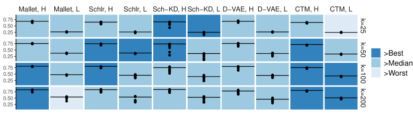
To evaluate this method, we compare the alignment score of the ensemble (§2.4.2) combining the runs, versus the alignment score of each individual member run. We do so across each of the 400 contexts (model, dataset, , high versus low label granularity, and metric). Figure 1 illustrates a summary of results for the purity alignment metric on the Wikipedia dataset. Across the full range of our experimentation, the ensemble improves on the median member in 97% of all the contexts, and it is always better than the worst member (full results in Appendix A.5).
7 Conclusions
A tool can be considered broken when it doesn’t work well for its intended use. In this paper we have focused on a widespread use case for topic models, their application in text content analysis; we have carefully motivated criteria for measuring the extent to which a topic model is serving those needs; and we have demonstrated through comprehensive and replicable experimentation that, when measured on those criteria, recent and representative neural topic models fail to improve on the classical implementation of LDA in Mallet. In particular, Mallet is much more stable, reducing concerns from the content analysis perspective that different runs could yield very different codesets. Equally important, across the vast majority of contexts, its discovered categories are reliable as measured via alignment with ground-truth human categories. For people seeking to use topic modeling in content analysis, therefore, Mallet may still be the best available tool for the job.
That said, there are still good reasons to investigate neural topic models. Foremost among these is the fact that they can benefit from pretraining on vast, general samples of language (e.g. Hoyle et al., 2020; Bianchi et al., 2021a; Feng et al., 2022). Neural realizations of topic models can also be integrated smoothly for joint modeling within larger neural architectures (e.g. Lau et al., 2017; Wang et al., 2019, 2020), and hold the promise of being more straightforward to use multilingually (e.g. Wu et al., 2020; Bianchi et al., 2021b; Mueller and Dredze, 2021) or multimodally (e.g. Zheng et al., 2015).141414See Zhao et al. (2021) for more potential advantages of neural topic modeling. We therefore introduced one possible way to address the shortcomings we identified using a straightforward ensemble technique.
Perhaps the most important take-away we would suggest is that development of new topic models—indeed, of all NLP models—should be done with use cases firmly in mind. Some models are enabling technologies, without a direct user-facing purpose, and others are intended to produce results directly for human consumption. But whatever the goal, the driving question for methodological development and evaluation should not be how to demonstrate an improvement in “state of the art”, it should be why the model is being created in the first place and what measurements will demonstrate improved performance for that intended purpose.
Limitations
Our studies used only English datasets, while topic modeling has been used to characterize texts in many languages. While theoretically we see no reason why our results and findings should not generalize beyond the English language, empirical generalizability across languages remains to be determined.
Our method for measuring alignment of model-induced categories with human-determined categories relies on ground-truth human labels, potentially limiting its broader applicability. In addition, the categories in the Wikipedia data were not, to our knowledge, produced via a traditional human content analysis process. We are currently designing a follow-up study in which human subject matter experts perform traditional content analysis from scratch on the same dataset used for topic modeling, in order to provide a head-to-head comparison between automated and traditional methods and to establish human upper bounds on inter-coder reliability.
Our literature review of topic modeling use cases was not a formal systematic review (Moher et al., 2009). It relied on Semantic Scholar’s content and its discipline categorization, and potentially excluded papers in computer science that were about the use of topic models rather than method development. It seems clear that text content analysis a dominant use case for topic modeling, if not the dominant use case. In the social sciences, we also note frequent use of the Structural Topic Model Roberts et al. (2014) which, like Scholar, can incorporate metadata into model estimation—we leave an evaluation of this use case to future work.
8 Acknowledgements
This material is based upon work supported in part by the National Science Foundation under Grants 2031736 and 2008761 and by Amazon. We thank David Mimno and Xanda Schofield for their input on earlier drafts, as well as our anonymous reviewers for their helpful comments.
References
- Agrawal et al. (2018) Amritanshu Agrawal, Wei Fu, and Tim Menzies. 2018. What is wrong with topic modeling? and how to fix it using search-based software engineering. Information and Software Technology, 98:74–88.
- Almquist and Bagozzi (2019) Zack W. Almquist and Benjamin E. Bagozzi. 2019. Using radical environmentalist texts to uncover network structure and network features. Sociological Methods & Research, 48:905 – 960.
- Amozegar (2021) Mahdiyeh Amozegar. 2021. Tweeting in Times of Crisis: Shifting Personal Value Priorities in Corporate Communications and Impact on Consumer Engagement. Ph.D. thesis, Université d’Ottawa/University of Ottawa.
- Aniss et al. (2021) Qostal Aniss, Moumen Aniss, and Lakhrissi Younes. 2021. The role of social networks in personality analysis for recruitment of laureates: A systematic review and exploratory study. SHS Web of Conferences.
- Artstein and Poesio (2008) Ron Artstein and Massimo Poesio. 2008. Survey article: Inter-coder agreement for computational linguistics. Computational Linguistics, 34(4):555–596.
- Ballester and Penner (2022) Omar Ballester and Orion Penner. 2022. Robustness, replicability and scalability in topic modelling. Journal of Informetrics, 16(1):101224.
- Bateman et al. (2019) Tyler Bateman, Shyon Baumann, and Josée Johnston. 2019. Meat as benign, meat as risk: Mapping news discourse of an ambiguous issue. Poetics.
- Bayard de Volo et al. (2020) Theo Bayard de Volo, Alfredo Gomez, Tatsuki Kuze, and Alexandra Schofield. 2020. LDA in the wild: How practitioners develop topic models. In West Coast NLP.
- Bell and Scott (2020) Emily Bell and Tyler A. Scott. 2020. Common institutional design, divergent results: A comparative case study of collaborative governance platforms for regional water planning. Environmental Science & Policy, 111:63–73.
- Bianchi et al. (2021a) Federico Bianchi, Silvia Terragni, and Dirk Hovy. 2021a. Pre-training is a hot topic: Contextualized document embeddings improve topic coherence. In Proceedings of the 59th Annual Meeting of the Association for Computational Linguistics and the 11th International Joint Conference on Natural Language Processing (Volume 2: Short Papers), pages 759–766, Online. Association for Computational Linguistics.
- Bianchi et al. (2021b) Federico Bianchi, Silvia Terragni, Dirk Hovy, Debora Nozza, and Elisabetta Fersini. 2021b. Cross-lingual contextualized topic models with zero-shot learning. In Proceedings of the 16th Conference of the European Chapter of the Association for Computational Linguistics: Main Volume, pages 1676–1683, Online. Association for Computational Linguistics.
- Blei and Lafferty (2006) David Blei and John Lafferty. 2006. Correlated topic models. Advances in neural information processing systems, 18:147.
- Blei et al. (2003) David M Blei, Andrew Y Ng, and Michael I Jordan. 2003. Latent dirichlet allocation. Journal of machine Learning research, 3(Jan):993–1022.
- Boyd-Graber et al. (2014) Jordan Boyd-Graber, David Mimno, and David Newman. 2014. Care and feeding of topic models: Problems, diagnostics, and improvements. Handbook of mixed membership models and their applications, 225255.
- Burkhardt and Kramer (2019) Sophie Burkhardt and Stefan Kramer. 2019. Decoupling Sparsity and Smoothness in the Dirichlet Variational Autoencoder Topic Model.
- Card et al. (2018) Dallas Card, Chenhao Tan, and Noah A. Smith. 2018. Neural models for documents with metadata. In Proceedings of the 56th Annual Meeting of the Association for Computational Linguistics (Volume 1: Long Papers), pages 2031–2040, Melbourne, Australia. Association for Computational Linguistics.
- Chang et al. (2009) Jonathan Chang, Sean Gerrish, Chong Wang, Jordan L. Boyd-graber, and David M. Blei. 2009. Reading Tea Leaves: How Humans Interpret Topic Models. In Advances in Neural Information Processing Systems 22, pages 288–296. Curran Associates, Inc.
- Chuang et al. (2013) Jason Chuang, Sonal Gupta, Christopher Manning, and Jeffrey Heer. 2013. Topic model diagnostics: Assessing domain relevance via topical alignment. In International conference on machine learning, pages 612–620. PMLR.
- Chuang et al. (2015) Jason Chuang, Margaret E. Roberts, Brandon M. Stewart, Rebecca Weiss, Dustin Tingley, Justin Grimmer, and Jeffrey Heer. 2015. TopicCheck: Interactive alignment for assessing topic model stability. In Proceedings of the 2015 Conference of the North American Chapter of the Association for Computational Linguistics: Human Language Technologies, pages 175–184, Denver, Colorado. Association for Computational Linguistics.
- Coco et al. (2020) Alberto Coco, Nicola Viegi, et al. 2020. The monetary policy of the South African Reserve Bank: Stance, communication and credibility. Economic Research and Statistics Department, South African Reserve Bank.
- Crouse (2016) David F. Crouse. 2016. On implementing 2d rectangular assignment algorithms. IEEE Transactions on Aerospace and Electronic Systems, 52(4):1679–1696.
- Das et al. (2020) Dipok Chandra Das, Dipa Rani Saha, T Kabir, Prosanto Deb, and Joyjeet Bhowmik. 2020. Analysis of covid-19 coverage in bangladesh news media using topic modelling.
- Day and Edelsbrunner (1984) William HE Day and Herbert Edelsbrunner. 1984. Efficient algorithms for agglomerative hierarchical clustering methods. Journal of classification, 1(1):7–24.
- Dieng et al. (2020) Adji B Dieng, Francisco JR Ruiz, and David M Blei. 2020. Topic modeling in embedding spaces. Transactions of the Association for Computational Linguistics, 8:439–453.
- Doogan (2022) Caitlin Doogan. 2022. A Topic is Not a Theme: Towards a Contextualised Approach to Topic Modelling. Ph.D. thesis, Monash University.
- Doogan and Buntine (2021) Caitlin Doogan and Wray Buntine. 2021. Topic model or topic twaddle? re-evaluating semantic interpretability measures. In Proceedings of the 2021 Conference of the North American Chapter of the Association for Computational Linguistics: Human Language Technologies, pages 3824–3848, Online. Association for Computational Linguistics.
- dos Santos et al. (2019) Tiago Ribeiro dos Santos, Jorge Louçã, and Hélder Coelho. 2019. The digital transformation of the public sphere. Systems Research and Behavioral Science.
- Dybowski et al. (2019) T Philipp Dybowski, Bernd Kempa, et al. 2019. The ecb’s monetary pillar after the financial crisis. Center for Quantitative Economics Working Papers, (8519).
- Eom et al. (2021) Han-Sung Eom, Sungyun Choi, and Sang Ok Choi. 2021. Marketable value estimation of patents using ensemble learning methodology: Focusing on u.s. patents for the electricity sector. PLoS ONE, 16.
- Feng et al. (2022) Jiachun Feng, Zusheng Zhang, Cheng Ding, Yanghui Rao, Haoran Xie, and Fu Lee Wang. 2022. Context reinforced neural topic modeling over short texts. Information Sciences.
- Fernandez et al. (2021) Raul Fernandez, Brenda Palma Guizar, and Caterina Rho. 2021. A sentiment-based risk indicator for the mexican financial sector. Latin American Journal of Central Banking, 2(3):100036.
- Fung et al. (2021) Anthony A. Fung, Andy Zhou, Jennifer K. Vanos, and Geert W. Schmid-Schönbein. 2021. Enhanced intestinal permeability and intestinal co-morbidities in heat strain: A review and case for autodigestion. Temperature: Multidisciplinary Biomedical Journal, 8:223 – 244.
- Gao et al. (2021) Shuang Gao, Shivani Pandya, Smisha Agarwal, and João Sedoc. 2021. Topic modeling for maternal health using Reddit. In Proceedings of the 12th International Workshop on Health Text Mining and Information Analysis, pages 69–76, online. Association for Computational Linguistics.
- Goldberg (2020) Yoav Goldberg. 2020. Tweet from @yoavgo on 2020-12-19.
- Greene et al. (2014) Derek Greene, Derek O?Callaghan, and Pádraig Cunningham. 2014. How many topics? stability analysis for topic models. In Joint European conference on machine learning and knowledge discovery in databases, pages 498–513. Springer.
- Griffiths (2002) Tom Griffiths. 2002. Gibbs sampling in the generative model of latent dirichlet allocation. 518.
- Grimmer and Stewart (2013) Justin Grimmer and Brandon M Stewart. 2013. Text as data: The promise and pitfalls of automatic content analysis methods for political texts. Political analysis, 21(3):267–297.
- Gupta et al. (2020) Itika Gupta, Barbara Di Eugenio, Devika Salunke, Andrew Boyd, Paula Allen-Meares, Carolyn Dickens, and Olga Garcia. 2020. Heart failure education of African American and Hispanic/Latino patients: Data collection and analysis. In Proceedings of the First Workshop on Natural Language Processing for Medical Conversations, pages 41–46, Online. Association for Computational Linguistics.
- Harrando et al. (2021) Ismail Harrando, Pasquale Lisena, and Raphael Troncy. 2021. Apples to apples: A systematic evaluation of topic models. In Proceedings of the International Conference on Recent Advances in Natural Language Processing (RANLP 2021), pages 483–493, Held Online. INCOMA Ltd.
- He et al. (2022) Jinbo He, Jingshi Kang, Shaojing Sun, Marita Cooper, Hana F Zickgraf, and Yujia Zhai. 2022. The landscape of eating disorders research: A 40-year bibliometric analysis. European eating disorders review : the journal of the Eating Disorders Association.
- Hopkins et al. (2020) Daniel J. Hopkins, Eric Schickler, and David Azizi. 2020. From many divides, one? the polarization and nationalization of american state party platforms, 1918-2017. Social Science Research Network.
- Hou et al. (2021) Keke Hou, Tingting Hou, and Lili Cai. 2021. Public attention about covid-19 on social media: An investigation based on data mining and text analysis. Personality and Individual Differences, 175:110701 – 110701.
- Hoyle et al. (2021) Alexander Hoyle, Pranav Goel, Andrew Hian-Cheong, Denis Peskov, Jordan Boyd-Graber, and Philip Resnik. 2021. Is automated topic model evaluation broken? the incoherence of coherence. In Advances in Neural Information Processing Systems, volume 34, pages 2018–2033. Curran Associates, Inc.
- Hoyle et al. (2020) Alexander Miserlis Hoyle, Pranav Goel, and Philip Resnik. 2020. Improving Neural Topic Models using Knowledge Distillation. In Proceedings of the 2020 Conference on Empirical Methods in Natural Language Processing (EMNLP), pages 1752–1771, Online. Association for Computational Linguistics.
- Hu et al. (2021) Tao Hu, Siqin Wang, Wei Luo, Mengxi Zhang, Xiao Huang, Yingwei Yan, Regina Liu, Kelly Ly, Viraj Kacker, Bing She, and Zhenlong Li. 2021. Revealing public opinion towards covid-19 vaccines with twitter data in the united states: Spatiotemporal perspective. Journal of Medical Internet Research, 23.
- Jang et al. (2021) Hyeju Jang, Emily S. Rempel, David Roth, Giuseppe Carenini, and Naveed Zafar Janjua. 2021. Tracking covid-19 discourse on twitter in north america: Infodemiology study using topic modeling and aspect-based sentiment analysis. Journal of Medical Internet Research, 23.
- Jing et al. (2021) Min Jing, Raymond R. Bond, Louise J Robertson, Julie Moore, Amanda M Kowalczyk, Ruth K Price, William P Burns, M. Andrew Nesbit, James Mclaughlin, and Tara Moore. 2021. User experience analysis of abc-19 rapid test via lateral flow immunoassays for self-administrated sars-cov-2 antibody testing. Scientific Reports, 11.
- Johnson et al. (2022) Amy K Johnson, Runa Bhaumik, Debarghya Nandi, Abhishikta Roy, and Supriya D Mehta. 2022. Is this herpes or syphilis?: Latent dirichlet allocation analysis of sexually transmitted disease-related reddit posts during the covid-19 pandemic. medRxiv.
- Kaufman and Rousseeuw (2008) Leonard Kaufman and Peter J. Rousseeuw. 2008. Partitioning Around Medoids (Program PAM), pages 68–125. John Wiley & Sons, Inc.
- Kingma and Welling (2014) Diederik P. Kingma and Max Welling. 2014. Auto-Encoding Variational Bayes. In 2nd International Conference on Learning Representations, ICLR 2014, Banff, AB, Canada, April 14-16, 2014, Conference Track Proceedings.
- Ko et al. (2021) Kilkon Ko, Hyun Hee Park, Dong Chul Shim, and Kyungdong Kim. 2021. The change of administrative capacity in korea: contemporary trends and lessons. International Review of Administrative Sciences, 87:238 – 255.
- Koltcov et al. (2014) Sergei Koltcov, Olessia Koltsova, and Sergey Nikolenko. 2014. Latent dirichlet allocation: stability and applications to studies of user-generated content. In Proceedings of the 2014 ACM conference on Web science, pages 161–165.
- Korenčić et al. (2021) Damir Korenčić, Strahil Ristov, Jelena Repar, and Jan Šnajder. 2021. A topic coverage approach to evaluation of topic models. IEEE Access, 9:123280–123312.
- Krippendorff (2018) Klaus Krippendorff. 2018. Content analysis: An introduction to its methodology. Sage publications.
- kyu Park et al. (2020) Hyun kyu Park, Robert Phaal, Jae-Yun Ho, and Eoin O’Sullivan. 2020. Twenty years of technology and strategic roadmapping research: A school of thought perspective. Technological Forecasting and Social Change, 154:119965.
- Lattimer et al. (2022) Tahleen A. Lattimer, Kelly E. Tenzek, Yotam Ophir, and Suzanne S. Sullivan. 2022. Exploring web-based twitter conversations surrounding national healthcare decisions day and advance care planning from a sociocultural perspective: Computational mixed methods analysis. JMIR Formative Research, 6.
- Lau et al. (2017) Jey Han Lau, Timothy Baldwin, and Trevor Cohn. 2017. Topically driven neural language model. In Proceedings of the 55th Annual Meeting of the Association for Computational Linguistics (Volume 1: Long Papers), pages 355–365, Vancouver, Canada. Association for Computational Linguistics.
- Lau et al. (2014) Jey Han Lau, David Newman, and Timothy Baldwin. 2014. Machine reading tea leaves: Automatically evaluating topic coherence and topic model quality. In Proceedings of the 14th Conference of the European Chapter of the Association for Computational Linguistics, pages 530–539, Gothenburg, Sweden. Association for Computational Linguistics.
- Lee et al. (2021a) Junho Lee, Ikjun Kim, Hyomin Kim, and Juyoung Kang. 2021a. Swot-ahp analysis of the korean satellite and space industry: Strategy recommendations for development. Technological Forecasting and Social Change.
- Lee and Hong (2020) Sae-Mi Lee and Soongoo Hong. 2020. Policy agenda proposals from text mining analysis of patents and news articles. Journal of Digital Convergence, 18:1–12.
- Lee et al. (2021b) Yoon Kyung Lee, Yoonwon Jung, Inju Lee, Jae Eun Park, and Sowon Hahn. 2021b. Building a psychological ground truth dataset with empathy and theory-of-mind during the covid-19 pandemic. In Proceedings of the Annual Meeting of the Cognitive Science Society, volume 43.
- Li et al. (2021) Kai Li, Xing Liu, Feng Mai, and Tengfei Zhang. 2021. The role of corporate culture in bad times: Evidence from the covid-19 pandemic. Journal of Financial and Quantitative Analysis, 56:2545 – 2583.
- Liberati et al. (2009) Alessandro Liberati, Douglas G Altman, Jennifer Tetzlaff, Cynthia Mulrow, Peter C Gøtzsche, John PA Ioannidis, Mike Clarke, Philip J Devereaux, Jos Kleijnen, and David Moher. 2009. The PRISMA statement for reporting systematic reviews and meta-analyses of studies that evaluate health care interventions: explanation and elaboration. Journal of clinical epidemiology, 62(10):e1–e34.
- Lloyd (1957) SP Lloyd. 1957. Least square quantization in pcm. bell telephone laboratories paper. published in journal much later: Lloyd, sp: Least squares quantization in pcm. IEEE Trans. Inform. Theor.(1957/1982), 18:5.
- Madzík and Falat (2022) Peter Madzík and Lukas Falat. 2022. State-of-the-art on analytic hierarchy process in the last 40 years: Literature review based on latent dirichlet allocation topic modelling. PLoS ONE, 17.
- Mamaysky (2020) Harry Mamaysky. 2020. News and markets in the time of covid-19. Econometric Modeling: Capital Markets - Asset Pricing eJournal.
- Mantyla et al. (2018) Mika V Mantyla, Maelick Claes, and Umar Farooq. 2018. Measuring LDA topic stability from clusters of replicated runs. In Proceedings of the 12th ACM/IEEE international symposium on empirical software engineering and measurement, pages 1–4.
- Markides et al. (2022) Brittany R Markides, Rachel Laws, Kylie D. Hesketh, Ralph Maddison, Elizabeth A Denney-Wilson, and Karen Jane Campbell. 2022. A thematic cluster analysis of parents’ online discussions about fussy eating. Maternal & Child Nutrition, 18.
- Marshall (2021) Pablo Marshall. 2021. Contribution of open-ended questions in student evaluation of teaching. Higher Education Research & Development.
- McCallum (2002) Andrew Kachites McCallum. 2002. Machine learning with MALLET. http://mallet.cs.umass.edu.
- Merity et al. (2017) Stephen Merity, Caiming Xiong, James Bradbury, and Richard Socher. 2017. Pointer Sentinel Mixture Models. ICLR.
- Miller (2019) Daniel Taninecz Miller. 2019. Three International Studies Computational Social Science Inquiries Examining Large Corpora of Natural Data. Ph.D. thesis.
- Miller and McCoy (2017) John Miller and Kathleen McCoy. 2017. Topic model stability for hierarchical summarization. In Proceedings of the Workshop on New Frontiers in Summarization, pages 64–73, Copenhagen, Denmark. Association for Computational Linguistics.
- Mimno (2022) David Mimno. 2022. Why I don’t recommend stochastic variational Bayes for topic models. Blog post. Accessed October 24, 2022.
- Mitchell (2020) Andrew Mitchell. 2020. Mode-2 knowledge production within community-based sustainability projects: Applying textual and thematic analytics to action research conversations. Administrative Sciences, 10:90.
- Moher et al. (2009) David Moher, Alessandro Liberati, Jennifer Tetzlaff, Douglas G Altman, and PRISMA Group. 2009. Preferred reporting items for systematic reviews and meta-analyses: the PRISMA statement. Annals of internal medicine, 151(4):264–269.
- Mueller and Dredze (2021) Aaron Mueller and Mark Dredze. 2021. Fine-tuning encoders for improved monolingual and zero-shot polylingual neural topic modeling. In Proceedings of the 2021 Conference of the North American Chapter of the Association for Computational Linguistics: Human Language Technologies, pages 3054–3068, Online. Association for Computational Linguistics.
- Neresini et al. (2019) Federico Neresini, Paolo Giardullo, Emanuele Di Buccio, and Alberto Cammozzo. 2019. Exploring socio-technical future scenarios in the media: the energy transition case in italian daily newspapers. Quality & Quantity, 54:147–168.
- Newman et al. (2010) David Newman, Jey Han Lau, Karl Grieser, and Timothy Baldwin. 2010. Automatic evaluation of topic coherence. In Human Language Technologies: The 2010 Annual Conference of the North American Chapter of the Association for Computational Linguistics, pages 100–108, Los Angeles, California. Association for Computational Linguistics.
- Ng and Indran (2021) Reuben Ng and Nicole Indran. 2021. Role-based framing of older adults linked to decreased ageism over 210 years: Evidence from a 600-million-word historical corpus. The Gerontologist, 62:589 – 597.
- Ning et al. (2020) Li Ning, Peng Lifang, and He Huixin. 2020. Prediction correction topic evolution research for metabolic pathways of the gut microbiota. Frontiers in Molecular Biosciences, 7.
- Noble et al. (2021) Peter-John Mäntylä Noble, Charlotte Appleton, Alan D. Radford, and Goran Nenadic. 2021. Using topic modelling for unsupervised annotation of electronic health records to identify an outbreak of disease in uk dogs. PLoS ONE, 16.
- Pedregosa et al. (2011) Fabian Pedregosa, Gaël Varoquaux, Alexandre Gramfort, Vincent Michel, Bertrand Thirion, Olivier Grisel, Mathieu Blondel, Peter Prettenhofer, Ron Weiss, Vincent Dubourg, et al. 2011. Scikit-learn: Machine learning in python. Journal of machine learning research, 12(Oct):2825–2830.
- Peterson and Hall (2020) Erik L. Peterson and Crystal L. Hall. 2020. "what is dead may not die": Locating marginalized concepts among ordinary biologists. Journal of the history of biology.
- Poursabzi-Sangdeh et al. (2016) Forough Poursabzi-Sangdeh, Jordan Boyd-Graber, Leah Findlater, and Kevin Seppi. 2016. ALTO: Active learning with topic overviews for speeding label induction and document labeling. In Proceedings of the 54th Annual Meeting of the Association for Computational Linguistics (Volume 1: Long Papers), pages 1158–1169, Berlin, Germany. Association for Computational Linguistics.
- Rand (1971) William M Rand. 1971. Objective criteria for the evaluation of clustering methods. Journal of the American Statistical association, 66(336):846–850.
- Reimers and Gurevych (2019) Nils Reimers and Iryna Gurevych. 2019. Sentence-BERT: Sentence embeddings using Siamese BERT-networks. In Proceedings of the 2019 Conference on Empirical Methods in Natural Language Processing and the 9th International Joint Conference on Natural Language Processing (EMNLP-IJCNLP), pages 3982–3992, Hong Kong, China. Association for Computational Linguistics.
- Roberts et al. (2013) Margaret E Roberts, Brandon M Stewart, Dustin Tingley, Edoardo M Airoldi, et al. 2013. The structural topic model and applied social science. In Advances in neural information processing systems workshop on topic models: computation, application, and evaluation, volume 4, pages 1–20. Harrahs and Harveys, Lake Tahoe.
- Roberts et al. (2014) Margaret E Roberts, Brandon M Stewart, Dustin Tingley, Christopher Lucas, Jetson Leder-Luis, Shana Kushner Gadarian, Bethany Albertson, and David G Rand. 2014. Structural topic models for open-ended survey responses. American journal of political science, 58(4):1064–1082.
- Rubio (2005) Doris McGartland Rubio. 2005. Content validity. Elsevier.
- Scarborough and Crabbe (2021) William J. Scarborough and Rowena Crabbe. 2021. Place brands across u.s. cities and growth in local high-technology sectors. Journal of Business Research, 130:70–85.
- Schreier (2012) Margrit Schreier. 2012. Qualitative content analysis in practice. Sage publications.
- Shapiro and Markoff (1997) G Shapiro and J Markoff. 1997. A Matter of Definition. Mahwah: Lawrence Erlbaum Assoc.
- Shin et al. (2019) Jinnie Shin, Qi Guo, and Mark Gierl. 2019. Multiple-choice item distractor development using topic modeling approaches. Frontiers in Psychology, 10.
- Smith (2000) Charles P Smith. 2000. Content analysis and narrative analysis. Handbook of research methods in social and personality psychology, 2000:313–335.
- Squires et al. (2022) Allison Patricia Squires, Maya N. Clark-Cutaia, Marcus D. Henderson, Gavin Arneson, and Philip Resnik. 2022. “should i stay or should i go?” nurses’ perspectives about working during the covid-19 pandemic’s first wave in the united states: A summative content analysis combined with topic modeling. International Journal of Nursing Studies, 131:104256 – 104256.
- Steinley (2004) Douglas Steinley. 2004. Properties of the hubert-arabie adjusted rand index. Psychological methods, 9:386–96.
- Stemler (2000) Steve Stemler. 2000. An overview of content analysis. Practical assessment, research, and evaluation, 7(1):17.
- Strehl and Ghosh (2002) Alexander Strehl and Joydeep Ghosh. 2002. Cluster ensembles - a knowledge reuse framework for combining multiple partitions. Journal of Machine Learning Research, 3:583–617.
- Viñán-Ludeña and de Campos (2021) Marlon Santiago Viñán-Ludeña and Luis M de Campos. 2021. Analyzing tourist data on twitter: a case study in the province of granada at spain. Journal of Hospitality and Tourism Insights.
- Virtanen (2021) Seppo Virtanen. 2021. Uncovering dynamic textual topics that explain crime. Royal Society Open Science, 8.
- Wang et al. (2021) Chihuangji Wang, Edward S. Steinfeld, Jordana L. Maisel, and Bumjoon Kang. 2021. Is your smart city inclusive? evaluating proposals from the u.s. department of transportation’s smart city challenge. Sustainable Cities and Society, 74:103148.
- Wang et al. (2019) Wenlin Wang, Zhe Gan, Hongteng Xu, Ruiyi Zhang, Guoyin Wang, Dinghan Shen, Changyou Chen, and Lawrence Carin. 2019. Topic-guided variational auto-encoder for text generation. In Proceedings of the 2019 Conference of the North American Chapter of the Association for Computational Linguistics: Human Language Technologies, Volume 1 (Long and Short Papers), pages 166–177, Minneapolis, Minnesota. Association for Computational Linguistics.
- Wang et al. (2020) Zhengjue Wang, Zhibin Duan, Hao Zhang, Chaojie Wang, Long Tian, Bo Chen, and Mingyuan Zhou. 2020. Friendly topic assistant for transformer based abstractive summarization. In Proceedings of the 2020 Conference on Empirical Methods in Natural Language Processing (EMNLP), pages 485–497, Online. Association for Computational Linguistics.
- Webber et al. (2010) William Webber, Alistair Moffat, and Justin Zobel. 2010. A similarity measure for indefinite rankings. ACM Transactions on Information Systems (TOIS), 28(4):1–38.
- Weber (1990) Robert Philip Weber. 1990. Basic content analysis, volume 49. Sage.
- Wehrheim et al. (2021) Lino Wehrheim, Tobias Alexander Jopp, and Mark Spoerer. 2021. Turn, turn, turn: A digital history of german historiography, 1950-2019. Technical report, Working Papers of the Priority Programme 1859" Experience and Expectation ….
- Wu et al. (2020) Xiaobao Wu, Chunping Li, Yan Zhu, and Yishu Miao. 2020. Learning multilingual topics with neural variational inference. In CCF International Conference on Natural Language Processing and Chinese Computing, pages 840–851. Springer.
- Yamada and Inoue (2019) Taizo Yamada and Satoshi Inoue. 2019. Detection and time series variation of latent topic from diary in northern and southern courts period of japan. 2019 Pacific Neighborhood Consortium Annual Conference and Joint Meetings (PNC), pages 1–8.
- Yang and Fang (2021) Tian Yang and Kecheng Fang. 2021. How dark corners collude: a study on an online chinese alt-right community. Information, Communication & Society.
- Ye et al. (2020) Qian Ye, Xiaohong Chen, Kaan Ozbay, and Yonggang Wang. 2020. How people view and respond to special events in shared mobility: Case study of two didi safety incidents via sina weibo. In 20th COTA International Conference of Transportation Professionals: Advanced Transportation Technologies and Development-Enhancing Connections, CICTP 2020, pages 3229–3240. American Society of Civil Engineers (ASCE).
- Yuan et al. (2020) Faxi Yuan, Min Li, and Rui Liu. 2020. Understanding the evolutions of public responses using social media: Hurricane matthew case study. International journal of disaster risk reduction, 51:101798.
- Zhang et al. (2021) Yipeng Zhang, Hanjia Lyu, Yubao Liu, Xiyang Zhang, Yu Wang, and Jiebo Luo. 2021. Monitoring depression trends on twitter during the covid-19 pandemic: Observational study. JMIR Infodemiology, 1.
- Zhao et al. (2021) He Zhao, Dinh Phung, Viet Huynh, Yuan Jin, Lan Du, and Wray Buntine. 2021. Topic modelling meets deep neural networks: A survey. In Proceedings of the Thirtieth International Joint Conference on Artificial Intelligence, IJCAI-21, pages 4713–4720. International Joint Conferences on Artificial Intelligence Organization. Survey Track.
- Zhao and Karypis (2002) Ying Zhao and George Karypis. 2002. Criterion functions for document clustering: Experiments and analysis.
- Zheng et al. (2015) Yin Zheng, Yu-Jin Zhang, and Hugo Larochelle. 2015. A deep and autoregressive approach for topic modeling of multimodal data. IEEE transactions on pattern analysis and machine intelligence, 38(6):1056–1069.
Appendix A Appendix
| 5k | 15k | ||||||||||||||||
|---|---|---|---|---|---|---|---|---|---|---|---|---|---|---|---|---|---|
| 25 | 50 | 100 | 200 | 25 | 50 | 100 | 200 | ||||||||||
| B | B | B | B | B | B | B | B | ||||||||||
| Bills | Mallet | 0.76 | 0.26 | 0.75 | 0.29 | 0.73 | 0.30 | 0.70 | 0.36 | 0.73 | 0.26 | 0.74 | 0.30 | 0.72 | 0.34 | 0.70 | 0.37 |
| Scholar | 0.72 | 0.42 | 0.67 | 0.39 | 0.67 | 0.38 | 0.68 | 0.38 | 0.78 | 0.52 | 0.73 | 0.47 | 0.70 | 0.44 | 0.71 | 0.43 | |
| Schlr+KD | 0.84 | 0.43 | 0.78 | 0.38 | 0.70 | 0.31 | 0.69 | 0.29 | 0.83 | 0.46 | 0.80 | 0.38 | 0.74 | 0.31 | 0.72 | 0.29 | |
| d-vae | 0.91 | 0.34 | 0.86 | 0.54 | 0.85 | 0.68 | 0.74 | 0.81 | 0.95 | 0.40 | 0.90 | 0.57 | 0.90 | 0.71 | 0.91 | 0.79 | |
| ctm | 0.78 | 0.43 | 0.77 | 0.47 | 0.73 | 0.51 | 0.70 | 0.52 | 0.80 | 0.44 | 0.81 | 0.53 | 0.79 | 0.60 | 0.73 | 0.62 | |
| Wiki | Mallet | 0.70 | 0.22 | 0.60 | 0.26 | 0.56 | 0.28 | 0.54 | 0.31 | 0.69 | 0.26 | 0.62 | 0.29 | 0.55 | 0.29 | 0.50 | 0.31 |
| Scholar | 0.77 | 0.39 | 0.66 | 0.31 | 0.62 | 0.33 | 0.59 | 0.32 | 0.75 | 0.45 | 0.69 | 0.38 | 0.65 | 0.38 | 0.60 | 0.37 | |
| Schlr+KD | 0.77 | 0.41 | 0.66 | 0.33 | 0.62 | 0.33 | 0.53 | 0.28 | 0.78 | 0.52 | 0.70 | 0.44 | 0.62 | 0.38 | 0.54 | 0.34 | |
| d-vae | 0.93 | 0.24 | 0.88 | 0.25 | 0.83 | 0.26 | 0.82 | 0.29 | 0.95 | 0.28 | 0.90 | 0.30 | 0.83 | 0.32 | 0.78 | 0.33 | |
| ctm | 0.75 | 0.39 | 0.73 | 0.39 | 0.72 | 0.45 | 0.70 | 0.51 | 0.77 | 0.42 | 0.74 | 0.41 | 0.75 | 0.51 | 0.73 | 0.57 | |
| 25 | 50 | 100 | 200 | ||||||||||
|---|---|---|---|---|---|---|---|---|---|---|---|---|---|
| ARI | NMI | ARI | NMI | ARI | NMI | ARI | NMI | ||||||
| Bills | Mallet | 0.30 | 0.46 | 0.47 | 0.35 | 0.49 | 0.48 | 0.34 | 0.51 | 0.45 | 0.22 | 0.51 | 0.37 |
| Scholar | 0.25 | 0.45 | 0.42 | 0.25 | 0.48 | 0.43 | 0.21 | 0.51 | 0.40 | 0.15 | 0.52 | 0.34 | |
| Schlr+KD | 0.24 | 0.42 | 0.40 | 0.23 | 0.46 | 0.43 | 0.20 | 0.49 | 0.40 | 0.13 | 0.49 | 0.34 | |
| d-vae | 0.26 | 0.45 | 0.45 | 0.21 | 0.45 | 0.45 | 0.10 | 0.43 | 0.42 | 0.04 | 0.39 | 0.41 | |
| ctm | 0.23 | 0.40 | 0.39 | 0.27 | 0.46 | 0.43 | 0.24 | 0.48 | 0.40 | 0.18 | 0.49 | 0.34 | |
| Wiki | Mallet | 0.23 | 0.65 | 0.41 | 0.32 | 0.70 | 0.50 | 0.39 | 0.73 | 0.56 | 0.39 | 0.74 | 0.56 |
| Scholar | 0.22 | 0.62 | 0.39 | 0.33 | 0.68 | 0.49 | 0.39 | 0.72 | 0.54 | 0.38 | 0.74 | 0.54 | |
| Schlr+KD | 0.20 | 0.61 | 0.37 | 0.30 | 0.67 | 0.47 | 0.39 | 0.71 | 0.53 | 0.39 | 0.74 | 0.54 | |
| d-vae | 0.24 | 0.66 | 0.41 | 0.32 | 0.70 | 0.50 | 0.36 | 0.72 | 0.54 | 0.36 | 0.72 | 0.54 | |
| ctm | 0.21 | 0.60 | 0.36 | 0.28 | 0.65 | 0.44 | 0.32 | 0.67 | 0.47 | 0.35 | 0.70 | 0.48 | |
| 25 | 50 | 100 | 200 | ||||||||||
|---|---|---|---|---|---|---|---|---|---|---|---|---|---|
| ARI | NMI | ARI | NMI | ARI | NMI | ARI | NMI | ||||||
| Bills | Mallet | 0.17 | 0.34 | 0.37 | 0.17 | 0.37 | 0.37 | 0.17 | 0.40 | 0.37 | 0.15 | 0.41 | 0.35 |
| Scholar | 0.06 | 0.18 | 0.22 | 0.09 | 0.27 | 0.26 | 0.07 | 0.27 | 0.23 | 0.05 | 0.26 | 0.19 | |
| Schlr+KD | 0.06 | 0.19 | 0.24 | 0.07 | 0.25 | 0.27 | 0.06 | 0.27 | 0.26 | 0.04 | 0.26 | 0.19 | |
| d-vae | 0.13 | 0.30 | 0.34 | 0.11 | 0.29 | 0.32 | 0.11 | 0.32 | 0.32 | 0.10 | 0.34 | 0.31 | |
| ctm | 0.11 | 0.28 | 0.31 | 0.12 | 0.32 | 0.31 | 0.10 | 0.35 | 0.29 | 0.08 | 0.37 | 0.26 | |
| Wiki | Mallet | 0.34 | 0.65 | 0.53 | 0.37 | 0.66 | 0.53 | 0.37 | 0.68 | 0.53 | 0.33 | 0.68 | 0.51 |
| Scholar | 0.29 | 0.61 | 0.48 | 0.32 | 0.64 | 0.51 | 0.30 | 0.63 | 0.47 | 0.24 | 0.61 | 0.41 | |
| Schlr+KD | 0.28 | 0.61 | 0.48 | 0.31 | 0.63 | 0.49 | 0.28 | 0.63 | 0.46 | 0.19 | 0.59 | 0.35 | |
| d-vae | 0.32 | 0.64 | 0.51 | 0.35 | 0.66 | 0.52 | 0.28 | 0.62 | 0.48 | 0.31 | 0.64 | 0.48 | |
| ctm | 0.32 | 0.61 | 0.49 | 0.32 | 0.63 | 0.48 | 0.29 | 0.64 | 0.46 | 0.27 | 0.65 | 0.45 | |
| 25 | 50 | 100 | 200 | ||||||||||
|---|---|---|---|---|---|---|---|---|---|---|---|---|---|
| ARI | NMI | ARI | NMI | ARI | NMI | ARI | NMI | ||||||
| Bills | Mallet | 0.17 | 0.34 | 0.37 | 0.17 | 0.37 | 0.38 | 0.17 | 0.40 | 0.38 | 0.15 | 0.42 | 0.36 |
| Scholar | 0.14 | 0.32 | 0.34 | 0.13 | 0.34 | 0.34 | 0.14 | 0.38 | 0.34 | 0.12 | 0.40 | 0.32 | |
| Schlr+KD | 0.10 | 0.27 | 0.31 | 0.09 | 0.29 | 0.32 | 0.08 | 0.33 | 0.30 | 0.06 | 0.32 | 0.31 | |
| d-vae | 0.11 | 0.27 | 0.32 | 0.05 | 0.26 | 0.31 | 0.03 | 0.25 | 0.32 | 0.01 | 0.21 | 0.34 | |
| ctm | 0.11 | 0.28 | 0.31 | 0.12 | 0.32 | 0.31 | 0.10 | 0.34 | 0.29 | 0.07 | 0.36 | 0.26 | |
| Wiki | Mallet | 0.33 | 0.65 | 0.52 | 0.37 | 0.66 | 0.54 | 0.38 | 0.68 | 0.54 | 0.34 | 0.69 | 0.52 |
| Scholar | 0.31 | 0.62 | 0.50 | 0.33 | 0.64 | 0.50 | 0.34 | 0.67 | 0.51 | 0.32 | 0.68 | 0.49 | |
| Schlr+KD | 0.30 | 0.63 | 0.49 | 0.38 | 0.67 | 0.54 | 0.37 | 0.69 | 0.52 | 0.34 | 0.70 | 0.51 | |
| d-vae | 0.34 | 0.65 | 0.52 | 0.37 | 0.67 | 0.54 | 0.36 | 0.67 | 0.52 | 0.32 | 0.66 | 0.49 | |
| ctm | 0.31 | 0.61 | 0.48 | 0.32 | 0.63 | 0.49 | 0.30 | 0.65 | 0.47 | 0.28 | 0.66 | 0.46 | |
A.1 Additional Results
Fixed Hyperparameters.
In tables 4 and 5, we report the equivalents of tables 2 and 3 when holding hyperparameters fixed, rather than letting them vary. We identify the hyperparameters for each model that achieve the highest average alignment metrics on across experimental contexts for one dataset, then use those hyperparameters to estimate models on the other dataset (hyperparameter values in section A.3). In this way, we follow a common paradigm in practical application of machine learning models: hyperparameters are determined based on an initial experimental context, then used in another. Broadly, Mallet is more stable and better-aligned than its neural counterparts in this setup, although the difference is not as stark as when hyperparameters are allowed to vary.
Held-out data.
In table 6, we report the alignment metrics for unseen category labels. To form the held-out data, we keep all high-level categories consistent between the training and held-out sets, but partition the low-level categories such that some are never seen during training (e.g., although documents from the high-level architecture category will be included in both splits, documents on bridges are only seen in training while those on lighthouses are held-out). Here too, Mallet generally has the highest alignment metrics over experimental contexts.
A.2 Details of LDA applications meta-analysis
| Coding Question | Answer | Count | ||||
|---|---|---|---|---|---|---|
|
Yes | 47 | (94%) | |||
|
|
33 | (70%) | |||
|
11 | (23%) | ||||
|
Yes | 32 | (64%) | |||
|
Yes | 34 | (68%) | |||
|
Yes | 27 | (54%) | |||
|
|
21 | (42%) | |||
|
9 | (18%) | ||||
|
7 | (14%) | ||||
|
7 | (14%) | ||||
|
4 | (8%) | ||||
|
2 | (4%) | ||||
|
2 | (4%) |
| Algo. | Worst | Med. | Best | |||
|---|---|---|---|---|---|---|
| Overall | -med. | RBO | 1.00 | 100% | 97% | 52% |
| Mallet | -med. | RBO | 1.00 | 100% | 98% | 55% |
| Scholar | -med. | Jcd. | 0.25 | 100% | 100% | 66% |
| Schlr+KD | Aggl. | RBO | 0.75 | 100% | 99% | 60% |
| d-vae | Aggl. | Jcd. | 0.25 | 100% | 92% | 29% |
| ctm | Aggl. | Jcd. | 0.25 | 100% | 100% | 90% |
Summary statistics of our meta-analysis of studies using LDA outside computer science are shown in Table 7. The major results were discussed in Section 2.2. We find that about half of the papers did not specify the exact LDA implementation they used in their study, which raises larger reproducibility concerns for scientific research. Note that one paper can be assigned multiple subject or fields of study by Semantic Scholar. All the papers used for the meta-analysis are shown in tables 9 and 10.
| Source |
|
|
|
|
|
|
||||||||||||||||||
|---|---|---|---|---|---|---|---|---|---|---|---|---|---|---|---|---|---|---|---|---|---|---|---|---|
| dos Santos et al. (2019) | Political Science | N | N/A | Y | N | N | ||||||||||||||||||
| Markides et al. (2022) | Medicine | Y | Both | Y | Y | Y | ||||||||||||||||||
| Miller (2019) | Political Science | Y | Both | N | N | Y | ||||||||||||||||||
| Scarborough and Crabbe (2021) | Business | Y | Topic-Word Only | Y | N | N | ||||||||||||||||||
| Jang et al. (2021) | Medicine | Y | Topic-Word Only | Y | Y | Y | ||||||||||||||||||
| Noble et al. (2021) | Medicine | Y | Topic-Word Only | Y | Y | Y | ||||||||||||||||||
| Yamada and Inoue (2019) | History | Y | Both | Y | N | Y | ||||||||||||||||||
| Zhang et al. (2021) | Medicine | Y | Topic-Word Only | Y | Y | N | ||||||||||||||||||
| Lee et al. (2021b) | Medicine | Y | Topic-Word Only | N | Y | N | ||||||||||||||||||
| Lattimer et al. (2022) | Medicine | Y | Both | Y | Y | N | ||||||||||||||||||
| Madzík and Falat (2022) | Medicine | Y | Topic-Word Only | Y | Y | Y | ||||||||||||||||||
| Wehrheim et al. (2021) | History | Y | Topic-Word Only | Y | Y | Y | ||||||||||||||||||
| Marshall (2021) | Psychology | Y | Topic-Word Only | N | Y | N | ||||||||||||||||||
| Hopkins et al. (2020) | Political Science | Y | Topic-Word Only | Y | Y | N | ||||||||||||||||||
| Ning et al. (2020) | Medicine | Y | Topic-Word Only | Y | Y | N | ||||||||||||||||||
| Aniss et al. (2021) | Psychology | Y | Topic-Word Only | N | Y | Y | ||||||||||||||||||
| Neresini et al. (2019) | Sociology | Y | Topic-Word Only | N | Y | N | ||||||||||||||||||
| Coco et al. (2020) | Economics | Y | Topic-Word Only | Y | N | N | ||||||||||||||||||
| Almquist and Bagozzi (2019) | Sociology | Y | Both | Y | Y | Y | ||||||||||||||||||
| Lee and Hong (2020) | Political Science | Y | Topic-Word Only | N | Y | Y | ||||||||||||||||||
| Li et al. (2021) | Business | Y | Both | Y | Y | Y | ||||||||||||||||||
| Hou et al. (2021) | Medicine | Y | Topic-Word Only | Y | Y | N | ||||||||||||||||||
| He et al. (2022) | Medicine | Y | Topic-Word Only | Y | Y | Y | ||||||||||||||||||
| Wang et al. (2021) | Business | Y | Topic-Word Only | N | N | Y | ||||||||||||||||||
| Dybowski et al. (2019) | Economics | Y | Both | Y | N | Y |
| Source |
|
|
|
|
|
|
||||||||||||||||||
|---|---|---|---|---|---|---|---|---|---|---|---|---|---|---|---|---|---|---|---|---|---|---|---|---|
| Gupta et al. (2020) | Psychology | Y | Topic-Word Only | N | Y | Y | ||||||||||||||||||
| Amozegar (2021) | Business | Y | Topic-Word Only | Y | Y | Y | ||||||||||||||||||
| Bell and Scott (2020) | Business | Y | Topic-Word Only | Y | N | N | ||||||||||||||||||
| Viñán-Ludeña and de Campos (2021) | Sociology | Y | Topic-Word Only | N | N | Y | ||||||||||||||||||
| Yang and Fang (2021) | Sociology | Y | Both | N | Y | N | ||||||||||||||||||
| Das et al. (2020) | Political Science | Y | Both | Y | Y | Y | ||||||||||||||||||
| Virtanen (2021) | Medicine | Y | Topic-Word Only | Y | Y | Y | ||||||||||||||||||
| Ye et al. (2020) | Sociology | Y | Topic-Word Only | Y | Y | N | ||||||||||||||||||
| Jing et al. (2021) | Medicine | Y | Topic-Word Only | N | N | N | ||||||||||||||||||
| Peterson and Hall (2020) | Medicine,Sociology | N | N/A | Y | N | Y | ||||||||||||||||||
| Ko et al. (2021) | Political Science | Y | Doc-Topic Only | Y | Y | N | ||||||||||||||||||
| Mitchell (2020) | Sociology | Y | Topic-Word Only | N | N | N | ||||||||||||||||||
| Fernandez et al. (2021) | Business | Y | Both | N | Y | N | ||||||||||||||||||
| Bateman et al. (2019) | Political Science | Y | Doc-Topic Only | Y | Y | Y | ||||||||||||||||||
| Fung et al. (2021) | Medicine | Y | Topic-Word Only | Y | Y | Y | ||||||||||||||||||
| Yuan et al. (2020) | Sociology | Y | Topic-Word Only | Y | Y | N | ||||||||||||||||||
| Eom et al. (2021) | Medicine | Y | Topic-Word Only | N | N | Y | ||||||||||||||||||
| Johnson et al. (2022) | Medicine | Y | Topic-Word Only | Y | Y | N | ||||||||||||||||||
| Squires et al. (2022) | Medicine | N | N/A | N | N | N | ||||||||||||||||||
| Hu et al. (2021) | Medicine | Y | Topic-Word Only | Y | Y | N | ||||||||||||||||||
| Ng and Indran (2021) | Medicine | Y | Topic-Word Only | N | N | N | ||||||||||||||||||
| Lee et al. (2021a) | Business | Y | Topic-Word Only | N | Y | Y | ||||||||||||||||||
| Mamaysky (2020) | Medicine | Y | Topic-Word Only | Y | Y | Y | ||||||||||||||||||
| Shin et al. (2019) | Medicine, Psychology | Y | Both | N | N | Y | ||||||||||||||||||
| kyu Park et al. (2020) | Sociology | Y | Doc-Topic Only | Y | Y | Y |
A.3 Hyperparameters
Hyperparameters are included in the supplementary materials as <model name>.yml files. The full range of hyperparameters can also be found in Table 11.
| Model: Mallet | |||
|---|---|---|---|
| Optim. Interval | |||
| Model: Scholar | |||
| Model: Schlr+KD | ||||||
| clipping | ||||||
| Model: d-vae | |||||
| Model: ctm | |||
| Learn Priors? | |||
| { paraphrase-distilroberta-base-v2, multi-qa-mpnet-base-dot-v1∗†, all-mpnet-base-v2 } | |||
A.4 Additional alignment results
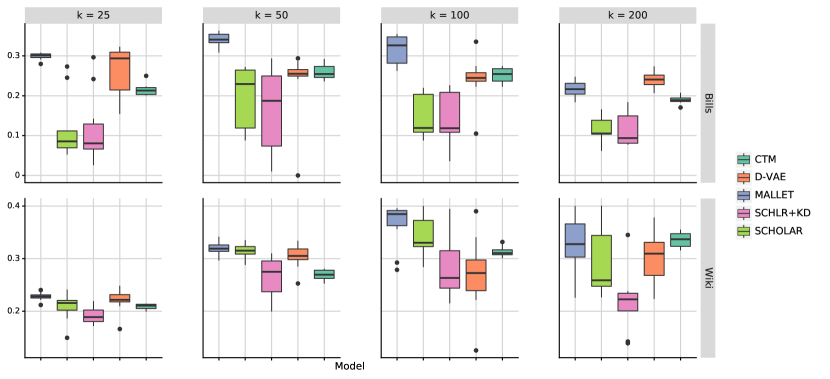

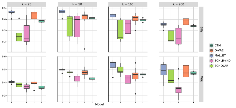
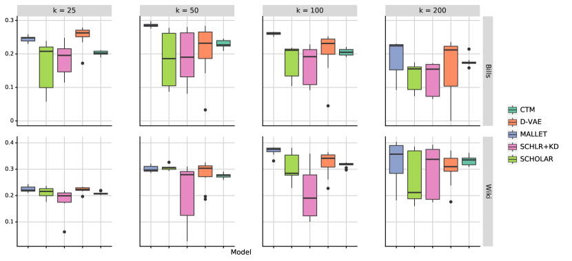
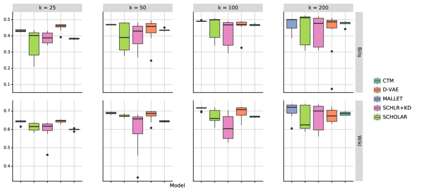
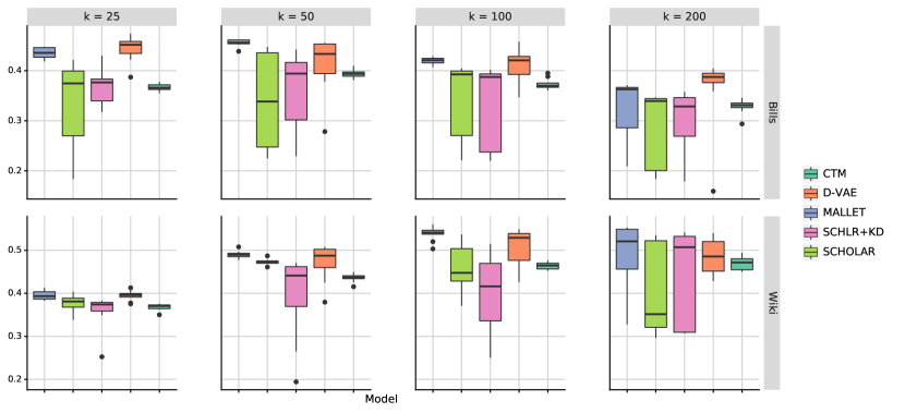
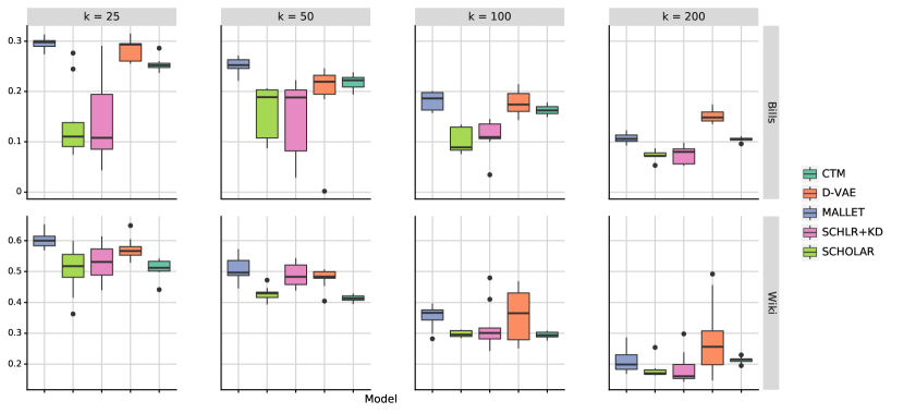
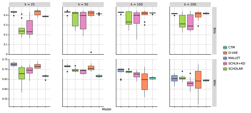
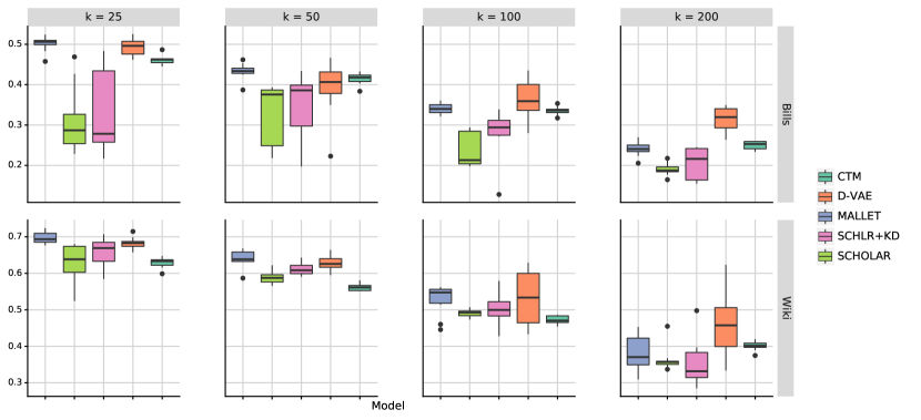
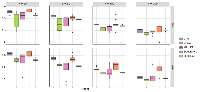
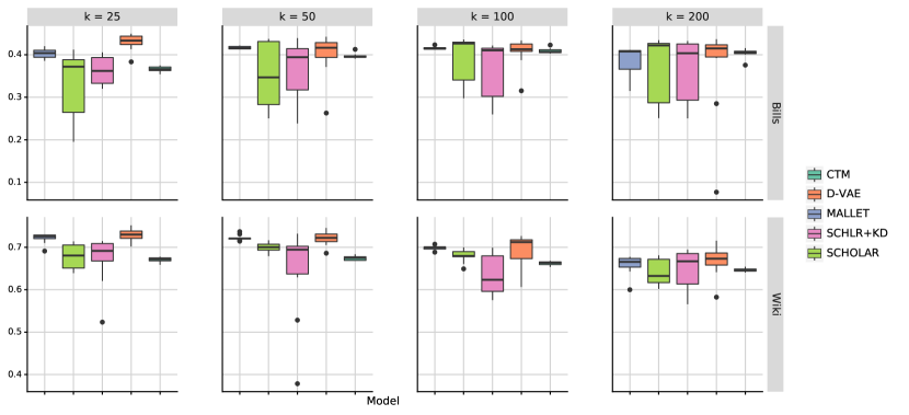
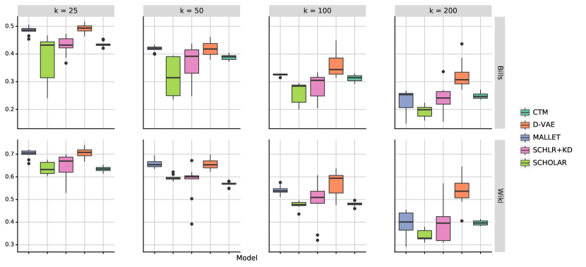
A.5 Additional ensembling results
In Table 8, we list the best-performing ensemble per model type, alongside a method that fares well across all models. For two out of the five models, the ensemble outperforms the median member in all 40 settings. Most ensembles improve upon the best member at least half the time. We also identify a set of hyperparameters (distance metric, , and clustering algorithm) that can ensemble the results of any of our models (Overall row in Table 8).
A.6 Compute infrastructure
We used AWS ParallelCluster to provide a cloud-computing computing cluster. Neural topic models ran on NVIDIA T4 GPUs using g4dn.xlarge instances with 16 GiB memory and 4 CPUs.151515https://aws.amazon.com/hpc/parallelcluster/ Mallet ran on CPU only, with m5d.2xlarge instances (with 32 GiB memory, 8 CPUs).161616See https://aws.amazon.com/ec2/instance-types/ for further details.