History of two mass loss processes in VY CMa

Abstract

Context. Red supergiant stars (RSGs, $M_{init}=10-40\mbox{$M_{\odot}$}$) are known to eject large amounts of material, as much as half of their initial mass during this evolutionary phase. However, the processes powering the mass ejection in low- and intermediate-mass stars do not work for RSGs and the mechanism that drives the ejection remains unknown. Different mechanisms have been proposed as responsible for this mass ejection including Alfvén waves, large convective cells, and magnetohydrodynamical (MHD) disturbances at the photosphere, but so far little is known about the actual processes taking place in these objects.

Aims. Here we present high angular resolution interferometric ALMA maps of VY CMa continuum and molecular emission, which resolve the structure of the ejecta with unprecedented detail. The study of the molecular emission from the ejecta around evolved stars has been shown to be an essential tool in determining the characteristics of the mass loss ejections. Our aim is thus to use the information provided by these observations to understand the ejections undergone by VY CMa and to determine their possible origins.

Methods. We inspected the kinematics of molecular emission observed. We obtained position-velocity diagrams and reconstructed the 3D structure of the gas traced by the different species. It allowed us to study the morphology and kinematics of the gas traced by the different species surrounding VY CMa.

Results. Two types of ejecta are clearly observed: extended, irregular, and vast ejecta surrounding the star that are carved by localized fast outflows. The structure of the outflows is found to be particularly flat. We present a 3D reconstruction of these outflows and proof of the carving. This indicates that two different mass loss processes take place in this massive star. We tentatively propose the physical cause for the formation of both types of structures. These results provide essential information on the mass loss processes of RSGs and thus of their further evolution.

1 Introduction

Asymptotic giant branch (AGB) stars and red supergiant (RSG) stars, two categories of evolved stars, are known to be among the main dust factories in the Universe. Along with this dust, these objects reinject gas composed by processed material into the interstellar medium (ISM), and are thus essential to the chemical enrichment of galaxies (Höfner & Olofsson, 2018). While the contribution of RSG stars to the ISM dust in the Milky Way is expected to be low ($\sim$1%), they are thought to be the dominant source of ISM dust in starburst galaxies and in galaxies presenting long loop-back times (i.e., very distant galaxies) (Massey et al., 2008). The mass loss of these objects determines their fate (Smith, 2014): which objects reach the supernova phase, when this phase takes place, and the contribution of heavy elements to the ISM by these stars.

The mechanism responsible for the mass ejection in low- and intermediate-mass evolved giant stars ($M_{init}\sim 0.6-9\mbox{$M_{\odot}$}$) during their evolution along the AGB is relatively well established (Höfner & Olofsson, 2018). Due to stellar pulsations a quasi-static layer is formed around the star. In this layer the temperature is low enough to activate dust formation. The radiation pressure on the dust and the dust–gas coupling (Goldreich & Scoville, 1976) generate an approximately isotropic mass ejection.

Red supergiant stars are also known to lose large amounts of mass (de Jager, 1998). However, the pulsations of these stars are irregular and, more importantly, they have low amplitude (Josselin & Plez, 2007), which prevents the formation of the quasi-static layer where the dust formation could take place. Therefore, the AGB dust-driven mass loss mechanism does not work in the case of massive stars. While several possibilities have been proposed, the actual mechanisms that drive mass loss ejection in this type of stars have not yet been established (Bennett, 2010).

Studying the mass ejections around evolved stars has been found to be a powerful tool to understand the mass loss processes. In particular, the molecular emission from these ejecta provides spatio-kinematical information which allows us to reconstruct the events generating the ejection. These results provide strong constraints on the mechanisms driving those events.

Large convective cells have been identified in the closest RSG star, Betelgeuse (Lim et al., 1998), and have been associated with a trefoil structure observed around the photosphere of the star with the ALMA interferometer (Kervella et al., 2018). However, despite Betelgeuse’s relatively close distance (197 pc; Harper et al., 2008), the structure of the inner ejecta has not been resolved enough to disentangle between the different mass ejection mechanisms proposed.

On the other hand, VY CMa, a RSG located at a distance of 1.2 kpc (Zhang et al., 2012), presents a massive ejecta very rich in molecular species with an oxygen-rich chemistry (Ziurys et al., 2007; Tenenbaum et al., 2010) that can be studied in detail. The ejecta around this object is known to present a complex structure (e.g., as seen in Hubble Space Telescope images Kastner & Weintraub, 1998; Humphreys et al., 2007). Accordingly, the molecular lines show complicated line profiles, which suggest a heterogeneous spatio-kinematical structure. Thanks to the use of the ALMA interferometer, in particular to the molecular maps obtained by De Beck et al. (2015), Decin et al. (2016), and O’Gorman et al. (2015), among others, the complexity observed in the outer regions is also observed in the innermost areas of the ejecta.

Richards et al. (2014) identified two main regions (see Fig. 1): $VY$, which corresponds to the central star and presents a N-E elongation, and $C$, which is associated with very cold and dense dust ($T_{d}\sim 100\,K$, $\sim 1.2\times 10^{-3}\mbox{$M_{\odot}$}$) (Vlemmings et al., 2017). The maps obtained by De Beck et al. (2015) for the TiO₂ emission and Decin et al. (2016) for the NaCl emission present the same spatial features, for a spatial resolution of $\sim$0.^′′1–0.^′′2. These regions have also been identified in our maps with higher spatial resolution (Fig. 1). Other regions identified in previous works are also shown in Fig. 1.

O’Gorman et al. (2015) estimated that the mass loss events responsible for the formation of the different regions surrounding VY took 30–50 years. These authors suggest that on these timescales the formation of these structures cannot be a consequence of the presence of convective cells; although the direction of the ejections took place at different angles, the duration of the mass ejections was relatively long compared to typical timescales of the convective cells ($\sim 150$ days). They suggested that the formation of long-lived cold spots at the stellar atmosphere, related with magnetic fields, where dust can be formed and drive a somewhat collimated mass ejection, is a better mechanism responsible for the formation of the structures observed. It is worth noting that these cold-spot induced ejections would present a velocity field similar to the ordinary dust-driven mass ejections, reaching a terminal velocity related with the dust properties and the luminosity of the star.

The origin of the structures observed toward VY CMa has also been associated with a dimming period undergone by VY CMa $\sim$ 100 years ago (Kamiński, 2019). A similar process seems to be taking place now in Betelgeuse. In that sense Betelgeuse might be an object at an earlier stage than VY CMa. Recent works (Levesque & Massey, 2020) suggest that the decrease in its brightness is related with the formation of dust in our direction. However, an intensity decrease has also been observed at millimeter-wavelengths which might suggest that the changes are not due to the formation of a localized mass ejection in our direction, but to changes in the photosphere itself (Dharmawardena et al., 2020). More recently it has been suggested that both effects might be responsible for the dimming observed in this object, a local decrease in the photospheric temperature that triggered the dust formation and ejection of material in our direction (Montargès et al., 2021).

In order to study the characteristics of the ejecta, and the processes driving these mass ejections we obtained ALMA molecular maps of VY CMa with an angular resolution of $\sim 25-35$ mas at the spectral range $\sim$216.20 – 235.45 GHz which covers molecular lines from species such as NaCl, H₂S, H₂O, SiO, SiS, ¹³CO, and PN, among others (Table 1). The obtained maps provide unprecedented detail of the structure of the ejecta that allow us to propose for the first time a 3D view of the ejecta. The description of the observations and data reduction is presented in Sect. 2 of the present work.

2 Observations

The observations of VY CMa were performed with the ALMA interferometer (project code 2017.1.00558.S, in Cycle 5) during a unique observing execution of 1.3h in October 2017. Forty minutes of acquisitions were obtained on the source, with 51 antennas. Baselines ranged from 41m to 16km, providing an angular resolution $\sim 0\mbox{\hbox to0.0pt{.\hss}${}^{\prime\prime}$}025$ and with maximum recoverable scale for the most extended emission of $0\mbox{\hbox to0.0pt{.\hss}${}^{\prime\prime}$}36$. The amount of precipitable water vapor was $\sim\,1$mm, humidity 10-35%, ambient temperatures $\sim-4^{\circ}$, and system temperatures 60–80 K. Four spectral windows of 1.875 GHz bandwidth were centered at the sky frequencies 217.090, 219.974, 232.641, and 234.516 GHz, with spectral resolutions of 1.35, 1.33, 1.26, and 1.25 km/s.

The bright point-like source J0522-3627 was observed to calibrate the bandpass, and was also set as absolute flux reference, with fluxes of 4.17, 4.16, 4.10, and 4.09 Jy for each spectral window. Observations of J0725-2640 were performed every two minutes to calibrate amplitude and phase gains in time. The phase rms after calibration was 32 deg.

The standard phase calibration was subsequently improved by self-calibration on the continuum emission from the source. Imaging restoration was made with a robust weighting. Image synthesis was made by using the cleaning method SDI(Steer et al., 1984). The obtained synthetic beam is 29 $\times$ 25 mas, and the brightness rms per channel is $\sim$ 0.15 mJy Beam^-1. The brightness rms achieved in the continuum map is in the range 0.028–0.052 mJy Beam^-1 depending on the spectral window (spw), with a continuum emission peak at R.A. 07^h22^m58.^s323 Dec. -25^∘46^′03.^′′00 (J2000).

Continuum was also subtracted by averaging the visibility channels free of molecular emission for each spectral window, and subtracting these continuum visibilities from the original data. Calibration was performed with the CASA software package, and data analysis with GILDAS and Astructures.

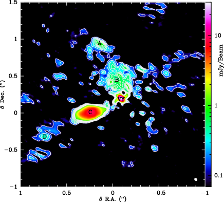
Figure 1: Continuum emission obtained from the ALMA data at $\lambda=\,1\,mm$. The half power beam-width is $0\mbox{\hbox to0.0pt{.\hss}${}^{\prime\prime}$}04\times 0\mbox{\hbox to0.0pt{.\hss}${}^{\prime\prime}$}03$ with a position angle of 29^∘ (see bottom right corner). The contours correspond to steps of 5$\sigma$ ($\sigma$ = 0.023 mJy/beam). The labels of the different regions follow Kamiński (2019).

3 Structure of the ejecta

The ALMA data covered a large variety of species (Table 1). The different species were identified using MADEX (Cernicharo, 2012). Some of these lines were detected, but are too weak to obtain a usable map. Our new ALMA maps reveal that the molecular and continuum emission can be divided into two general types. The continuum emission (Fig. 1) presents relatively compact structures already identified in previous works (Richards et al., 2014; O’Gorman et al., 2015; De Beck et al., 2015). These structures are also clearly traced by certain species such as H₂S or NaCl. On the other hand, the emission from SiO, SiS, SO or ¹³CO presents a more extended emission. See Fig. 2 for a general reference of these structures. The extended emission is partially filtered out. However, it can be clearly seen that these large-scale emission data present hollow regions.

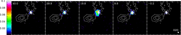
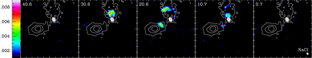
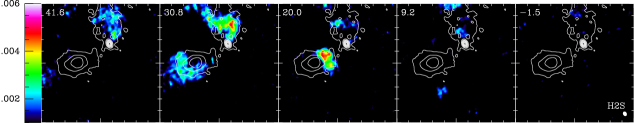
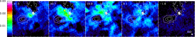
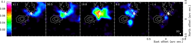
Figure 2: Channel maps of some lines showing the complexity of VY CMa ejecta (continuum shown in contours). From top to bottom in color: H₂O $v=2$ $5_{5,0}-6_{4,3}$; NaCl 18–17; H₂S 2_2,0–2_1,1 SiO 5–4; SO $5_{6}-4_{5}$. The value of $V_{LSR}$ of each panel is shown in the upper left corner. The HPBW is $0\mbox{\hbox to0.0pt{.\hss}${}^{\prime\prime}$}04\times 0\mbox{\hbox to0.0pt{.\hss}${}^{\prime\prime}$}03$ with a P.A. of 29^∘ (see the bottom right corner of the last panel). The continuum emission is shown in white contours.

The emission of SiO and other species such as SO or SO₂ is absent in those regions where H₂S emission arises (see Fig. 2 and Fig. 7 for a full SO channel map). In particular, SO presents a series of bubble-like structures in its ejecta. Thanks to the detailed radiative transfer modeling of the line emission of SO and SO₂ in this object, it has been noted that the origin of these species might be inner material swept up by high-velocity winds(Adande et al., 2013). While SiO is more ubiquitously distributed, SO would be a better tracer of the edge of these cavities.

As mentioned by O’Gorman et al. (2015), this extended ejecta seems to correspond to a quiescent, less localized mass ejection, that has been carved by recent collimated ejections. SiO and SO emission present clear signs of this carving, as the maps present no emission of these lines in the regions where the narrow outflows arise (see Fig 2).

In particular, we can identify in the first channels of Figs. 2 and 7 the SO emission surrounding the northern fast outflow, which is almost in the plane of the sky, but slightly tilted toward us. In the middle channels the SO emission surrounds clump $C$. Finally, the last channels show a shell that coincides with the rear outflow detected in the 3D reconstruction presented below. This clearly suggests that these localized jets have carved gas ejected previously. These holes formed in the quiescent ejecta by the collimated jets might be those inferred in previous works (Humphreys et al., 2019, 2021).

In addition, we find SiO and SO emission in the inner regions, closer to the central star. This indicates that the quiescent mass ejection has taken place both before and after the occurrence of the fast localized outflows.

Table 1: Parameters of the observed lines.

$\nu_{\mathrm{rest}}$ (MHz)	Molecule	Transition	$E_{\mathrm{up}}$ (K)
216531.44180	Na37Cl	16–17	93.6
216643.30424	SO2	222,20–221,21	248.5
216710.44359	p-H2S	22,0–21,1	84.0
216757.60348	SiS	12–11, v=1	1138.8
217104.91983	SiO	5–4	31.3
217817.65596	SiS	12–11	68.0
219376.92	U	–	–
219465.54552	SO2	222,20–221,21, v=2	993.7
219614.93595	NaCl	17-16 v=1	614.5
219776.66	U	–	–
219949.39633	SO	56–45	35.0
220165.25185	SO2	163,13–162,14, v=2	893.4
220330.80523	AlOH	7–6	42.3
220398.68354	13CO	2–1	15.9
231963.56981	TiO2	192,18–191,19	137.6
232628.58461	Si33S	13–12	78.2
232686.70000	o-H2O	55,0–64,3, v=2	3427.8
232031.09	U	–	–
232509.97689	NaCl	18–17 v=1	625.7
233116.41893	AlCl	17-16,	95.1
233664.46372	SiS	13–12 v=2	1150.1
234187.05727	SO2	283,25–282,26	403.1
234421.58220	SO2	166,10–175,13	213.3
234251.91247	NaCl	18–17	106.9
234812.96839	SiS	13–12 v=1	1150.1
234935.69126	PN	5–4	33.8
235130.60	U	–	–
235151.72126	SO2	42,2–31,3	19.0
235174.27	U	–	–

3.1 $VY-A$ & $VY-C$ ejecta

As mentioned above, we observed that the interferometric maps of NaCl $v=0,1$ and H₂S traced the collimated structures $A$ and $C$ observed in previous works (De Beck et al., 2015; Decin et al., 2016), which are also traced by the continuum (Fig. 1). We thus used the maps of these species to study the structure of the localized mass ejections. We obtained position–velocity (PV) diagrams of these line emissions along the main axis of the two structures connecting them with the central star $VY$. In the case of NaCl and H₂S these diagrams showed that these outflows present a straight-line shape; in other words, they follow a Hubble-like expansion velocity field ($V_{exp}\propto r$; see Fig. 3). In these PV maps we can see that while the ejecta C consists of a relatively simple outflow, the structure of the A outflow is more complex, probably as this latter structure is composed of different outflows. We note that the region $B$ is included in the $VY-A$ outflow, and we do not refer to it explicitly in the rest of the text. In order to fit the velocity field of these outflows, we took into account a twofold degeneracy. There is a series of pairs of values of the jet inclination with respect to the plane of the sky ($\theta$) and the value of the velocity constant ($V_{0}$), which would fit the velocity field of the outflow.

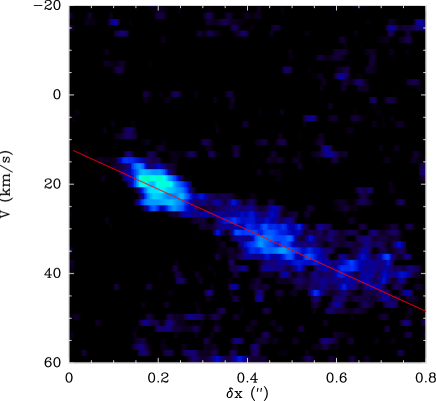
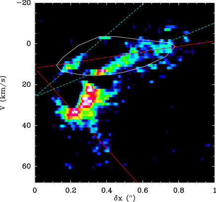
Figure 3: Position-velocity diagrams obtained for H₂S 2_2,0–2_1,1 along different directions. Left: PV obtained for H₂S 2_2,0–2_1,1 emission along the line connecting $VY$ and $C$. The red line corresponds to a linear jet with an inclination of 15^∘ with respect to the plane of the sky and $v=17\times r/0\mbox{\hbox to0.0pt{.\hss}${}^{\prime\prime}$}1\,\mbox{km\leavevmode\nobreak\ s${}^{-1}$}$ and $V_{\mathrm{LRS}}=12\mbox{km\leavevmode\nobreak\ s${}^{-1}$}$. Right: PV obtained for the same transition along the line connecting $VY$ and $A$. The red lines correspond to the same velocity field as in the left panel and an inclination with respect to the plane of the sky of 4.5^∘ for the upper jet and 30^∘ for the lower jet (see red lines). The white line surrounds the suggested structure of the northern jet (see text). The cyan line corresponds to $V_{\mathrm{LRS}}=26\mbox{km\leavevmode\nobreak\ s${}^{-1}$}$ (see text).

From the literature we know that the C outflow is close to the plane of the sky (Richards et al., 2014; De Beck et al., 2015; Kamiński, 2019). While the 3D model presented by Kamiński (2019) suggests that C is directly in the plane of the sky, spectral maps suggest that it is slightly tilted. We thus can assume that the inclination of C is equal to or lower than that of blob D, which was $\sim 15^{\circ}$ (Kamiński, 2019).

Assuming this inclination for the C jet, we found we could fit the expansion velocity to $v=17\times r/0\mbox{\hbox to0.0pt{.\hss}${}^{\prime\prime}$}1\,\mbox{km\leavevmode\nobreak\ s${}^{-1}$}$. Its important to note that this type of velocity field ($v\propto r$) cannot be created by the radiation pressure on dust grains, but a different mechanism might be the responsible for these ejections. This type of velocity field has been extensively observed in the post-AGB fast outflows. In addition, the fitting of the outflow connecting $VY$ and $C$ suggests the systemic velocity at $VY$ might not be 22 km s^-1 as previously thought (Decin et al., 2016; Richards et al., 2014), but $V_{LSR}=$12 km s^-1. This is compatible with the asymmetries observed by de De Beck et al. (2015) for the TiO₂ line profiles. Obtaining the value of $V_{LSR}$ as the mean velocity of the profile is useful for sources with an isotropic mass loss ejection, such as AGB stars, or for objects with symmetric mass ejections, such as some pre-planetary nebulae (pPNe). However, for cases like VY CMa, where the mass ejections seem to take place in different directions, this procedure might provide incorrect results.

The PV diagram obtained along the line connecting $VY$ and $A$ presents two main jets (Fig. 3-right), one jet pointing backward and a second larger jet closer to the plane of the sky and pointing toward the north. The $B$ region is composed of the emission of these two jets, while $A$ arises just from the latter. The jet pointing away from us suggests a source velocity similar to that of jet C, while the larger jet suggests a LSR velocity of 26 km s^-1. However, a careful inspection of the $VY$–$A$ ejecta suggests that we might not be detecting certain parts of this ejection, and that the different emitting regions that are within the area delimited by the white line in Fig.3, $right$, correspond to the same unique ejection. This is better seen in the 3D reconstruction (see Fig. 4). Nevertheless, the possibility of the $VY$–$A$ jet arising from $VY$ at 26 km s^-1 cannot be completely ruled out, and future observations will shed light on this fact.

If we impose the same velocity field, the inclination for the northern jet is 4.5^∘ and that of the rear jet is -30^∘. It is important to note that these jets accurately correspond to the hollows observed in the SO emission.

The value of $V_{\mathrm{LSR}}$ obtained corresponds to a position in the 3D structure of the ejecta. Tracing back the trajectory of the different outflows can be used to confirm the real position of the central star (see Fig. 4).

The extent of the $VY$–$C$ and $VY$–$A$ outflows is similar, around $\sim 0\mbox{\hbox to0.0pt{.\hss}${}^{\prime\prime}$}7-0\mbox{\hbox to0.0pt{.\hss}${}^{\prime\prime}$}8$, which corresponds to $1.3-1.5\times 10^{16}$cm, and reaches a velocity of $\sim 120-140\mbox{km\leavevmode\nobreak\ s${}^{-1}$}$ at the tip of these outflows. The formation of these structures took $\sim 50-60$ years, confirming the timescales suggested above (O’Gorman et al., 2015). It is worth noting that these high velocities are not observed in the line profiles due to the projection effects, which means that the ejection that dominates the width of the line profiles is that corresponding to the less localized and slower mass ejection.

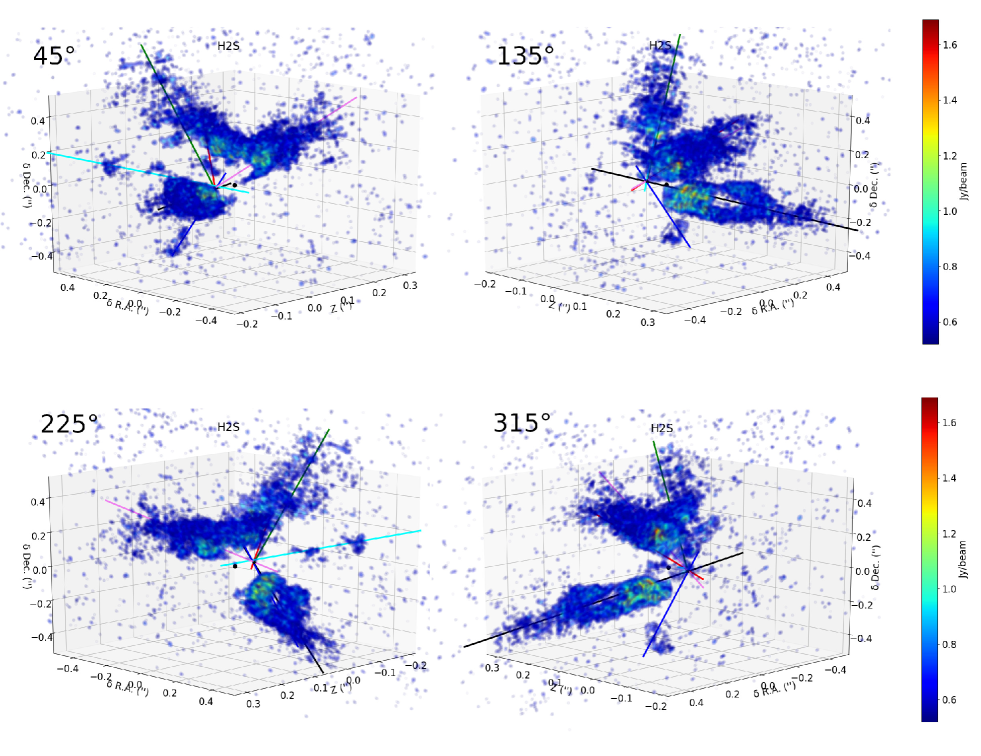
Figure 4: Reconstruction of the H₂S $2_{2,0}-2_{1,1}$ emission structure. The structure is generated for a flux with a S/N $\geq$3. The colored arrows correspond to the main axis of the different outflows, as shown in the videos. For more detail, see the video presenting the rotation of the H₂S structure. The angle is taken in the clockwise direction with respect to the line of sight.

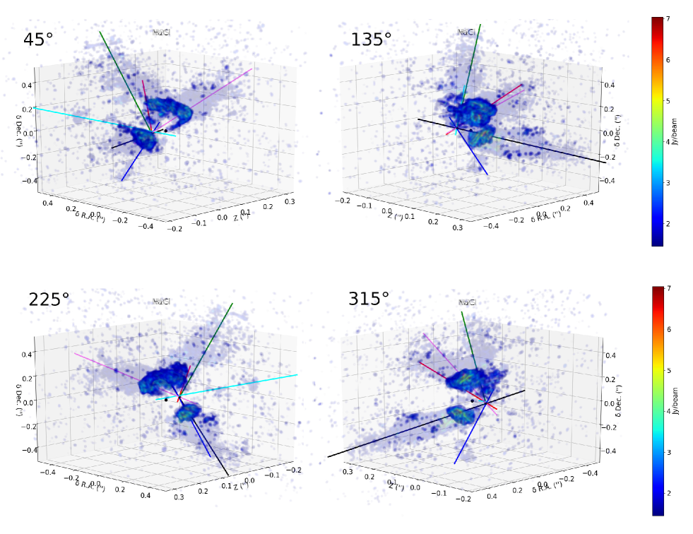
Figure 5: Reconstruction of the NaCl $J$=18–17 emission structure (colors) overplotted on the H₂S emission presented in Fig. 4 (transparent colors). The structure is generated for the flux with a S/N$\geq$3.

Figure 6: Profile of the ortho-H₂O $5_{5,0}-6_{4,3},v=2$ maser emission structure toward the maximum of the emission.

3.2 Three-dimensional reconstruction

Due to the complex structure of the ejecta we generated 3D structures imposing the expansion velocity field obtained from the PV diagrams using the Astructures code. Briefly, Astructures reads the data from a spectral cube, estimates the Gaussian noise from the cube, and crops out the data below a given threshold (i.e., 3$\sigma)$. The spectral maps consist of two spatial coordinates (R.A. and Dec.) and a velocity coordinate. The code plots the points in a flux scale following these coordinates. Assuming a given velocity field, this dimension can be transformed into a space dimension, allowing us to reconstruct a 3D spatial structure. In addition, to help us identify the different structures, the code rotates the structure around a selected axis, creating images for each rotation angle and a video.

The reconstructed structure is rotated to allow the inspection of the different elements. These 3D structures rotated are presented in Figs. 4 and 5 and in the videos associated with this work.

Thanks to the 3D reconstruction, at least six outflows can be identified in the structure obtained, especially from the H₂S maps (see red arrows in Fig. 4). Two outflows correspond to the structures observed in the continuum and molecular emission (De Beck et al., 2015; Decin et al., 2016; O’Gorman et al., 2015) (outflows $VY$–$C$ and $VY$–$A$), while we identified two other outflows placed behind the $VY$–$A$ outflow. For the last two outflows only bullet-like structures are visible. We cannot determine if the bullet-like structure of these outflows is real or due to a lack of S/N in the obtained maps.

On the contrary, the PV diagrams obtained from species like SiO or SO present very complex structures, probably as a consequence of swept-up and shocked regions (Adande et al., 2013). The flux filtering affects structures with scales larger than $\sim$0.^′′4. However, this only affects homogeneous structures. Inhomogeneous structures are preserved. Furthermore, under certain circumstances filtering the homogeneous large-scale structures allows a better tracing of the mid-size and small structures, due to the relative dynamic range.

The fast outflows observed are compatible with the bubble-like structures observed in SO (Fig. 7). In particular, in this figure we can see these shells as a consequence of the carving by the jets presented above, at $\sim 1.2\mbox{km\leavevmode\nobreak\ s${}^{-1}$}$, $\sim 30.5\mbox{km\leavevmode\nobreak\ s${}^{-1}$}$, and $\sim 59.7\mbox{km\leavevmode\nobreak\ s${}^{-1}$}$, and as a shell extending along the channels in the range $\sim 30-80\mbox{km\leavevmode\nobreak\ s${}^{-1}$}$. As mentioned, the velocity field of SO is particularly complex, and different from that observed for the fast outflows. This prevented a 3D reconstruction and a direct comparison of the structures traced by SO and H₂S. In order to inspect the relation of the fast outflows with the bubbles observed in SO, we plotted the H₂S emission (overplotted the SO channel maps), for which we modified the velocities of H₂S so the shells and the outflows coincide (see Fig. 7, where the velocity of both emissions are shown). This comparison shows that the outflows traced by H₂S and the shells probed by SO are related. In particular it suggests that the outflows are carving previous ejecta and forming cavities. This coincidence of the jets and the holes clearly suggests the existence of two mass loss processes, and the carving of previously ejected material by the fast outflows.

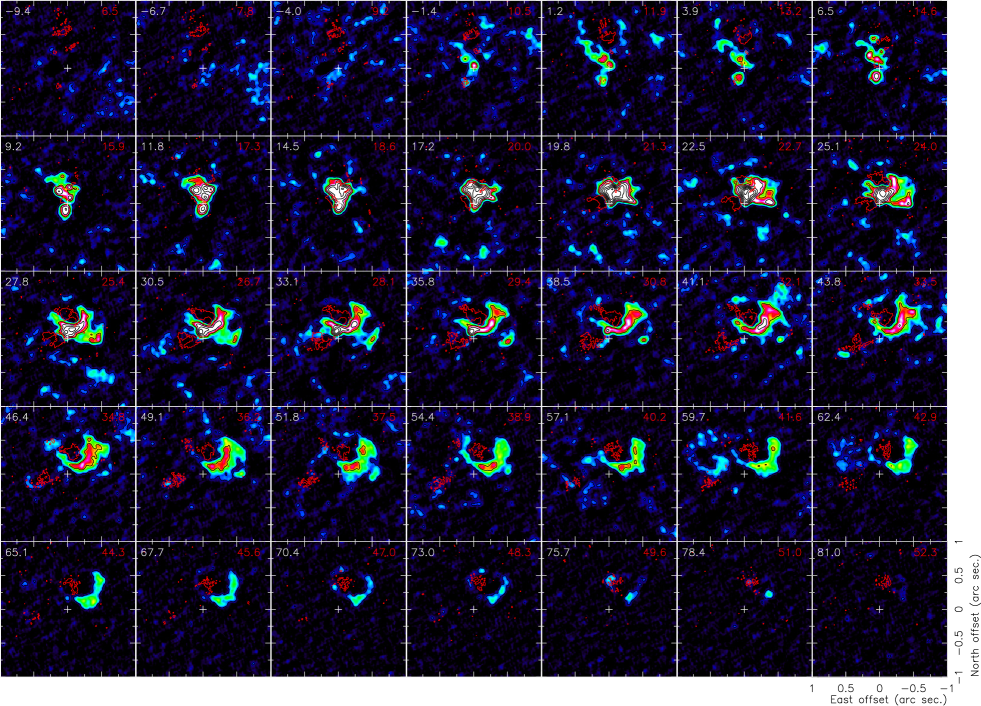
Figure 7: Comparison of the SO $5_{6}-4_{5}$ emission (colors and black contours) and H₂S 2_2,0–2_1,1(red contours). $V_{\mathrm{LSR}}$ for SO is shown in the upper left corner, while that of H₂S if shown in red in the upper right corner. A video is available as supplementary material.

3.3 Inner ejecta

We also obtained inteferometric maps of the maser emission of ortho-H₂O $5_{5,0}-6_{4,3}$, ${v_{2}=1}$ at 232 GHz. This emission presents a local intense peak at $\sim 12\mbox{km\leavevmode\nobreak\ s${}^{-1}$}$, which is located at R.A. 07^h22^m58.^s327 Dec. -25^∘46^′03.^′′06 (J2000). This maser was predicted to be located much closer to the star than the other water masers (Menten & Melnick, 1989). Since the pumping mechanism of the maser is the IR emission from the central star, and the velocity of the peak corresponds to what we found to be compatible with the origin of the fast outflows, we propose that the position of this peak might correspond with the real position of the central star. Furthermore, the peak position of the continuum is not compatible with the expected origin of the H₂S outflows. In a similar way to $V_{LSR}$, the general assumption that the peak of the continuum emission corresponds to the stellar position is valid in those cases where the ejection of dust is isotropic or presents some type of symmetry. The intense emission of molecular lines arising at the stellar photosphere, like that of the o-H₂O maser, could provide a more accurate determination of the position of the central star in those cases where the ejection of material is more chaotic.

At least two inner outflows have been identified from the o-H₂O $5_{5,0}-6_{4,3}$ $v_{2}=1$ emission. This emission is constrained to the innermost regions of the envelope around the star and is barely resolved (half power beam width, HPBW, $\sim 30\times 20$mas). The kinematic structure of this emission is particularly complex. In order to obtain a first approach to the structure, we assumed a velocity field similar to that for the outer outflows. These outflows can be seen in Fig. 8. The resolution is not high enough to resolve the structure of the outflows.

3.4 Position and systemic velocity of the star

In order to identify, and confirm, the position-$V_{\mathrm{LSR}}$ of the central star we identified and traced the main axis of the different fast outflows. In the 3D videos labeled “lines” we plotted the axis and the two positions for the central source as a filled star corresponding to a $V_{\mathrm{LSR}}=12\mbox{km\leavevmode\nobreak\ s${}^{-1}$}$ and a filled circle for $V_{\mathrm{LSR}}=22\mbox{km\leavevmode\nobreak\ s${}^{-1}$}$. It can be seen that the former value seems more compatible with the ejections. This can be seen also in Figs. 4 and 5. The R.A. and Dec. for the central source are those obtained from the water maser, but it worth noting that assuming the R.A. and Dec. position derived from the continuum provides a similar result (i.e., $V_{\mathrm{LSR}}=12\mbox{km\leavevmode\nobreak\ s${}^{-1}$}$).

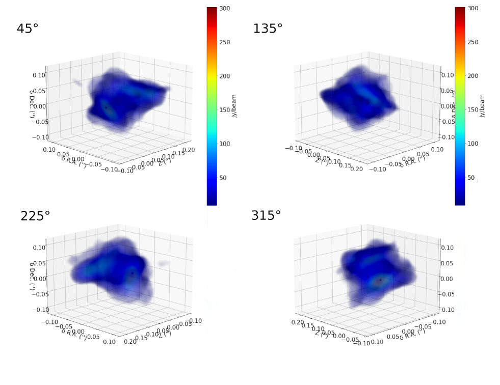
Figure 8: Reconstruction of the ortho-H₂O $5_{5,0}-6_{4,3},v_{2}=1$ maser emission structure. For more detail, see the video presenting the rotation of the o-H₂O structure. The structure is created for the flux above $3\sigma$.

4 Origin of the ejecta

4.1 Regular ejecta

By regular ejecta we mean that corresponding to the larger part of circumstellar material (the standard mass ejection of the source) and the ejecta that has been ejected during most of the time and that is traced by species like SiO or SO.

SiO and SO emission appears both in the outer regions and in the innermost areas where H₂S is not present, suggesting that most of the time the mass ejection takes place in a steady way, as traced by these species, and that under certain conditions massive fast narrow ejections take place.

This ejecta suggest mass loss ejections at different positions angles but not clearly localized. A good candidate for these events would be the convective cells observed toward Betelgeuse (Lim et al., 1998) or the recently proposed turbulence pressure (Kee et al., 2021), which would form an extended atmosphere where dust can be formed. These ejections would create ubiquitous (but not isotropic) ejecta around the star. In addition, these ejecta present a chemical footprint similar to that of high-mass O-rich AGB stars, in particular rich in SO and SO₂ lines. These spectral maps present cavities and hollow structures that can be related to fast outflows, such as those traced by H₂S carving these ejecta.

As already mentioned, the velocity field of these ejecta is very complex, probably due to the presence of swept-up material and the inhomogeneities of the mass loss ejection. However, the velocity field and the terminal velocity of the ejection are compatible with a mass ejection powered by radiation pressure on grains (i.e., $V_{\infty}=30-40\mbox{km\leavevmode\nobreak\ s${}^{-1}$}$ for these type of objects). It has been found that other massive evolved stars present similar wide profiles that are related to the high luminosity of these objects (Quintana-Lacaci, 2008). As mentioned above, the high-velocity wings arising from the outflows are not observed in the line profiles, due to projection effects, and it is the slowly expanding gas that is responsible for the line profile width observed.

4.2 Sporadic outflows

As shown above, more than six new outflows have been detected with enough spatial and spectral resolution to reconstruct the structure of the ejecta and to derive their global characteristics. It has already been proposed that the mechanism driving these mass ejections might have a magnetic origin (O’Gorman et al., 2015; Vlemmings et al., 2017). Furthermore, the Hubble-like velocity field obtained suggests that the mechanism powering this ejection is not related to radiation pressure on dust grains formed on cold spots, but instead to energetic events similar to those responsible of the high-velocity outflows typical of post-AGB stars (Bujarrabal et al., 2001).

These jets are traced by H₂S and NaCl. The emission from these species has been associated with shocks and high-density regions, respectively (Arce et al., 2007; Quintana-Lacaci et al., 2016). Furthermore, H₂S has been claimed to be released from the ice mantles of cold dust (Goicoechea & Cuadrado, 2021), where H₂S is formed and later on released into the gas due to shocks.

The extended outflows are well resolved and are found to have a flattened geometry (Fig. 9) in one of the directions orthogonal to the axis of the ejection when compared with pPNe bipolar outflows (see, e.g., M1–92, Alcolea et al., 2007). The ratio of width to height is $\sim\,6$. A similar shape can be identified in the rest of the outflows observed (except for those of H₂O which are not well resolved). This flatness is not an effect of the velocity field assumed, and derived by the PV diagrams. It is reproduced for different outflows which expand along different directions. In addition, we have modified the velocity law from constant expansion to higher exponential orders, and this flatness is maintained. Therefore, we claim that the flatness seems to be an inherent characteristic of the fast outflows observed, and thus it has to be explored in order to understand the mass ejection of this object.

The SO structure that seems to surround the rear H₂S jet presents a shrinking tubular structure. This tubular structure also seems flatter in the vertical axis compared with the horizontal one (see Fig. 7). We inspected how certain mechanisms could be responsible for the formation of such flat structures.

4.2.1 CME-like ejections. Linear momentum estimate.

The presence of cold starspots alone could not generate the structures observed as they usually show a roughly circular shape, and the produced outflows are expected to have a similar similar cross section orthogonal to their outflow axes. However, in the magnetically active regions of the stellar surface two mechanisms can generate outflows with the same shape as those observed in our ALMA maps. These mechanisms are the sunspot groupings and the coronal mass ejections (CMEs), which create elongated features in the stellar surface. The formation of a helmet streamer, a close magnetic loop that generates bright loop-like structures, and the subsequent CME in general takes place in active regions of the stellar surface where cold-spot grouping also takes place. On the other hand, a cold-spot grouping is unlikely to generate the shape of the ejections presented here, which in fact resembles the structure of the helmet streamers (Glukhov, 1997) and the final stages of the CMEs (Gibson & Low, 1998). Moreover, the theoretical reconstruction of an observed fast solar CME (Jin et al., 2013) shows a structure more elongated in one of the dimensions than in the other. In particular, this CME presents a structure similar to that observed in NaCl emission (Fig. 5). It has been suggested that CME events might be an important source of mass loss in active stars (Argiroffi et al., 2019).

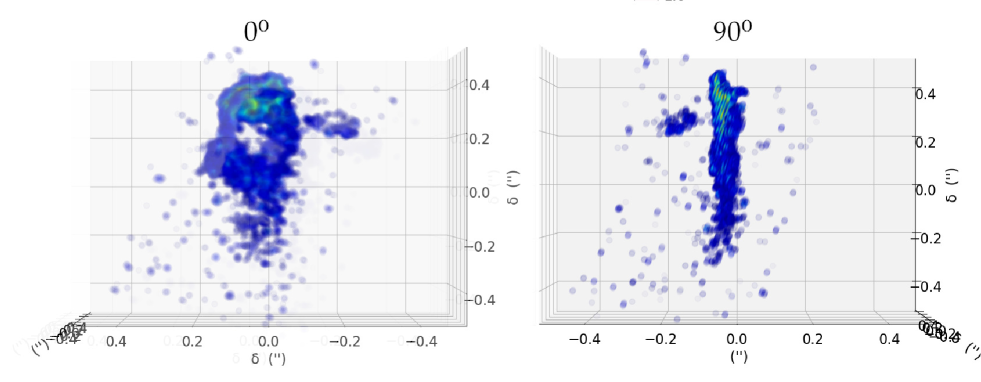
Figure 9: Reconstruction of the H₂S emission presented face-on and tilted 90^∘.

Coronal mass ejections are expected to present cold plasma escaping from the stellar atmosphere (Argiroffi et al., 2019) and the presence of X-rays. However, X-rays have not been detected toward VY CMa (Montez et al., 2015). This non-detection might be due to the disappearance of the CME eruption. As future collimated ejections or dimming events take place, target-of-opportunity X-ray observations might be useful to confirm the processes powering the ejections.

It is important to check, beyond the pure morphological similarity cited above, whether a CME can drive enough momentum to form a structure like those observed in VY CMa. We focus on the C outflow since it is the most massive ejection (O’Gorman et al., 2015), and especially because its properties can be accurately determined as it is isolated compared with the rest of the fast outflows.

We adopt the higher value for the dust mass of C derived by O’Gorman et al. (2015) with a gas-to-dust ratio of 200. The total mass of the outflow is therefore 0.05$M_{\odot}$. Other authors (Kamiński, 2019) have derived higher values for clump C; however, these values are extremely uncertain. The total momentum driven by this ejection assuming the Hubble velocity field deduced above and a constant mass distribution along the ejecta is $P=9.30\times 10^{38}$ g cm s^-1.

To estimate the momentum driven by a CME, we followed the discussion presented by Welsch (2018). In this work the author estimates a momentum transfer of 1 (g cm s^-1) per cm² per second for a magnetic field of 3 G, being this momentum transfer rate proportional to the perpendicular magnetic field $B_{\perp}$.

The size of the cold spots in the RSGs has been found (Künstler et al., 2015) to reach sizes of $2.8\times 10^{23}$ cm², and the time estimated for the formation of the C-outflow is $\sim$50 years. The magnetic field needed to provide the amount of momentum derived above is $\sim$5kG.

The magnetic field of VY CMa has been estimated to reach a strength of 1 kG at the surface of the star (Vlemmings et al., 2002), and more recently up to 50 kG (Shinnaga et al., 2017) assuming a toroidal magnetic configuration. These latter authors suggest that such strong magnetic fields are unlikely to occur since these objects are expected to have a slow rotation (Monnier et al., 1999), a large radius, and low temperatures, and thus they suggest that the strength of the field should be somewhat lower and more locally enhanced. However, higher rotation velocities have been observed in other RSGs (Wheeler et al., 2017) and planet engulfment has been proposed as a source of increasing this velocity, causing an enhancement of the dynamo and of the magnetic field (Privitera et al., 2016). In addition, previous studies (Vlemmings et al., 2017) also suggested that magnetic field distribution seems to confirm that C mass ejection is linked to the magnetic field.

In summary, the structure, the magnetic field strength, and the position angle (P.A.) of the different jets, and also the Hubble-like velocity field therefore seem compatible with outflows of magnetic origin, for example coronal mass ejections. A cold spot could also be responsible for the magnetically driven ejections, but not as a consequence of radiation pressure on newly formed dust, as mentioned above.

The formation of the fast outflows is estimated to have taken several tens of years, and thus stellar rotation might leave an imprint on the shape of the ejecta. The rotation velocity of RSGs is estimated to be $\sim$1km s^-1 (typical for RSG stars, Zhang et al., 2012), while for some objects such as Betelgeuse values as high as 15km s^-1 have been derived (Wheeler et al., 2017). With a stellar radius of VY CMa of $R_{\star}=9.9\times 10^{13}$cm (Wittkowski et al., 2012) the effect of the rotation should be seen in a collimated outflow with the formation times derived. This scenario is explored in 4.2.2.

4.2.2 Sprinkler model

If we assume that the flatness of the fast outflows is itself a consequence of a fast and collimated ejection combined with the stellar rotation, we should be able to find an angle that would be compatible with all these ejections (i.e., the rotation axis). In this case, all the flat structures would be constrained within a single latitude angle ($\theta_{i}$) with respect to the rotation axis for each fast ejection.

In this sense, we have found a particular angle ($\sim$95^∘) around the R.A. axis, which seems to be compatible with this scenario. This means that the rotation axis of VY  CMa would be approximately pole-on. This rotated structure is presented in Fig. 10, with the rotation axis as $Z$.

In addition, we created a simple model to simulate the creation of these structures. The model consists of a position at the photosphere of the star from which a certain gas ejection takes place. We adopted the velocity law from the PV diagram, a rotation velocity of 1 km s^-1 (typical for RSG stars; Zhang et al., 2012), and adapted the lapse of activity of the ejection ($t_{e}$) with an expansion velocity moduled by a sinusoidal so it is at a minimum when the ejection starts and finishes (at $t_{e}$) and reaches a maximum at $t_{e}/2$. In any case, it is important to bear in mind that, as mentioned above, higher rotation velocities have been inferred for other objects, for example $\sim$15km s^-1 for Betelgeuse (Wheeler et al., 2017).

The parameters of each ejection are presented in Table 2. We initiate a rotation of the star with a given $v_{rot}$ at $\phi_{0}=0$. The parameters $\theta_{i}$ and $\phi_{i}$ indicate the position and moment when the ejection starts, and $t_{e}$ the duration of the ejection; $\theta_{i}$ is the latitude of the ejecting spot and $\phi_{i}$ the rotation angle. We first modeled the ejection corresponding to clump $C$ and used it as a starting point to fit the rest of the fast outflows. In particular we found that we had to reduce the velocity by 10% for outflows 3–5, although the ejection time could be maintained. The result of our fitting of the sprinkler ejections to the observed H₂S structures is presented in Fig. 10. The different extents of the ejections in Fig. 10 are due to the fact that the ejections took place at different times.

Table 2: Parameters of the Sprinkler model outflows. The rotation velocity of the star is 1km s^-1. $V_{16}$ is the value for a Hubble-like expansion velocity at 10¹⁶cm.

Outflow	$\theta_{i}$ (∘)	$\phi_{i}$ (∘)	$V_{16}$ (km s-1)	$t_{e}$ (yr)
1	100	190	94.4	10
2	85	287	94.4	10
3	140	320	85.9	10
4	100	260	85.9	10
5	120	300	85.9	10

This is a simple approximation that confirms that the molecular emission observed for the fast outflows can be formed in this manner. The ejection time depends directly on the rotation velocity. In general, we find that $t_{e}=120/V_{rot}$[months s km^-1]. Therefore, for a $V_{rot}=15\mbox{km\leavevmode\nobreak\ s${}^{-1}$}$ the value of $t_{e}$ would be eight months. It is worth noting that the high magnetic field observed could be a consequence of an enhanced dynamo and due to high rotation velocities. In these cases we would expect low $t_{e}$.

We could also estimate the lapse between the different ejections. For a rotation velocity of 1km s^-1 we found that the time between the ejections was in the range $\sim$1 – 6 years, being the time between the first and the last ejection $\sim$11 years. For a $v_{rot}$ of 15km s^-1 the range would be $\sim$1 – 5 months and $\sim$9 months between the first and last ejection.

It is also important to note that $t_{e}$ just takes into account the time when a particular spot at the star is ejecting material. Once this ejection stops, the structure evolves given an expansion velocity until the observed structures are created.

It is worth noting that the arcs observed at larger scales Humphreys et al. (2007) resemble the fast outflows traced by H₂S and may have been produced by the same mechanism in the past.

5 Discussion

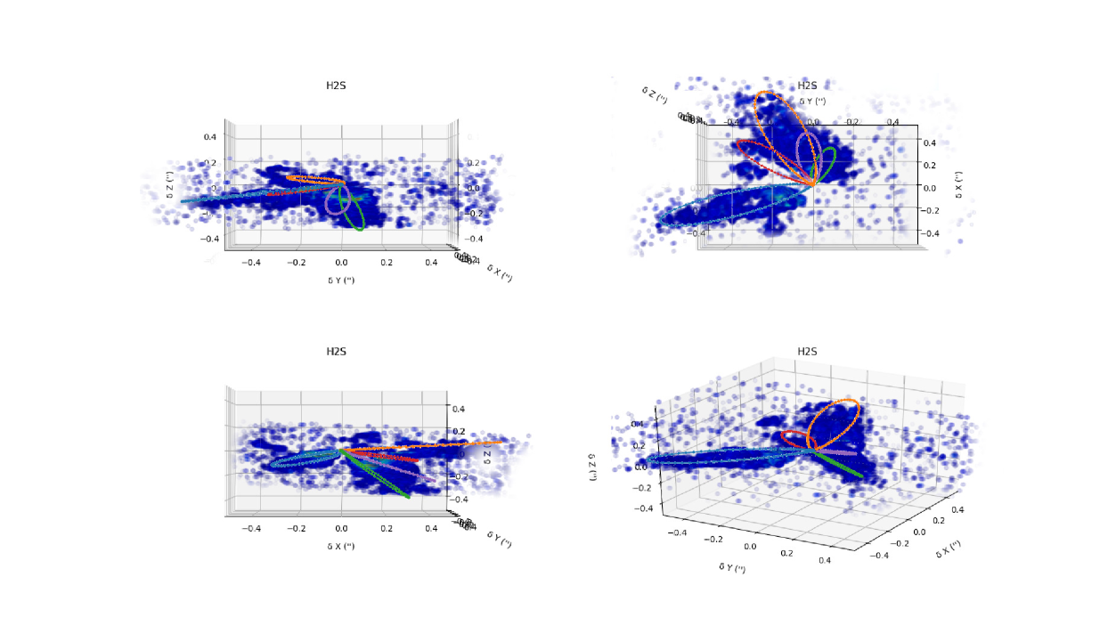
Figure 10: H₂S emission rotated so that the rotation axis corresponds to the Z-axis, overplotted to the result of the sprinkler model applied to five ejections.

The data we presented seem to support the claim (O’Gorman et al., 2015) that the mass ejection in this object occurs in two different ways: a somewhat ubiquitous and steady mass ejection, with chemical properties of O-rich objects (SiO, SO, SO₂) and fast collimated outflows taking place at random directions in which the sulfur is mainly constrained into H₂S. The SO and SO₂ emission would trace swept-up material with high density. The former ejections are likely due to convective cells, which would generate an irregular and extended atmosphere of circumstellar gas where most of the sulfur would be in the form of SO and SO₂, while another process, probably of magnetic origin, would generate fast outflows of gas and dust, which, when colliding with the surrounding material, would form H₂S by shocks or evaporate H₂S from dust (Arce et al., 2007).

Interestingly, Danilovich et al. (2017) found that only O-rich stars with higher mass loss rates present significant amounts of H₂S in their ejecta. This, together with the above-mentioned relation between H₂S and jets, seems to suggest that most massive stars will eventually present shocks that alter their chemistry from the standard O-rich where most sulfur is in form of SO and SO₂ to a relevant presence of H₂S.

We propose that at a certain moment of its RSG evolution the surface of VY CMa became magnetically active and generated intense magnetically driven mass ejections. Certain processes have been proposed as being responsible for generating this type of activity in massive evolved stars, such as the appearance of a local dynamo in the giant convective cells (Aurière et al., 2010) or an enhancement in the stellar dynamo by the engulfment of planets (Privitera et al., 2016). These ejections would have generated anisotropical fast outflows like those presented in this work.

Recent studies of other RSG stars reveal similar characteristics to VY CMa. In the particular case of $\mu$ Cep, CO observations also suggest two different mechanisms responsible for the ejecta around this object (Montargès et al., 2019), one responsible for the formation of a slow outflow and the other for the localized mass ejections. The authors of that work adopted a constant velocity field for both types of outflows, but they also suggest that this might not apply to $\mu$ Cep clump C2. This might also be the case of Betelgeuse (Levesque & Massey, 2020).

6 Conclusions

In summary, thanks to the spatial and spectral resolution of ALMA we were able to detect previously unidentified spatial features of and found global characteristics of the outflows taking place in VY CMa. In particular the observations confirm that the structures observed are produced by two types of mass ejections:

• A slow wind, which might be powered by mechanisms such as the large convective cells on the surface (Lim et al., 1998) that would form an extended warm atmosphere where dust formation and the subsequent radiation pressure on dust grains produce a smooth mass ejection. This ejection would not be either isotropic or strongly localized, but would generate an inhomogenous ejecta surrounding the object. The expansion velocity of this shell would be in the typical range for massive evolved stars (30–40km s^-1).

• A collimated wind, with a Hubble expansion law and reaching velocities up to 100km s^-1 similar to those observed in the post-AGB phase, which would carve the previous ejecta. These fast winds could not be due to radiation pressure on dust formed at long-lived cold spots, as indicated by the velocity field, but were caused by other mechanisms. Coronal mass ejections or other magnetically driven mass ejection might be responsible for these ejections. These mass ejections could be related to local enhancements of the magnetic field (Shinnaga et al., 2017).

In the general context of massive star evolution, and in particular of the mass loss processes determining the path of these objects during their last throes, the results presented here have a key relevance. The data presented show, for the first time, that mass loss within this phase can take place in two completely different ways. A future systematic study of RSGs and the characteristics of their ejecta, as well as detailed jet modeling to fit the structures will allow us to determine the characteristics favoring each type of mass event and the mechanism powering them. Two of the questions that should be addressed given the new mass loss paradigm suggested in this work are whether the slow expanding wind is the standard way these objects eject material, and if the jets are restricted only to those RSGs presenting higher rotation velocities and strong dynamos.