Prospects for Constraining the Yukawa Gravity with Pulsars around Sagittarius A*

Abstract

The discovery of radio pulsars (PSRs) around the supermassive black hole (SMBH) in our Galactic Center (GC), Sagittarius A* (Sgr A*), will have significant implications for tests of gravity. In this paper, we predict restrictions on the parameters of the Yukawa gravity by timing a pulsar around Sgr A* with a variety of orbital parameters. Based on a realistic timing accuracy of the times of arrival (TOAs), $\sigma_{\rm TOA}=100\,\mu{\rm s}$, and using a number of 960 TOAs in a 20-yr observation, our numerical simulations show that the PSR-SMBH system will improve current tests of the Yukawa gravity when the range of the Yukawa interaction varies between $10^{1}$–$10^{4}\,{\rm AU}$, and it can limit the graviton mass to be $m_{g}\lesssim 10^{-24}\,{\rm eV}/c^{2}$.

1 Introduction

General relativity (GR) has stood up to a variety of tests since its proposal by Albert Einstein in 1915 [1, 2]. However, the phenomena of dark matter [3] and dark energy [4] have posed a great challenge to GR and inspired proposals for a series of modified gravity theories [5, 6]. Theories of massive gravity [7], which add a mass term to the graviton, have aroused wide interest. Some earlier theoretical difficulties were eventually overcome, for example, in the resolution to the van Dam-Veltman-Zakharov (vDVZ) discontinuity [8, 9] via the Vainshtein mechanism [10]. There are many massive gravity theories [11], and a popular parametrization is called the Yukawa potential theory. In this theory, the gravitational potential is Yukawa-type suppressed [7, 12, 13, 14]. For a point mass source, the gravitational potential is expressed as,

$$\phi(r)=-\frac{GM}{(1+\alpha)r}\left(1+\alpha{\rm e}^{-\frac{r}{\Lambda}}\right),$$ (1.1)

where $G$ is the gravitational constant, $M$ is the mass of the central object, $r$ is the distance to central object, $\alpha$ and $\Lambda$ represent the strength and the range of the Yukawa interaction respectively. According to Eq. (1.1), when the length scale $r$ of a system is much less than the range of the Yukawa interaction $\Lambda$, the Newtonian potential $\phi_{\rm N}(r)\propto-GM/r$ is recovered so, augmented with post-Newtonian (PN) corrections, it passes the stringent gravity tests from the Solar system when $\Lambda\gg 1$ AU [15, 16]. When $r$ is comparable to $\Lambda$, the Yukawa gravity will show clear deviations from the Newtonian inverse-square law. If $r\gg\Lambda$, a Newtonian-like potential is recovered but with a different gravitational constant, $G_{*}=G/(1+\alpha)$. The change of gravitational constant has been successfully used to account for the observational rotation curves of spiral galaxies in a special case of $\alpha=1/3$ [17].

There are generally two ways to constrain the parameters of the Yukawa gravity. The first way is to obtain the constraints on the strength of the Yukawa interaction $\alpha$ as a function of the range of the Yukawa interaction $\Lambda$, which is used to search for new kinds of interactions, the so-called fifth force [15, 18]. Thus the Yukawa gravity can be a probe to seek for new kinds of interactions and fundamental fields, which could be candidates for dark matter and dark energy [19, 20, 16]. Due to the characteristics of the Yukawa potential (1.1), the optimal limit on $\alpha$ at a certain $\Lambda$ is usually obtained when the system scale $r$ is similar to $\Lambda$. Therefore, to fully explore the Yukawa gravity, it is necessary to carry out tests at a wide range of length scales. Tests have been conducted at various length scales, such as torsion oscillators at the laboratory scale [21, 22, 23], LAser GEOdynamic Satellite (LAGEOS) at a length scale of the Earth [24], and Lunar Laser Ranging (LLR) [25, 26] at the Earth-Moon system scale, and planetary orbits [15, 27, 28, 29, 16, 30] at the Solar system scale. Stringent limits on $\alpha$ have been acquired in the fifth-force framework except at extremely small and extremely large $\Lambda$’s. Sagittarius A* (Sgr A*), a supermassive black hole (SMBH) with a mass of $\sim 4\times 10^{6}\,M_{\odot}$, exists in our Galactic Center (GC) [31, 32]. If we accurately measure the motion of objects around the central gravitational source, we can test the Yukawa gravity in the strong-field situation. Besides, the orbital semi-major axes of objects around Sgr A* can reach up to $10^{3}\,{\rm AU}$, which are much larger than the length scales of what have been tested before. It has the potential to fill in the blank in tests of the Yukawa gravity at a large $\Lambda$. Efforts to constrain the fifth force by measuring the orbits of stars around Sgr A* have come to fruition [33]. However, compared to the limits on $\alpha$ from the Solar system, the limits are relatively weak because of the relatively limited precision in imaging stars’ orbits.

The second way to constrain the parameters of the Yukawa gravity is to limit the range of the Yukawa interaction $\Lambda$, which effectively corresponds to limiting the graviton mass $m_{g}$. The range of the Yukawa interaction $\Lambda$ can be regarded as the Compton wavelength of the massive graviton [33, 34]. If an object is influenced by the Yukawa gravity instead of the Newtonian one, its orbit will show deviations from the Keplerian orbit, for example, with an additional contribution in the periastron advance rate [35]. Based on the analysis of bright stars’ trajectories around Sgr A*, there are some bounds on the graviton mass provided in Refs. [12, 13, 14, 36]. Zakharov et al. [14] predicted the upper limits on $m_{g}$ from stars around Sgr A*; they showed the bound will reach $\sim 5\times 10^{-23}\,{\rm eV}/c^{2}$ from a star with $P_{{b}}=50\,{\rm yr}$ and a small eccentricity. Other methods have been suggested to bound the graviton mass [37], such as using the orbital motion of planets in the Solar system [35, 38, 39] and binary pulsars [40, 41, 42, 43]. The bound on $m_{g}$ from the Solar system can reach $3.62\times 10^{-23}\,{\rm eV}/c^{2}$ at 99.7% C.L. through ephemeris INPOP19 [38]. The modified dispersion relation of gravitational waves (GWs) provide a new opportunity to limit the graviton mass [44]. Due to the modified dispersion relation, low-frequency GWs will travel slower than high-frequency ones, resulting in deformed gravitational waveforms, providing an avenue to set limits on the graviton mass with matched filtering techniques [45]. The latest bound from the LIGO-Virgo-KAGRA Collaboration on $m_{g}$ is $1.27\times 10^{-23}\,{\rm eV}/c^{2}$ at 90% C.L. from the GW transient catalog GWTC-3 [46]. Similarly, we can perform tests with multi-messenger detections utilizing the time or phase differences between GWs and electromagnetic signals [47].

Pulsars (PSRs), identified as rotating neutron stars with highly stable rotational periods, provide a powerful method to test GR and other fundamental theories [48, 49, 50, 51, 52, 53, 54]. Pulsar timing technology is the common method for processing the times of arrival (TOAs) of radio signals from pulsars. For binary pulsars, it involves precisely measuring the TOAs of pulses and modeling them appropriately to get the information on the orbital motion of the pulsar, which in turn helps us test the gravitational dynamics that underpin the orbital motion [48]. The first discovered binary pulsar, PSR B1913+16, indirectly proved the existence of GWs by measuring the binary orbital period decay rate [55, 56]. The discovery of the Double Pulsar, PSR J0737$-$3039A/B, and the measurement of its many post-Keplerian parameters, including the periastron advance and the parameters of the Shapiro delay, enabled us to test theories of gravity with unprecedented precision [57]. It provides a versatile testbed of GR and some first measurements of the higher-order relativistic effects [58]. Pulsars also played an important role in limiting the graviton mass [40, 41, 42, 43]. In massive gravity, GWs will take away extra energy of a binary system, which results in an accelerated orbital period decay rate. So one can measure the orbital period decay rate through binary pulsars to obtain bounds on the graviton mass. As we will show, it is also an excellent option to use binary pulsar systems to test the Yukawa gravity in its conservative dynamics.

Combining the above insights, by timing a pulsar around Sgr A*, one can make better use of the PSR-SMBH system in gravity tests. The timing results could provide an unparalleled opportunity to test the Yukawa gravity. Stars around Sgr A* have been discovered and observed with high cadence [31, 59], while no suitable pulsar, which can be used as a gravitational laboratory, has been found around Sgr A* yet [60, 61, 62]. However, theories predict the existence of such pulsars [63, 64, 65, 66, 67], and finding them is recognized as an important project for, e.g. the Square Kilometre Array (SKA) and the next-generation Very Large Array (ngVLA). If a pulsar around Sgr A* is detected by the SKA or ngVLA, we can expect to obtain more accurate measurements of the SMBH system at our GC and perform more stringent gravity tests based on the pulsar timing [68, 69, 70].

In this paper, using dedicated numerical simulations we predict constraints on the theory parameters of the Yukawa potential (1.1) if a PSR-SMBH system is detected. In Section 2, we introduce our numerical integration of pulsars’ orbits and the pulsar timing simulation of TOAs, as well as two methods of parameter estimation on bounding the Yukawa gravity. In Section 3, we explore different PSR-SMBH systems, and report the results from simulations on individual limits of the strength and range of the Yukawa gravity, and also of their simultaneous bounds. Section 4 concludes our study and presents a brief outlook.

2 Setup of Pulsar Timing Simulation

We present the setup of pulsar timing simulation in this section. First, we introduce a theoretical timing model and generate the TOA data from the model with numerical integration of pulsar orbits. Then using our timing model we fit the data with a realistic Gaussian noise and get the residuals between the observed data and what is predicted by the timing model. Finally, with the parameter estimation method, we get the measurement uncertainties of the parameters. The measurement uncertainties of the theory parameters, $\alpha$ and $\Lambda$, demonstrate the PSR-SMBH system’s ability to constrain the Yukawa gravity.

A timing model needs to provide theoretical TOAs by considering various time-delay effects. In our binary timing model, we need to accurately describe a pulsar’s orbital motion in a PSR-SMBH system. We invoke the first PN equations of motion with a modified Yukawa term for the orbital dynamics of a pulsar around Sgr A*. The acceleration of the pulsar reads [71, 72],

$$\bm{a}= -\frac{GM}{r^{3}}\bm{r}+\frac{\alpha}{1+\alpha}\frac{GM}{r^{2}}\left[\frac{1}{r}-\left(\frac{1}{r}+\frac{1}{\Lambda}\right){\rm e}^{-\frac{r}{\Lambda}}\right]\bm{r}$$ (2.1)

$$+\frac{GM}{c^{2}r^{3}}\left[\left(\frac{4GM}{r}-\dot{\bm{r}}\cdot\dot{\bm{r}}\right)\bm{r}+4\left(\bm{r}\cdot\dot{\bm{r}}\right)\dot{\bm{r}}\right]\,,$$

where $M$ is the mass of Sgr A*, $r$ is the distance to Sgr A*, $c$ is the speed of light in vacuum, $\bm{r}$ and $\dot{\bm{r}}$ are the relative position vector and velocity vector of a pulsar from the binary’s barycenter, respectively. We only consider the leading-order effect for the Yukawa gravity and have used the first PN order terms from GR. On the right-hand side of Eq. (2.1), the first term is just the acceleration in Newtonian gravity, the second term is the leading-order correction from the Yukawa gravity, and the last term is the first PN correction from GR which has been introduced in detail in Refs. [71, 72]. For simplicity, we also ignore the interactions of other objects around Sgr A*, which holds true for relatively tight orbits [68]. Due to the extreme mass ratio $m_{p}/M<10^{-6}$ with $m_{p}$ being the pulsar mass, we treat the pulsar as a test particle. Starting from Eq. (2.1), we use the scipy package to calculate the orbital integral with a relative error of $10^{-13}$.

For the timing model, we only consider the time delays from the effects of the pulsar’s orbital motion [73],

$$t_{\rm arr}=T_{\rm em}+\Delta_{{\rm R}}+\Delta_{{\rm S}}+\Delta_{{\rm E}},$$ (2.2)

where $t_{\rm arr}$ is the arrival time of pulses at the Solar system barycenter and $T_{\rm em}$ is the proper time of pulses when they are emitted; $\Delta_{\rm{R}}$ is the R$\rm{\ddot{o}}$mer delay, $\Delta_{\rm{S}}$ is the Shapiro delay and $\Delta_{\rm{E}}$ is the Einstein delay [73, 74]. We consider the lowest order of these three delay effects [73, 74],

$$\Delta_{\rm{R}} =-\frac{1}{c}\bm{n}\cdot\bm{r}\,,$$ (2.3)

$$\Delta_{{\rm S}} =\frac{2GM}{c^{3}}\log\left(\frac{2r_{\rm{s}}}{r+\bm{r}\cdot\bm{n}}\right)\,,$$ (2.4)

$$\Delta_{{\rm E}} =t_{\rm em}-T_{\rm em}\,,$$ (2.5)

$$\frac{{\rm d}T}{{\rm d}t} =1+\frac{GM}{c^{2}r}-\frac{1}{2}\frac{v^{2}}{c^{2}}\,,$$ (2.6)

where $\bm{n}$ is the direction vector from the barycenter of binary to the barycenter of the Solar system, $r_{\rm{s}}$ is the distance to barycenter of the Solar system from the pulsar, $v=|\dot{\bm{r}}|$, $T$ and $t$ are the pulsar proper time and the coordinate time respectively. The subscript “$\rm{em}$” means the time when pulses are emitted from the pulsar, which is related to the pulsar’s proper rotation number $N$ via [74],

$$N(T)=N_{0}+\nu T+\frac{1}{2}\dot{\nu}T^{2}+\frac{1}{6}\ddot{\nu}T^{3}+\cdots\,,$$ (2.7)

where $N_{0}$ is the initial rotation number and $\nu$ is the spin frequency of pulsar. In our work, we ignore $\ddot{\nu}$ and higher order terms, as well as the correction from Yukawa gravity in Eq. (2.6). The effect of the Shapiro delay is usually detectable only when the orbital plane of a binary pulsar is nearly edge-on. However, for a PSR-SMBH binary system with a small orbital inclination, the Shapiro delay is still evident due to the large mass of the SMBH. In addition, the spin of Sgr A* introduces significant effects in general [75, 68]. A complete timing model for PSR-SMBH systems is still under development in the community, but the simple setting here is sufficient for our purposes to obtain leading-order constraints on the Yukawa gravity.

The parameters of the timing model include the mass of Sgr A* $M$, the spin frequency of pulsar $\nu$, the time derivative of spin frequency $\dot{\nu}$, the initial rotation number $N_{0}$, the orbital eccentricity $e$, the orbital period $P_{b}$, the orbital inclination $i$, the longitude of periastron $\omega$, the longitude of initial phase $\varphi_{0}$, the strength of the Yukawa interaction $\alpha$, and the range of the Yukawa interaction $\Lambda$. Collectively, we have the parameter set,

$$\bm{\Theta}=\{M,\ \nu,\ \dot{\nu},\ N_{0},\ e,\ P_{{b}},\ i,\ \omega,\ \varphi_{0},\ \alpha,\ \Lambda\}\,.$$ (2.8)

It is worth noting that the pulsar’s initial position and velocity can be derived from six initial Keplerian parameters. However, one of these parameters, the longitude of ascending node, does not affect TOAs. Thus it is not detectable by pulsar timing alone. So there are only five Keplerian parameters in the timing model [73].

We use the generated TOAs as our observational data with Gaussian noise whose standard variance is $\sigma_{\rm TOA}$. After mock TOAs are prepared, we fit them with our timing model. There are residuals between the data and what are predicted by the timing model. So, with Eq. (2.7) the likelihood function of parameters in timing can be expressed as,

$$P(\mathcal{N}_{i,{\rm obs}}\big{|}\bm{\Theta})\propto\exp{\left[-\frac{1}{2}\sum_{i=1}^{N_{{\rm TOA}}}\left(\frac{\mathcal{N}_{i,{\rm obs}}-\mathcal{N}_{i}(\bm{\Theta})}{\nu\sigma_{{\rm TOA}}}\right)^{2}\right]}\,,$$ (2.9)

where $\nu$ is extremely well measured, $\mathcal{N}_{i,{\rm obs}}$ is the true rotation number in which the pulse of the $i$-th TOA arrives, $\mathcal{N}_{i}(\bm{\Theta})$ is the predicted $i$-th rotation number by the timing model, and $N_{{\rm TOA}}$ is the total number of simulated TOAs.

With the likelihood function, we can conduct parameter estimation. We adopt the Fisher information matrix (FIM) method and the Derivative Approximation for LIkelihoods (DALI) method in our parameter estimation [76, 77]. FIM is a widely used method for estimating measurement uncertainties, and it is defined as,

$$F_{\alpha\beta}(\tilde{\bm{\Theta}})\equiv\left\langle\left.\frac{\partial^{2}\mathcal{L}}{\partial\Theta^{\alpha}\partial\Theta^{\beta}}\right|_{\tilde{\Theta}}\right\rangle\,,$$ (2.10)

where $\mathcal{L}$ is the log-likelihood function, $\tilde{\Theta}$ is the true value of the parameter and $\langle\,\cdot\,\rangle$ means the average over the data space. The diagonal elements of the inverse of the FIM equal to the squared 1-$\sigma$ uncertainties of the corresponding parameters. DALI method is an extension of FIM with higher-order terms and nonlinear dependence of parameters in the model. It still works well when the FIM becomes singular [76, 77]. In addition, DALI provides a test for the Gaussianity of posterior distributions for the FIM. Compared with sophisticated Markov Chain Monte Carlo (MCMC) [78] and Nested Sampling methods [79, 80], DALI still retains the advantage of speed. With the FIM and the DALI methods, we can obtain the measurement uncertainties of parameters in the timing simulation, especially for $\alpha$ and $\Lambda$.

3 Simulations and Results

In this section, we provide the specifics of simulations and the simulated results of our work. The main results can be divided into three parts. For each part, we will calculate the detection ability of PSR-SMBH systems for the Yukawa gravity in different setting. In Section 3.1, we obtain the constraints on $\alpha$ as a function of $\Lambda$, while in Section 3.2 we limit $\Lambda$ as a function of $\alpha$. In Section 3.3, we get constraints on $\alpha$ and $\Lambda$ simultaneously. For the reported results, the priors are all uniform.

3.1 Constraints on the strength of the Yukawa interaction

We consider the constraints on the strength of the Yukawa interaction $\alpha$ in the Yukawa gravity as a function of the interaction range $\Lambda$ from PSR-SMBH binary systems. The parameter set in this subsection is $\bm{\Theta}^{(\Lambda)}\equiv\bm{\Theta}\backslash\{\Lambda\}=\{M,\ \nu,\ \dot{\nu},\ N_{0},\ e,\ P_{{b}},\ i,\ \omega,\ \varphi_{{\rm 0}},\ \alpha\}$. We calculate the FIM by substituting source parameter values with a fiducial $\alpha=0$. Then, the standard deviation of $\alpha$ is obtained from the corresponding element in the inverse of the FIM, providing an estimation for the 1-$\sigma$ bound on $\alpha$. According to Eq. (1.1), the Newtonian potential is recovered when $\alpha=0$. In other words, we are limiting $\alpha$ assuming that the Nature follows GR. By repeating the process with different $\Lambda$’s, we get limits on $\alpha$ as a function of $\Lambda$.

Table 1: Parameters of an S2-like PSR-SMBH system and its observational information.

Parameter	Value
Mass of Sgr A*, $M$ ($M_{\odot}$)	$4.3\times 10^{6}$
Spin frequency of pulsar, $\nu$ (Hz)	$2$
Orbital eccentricity, $e$	$0.88$
Orbital period, $P_{{b}}$ (yr)	$15.8$
Inclination, $i$ (deg)	$135$
Observational time, $T_{{\rm obs}}$ (yr)	$20$
Number of TOAs, $N_{{\rm TOA}}$	$960$
Timing accuracy of TOAs, $\sigma_{{\rm TOA}}$ (${\rm\mu s}$)	$100$

We consider a series of pulsars in our simulations. Especially, we use an S2-like pulsar to compare with the limits from the S2 star [31]. The parameters of our S2-like pulsar and observational information are given in Table 1. In the view that it is less likely to find a millisecond pulsar within the GC region [63], we consider young pulsars around Sgr A*, whose rotation frequency is set to $\nu=2\,{\rm Hz}$ in our simulations. The electron density in the ionized gas near the GC is high, which will seriously influence the precision of TOA measurements, so observations at much higher frequencies are needed to improve the precision of TOAs. The intrinsic pulse phase jitter can also affect the timing precision and is frequency-dependent [68, 81]. Hence we need to observe pulsars around Sgr A* at high-frequency band, ensuring that we get pulses with an adequate signal-to-noise ratio. Liu et al. [68] predicted the timing accuracy of a young pulsar around Sgr A*, showing that the uncertainties of TOAs can reach below $100\,{\rm\mu s}$ with an SKA-like telescope, assuming that the observational frequency is above 15 GHz and the integration time is 1 hour. So we set $\sigma_{\rm TOA}=100\,{\rm\mu s}$ as a realistic timing accuracy in our simulations. As for the orbital parameters of pulsars, Zhang et al. [65] estimated the number and the orbital distribution of pulsars around Sgr A* by simulations. They showed that the possibility for the existence of pulsars whose orbital semi-major axis is less than $10^{3}\,{\rm AU}$. So we simulate an S2-like pulsar whose Keplerian parameters are the same as the S2 star [31] whose orbital semi-major axis is about $10^{3}\,{\rm AU}$. Considering that the observational time in pulsar timing is usually on the order of years, we set our observational time to 20 years to ensure that it covers at least one orbital period. The number of simulated TOAs is 960, which is about one TOA per week.

The limits on $\alpha$ from an S2-like pulsar and limits from existing experiments are compared in Figure 1. It shows that a PSR-SMBH system has its unique advantages for tests of the Yukawa gravity at $\Lambda$ ranging between $10^{1}$–$10^{4}\,{\rm AU}$. The parameter $\Lambda$ corresponds to the Compton wavelength of the massive graviton. It should be compared with the other length scale in the system, in our situation the orbital semi-major axis. The orbital semi-major axis of an S2-like pulsar is about $10^{3}\,{\rm AU}$, which is much larger than the scale of the Solar system. It means that we are able to conduct tests on the Yukawa gravity when $\Lambda$ is large and search for the fifth force in the untested parameter space. Besides, we could test the Yukawa gravity in a strong field regime with a PSR-SMBH system, which is impossible in the Solar system. Compared with observations of stars around Sgr A*, one can acquire higher ranging accuracy in pulsar timing observations, thanks to pulsars’ rotational stability, the pulsar timing technology, and high-sensitivity telescopes. The constraint from an S2-like PSR-SMBH system is tighter than that of the S stars around Sgr A*. As shown in Figure 1, it will provide high-precision restrictions on $\alpha$ when $\Lambda$ varies between $10^{1}$–$10^{4}\,{\rm AU}$. The tightest limits on $\alpha$ at 95% confidence level (C.L.) even reach to $|\alpha|\lesssim 10^{-8}$. The curve of the PSR-SMBH system has a pothole, which is caused by the absorption of residuals by the parameter $N_{0}$ in the timing model. The effect of $N_{0}$ is a persistent shift of the predicted ${\mathcal{N}}_{i}\left(\bm{\Theta}\right)$ in the timing model. If the residuals between the observed $\mathcal{N}_{i,{\rm obs}}$ and the predicted $\mathcal{N}_{i}(\bm{\Theta})$ are relatively flat or monotone, the absorption by $N_{0}$ will be obvious. In our observation, the observational time span is set to $20\,{\rm yr}$ and the orbital period of the S2-like pulsar is $15.8\,{\rm yr}$, which means that we only observe a little more than one period. If there is a set of parameters that makes the residuals relatively flat or monotone, the accuracy will decrease substantially at that point.

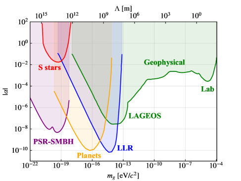
Figure 1: Constraints on the strength of the Yukawa interaction $\alpha$ at 95% C.L. as a function of the range of the Yukawa interaction $\Lambda$ from different experiments. The abscissa gives the mass of graviton via $m_{g}c^{2}=hc/\Lambda$. Different curves come from different experiments, and “PSR-SMBH” represents the constraints from an S2-like pulsar in Table 1. The curve of “S stars” represents the constraints from stars around Sgr A* [33]. The other curves come from Ref. [27].

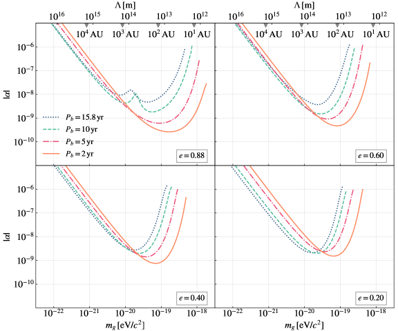
Figure 2: Constraints on the strength of the Yukawa interaction $\alpha$ at 68% C.L. from pulsars with different orbital periods and eccentricities. Different colored curves correspond to different orbital periods and different panels correspond to different eccentricities that are shown in the lower right corner. Other orbital parameters and observational information are the same as that in Table 1.

Besides the restrictions on $\alpha$ from an S2-like pulsar around Sgr A*, we also perform simulations with different orbital parameters. Figure 2 shows how the orbital period and eccentricity of pulsars influence the constraints on $\alpha$. Different colored curves correspond to different orbital periods, and different panels correspond to different eccentricities. For a selected system, the constraint on $\alpha$ usually becomes tightest when $\Lambda$ is close to the length scale of the system because, in this case, the Yukawa gravity has a significant deviation from the inverse-square law. A shorter orbital period corresponds to a smaller orbital semi-major axis, so the tightest bound on $\alpha$ will be obtained where $\Lambda$ is smaller. The orbtial eccentricity $e$ affects the range of distance covered by the system. A larger $e$ means that the distance between the pulsar and the SMBH varies more, so we can have decent bounds on $\alpha$ at a larger range of $\Lambda$. This corresponds to a wider pocket of the curves in Figure 2. In the figure, there are also potholes on curves from pulsars with high eccentricities and long orbital periods, caused by the absorption of residuals by the parameter $N_{0}$. As discussed earlier, when compared with short orbital period PSR-SMBH systems, within $T_{\rm obs}=20$ yr we can only observe one or two orbital periods for long orbital period PSR-SMBH systems, which means that the residuals from long orbital period PSR-SMBH systems may lack periodicity and become monotonous, and thus can be absorbed by the parameter $N_{0}$. Combined with the limited observational time, the absorption of the residuals by $N_{0}$ is more obvious for pulsars with high eccentricities. For pulsars with high eccentricities, the residuals caused by the Yukawa gravity will be mainly distributed at the part of periastron, showing a peak; for pulsars with low eccentricities, the residuals will be distributed across the orbital phases, showing a smooth curve. If the periastron of one orbital period is missed, for pulsars with high eccentricities, the residuals caused by the Yukawa gravity will be almost flat in that orbital period. But the absence of observation for the periastron has relatively little effects on pulsars with low eccentricities. So the absorption of the residuals by $N_{0}$ is more obvious for pulsars with high eccentricities.

3.2 Constraints on the range of the Yukawa interaction

In this subsection we limit the range of the Yukawa interaction $\Lambda$, which is related to the graviton mass $m_{g}$. The range of the Yukawa interaction $\Lambda$ corresponds to the Compton wavelength of the graviton, so the graviton mass can be expressed as [13, 14],

$$m_{g}c^{2}=\frac{hc}{\Lambda}\,,$$ (3.1)

where $h$ is the Planck constant. In GR, $m_{g}$ equals to zero and $\Lambda\to\infty$. The massive graviton will contribute an additional periastron advance rate, which is also the main source of timing residuals. Through the method of orbital perturbation [72], when the orbital semi-major axis $a_{\rm orb}\ll\Lambda$, the periastron advance from the Yukawa potential for each orbit can be expressed as [14],

$$\Delta\omega=\frac{\pi\alpha\sqrt{1-e^{2}}}{1+\alpha}\frac{a_{\rm orb}^{2}}{\Lambda^{2}}\,.$$ (3.2)

According to Eq. (3.2), when $\alpha$ changes from $\alpha=1$ to infinity, $\Delta\omega$ will only double. So with a given observational constraint on $\Delta\omega$, the limit on $1/\Lambda^{2}\sim m_{g}^{2}$ will change by the same amount. Therefore, here we fix $\alpha=1$ for an example. The limits on $m_{g}$ with another $\alpha$ can be easily estimated with Eq. (3.2). Now the set of parameters is $\bm{\Theta}^{(\alpha)}\equiv\bm{\Theta}\backslash\{\alpha\}=\{M,\ \nu,\ \dot{\nu},\ N_{0},\ e,\ P_{{b}},\ i,\ \omega,\ \varphi_{{\rm 0}},\ \Lambda\}$. GR can be recovered when the length scale $\Lambda$ tends to infinity, so we choose the fiducial value of $1/\Lambda$ to be zero, which means that we are limiting $m_{g}$ with a fiducial $m_{g}=0$. In the process of calculating the FIM, it is needed to calculate the first derivatives of $\mathcal{N}_{i}$ with respect to the model parameters. When $r\ll\Lambda$, the main effects on $\mathcal{N}_{i}$ by the Yukawa gravity are from the extra periastron advance (3.2) from the Yukawa potential. The extra periastron advance is proportional to $1/\Lambda^{2}$. If we take the derivative of $1/\Lambda$ and set $1/\Lambda$ to 0, this term will equal to zero and thus the first derivative of $\mathcal{N}_{i}$ with respect to $1/\Lambda$ will also equal to zero, which causes a situation where the FIM is approximately singular when the fiducial value for $1/\Lambda$ is zero. In this case, the FIM can not give the valid parameter estimation. So we adopt the DALI method to get the standard deviation of $m_{g}$. We use emcee [82] and corner [83] packages in our DALI calculation.

We consider limits on $m_{g}$ from a number of pulsars with different orbital periods and eccentricities. Other parameters of these pulsars and the observational information are the same as that in Table 1. The constraints on the graviton mass $m_{g}$ from different PSR-SMBH systems are shown in Figure 3. As we can see, the constraints on $m_{g}$ can be as small as $10^{-25}\,{\rm eV}/c^{2}$ at 68% C.L. from an S2-like pulsar. Compared with the bounds on $m_{g}$ from different experiments in Section 1, the limit from PSR-SMBH systems is more competitive, thanks to the high accuracy of pulsar timing technique. Besides, the PSR-SMBH systems are providing limits on the graviton mass in a strong-field regime. With the orbital semi-major axis, $a_{\rm orb}\propto P_{{b}}^{2/3}M^{1/3}$, we get the orbital period average for the periastron advance rate from the Yukawa gravity as $\dot{\omega}\equiv\Delta\omega/P_{{b}}\propto P_{{b}}^{1/3}M^{2/3}$ according to Eq. (3.2). Due to the huge mass of Sgr A* and the orbital periods of pulsars $P_{b}\gtrsim 1\,$yr under consideration, the rate of periastron advance will be significant. Overall, the PSR-SMBH systems provide an unrivalled opportunity to bound graviton mass.

In Figure 3, for pulsars with a same orbital eccentricity, a larger $P_{b}$ provides a tighter limit on $m_{g}$, which is a major trend according to the analysis of the periastron advance rate. But the curves do not show strict monotonicity because multiple factors affect the bounds on $m_{g}$. First, in the case of pulsar timing, given an observational span $T_{\rm obs}$, a larger $P_{b}$ means worse measurement accuracy of orbital parameters, which worsens the limit on $m_{g}$. Second, the absorption of residuals by the parameter $N_{0}$ will be significant for pulsars with long orbital periods and large eccentricities, which is detrimental to the bound. Finally, from the viewpoint of the actual observation, a larger $P_{b}$ is not always better for the constraint. For a pulsar with an extremely long $P_{b}$, it is difficult to cover one orbital period within the limited observational time, which leads to a looser bound on $m_{g}$. External perturbations will also be relevant, which are hard to model. For pulsars with both long orbital periods and high eccentricities, if we are unfortunate to miss the part of the periastron, the absence of that will greatly affect the bound. For pulsars with a same orbital period, the $m_{g}$ bound also depends on the eccentricity. According to Eq. (3.2), for a same $P_{b}$, the smaller the eccentricity is, the greater the advance of periastron is. At the same time, a small orbital eccentricity will reduce the measurement precision of the advance of periastron in pulsar timing. Combining these effects in our simulation, we finally get the results in Figure 3, showing the dependence of the $m_{g}$ bound on the orbital period and orbital eccentricity.

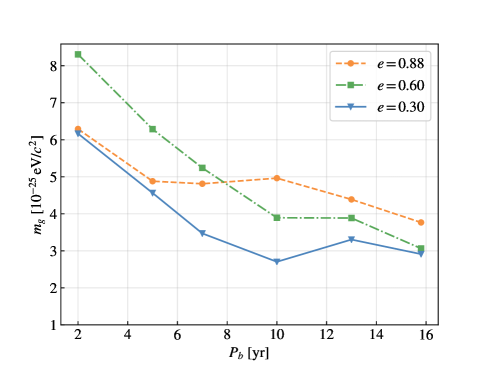
Figure 3: Constraints on the graviton mass at 68% C.L. with PSR-SMBH systems as a function of orbital period. Different color means different orbital eccentricities of pulsar orbits. Other orbital parameters and observational information are the same as that in Table 1.

In Figure 4 we show the posterior distribution of some parameters of an S2-like pulsar. The distortion in the ellipses in the posterior contours reflects the effects of higher order terms and the prior that $\Lambda>0$. Since the FIM can not give the valid posterior distribution, we have used the DALI method.

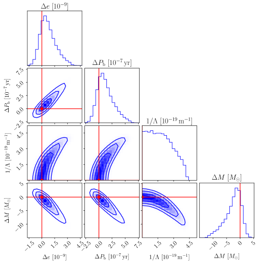
Figure 4: The posterior distribution of some parameters from the DALI method for an S2-like pulsar. The contours are drawn at the $1$-$\sigma$, $2$-$\sigma$ and $3$-$\sigma$ confidence levels. $\Delta e$ represents the difference between $e$ and its truth value in Table 1. $\Delta P_{{b}}$ and $\Delta M$ are given in the same way. Truth values of $\Delta e$, $\Delta P_{{b}}$, $\Delta M$, and $1/\Lambda$ are all zero and indicated as red lines.

3.3 Simultaneous bounds on $\alpha$ and $\Lambda$

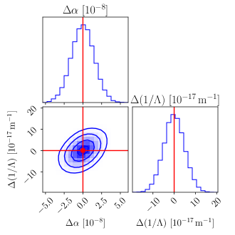
Figure 5: Distribution of parameter posteriors in the Yukawa gravity. The contours are drawn at the $1$-$\sigma$, $2$-$\sigma$ and $3$-$\sigma$ confidence levels. The distribution of posteriors is obtained by the DALI method. $\Delta\alpha$ and $\Delta(1/\Lambda)$ are the difference between parameters and their truth values, shown in Eq. (3.3). So the truth values of $\Delta\alpha$ and $\Delta(1/\Lambda)$ are zero and indicated as red lines.

In the above subsections, we have limited one of the Yukawa gravity parameters with the other one fixed. But if the Nature indeed follows the Yukawa gravity, i.e. $\alpha$ is non-zero and $\Lambda$ is finite, we need to limit both parameters simultaneously. However, there exist some difficulties to do so. If the length scale of system is much less than $\Lambda$, according to Eq. (3.2), the two parameters $\alpha$ and $\Lambda$ are highly degenerate. But if the length scale of the tested system is similar to $\Lambda$, we can detect higher order effects of $1/\Lambda$ and obtain decent limits on $\alpha$ and $\Lambda$ at the same time. So for a PSR-SMBH system with its length scale comparable to $\Lambda$, it is expected to break the degeneracy of $\alpha$ and $\Lambda$.

In this subsection, we test the ability of the PSR-SMBH system to measure $\alpha$ and $\Lambda$ simultaneously when the gravity is assumed to be the Yukawa gravity. We will calculate the standard deviations of $\alpha$ and $\Lambda$ simultaneously at fiducial values that $\alpha$ and $1/\Lambda$ are nonzero. In other words, we generate TOAs assuming that the gravity is the Yukawa gravity. Then we try to test whether we can measure $\alpha$ and $\Lambda$ simultaneously through a PSR-SMBH system. The set of parameters is $\bm{\Theta}=\{M,\ \nu,\ \dot{\nu},\ N_{0},\ e,\ P_{{b}},\ i,\ \omega,\ \varphi_{{\rm 0}},\ \alpha,\ \Lambda\}$. We adopt the DALI method to get more accurate parameter posteriors.

We choose an S2-like pulsar as an example, and the observational information is given in Table 1. We take one set of fiducial values of $\alpha$ and $\Lambda$ for illustration. The selection of fiducial values is based on the following considerations. First, we should be able to detect the deviation from the fiducial values, which means that we should choose the point above the curve of PSR-SMBH in Figure 1. Second, we would prefer that $\Lambda$ is similar to the orbital semi-major axis of an S2-like pulsar. We are more likely to break the degeneracy of $\alpha$ and $\Lambda$ in this case. Finally, we choose the fiducial values as,

$$\alpha =10^{-6}\,,$$ (3.3a)

$$1/\Lambda =10^{-14}\,{\rm m}^{-1}\,.$$ (3.3b)

Through parameter estimation on the simulated pulsar timing data, the distribution of two parameters of the Yukawa gravity is shown in Figure 5 using the DALI method. The posterior contours are almost elliptical with parameters in Eq. (3.3). We can prove that the posterior distributions are approximately Gaussian. From the figure, an S2-like PSR-SMBH system can give the following 1-$\sigma$ measurement uncertainties on the Yukawa gravity parameters,

$$\sigma_{\alpha} =1.5\times 10^{-8}\,,$$ (3.4a)

$$\sigma_{1/\Lambda} =4.8\times 10^{-17}\,{\rm m}^{-1}\,.$$ (3.4b)

As we can see, we have $\sigma_{\alpha}/\alpha=1.5\%$ and $\sigma_{1/\Lambda}/(1/\Lambda)=0.48\%$, which means that we can make a simultaneous measurement of $\alpha$ and $\Lambda$ in this artificially designed example. It demonstrates the prospects of PSR-SMBH systems measuring the Yukawa gravity parameters when the theory parameters happen to be optimal.

4 Conclusion and Outlook

In this paper, we discuss the test of the Yukawa gravity by timing a pulsar around Sgr A*. Considering an S2-like pulsar with 960 TOAs in a $20$-${\rm yr}$ observation, with an assumed realistic timing accuracy $\sigma_{\rm TOA}=100\,{\rm\mu s}$, we can expect to achieve the following.

1. When the range of the Yukawa interaction $\Lambda$ varies between $10^{1}$–$10^{4}\,{\rm AU}$, the constraints on the strength of the Yukawa interaction $|\alpha|$ will range between $10^{-8}$ and $10^{-6}$ (see Figure 1). Compared with other existing experiments, pulsars around Sgr A* will significantly shrink the parameter space of the Yukawa gravity in the region where $\Lambda=10^{1}$–$10^{4}\,{\rm AU}$.

2. By converting the range parameter into the graviton mass $m_{g}$, the upper limit on $m_{g}$ can reach as small as $10^{-25}\,{\rm eV}/c^{2}$, which is tighter than the results from the Solar system and observation of stars around Sgr A*.

3. If the gravity indeed follows the Yukawa gravity and $\Lambda$ is similar to the length scale of a PSR-SMBH system, it has the potential to break the degeneracy of the Yukawa gravity parameters, namely the strength parameter $\alpha$ and the range parameter $\Lambda$ simultaneously.

According to astrophysical estimates, it is likely to find a pulsar around Sgr A* by the SKA [63, 84, 64, 66]. Moreover, the assumed timing accuracy in this work, $\sigma_{\rm TOA}=100\,{\rm\mu s}$, is realistic for next-generation SKA-like telescopes [68], and the assumption that TOAs’ detection cadence is once per week is relatively conservative. In the future, it is promising to achieve the estimated accuracy in SKA-like projects if suitable pulsars around Sgr A* can be detected. Besides, a deeper understanding of the environment around Sgr A* will provide a more suitable PSR-SMBH timing model. We expect that we can detect useful pulsars around Sgr A* in the future, and promote gravity tests in the strong field in a profound way.

References

- Will [2014] C. M. Will, Living Rev. Rel. 17, 4 (2014), arXiv:1403.7377 [gr-qc] .
- Berti et al. [2015] E. Berti et al., Class. Quant. Grav. 32, 243001 (2015), arXiv:1501.07274 [gr-qc] .
- Bertone and Hooper [2018] G. Bertone and D. Hooper, Rev. Mod. Phys. 90, 045002 (2018), arXiv:1605.04909 [astro-ph.CO] .
- Debono and Smoot [2016] I. Debono and G. F. Smoot, Universe 2, 23 (2016), arXiv:1609.09781 [gr-qc] .
- Moffat [2004] J. W. Moffat, (2004), arXiv:astro-ph/0403266 .
- Saridakis et al. [2021] E. N. Saridakis, R. Lazkoz, V. Salzano, P. Vargas Moniz, S. Capozziello, J. Beltrán Jiménez, M. De Laurentis, and G. J. Olmo, eds., Modified Gravity and Cosmology (Springer, 2021).
- Hinterbichler [2012] K. Hinterbichler, Rev. Mod. Phys. 84, 671 (2012), arXiv:1105.3735 [hep-th] .
- van Dam and Veltman [1970] H. van Dam and M. J. G. Veltman, Nucl. Phys. B 22, 397 (1970).
- Zakharov [1970] V. I. Zakharov, JETP Lett. 12, 312 (1970).
- Vainshtein [1972] A. I. Vainshtein, Phys. Lett. B 39, 393 (1972).
- de Rham [2014] C. de Rham, Living Rev. Rel. 17, 7 (2014), arXiv:1401.4173 [hep-th] .
- Borka et al. [2013] D. Borka, P. Jovanović, V. B. Jovanović, and A. F. Zakharov, JCAP 11, 050 (2013), arXiv:1311.1404 [astro-ph.GA] .
- Zakharov et al. [2016] A. F. Zakharov, P. Jovanovic, D. Borka, and V. B. Jovanovic, JCAP 05, 045 (2016), arXiv:1605.00913 [gr-qc] .
- Zakharov et al. [2018] A. F. Zakharov, P. Jovanović, D. Borka, and V. Borka Jovanović, JCAP 04, 050 (2018), arXiv:1801.04679 [gr-qc] .
- Talmadge et al. [1988] C. Talmadge, J. P. Berthias, R. W. Hellings, and E. M. Standish, Phys. Rev. Lett. 61, 1159 (1988).
- Tsai et al. [2021] Y.-D. Tsai, Y. Wu, S. Vagnozzi, and L. Visinelli, (2021), arXiv:2107.04038 [hep-ph] .
- Cardone and Capozziello [2011] V. F. Cardone and S. Capozziello, Mon. Not. Roy. Astron. Soc. 414, 1301 (2011), arXiv:1102.0916 [astro-ph.CO] .
- Fischbach and Talmadge [1992] E. Fischbach and C. Talmadge, Nature 356, 207 (1992).
- Raffelt [1999] G. G. Raffelt, Ann. Rev. Nucl. Part. Sci. 49, 163 (1999), arXiv:hep-ph/9903472 .
- Adelberger et al. [2007] E. G. Adelberger, B. R. Heckel, S. A. Hoedl, C. D. Hoyle, D. J. Kapner, and A. Upadhye, Phys. Rev. Lett. 98, 131104 (2007), arXiv:hep-ph/0611223 .
- Niebauer et al. [1987] T. M. Niebauer, M. P. Mchugh, and J. E. Faller, Phys. Rev. Lett. 59, 609 (1987).
- Hoyle et al. [2001] C. D. Hoyle, U. Schmidt, B. R. Heckel, E. G. Adelberger, J. H. Gundlach, D. J. Kapner, and H. E. Swanson, Phys. Rev. Lett. 86, 1418 (2001), arXiv:hep-ph/0011014 .
- Adelberger et al. [2003] E. G. Adelberger, B. R. Heckel, and A. E. Nelson, Ann. Rev. Nucl. Part. Sci. 53, 77 (2003), arXiv:hep-ph/0307284 .
- Peron [2014] R. Peron, Adv. High Energy Phys. 2014, 791367 (2014).
- Williams et al. [2009] J. G. Williams, S. G. Turyshev, and D. H. Boggs, Int. J. Mod. Phys. D 18, 1129 (2009), arXiv:gr-qc/0507083 .
- Muller et al. [2008] J. Muller, J. G. Williams, and S. G. Turyshev, Astrophys. Space Sci. Libr. 349, 457 (2008), arXiv:gr-qc/0509114 .
- Konopliv et al. [2011] A. S. Konopliv, S. W. Asmar, W. M. Folkner, O. Karatekin, D. C. Nunes, S. E. Smrekar, C. F. Yoder, and M. T. Zuber, Icarus 211, 401 (2011).
- Hees et al. [2014] A. Hees, W. M. Folkner, R. A. Jacobson, and R. S. Park, Phys. Rev. D 89, 102002 (2014), arXiv:1402.6950 [gr-qc] .
- Li et al. [2014] Z.-W. Li, S.-F. Yuan, C. Lu, and Y. Xie, Res. Astron. Astrophys. 14, 139 (2014).
- Benisty [2022] D. Benisty, Phys. Rev. D 106, 043001 (2022), arXiv:2207.08235 [gr-qc] .
- Gillessen et al. [2009] S. Gillessen, F. Eisenhauer, S. Trippe, T. Alexander, R. Genzel, F. Martins, and T. Ott, Astrophys. J. 692, 1075 (2009), arXiv:0810.4674 [astro-ph] .
- Akiyama et al. [2022] K. Akiyama et al. (Event Horizon Telescope), Astrophys. J. Lett. 930, L12 (2022).
- Hees et al. [2017] A. Hees et al., Phys. Rev. Lett. 118, 211101 (2017), arXiv:1705.07902 [astro-ph.GA] .
- Bernus et al. [2019] L. Bernus, O. Minazzoli, A. Fienga, M. Gastineau, J. Laskar, and P. Deram, Phys. Rev. Lett. 123, 161103 (2019), arXiv:1901.04307 [gr-qc] .
- Will [2018] C. M. Will, Class. Quant. Grav. 35, 17LT01 (2018), arXiv:1805.10523 [gr-qc] .
- Jovanović et al. [2021] P. Jovanović, D. Borka, V. Borka Jovanović, and A. F. Zakharov, Eur. Phys. J. D 75, 145 (2021), arXiv:2105.03403 [astro-ph.GA] .
- de Rham et al. [2017] C. de Rham, J. T. Deskins, A. J. Tolley, and S.-Y. Zhou, Rev. Mod. Phys. 89, 025004 (2017), arXiv:1606.08462 [astro-ph.CO] .
- Bernus et al. [2020] L. Bernus, O. Minazzoli, A. Fienga, M. Gastineau, J. Laskar, P. Deram, and A. Di Ruscio, Phys. Rev. D 102, 021501 (2020), arXiv:2006.12304 [gr-qc] .
- Iorio [2007] L. Iorio, JHEP 10, 041 (2007), arXiv:0708.1080 [gr-qc] .
- Finn and Sutton [2002] L. S. Finn and P. J. Sutton, Phys. Rev. D 65, 044022 (2002), arXiv:gr-qc/0109049 .
- Miao et al. [2019] X. Miao, L. Shao, and B.-Q. Ma, Phys. Rev. D 99, 123015 (2019), arXiv:1905.12836 [astro-ph.CO] .
- de Rham et al. [2013] C. de Rham, A. J. Tolley, and D. H. Wesley, Phys. Rev. D 87, 044025 (2013), arXiv:1208.0580 [gr-qc] .
- Shao et al. [2020] L. Shao, N. Wex, and S.-Y. Zhou, Phys. Rev. D 102, 024069 (2020), arXiv:2007.04531 [gr-qc] .
- Will [1998] C. M. Will, Phys. Rev. D 57, 2061 (1998), arXiv:gr-qc/9709011 .
- Abbott et al. [2016] B. P. Abbott et al. (LIGO Scientific, Virgo), Phys. Rev. Lett. 116, 221101 (2016), [Erratum: Phys.Rev.Lett. 121, 129902 (2018)], arXiv:1602.03841 [gr-qc] .
- Abbott et al. [2021] R. Abbott et al. (LIGO Scientific, VIRGO, KAGRA), (2021), arXiv:2112.06861 [gr-qc] .
- Piórkowska-Kurpas [2022] A. Piórkowska-Kurpas, Universe 8, 83 (2022).
- Taylor [1992] J. H. Taylor, Phil. Trans. A. Math. Phys. Eng. Sci. 341, 117 (1992).
- Shao and Wex [2016] L. Shao and N. Wex, Sci. China Phys. Mech. Astron. 59, 699501 (2016), arXiv:1604.03662 [gr-qc] .
- Wex [2014] N. Wex, in Frontiers in Relativistic Celestial Mechanics: Applications and Experiments, Vol. 2, edited by S. M. Kopeikin (Walter de Gruyter GmbH, Berlin/Boston, 2014) p. 39, arXiv:1402.5594 [gr-qc] .
- Kramer [2016] M. Kramer, Int. J. Mod. Phys. D 25, 1630029 (2016), arXiv:1606.03843 [astro-ph.HE] .
- Miao et al. [2020] X. Miao, J. Zhao, L. Shao, N. Wex, M. Kramer, and B.-Q. Ma, Astrophys. J. 898, 69 (2020), arXiv:2006.09652 [gr-qc] .
- Shao [2022] L. Shao, (2022), arXiv:2206.15187 [gr-qc] .
- Shao and Yagi [2022] L. Shao and K. Yagi, Sci. Bull. 67, 1946 (2022), arXiv:2209.03351 [gr-qc] .
- Hulse and Taylor [1975] R. A. Hulse and J. H. Taylor, Astrophys. J. Lett. 195, L51 (1975).
- Taylor et al. [1979] J. H. Taylor, L. A. Fowler, and P. M. McCulloch, Nature 277, 437 (1979).
- Kramer et al. [2006] M. Kramer et al., Science 314, 97 (2006), arXiv:astro-ph/0609417 .
- Kramer et al. [2021] M. Kramer et al., Phys. Rev. X 11, 041050 (2021), arXiv:2112.06795 [astro-ph.HE] .
- Gillessen et al. [2017] S. Gillessen, P. M. Plewa, F. Eisenhauer, R. Sari, I. Waisberg, M. Habibi, O. Pfuhl, E. George, J. Dexter, S. von Fellenberg, T. Ott, and R. Genzel, Astrophys. J. 837, 30 (2017), arXiv:1611.09144 [astro-ph.GA] .
- Liu et al. [2021] K. Liu et al., Astrophys. J. 914, 30 (2021), arXiv:2104.08986 [astro-ph.HE] .
- Torne et al. [2021] P. Torne et al., Astron. Astrophys. 650, A95 (2021), arXiv:2103.16581 [astro-ph.HE] .
- Suresh et al. [2022] A. Suresh, J. M. Cordes, S. Chatterjee, V. Gajjar, K. I. Perez, A. P. V. Siemion, M. Lebofsky, D. H. E. MacMahon, and C. Ng, Astrophys. J. 933, 121 (2022), arXiv:2203.00036 [astro-ph.HE] .
- Cordes and Lazio [1997] J. M. Cordes and T. J. W. Lazio, Astrophys. J. 475, 557 (1997), arXiv:astro-ph/9608028 .
- Wharton et al. [2012] R. S. Wharton, S. Chatterjee, J. M. Cordes, J. S. Deneva, and T. J. W. Lazio, Astrophys. J. 753, 108 (2012), arXiv:1111.4216 [astro-ph.HE] .
- Zhang et al. [2014] F. Zhang, Y. Lu, and Q. Yu, Astrophys. J. 784, 106 (2014), arXiv:1402.2505 [astro-ph.GA] .
- Bower et al. [2018] G. C. Bower et al., ASP Conf. Ser. 517, 793 (2018), arXiv:1810.06623 [astro-ph.HE] .
- Bower et al. [2019] G. C. Bower et al., Bull. Am. Astron. Soc. 51, 438 (2019).
- Liu et al. [2012] K. Liu, N. Wex, M. Kramer, J. M. Cordes, and T. J. W. Lazio, Astrophys. J. 747, 1 (2012), arXiv:1112.2151 [astro-ph.HE] .
- Shao et al. [2015] L. Shao, I. Stairs, et al., PoS AASKA14, 042 (2015), arXiv:1501.00058 [astro-ph.HE] .
- Weltman et al. [2020] A. Weltman et al., Publ. Astron. Soc. Austral. 37, e002 (2020), arXiv:1810.02680 [astro-ph.CO] .
- Einstein et al. [1938] A. Einstein, L. Infeld, and B. Hoffmann, Annals Math. 39, 65 (1938).
- Poisson and Will [2014] E. Poisson and C. M. Will, Gravity (Cambridge, UK: Cambridge University Press, 2014).
- Blandford and Teukolsky [1976] R. Blandford and S. A. Teukolsky, Astrophys. J. 205, 580 (1976).
- Damour and Taylor [1992] T. Damour and J. H. Taylor, Phys. Rev. D 45, 1840 (1992).
- Wex and Kopeikin [1999] N. Wex and S. Kopeikin, Astrophys. J. 514, 388 (1999), arXiv:astro-ph/9811052 .
- Sellentin et al. [2014] E. Sellentin, M. Quartin, and L. Amendola, Mon. Not. Roy. Astron. Soc. 441, 1831 (2014), arXiv:1401.6892 [astro-ph.CO] .
- Wang et al. [2022] Z. Wang, C. Liu, J. Zhao, and L. Shao, Astrophys. J. 932, 102 (2022), arXiv:2203.02670 [gr-qc] .
- Hastings [1970] W. K. Hastings, Biometrika 57, 97 (1970).
- Skilling [2004] J. Skilling, AIP Conference Proceedings 735, 395 (2004).
- Skilling [2006] J. Skilling, Bayesian Analysis 1, 833 (2006).
- Liu et al. [2011] K. Liu, J. P. W. Verbiest, M. Kramer, B. W. Stappers, W. van Straten, and J. M. Cordes, Mon. Not. Roy. Astron. Soc. 417, 2916 (2011), arXiv:1107.3086 [astro-ph.HE] .
- Foreman-Mackey et al. [2013] D. Foreman-Mackey, D. W. Hogg, D. Lang, and J. Goodman, Publ. Astron. Soc. Pac. 125, 306 (2013), arXiv:1202.3665 [astro-ph.IM] .
- Foreman-Mackey [2016] D. Foreman-Mackey, The Journal of Open Source Software 1, 24 (2016).
- Smits et al. [2009] R. Smits, M. Kramer, B. Stappers, D. R. Lorimer, J. Cordes, and A. Faulkner, Astron. Astrophys. 493, 1161 (2009), arXiv:0811.0211 [astro-ph] .