Towards prediction of turbulent flows at high Reynolds numbers using high performance computing data and deep learning

Abstract

In this paper, deep learning (DL) methods are evaluated in the context of turbulent flows. Various generative adversarial networks (GANs) are discussed with respect to their suitability for understanding and modeling turbulence. Wasserstein GANs (WGANs) are then chosen to generate small-scale turbulence. Highly resolved direct numerical simulation (DNS) turbulent data is used for training the WGANs and the effect of network parameters, such as learning rate and loss function, is studied. Qualitatively good agreement between DNS input data and generated turbulent structures is shown. A quantitative statistical assessment of the predicted turbulent fields is performed.

1 Introduction

The turbulent motion of fluid flows is a complex, strongly non-linear, multi-scale phenomenon, which poses some of the most difficult and fundamental problems in classical physics. Turbulent flows are characterized by random spatio-temporal fluctuations over a wide range of scales. The general challenge of turbulence research is to predict the statistics of these fluctuating velocity and scalar fields. A precise prediction of these statistical properties of turbulence would be of practical importance for a wide field of applications ranging from geophysics to combustion science.

Research in the field of turbulence has mostly focused on a statistical description in the sense of Kolmogorov’s scaling theory. The theory proposed by Kolmogorov [10, 11] (known as K41 in literature) hypothesizes that for sufficiently large Reynolds numbers, small-scale motions are statistically independent from the large scales. While the large scales depend on the boundary or initial conditions, the smallest scales should be statistically universal and feature certain symmetries that are recovered in a statistical sense. Following Kolmogorov’s theory, the small scales can be uniquely described by simple parameters, such as the kinematic viscosity $\nu$ of the fluid and the mean dissipation rate $\langle{\varepsilon}\rangle$ (angular brackets denote ensemble-averaging). If the notion of small-scale universality was strictly valid, then there would be realistic hope for a statistical theory for turbulent flows. However, numerous experimental and numerical studies have reported a substantial deviation from Kolmogorov’s classical K41 prediction [3, 15], which is mostly due to internal intermittency. The consequence of internal intermittency is the break-down of small-scale universality, which dramatically complicates theoretical approaches from first principles.

In this work, a novel research route based on the method of deep learning (DL) is used to approach the challenge of turbulence modeling. In recent years, DL was improved substantially and has proven to be useful in a large variety of different fields, ranging from computer science to life science. However, to the knowledge of the authors, the application of DL to predict statistical behavior of small-scale turbulence is still new and many related issues are still unsolved. As described and despite its stochastic nature, turbulence exhibits certain coherent structures and statistical symmetries that are traceable by deep learning techniques. While analytical solutions exist for low-order correlation functions, for higher orders there is no such tractable solution available so far. Therefore, DL techniques are a promising approach to predict statistics of small-scale turbulence and an attempt to predict structures of turbulence is given here. Several DL networks from literature are tested by training them with high-fidelity direct numerical simulation (DNS) data of turbulence. The predicted turbulence data is evaluated by qualitative and quantitative comparisons with the original data and the statistics of the original data, respectively. As one challenge in the application of DL is to find optimal network architectures and hyperparameters, several combinations were evaluated for this work.

The remainder of this paper is organized as follows. In Sec. 2, future chances and challenges of DL in the context of turbulence are summarized. Then, the used DNS data base is described in Sec. 3. Section 4 presents results in terms of predicted turbulent structures and discusses the sensitivity of the results with respect to network parameters, such as learning rate and loss function. The paper finishes with conclusions in Sec. 5.

2 Deep Learning and Turbulence

The Reynolds number is the most important parameter for characterizing turbulent flows. It can be defined as the ratio of the size of the large vortices to the size of the smallest vorticies and can be understood as a measure for the scale separation [13]. Thus, it also plays a central role in any attempt to model turbulence accurately and must be considered in the DL network. As the application of DL for predicting turbulence is new, the following steps need to be taken on the way to find a turbulence model based on DL:

1. A posteriori analysis with fixed Reynolds number: The ability of certain network types to predict statistics of turbulence needs to be evaluated. Therefore, the Reynolds number should be fixed and unsupervised learning can be performed. The accuracy of the trained DL networks can be evaluated by comparison with the original data and corresponding statistics. The ability to predict statistics for a given Reynolds number is essential for an improved understanding of universality and intermittency as well as for the development of models.

2. A posteriori analysis with flexible Reynolds numbers: As a next step, DL should be used with flexible Reynolds numbers. A combination of unsupervised and supervised DL can be employed to improve the understanding of the universality of turbulence. For example, it will be interesting to see whether a DL network, which was trained within a certain range of Reynolds numbers, is able to also predict turbulent structures for higher Reynolds numbers correctly.

3. A priori analysis: Also, DL can be used to identify characteristic structures of the turbulent dissipation field by a pattern recognition technique. Relevant quantities under consideration should be the moments of the dissipation $M_{n}$, the kinetic energy, and two-point correlation functions or structure functions of the velocity field.

4. Modeling of small-scale turbulence: For many fields in turbulence research, small-scale quantities are not known, either due to modeling of the small scales in numerical approaches or due to lack of resolution in experimental techniques. For reduced order models of turbulence, it is required to be able to predict statistics of the dissipation without knowing the actual dissipation field. The goal is to develop a DL network that is able to predict statistics of the fine-scale motion by knowing the exact velocity field from DNS or a coarse-grained velocity field only. The reliability of the neural network can be statistically evaluated against data from DNS, keeping in mind that neural networks can fail under certain conditions.

3 DNS Data Base

The application of DL is only possible if a sufficiently large and accurate data base exists. In recent years, a comprehensive data base of DNSs has been created based on some of the world’s largest turbulence simulations [6, 5, 12, 4] using high performance computing (HPC). The data base contains different flow setups, such as forced homogeneous isotropic turbulence as well as free shear flows, and the data sets are freely available from the corresponding author upon request. DNS solves the governing equations of turbulence (namely the Navier-Stokes equations) numerically for all relevant scales, without relying on any turbulence models. Due to internal intermittency, turbulent flows reveal a hierarchy of viscous cut-off scales [2] and the computation of higher-order statistics of small-scale quantities requires a spatial resolution that may be finer than the Kolmogorov length scale. DNS has become an indispensable tool in the field of turbulence research as it provides accurate access to three-dimensional (3-D) fields under controlled conditions.

Characteristic properties of the DNSs are listed in Table 1. $N$ denotes the number of grid points, ${\rm Re}_{\lambda}$ is the Reynolds number based on the Taylor micro-scale, $\kappa_{\rm max}$ is the largest resolved wave-number, $\eta$ is the Kolmogorov length scale, $\langle{\varepsilon}\rangle$ is the mean energy dissipation. $M$ denotes the number of statistically independent boxes being available.

Table 1: Characteristic parameters of the DNS data base. The DNS data base is used to train and test the neural network.

	S	R0	R1	R2	R3	R4	R5	R6
$N$	$1024\times 512\times 512\;$	$512^{3}$	$1024^{3}$	$1024^{3}$	$2048^{3}$	$2048^{3}$	$4096^{3}$	$4096^{3}$
${\rm Re}_{\lambda}$	$\approx 50$	88	119	184	215	331	529	754
$\nu$	-	0.01	0.0055	0.0025	0.0019	0.0010	0.00048	0.00027
$\kappa_{\rm max}\eta$	$>2.5$	3.93	4.99	2.93	4.41	2.53	2.95	1.60
$M$	1	189	62	61	10	10	10	11

Training of the DL is performed based on a passive scalar $\phi$ which is transported by an advection-diffusion equation. The passive scalar represents the dynamical motion of turbulence and its prediction by DL is of fundamental relevance for the modeling of turbulence. Figure 1 displays a visualization of the instantaneous scalar $\phi$ and the scalar dissipation rate $\chi$ for case R5. The scalar dissipation rate is defined as

$$\chi=2D\left(\nabla\phi\right)^{2}$$ (1)

and signifies the destruction of scalar fluctuations due to molecular diffusivity $D$. The scalar field reveals distinct coherent regions of roughly constant scalar values. The size of these regions is of the order of the scalar integral length scale and they are separated by sharp highly convoluted boundaries. At these boundaries, the scalar dissipation rate attains large values. As a consequence, the scalar dissipation rate is characterized by filamented structures representing a high level of intermittency.

(a) Scalar field

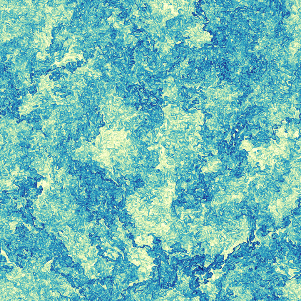
(b) Scalar dissipation rate field

Figure 1: Visualization of the instantaneous fields of the scalar $\phi$ and the scalar dissipation rate $\chi$ for case R5.

4 Results

A first step towards the development of universal turbulent models based on DL is to study the ability of networks to generate small-scale turbulent structures. For that, slice-wise training of certain DL networks with the DNS data at fixed Reynolds number was performed. More precisely, the 3-D scalar fields $\phi$ of the DNS data are cut into 2-D slices, which are statistically similar. The distance between two adjacent slices is chosen large enough to ensure that structures are uncorrelated. The 2-D slices are used as input for the training of the network, which is able to reproduce these structures as output in the end. For this reproduction of turbulent structures, 100 random values following a normal Gaussian distribution with zero-mean and a standard deviation, which is linearly mapped between 0 and 1 by the local Reynolds number, are considered as input data. The implementation was done using Keras/TensorFlow/Horovod and the training was performed on JURECA, a supercomputer at JSC, FZ Jülich featuring two NVIDIA Tesla K80 GPUs with a dual-GPU design on each used computing node.

More precisely, for this work, generative adversarial networks (GAN) [7], which use an adversarial game between generator and discriminator to optimize the network, were evaluated regarding their suitability to generate small-scale turbulence. Furthermore, Wasserstein GANs (WGANs) [1] featuring advantages in terms of stability and good interpretability of the learning curve as well as u-net [14], consisting of a contracting path to capture context and a symmetric expanding path that enables precise localization, were tried.

A visualization of one arbitrary input slice cut from the DNS data and one arbitrary output slice predicted by the DL networks for case S is shown in Fig. 2. The WGAN gives the best results and is able to reproduce coherent motions and small-scale structures, which are characteristic for fluid turbulence. GAN and u-net have problems especially to reproduce regions without any fluctuations and always feature some noise. Due to these results, the WGAN was tested in more detail and quantitative results based on statistics in the original and predicted data are presented in the following.

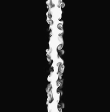
(a) DNS (original)

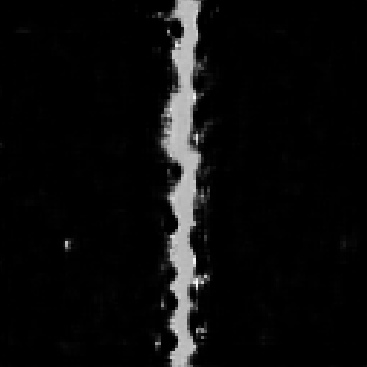
(b) GAN (generated)

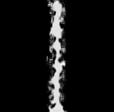
(c) WGAN (generated)

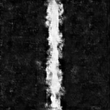
(d) u-net (generated)

Figure 2: Comparison of an arbitrary DNS data slice of the passive scalar $\phi$ and comparison with data generated by various DL networks.

As briefly mentioned in the beginning, one main challenge in the context of DL is to find suitable network architectures and hyperparameters resulting in an accurate solution. For the considered turbulence, a WGAN made of four layers for the discriminator and three layers for the generator gave good results. Each discriminator-layer contained a convolution (Conv2D, kernel_size=3, striding=2 or 1), an activiation (LeakyReLU, alpha=0.2), and a dropout (Dropout). Partly, zero-padding (ZeroPadding), batch normalization (BatchNormalization, momentum=0.8), and flattening (Flatten) were employed. Each generator-layer used a convolution (Conv2D, kernel_size=4) and batch normalization (BatchNormalization(momentum=0.8) in combination with either tanh- or relu-activation.

A more rigorous quantitative analysis of the generated small-scale turbulence is shown in Figs. 3 and 4. It gives the resulting normalized mean ($\langle{\phi}\rangle^{*}$) and variance profile ($\langle{{\phi}^{\prime 2}}\rangle^{*}$) of the scalar for different learning rates $l_{\mathrm{r}}$ as function of the non-dimensional cross-stream direction $y/H_{0}$. The maximum values are normalized to 1, $H_{0}$ is the initial jet width, and the asterisk indicates a normalized quantity. Furthermore, the scalar fluctuation is defined as ${\phi}^{\prime}=\phi-\langle{\phi}\rangle$. It can be seen that the network is able to generate structures with the correct statistical properties as long as a proper learning rate is chosen. A too small value for the learning rate leads to non-converged results, while a too high value gives noise.

(a) $l_{\mathrm{r}}=0.00001$

(b) $l_{\mathrm{r}}=0.0000005$

(c) $l_{\mathrm{r}}=0.00000001$

Figure 3: Comparison of the normalized scalar mean profile $\langle{\phi}\rangle^{*}$ for case S for different learning rates $l_{\mathrm{r}}$ plotted as function of the non-dimensional cross-stream direction $y/H_{0}$.

(a) $l_{\mathrm{r}}=0.00001$

(b) $l_{\mathrm{r}}=0.0000005$

(c) $l_{\mathrm{r}}=0.00000001$

Figure 4: Comparison of the normalized scalar variance $\langle{{\phi}^{\prime 2}}\rangle^{*}$ for case S for different learning rates $l_{\mathrm{r}}$ as function of the non-dimensional cross-stream direction $y/H_{0}$.

Finally, the DL approach is evaluated by means of two-point statistics. Turbulence is a non-local, multi-scale problem that is characterized by a transfer of turbulent energy from the large scales to the smaller scales, where the energy is dissipated due to molecular viscosity. Therefore, a two-point description of turbulence is customary as it captures both local and non-local phenomena. The two-point correlation function of the scalar field, defined as

$$f_{\phi}(\underline{r};\underline{x},t)=\langle{{\phi}^{\prime}(\underline{x}+\underline{r};t){\phi}^{\prime}(\underline{x};t)}\rangle$$ (2)

with underlines indicating vectors, is a statistical quantity of prime importance and measures how the scalar field at the two independent points $\underline{x}+\underline{r}$ and $\underline{x}$ is correlated. If the two points are statistically independent then $f(\underline{r};\underline{x},t)=0$. The normalized correlation function of the scalar field, given by

$$f_{\phi}^{*}(\underline{r};\underline{x},t)=\frac{\langle{{\phi}^{\prime}(\underline{x}+\underline{r};t){\phi}^{\prime}(\underline{x};t)}\rangle}{\langle{{\phi}^{\prime 2}}\rangle},$$ (3)

is shown in Fig. 5 for the DNS data and for the data obtained by DL evaluated at the center-plane in spanwise direction $z$ for a single timestep. A good agreement between the normalized correlation functions can be observed signifying that the DL approach is able to reproduce the local structure of turbulence with high accuracy. Different statistical quantities, such as the integral length scale $l_{\mathrm{t}}$, the scalar variance $\langle{{\phi}^{\prime 2}}\rangle$, and the averaged scalar dissipation rate $\langle{\chi}\rangle$, can be computed from the correlation function. In other words, the ability to predict the correlation function correctly is a first step towards building a model for turbulence (cf. [9]).

Figure 5: Normalized scalar correlation function $f_{\phi}^{*}$ for case S as function of the non-dimensional separation distance in spanwise direction $r_{z}/H_{0}$. The correlation function is computed at the center-plane for learning rate $l_{\mathrm{r}}=0.0000005$.

5 Conclusions

In this work, DL is applied to turbulent fields obtained from DNS. The effect of various network and training parameters, such as learning rate and loss function, are discussed. Using WGANs, it was possible to generate small-scale turbulence which features the same structures as observed in DNS data. A comparison of the statistics evaluated on the original and predicted data showed promising agreement. This is an important first step towards the prediction of turbulent flows at various Reynolds numbers. As a next step, the ability of the trained network to generate turbulent structures for various given Reynolds numbers will be evaluated.

References

- [1] Arjovsky, M., Chintala, S., Bottou, L.: Wasserstein GAN. arXiv:1701.07875v3 (2017)
- [2] Boschung, J., Hennig, F., Gauding, M., Pitsch, H., Peters, N.: Generalised higher-order kolmogorov scales. Journal of Fluid Mechanics 794, 233–251 (2016)
- [3] Frisch, U.: Turbulence - The legacy of A.N. Kolmogorov. Cambridge University Press, Cambridge, UK (1995)
- [4] Gauding, M., Danaila, L., Varea, E.: High-order structure functions for passive scalar fed by a mean gradient. International Journal of Heat and Fluid Flow 67, 86–93 (2017)
- [5] Gauding, M., Goebbert, J.H., Hasse, C., Peters, N.: Line segments in homogeneous scalar turbulence. Physics of Fluids 27(9), 095102 (2015)
- [6] Gauding, M., Wick, A., Peters, N., Pitsch, H.: Generalized scale-by-scale energy budget equations for large-eddy simulations of scalar turbulence at various Schmidt numbers. Journal of Turbulence (2013)
- [7] Goodfellow, I.J., Pouget-Agadie, J., Mirza, M., Xu, B., Warde-Farley, D., Ozair, S., Courville, A., Bengio, Y.: Generative Adversarial Networks. arXiv:1406.2661 (2014)
- [8] Jülich Supercomputing Centre: JUQUEEN: IBM Blue Gene/Q Supercomputer system at the Jülich supercomputing centre. Journal of large-scale research facilities 1 (2015)
- [9] von Karman, T., Howarth, L.: On the statistical theory of isotropic turbulence. Proceedings of the Royal Society of London A: Mathematical, Physical and Engineering Sciences 164(917), 192–215 (1938)
- [10] Kolmogorov, A.N.: Dissipation of energy in locally isotropic turbulence. In: Dokl. Akad. Nauk SSSR. vol. 32, pp. 16–18 (1941)
- [11] Kolmogorov, A.N.: The local structure of turbulence in incompressible viscous fluid for very large reynolds numbers. In: Dokl. Akad. Nauk SSSR. vol. 30, pp. 299–303 (1941)
- [12] Peters, N., Boschung, J., Gauding, M., Goebbert, J.H., Hill, R.J., Pitsch, H.: Higher-order dissipation in the theory of homogeneous isotropic turbulence. Journal of Fluid Mechanics 803, 250–274 (2016)
- [13] Pope, S.B.: Turbulent flows. Cambridge University Press, Cambridge, UK (2000)
- [14] Ronneberger, O., Fischer, P., Brox, T.: U-Net: Convolutional Networks for Biomedical Image Segmentation. arXiv:1505.04597 (2015)
- [15] Sreenivasan, K.R.: The passive scalar spectrum and the Obukhov-Corrsin constant. Physics of Fluids 8, 189 (1996)