Spin and charge modulations of a half-filled extended Hubbard model

Abstract

We introduce and analyze an extended Hubbard model, in which intersite Coulomb interaction as well as a staggered local potential (SLP) are considered, on the square lattice at half band filling, in the thermodynamic limit. Using both Hartree-Fock approximation and Kotliar and Ruckenstein slave boson formalism, we show that the model harbors charge order (CO) as well as joint spin and charge modulations (SCO) at finite values of the SLP, while the spin density wave (SDW) is stabilized for vanishing SLP, only. We determine their phase boundaries and the variations of the order parameters in dependence on the SLP, as well as on the on-site and nearest-neighbor interactions. Domains of coexistence of CO and SCO phases, suitable for resistive switching experiments, are unraveled. We show that the novel SCO systematically turns into the more conventional SDW phase when the zero-SLP limit is taken. We also discuss the nature of the different phase transitions, both at zero and finite temperature. In the former case, no continuous CO to SDW (or SCO) phase transition occurs. In contrast, a paramagnetic phase (PM), which is accompanied with continuous phase transitions towards both spin or charge ordered phases, sets in at finite temperature. A good quantitative agreement with numerical simulations is demonstrated, and a comparison between the two used approaches is performed.

I Introduction

Electronic phases displaying spin and charge modulations are currently undergoing intense scrutiny Wu et al. (2021); Campi et al. (2022). Following the seminal works by Tranquada et al. on doped nickelatesTranquada et al. (1994); Sachan et al. (1995), they are firstly found in doped Mott insulators. They received even stronger interest when related order was evidenced in the superconducting Sr-doped La₂CuO₄ cuprates (LSCO) Tranquada et al. (1995). Furthermore, striped states have been exhibited in other series of oxides as well which, most notably, include layered cobaltates Cwik et al. (2009) and layered manganites Ulbrich and Braden (2012), as reviewed in, e. g., Ref. [Ulbrich and Braden, 2012].

A diversity of stripe orders have been reported. Indeed, the wave-vectors characterizing the modulations may either lie along the diagonal of the Brillouin zone (BZ), in which case the stripe is coined diagonal, or along the side of the BZ, and the stripe is said to be vertical. The stripes observed in nickelates are diagonal and are systematically found to be insulating Cheong et al. (1994); Hücker et al. (2007). This holds true for layered cobaltates and layered manganites as well. Cuprates, in contrast, present both diagonal and vertical stripes, with the former being insulating and the latter metallic, if not superconductingHücker et al. (2011). Explaining the insulating nature of La_2-xSr_xNiO₄ nickelates by Density Functional Theory, including optimized lattice distortion Yamamoto et al. (2007); Schwingenschlögl et al. (2008, 2009), or by means of model calculations Raczkowski et al. (2006a), turned out to be challenging. Conversely, for cuprates, a systematics of insulating diagonal filled (with nearly 1 hole per domain wall) and metallic half-filled (with nearly 0.5 hole per domain wall) stripes could be established within model calculations Raczkowski et al. (2006b). More recent numerical calculations applying a variety of approaches tackled the issue of d-wave superconductivity in the ground state of the two-dimensional Hubbard Model. As of today, it appears fair to say that it could not unambiguously be established. Actually, stripe order has been found to be very close, if not lower, in energy to its superconducting counterpart Himeda et al. (2002); Ido et al. (2018); White and Scalapino (2009); Huang et al. (2018); Corboz et al. (2014); Ponsioen et al. (2019); Li et al. (2021) — coexistence of both phases has been highlighted too Leprévost et al. (2015); Jiang et al. (2020) albeit not necessarily in the ground state Zheng et al. (2017).

So far we briefly presented spin and charge modulated phases of the doped two-dimensional Hubbard model, but would they persist in the half band filling limit? No positive answer to this question resulted from the study of the two-dimensional Hubbard model which, for repulsive on-site interaction $U>0$, only harbors antiferromagnetism. This could be presumed considering the following qualitative picture of the stripe modulations. The spatial periods of the charge order in the striped phase are bounded by holes, or fractions of holes. A higher hole concentration thus eventually leads to a shorter spatial period of the stripe ordering, and conversely. By taking the limit where the hole doping tends to zero, the period of the stripe order diverges such that we are left with the usual antiferromagnetic Mott insulating phase at half band-filling. This heuristic argument supports the assumption that the mechanisms underlying spin-and-charge modulations at half filling should differ from those underlying the striped phases at finite doping. Additionally, evidence of the existence of a spin-and-charge ordered phase in the half-filled Hubbard model remains elusive van Dongen (1994a, b); Wolff (1983); Deeg et al. (1993); Hirsch (1984); Sengupta et al. (2002); Zhang and Callaway (1989); Terletska et al. (2017); Paki et al. (2019). As a consequence to this, in the present work, a Hubbard model extended with a nearest-neighbor interaction term of intensity $V$ as well as a spatial modulation of the energy levels $\varepsilon_{\rm i}$ in order to straightforwardly induce charge order in the antiferromagnetic phase is considered, and phases bridging between pure magnetic order and pure charge order are sought for.

The rich landscape of competing electronic phases displayed by metal oxides is not their only point of interest. When the transition between different states is of the first order, it can be harnessed for application in digital electronics. Since the functionnal materials can keep their valuable properties down to the nanoscale, they promise to offer a superior alternative to conventional semiconductor components Takagi and Hwang (2010); Coll et al. (2019). In particular, resistive switching in Mott systems is the subject of intense investigations, since it could enable a variety of novel functions, such as resistive RAM for data storage Janod et al. (2015); Wang et al. (2019), optoelectronics Liao et al. (2018); Coll et al. (2019), or neuromorphic computing Del Valle et al. (2018, 2019); Bauers et al. (2021). Their switch between resistivity values which may differ by several orders of magnitude, can be experimentally triggered by varying different control parameters, such as chemical doping, strain, temperature, hydrostatic pressure, electric field, current, and illumination. The microscopic mechanisms that drive the phase transition are, however, still debated Diener et al. (2018); Kalcheim et al. (2020); Babich et al. (2022); Adda et al. (2022). Yet the diversity of stimuli indicates that several are likely at play depending on the material, and it highlights the versatility of the phenomenon as a tool for future technologies.

In this context, we analyze our model by performing both Hartree-Fock (HF) and Kotliar-Ruckenstein slave boson (KRSB) slave boson calculations. While the former method mostly yields qualitative understanding, the latter better incorporates correlation effects.

This paper is organized as follows: in Sec. II the considered Hamiltonian, the HF approximation as well as the saddle-point approximation to the KRSB representation used in this study are presented. In Sec. III within the HF approximation, and in Sec. IV within the KRSB representation, the zero-temperature phase diagram of the half-filled model on the square lattice is unraveled for different values of the splitting $\varepsilon$ and a novel spin-and-charge ordered phase is presented. In Sec. V, within the KRSB representation, the $\varepsilon=0$ limit is taken in order to recover the $t$–$U$–$V$ model and the phase diagram is presented for zero and finite temperature. We then compare, in Sec. VI, the results obtained within both formalisms in order to assess for the relevance of electronic correlations in the presented phases. Finally, Sec. VII presents conclusions and a short outlook. Appendix A details the self-consistent field equations to be solved in the HF approximation. Appendix B gives more details about the setup of the different saddle-points, together with the derivation of the saddle-point equations.

II Model and methods

II.1 Extended Hubbard model

Initially introduced nearly simultaneously by Hubbard Hubbard and Flowers (1963), Kanamori Kanamori (1963) and Gutzwiller Gutzwiller (1963) as a model for electrons in transition-metal oxides, the now-called Hubbard model is the archetype of correlated electrons model. Its Hamiltonian embodies the competition between kinetic energy and Coulomb interactions in its simplest form. It reads

$$\mathcal{H}_{\rm Hub}=\mathcal{H}_{\rm 0}+\mathcal{H}_{\rm U},$$ (1)

with the one-body part, in the grand canonical ensemble,

$$\mathcal{H}_{\rm 0}=\sum_{\rm i,j,\sigma}t^{\rm\phantom{0}}_{\rm ij}c^{\dagger}_{\rm i,\sigma}c^{{\vphantom{\dagger}}}_{\rm j,\sigma}-\mu\sum_{\rm i,\sigma}c^{\dagger}_{\rm i,\sigma}c^{{\vphantom{\dagger}}}_{\rm i,\sigma},$$ (2)

and the local interaction term

$$\mathcal{H}_{\rm U}=U\sum_{\rm i}c^{\dagger}_{\rm i,\uparrow}c^{\dagger}_{\rm i,\downarrow}c^{{\vphantom{\dagger}}}_{\rm i,\downarrow}c^{{\vphantom{\dagger}}}_{\rm i,\uparrow},$$ (3)

where $c^{\dagger}_{\rm i,\sigma}$ ($c^{{\vphantom{\dagger}}}_{\rm i,\sigma}$) creates (annihilates) an electron with spin $\sigma\in\{\uparrow,\downarrow\}$ at the lattice site i, $n_{\rm i,\sigma}$ is the usual electron number operator ($n_{\rm i}=n_{\rm i,\uparrow}+n_{\rm i,\downarrow}$), $t^{\rm\phantom{0}}_{\rm ij}$ is the hopping amplitude between lattice sites i and j, $\mu$ is the chemical potential controlling the band filling and $U$ is the on-site Coulomb interaction strength. Nevertheless, Hubbard himself pointed out the major drawback of his model when it comes to faithfully describing the microscopic processes happening in real systems, namely the over-simplified treatment of the Coulomb interaction Hubbard and Flowers (1964). In cuprates, for example, it appears that the screening of the Coulomb interaction between electrons is not perfect and thus yields inter-atomic contributions. As a response to this, longer-ranged Coulomb interactions may be incorporated in the Hamiltonian, yielding the additional term

$$\mathcal{H}_{\rm V}=\frac{1}{2}\sum_{\rm\begin{subarray}{c}\rm i,j\\ \sigma,\sigma^{\prime}\end{subarray}}V_{\rm ij}c^{\dagger}_{\rm i,\sigma}c^{\dagger}_{\rm j,\sigma^{\prime}}c^{{\vphantom{\dagger}}}_{\rm j,\sigma^{\prime}}c^{{\vphantom{\dagger}}}_{\rm i,\sigma},$$ (4)

where $V_{\rm ij}$ is the Coulomb coupling between sites i and j. The $1/2$ factor accounts for the double-counting of the $\rm(i,j)\equiv(j,i)$ pairs in the sum. Henceforth, we assume the screening of the long-ranged Coulomb interaction to be efficient, and we choose $V_{\rm ij}$ such that $V_{\rm ij}=V$ if i and j are nearest-neighbors and $V_{\rm ij}=0$ otherwise. Approximating the Coulomb interaction in such a way yields the often-called extended or $t$–$U$–$V$ Hubbard model

$$\mathcal{H}_{\rm t-U-V}=\mathcal{H}_{\rm Hub}+\mathcal{H}_{\rm V}.$$ (5)

Turning next to our search for a minimal model of spin-and-charge modulated phases at half-filling, we propose to further extend the $t$–$U$–$V$ model by also considering an staggered local potential (SLP) of the form

$$\mathcal{H}_{\rm\varepsilon}=\sum_{\rm i,\sigma}\varepsilon_{\rm i}c^{\dagger}_{\rm i,\sigma}c^{{\vphantom{\dagger}}}_{\rm i,\sigma}.$$ (6)

This potential either arises from an inhomogeneous crystal field inside a material or an alternating intensity of the confinement potential in the context of cold fermions on an optical lattice. Models of strong disorder, where $\varepsilon_{\rm i}$ is randomly distributed across the lattice such that each site has a different electrostatic environment, has been considered in the context of many-body localization Žnidarič et al. (2008); Prelovšek et al. (2021). In the present case however, the focus is made on minimal extensions to the Hubbard model. We thus consider the simple form

$$\varepsilon_{\rm i}=-\varepsilon\quad\text{if}\quad\rm i\in A,$$ (7a)

$$\varepsilon_{\rm i}=+\varepsilon\quad\text{if}\quad\rm i\in B,$$ (7b)

where A and B are the two sublattices of a bipartite lattice. In the context of LSCO superconductors, alternating La and, e. g., Pr chains, could produce such a contribution to the crystal field, as the electronic cloud of the La cations is more extended than the one of the Pr cations. This results in a staggered $2\varepsilon$ energy distribution between adjacent lattice sites. This finally leads us to the Hamiltonian

$$\mathcal{H}_{\rm ext}=\mathcal{H}_{\rm Hub}+\mathcal{H}_{\rm V}+\mathcal{H}_{\rm\varepsilon},$$ (8)

which will be investigated in Sec. III and in Sec. IV.

Throughout the present study, we work in the half-filled subspace of the square lattice, such that

$$\sum_{\rm i,\sigma}\langle n_{\rm i,\sigma}\rangle=N_{\rm L},$$ (9)

where $N_{\rm L}$ is the total number of lattice sites and we set the lattice parameter $a=1$ thereby fixing the length scale.

II.2 HF approximation

Throughout this work, we use the HF approximation as a benchmark for the weak coupling regime and compare its results in the intermediate-to-strong coupling regime with the KRSB results including correlations. In this framework, the interaction terms in Eq. (5) are approximated by

$$\mathcal{H}_{\rm U}\approx U\sum_{\rm i,\sigma}\left(\langle n_{\rm i,-\sigma}\rangle c^{\dagger}_{\rm i,\sigma}c^{{\vphantom{\dagger}}}_{\rm i,\sigma}-\frac{1}{2}\langle n_{\rm i,\uparrow}\rangle\langle n_{\rm i,\downarrow}\rangle\right),$$ (10)

and

$$\mathcal{H}_{\rm V}\approx V\sum_{\rm\langle ij\rangle,\sigma} \left[\sum_{\rm\sigma^{\prime}}\left(\langle n_{\rm j,\sigma^{\prime}}\rangle c^{\dagger}_{\rm i,\sigma}c^{{\vphantom{\dagger}}}_{\rm i,\sigma}-\frac{1}{2}\langle n_{\rm i,\sigma}\rangle\langle n_{\rm j,\sigma^{\prime}}\rangle\right)\right.$$

$$\left.-\frac{1}{2}\langle b_{\rm ij,\sigma}\rangle\left(c^{\dagger}_{\rm i,\sigma}c^{{\vphantom{\dagger}}}_{\rm j,\sigma}+\rm{h.c.}\right)+\frac{1}{2}\langle b_{\rm ij,\sigma}\rangle^{\rm 2}\right],$$ (11)

where

$$\langle n_{\rm i,\sigma}\rangle=\langle c^{\dagger}_{\rm i,\sigma}c^{{\vphantom{\dagger}}}_{\rm i,\sigma}\rangle,$$ (12a)

$$\langle n_{\rm i}\rangle=\langle n_{\rm i,\uparrow}\rangle+\langle n_{\rm i,\downarrow}\rangle,$$ (12b)

$$\langle b_{\rm ij,\sigma}\rangle=\langle c^{\dagger}_{\rm i,\sigma}c^{{\vphantom{\dagger}}}_{\rm j,\sigma}\rangle,$$ (12c)

and the $\langle ij\rangle$ summation denotes a sum over nearest-neighbors in which both the $(i,j)$ and $(j,i)$ bonds are counted.

In this work, we investigate spin and/or charge ordered phases at half band filling. Such phases are described by mean fields of the form

$$\langle n_{\rm i,\sigma}\rangle=\frac{1}{2}+\delta n_{\rm\sigma}\exp(\mathrm{i}\textbf{Q}\cdot\textbf{R}_{\rm i}),$$ (13a)

$$\delta n_{\rm\sigma}=\frac{1}{2}\left(\delta n+\underline{\tau}^{\rm 3}_{\rm\sigma\sigma}m_{\rm z}\right),$$ (13b)

$$\langle b_{\rm ij,\sigma}\rangle=b_{\rm\sigma}+\delta b_{\rm\sigma}\exp(\mathrm{i}\textbf{Q}\cdot\textbf{R}_{\rm i}),$$ (13c)

with $\textbf{Q}=(\pi,\pi)$ an ordering wave-vector and $\underline{\tau}^{\rm 3}$ the third Pauli matrix. We introduced the charge polarization $\delta n=(n_{\rm A}-n_{\rm B})/2$, the staggered magnetization $m_{\rm z}=(n_{\rm A,\uparrow}-n_{\rm A,\downarrow}-n_{\rm B,\uparrow}+n_{\rm B,\downarrow})/2$, and the (spatially homogeneous) spin projected bond charge $b_{\rm\sigma}$ as well as its spatially modulated part $\delta b_{\rm\sigma}$. With $\mathcal{H}_{\rm ext}$ now being expressed as a free fermion Hamiltonian, its diagonalization in Fourier space is straightforward and we can derive the free energy per lattice-site

$$\frac{F}{N_{\rm L}}= -\frac{1}{\beta N_{\rm L}}\sum_{\textbf{k},\sigma,\nu}{\vphantom{\sum}}^{\prime}\ln\left[1+\exp(-\beta E^{\rm HF}_{\rm\textbf{k},\sigma,\nu})\right]+\mu-\frac{U}{4}-2V$$

$$+\left(2V-\frac{U}{4}\right)\delta n^{\rm 2}+\frac{U}{4}m_{\rm z}^{\rm 2}-2V\sum_{\rm\sigma}\left(b_{\rm\sigma}^{\rm 2}+\delta b_{\rm\sigma}^{\rm 2}\right),$$ (14)

where the primed sum is performed over the reduced BZ of the bipartite square lattice and $\beta=1/T$ is the inverse temperature. If we also restrict the hopping processes to nearest neighbors ($t_{\rm ij}=-t$ if $i$ and $j$ are neighboring sites and $t_{\rm ij}=0$ else), the eigenvalues of the one-body part of the Hamiltonian read

$$E^{\rm HF}_{\rm\textbf{k},\sigma,\nu}=\frac{U}{2}+4V-\mu+\nu\sqrt{(t^{\rm eff}_{\rm\textbf{k},\sigma})^{\rm 2}+(\Delta^{\rm HF}_{\rm\sigma})^{\rm 2}},$$ (15)

with $\nu=\pm 1$. The effective dispersion read

$$t^{\rm eff}_{\rm\textbf{k},\sigma}=2(Vb_{\rm\sigma}-t)(\cos k_{\rm x}+\cos k_{\rm y}),\\$$ (16)

and the band gaps

$$2\Delta^{\rm HF}_{\rm\sigma}=\left(U-8V\right)\delta n-\underline{\tau}^{\rm 3}_{\rm\sigma\sigma}Um_{\rm z}-2\varepsilon.$$ (17)

We can thus solve the self-consistent field equations for the introduced order-parameters, $\delta n$, $m_{\rm z}$ and $b_{\rm\sigma}$, in the different phases (see Appendix A for further details).

II.3 The KRSB representation

II.3.1 Slave boson methods

Building on Barnes’ pioneering work Barnes (1976, 1977), slave boson representations for the most ubiquitous correlated electron models have been set up. In the specific case of the Hubbard model, the Kotliar-Ruckenstein (KR) representation Kotliar and Ruckenstein (1986) — as well as its spin-rotation invariant and spin-and-charge-rotation invariant generalizations Li et al. (1989); Frésard and Wölfle (1992) — has been found to be of particular convenience and has been applied to a variety of cases.

Regarding its reliability, the KR representation has been shown to compare favorably with Quantum Monte Carlo (QMC) simulations. Specifically, for $U=4\leavevmode\nobreak\ t$ it could be shown that the slave-boson ground-state energy is larger than its QMC counterpart by less than $3\%$ Lilly et al. (1990); Frésard et al. (1991). Additionally, very good agreement with QMC simulations on the location of the metal-to-insulator transition for the honeycomb lattice has been demonstrated Frésard and Doll (1995). It should also be emphasized that quantitative agreement of the spin and charge structure factors of QMC and Density Matrix Embedding Theory were established Zimmermann et al. (1997); Dao and Frésard (2017); Riegler et al. (2020). Comparison with exact diagonalization has been performed, too. For values of $U$ larger than $4\leavevmode\nobreak\ t$, it has been obtained that the slave-boson ground state energy exceeds the exact diagonalization data by less than $4\%$ ($7\%$) for $U=8\leavevmode\nobreak\ t$ ($20\leavevmode\nobreak\ t$) and doping larger than $15\%$. This discrepancy decreases when the doping is lowered Frésard and Wölfle (1992). For small values of $U$ and close to half-filling, on the other hand, it has been shown that the KR representation and the HF approximation yield quantitatively similar energies Frésard et al. (1991); Igoshev et al. (2015); Timirgazin et al. (2016); Steffen et al. (2017); Igoshev and Irkhin (2021), but sizable differences arise for $U$ reaching half the band width.

Additionally, the slave boson approach exhibits several intriguing formal properties. First, the approach has been found to yield exact results in the large degeneracy limit Frésard and Wölfle (1992); Florens et al. (2002). Moreover, in the KR representation, the paramagnetic saddle-point approximation turns out to reproduce the Gutzwiller approximation Kotliar and Ruckenstein (1986); Gutzwiller (1964). It therefore inherits its formal property of obeying a variational principle in the limit of large spatial dimensions, where the Gutzwiller approximation and the Gutzwiller wavefunction Gutzwiller (1965) become identical Metzner and Vollhardt (1988, 1989). These properties are compelling evidence that the approach captures characteristic features of strongly correlated electron systems such as the suppression of the quasiparticle weight and the Mott-Hubbard/Brinkman-Rice transition to an insulating state at half filling under increasing on-site Coulomb interaction strength Brinkman and Rice (1970).

In addition to the aforementioned properties, slave boson representations possess their own gauge symmetry group, which allows one to gauge away the phase of one (or several depending on the specific representation) slave boson field. In the case of the KR representation, only the field associated to double occupancy remains complex, while the Lagrange multipliers are promoted to time-dependent fields Frésard and Wölfle (1992) as detailed below. Such a representation gives rise to real-valued boson fields that are thus free from Bose condensation. Their expectation values are generically finite and can be well approximated in the thermodynamic limit via the saddle-point approximation. Corrections to the latter may be obtained when evaluating the Gaussian fluctuations Lhoutellier et al. (2015); Dao and Frésard (2017) and the correspondence between this more precise evaluation and the time-dependent Gutzwiller approach could recently be achieved — though by means of an extension of the latter compared to its original formulation Bünemann et al. (2013); Noatschk et al. (2020). While exact results may be obtained for, e. g., a simplified single-impurity Anderson model, the Ising chain, or small correlated clusters Frésard and Kopp (2001); Frésard et al. (2007); Frésard and Kopp (2012); Dao and Frésard (2020), this comes at the cost of more involved calculations. Here instead, we make use of the KR representation in the saddle-point approximation in order to address the different orders in the phase diagram of the considered extensions of the Hubbard model at half band filling, in the thermodynamic limit.

II.3.2 The Kotliar and Ruckenstein representation

In the KR representation, a doublet of pseudofermions $\{f^{{\vphantom{\dagger}}}_{\rm\uparrow},f^{{\vphantom{\dagger}}}_{\rm\downarrow}\}$ and a set of four slave bosons $\{e^{\vphantom{\dagger}},p^{{\vphantom{\dagger}}}_{\rm\uparrow},p^{{\vphantom{\dagger}}}_{\rm\downarrow},d^{\vphantom{\dagger}}\}$ are introduced at each lattice site in order to reconstruct the Hilbert space of the model. The latter are tied to the four distinct atomic configurations: empty, singly occupied (with spin projection $\uparrow$ or $\downarrow$) and doubly occupied, respectively. As such, the introduced auxiliary operators generate redundant degrees of freedom which are to be discarded. This can be achieved by enforcing the following three constraints at each lattice site,

$$0 =e^{\dagger}_{\rm i}e^{\vphantom{\dagger}}_{\rm i}+\sum_{\rm\sigma}p^{\dagger}_{\rm i,\sigma}p^{{\vphantom{\dagger}}}_{\rm i,\sigma}+d^{\dagger}_{\rm i}d^{\vphantom{\dagger}}_{\rm i}-1,$$ (18a)

$$0 =f^{\dagger}_{\rm i,\sigma}f^{{\vphantom{\dagger}}}_{\rm i,\sigma}-p^{\dagger}_{\rm i,\sigma}p^{{\vphantom{\dagger}}}_{\rm i,\sigma}-d^{\dagger}_{\rm i}d^{\vphantom{\dagger}}_{\rm i}\quad\quad(\sigma=\uparrow,\downarrow).$$ (18b)

The first constraint enforces completeness of the representation, while the second and third ones ensure a one-to-one correspondence between bosonic and pseudofermionic densities at each lattice site. This yields a representation in which the boson (pseudofermion) operators satisfy the canonical (anti) commutation relations. Under this constrained representation, the electron-density operators can be mapped onto bosonic or pseudofermionic operators,

$$n_{\rm i,\sigma}\rightarrow f^{\dagger}_{\rm i,\sigma}f^{{\vphantom{\dagger}}}_{\rm i,\sigma}=p^{\dagger}_{\rm i,\sigma}p^{{\vphantom{\dagger}}}_{\rm i,\sigma}+d^{\dagger}_{\rm i}d^{\vphantom{\dagger}}_{\rm i},$$ (19)

while the transition operators are mapped onto a combination of both bosonic and pseudofermionic operators

$$c^{\dagger}_{\rm i,\sigma}c^{{\vphantom{\dagger}}}_{\rm j,\sigma}\rightarrow f^{\dagger}_{\rm i,\sigma}z^{\dagger}_{\rm i,\sigma}z^{{\vphantom{\dagger}}}_{\rm j,\sigma}f^{{\vphantom{\dagger}}}_{\rm j,\sigma},$$ (20)

with

$$z^{{\vphantom{\dagger}}}_{\rm i,\sigma}=e^{\dagger}_{\rm i}L^{\rm\phantom{X}}_{\rm i,\sigma}R^{\rm\phantom{X}}_{\rm i,\sigma}p^{{\vphantom{\dagger}}}_{\rm i,\sigma}+p^{\dagger}_{\rm i,-\sigma}L^{\rm\phantom{X}}_{\rm i,\sigma}R^{\rm\phantom{X}}_{\rm i,\sigma}d^{\vphantom{\dagger}}_{\rm i}.$$ (21)

Multiple distinct choices of $L^{\rm\phantom{X}}_{\rm i,\sigma}$ and $R^{\rm\phantom{X}}_{\rm i,\sigma}$ yield equivalent representations for the Hubbard model when the constraints are exactly enforced. In practice, these factors are always chosen as

$$L^{\rm\phantom{X}}_{\rm i,\sigma}=\left(1-p^{\dagger}_{\rm i,\sigma}p^{{\vphantom{\dagger}}}_{\rm i,\sigma}-d^{\dagger}_{\rm i}d^{\vphantom{\dagger}}_{\rm i}\right)^{\rm-1/2},$$ (22a)

$$R^{\rm\phantom{X}}_{\rm i,\sigma}=\left(1-p^{\dagger}_{\rm i,-\sigma}p^{{\vphantom{\dagger}}}_{\rm i,-\sigma}-e^{\dagger}_{\rm i}e^{\vphantom{\dagger}}_{\rm i}\right)^{\rm-1/2}.$$ (22b)

such that the saddle-point approximation yields correct results ($\langle z_{\rm i,\sigma}\rangle=1$) in the non-interacting limit Kotliar and Ruckenstein (1986), the empty band limit $n\rightarrow 0$ and the filled band limit $n\rightarrow 2$. Furthermore, when the constraints Eq. (18a) and Eq. (18b) are exactly enforced on each site, the auxiliary bosonic operators act as projectors onto the physical (empty, singly, or doubly occupied) states of the lattice site. It is then straightforward to see that the on-site Coulomb interaction term in the Hamiltonian can be rewritten as

$$\mathcal{H}_{\rm U}=U\sum_{\rm i}d^{\dagger}_{\rm i}d^{\vphantom{\dagger}}_{\rm i},$$ (23)

which is now a mere quadratic bosonic term. In the following, the intersite Coulomb term $\mathcal{H}_{\rm V}$ is represented as purely bosonic, such that

$$\mathcal{H}_{\rm V}=\frac{V}{2}\sum_{\rm\begin{subarray}{c}\langle\rm ij\rangle\\ \sigma,\sigma^{\prime}\end{subarray}}\left(p^{\dagger}_{\rm i,\sigma}p^{{\vphantom{\dagger}}}_{\rm i,\sigma}+d^{\dagger}_{\rm i}d^{\vphantom{\dagger}}_{\rm i}\right)\left(p^{\dagger}_{\rm j,\sigma^{\prime}}p^{{\vphantom{\dagger}}}_{\rm j,\sigma^{\prime}}+d^{\dagger}_{\rm j}d^{\vphantom{\dagger}}_{\rm j}\right).$$ (24)

The $\mathcal{H}_{\rm\varepsilon}$ term is represented as a bosonic contribution as well,

$$\mathcal{H}_{\rm\varepsilon}=\sum_{\rm i,\sigma}\varepsilon_{\rm i}\left(p^{\dagger}_{\rm i,\sigma}p^{{\vphantom{\dagger}}}_{\rm i,\sigma}+d^{\dagger}_{\rm i}d^{\vphantom{\dagger}}_{\rm i}\right).$$ (25)

II.3.3 Gauge fixing

In the functional integral formalism, the partition function $Z$ of the system reads

$$Z=\int_{\rm-\pi/\beta}^{\rm\pi/\beta}\prod_{\rm i}\frac{\mathrm{d}\lambda^{\rm\vphantom{X}}_{\rm i\vphantom{\uparrow}}}{2\pi}\frac{\mathrm{d}\lambda^{\prime}_{\rm i,\uparrow}}{2\pi}\frac{\mathrm{d}\lambda^{\prime}_{\rm i,\downarrow}}{2\pi}\int\mathcal{D}[\phi^{\rm*},\phi]\mathrm{e}^{\rm-\Omega},$$ (26)

with $\phi_{\rm i}(\tau)\equiv[f_{\rm i,\uparrow}(\tau),f_{\rm i,\downarrow}(\tau),e_{\rm i}(\tau),d_{\rm i}(\tau),p^{{\vphantom{\dagger}}}_{\rm i,\uparrow}(\tau),p^{{\vphantom{\dagger}}}_{\rm i,\downarrow}(\tau)]$ , where $f_{\rm i,\sigma}(\tau)$ and $e_{\rm i}(\tau),d_{\rm i}(\tau),...$ now refer to time-dependent Grassmann and complex fields, respectively, while $\lambda_{\rm i},\lambda^{\prime}_{\rm i,\sigma}\in\mathbb{R}$ are the Lagrange multipliers enforcing the constraints Eq. (18a) and Eq. (18b). In order to simplify the notation, the time dependence of the fields are not explicitly written in the remaining of this paragraph.

Following Refs. [Frésard and Wölfle, 1992; Dao and Frésard, 2020], we gauge away the phases of three bosonic fields and express them as real amplitudes, while the remaining field — most of the time chosen to be the $d^{\vphantom{\dagger}}$ field — remains complex-valued. Simultaneously, the Lagrange multipliers $\lambda_{\rm i}$ and $\lambda^{\prime}_{\rm i,\sigma}$ must be promoted to real time-dependent fields $\alpha^{{\vphantom{\dagger}}}_{\rm i}$ and $\beta^{{\vphantom{\dagger}}}_{\rm i,\sigma}$

$$\alpha^{{\vphantom{\dagger}}}_{\rm i}\equiv\lambda_{\rm i}+\partial_{\rm\tau}\theta_{\rm i},$$ (27a)

$$\beta^{{\vphantom{\dagger}}}_{\rm i,\sigma}\equiv\lambda^{\prime}_{\rm i,\sigma}-\partial_{\rm\tau}\chi_{\rm i,\sigma},$$ (27b)

where $\theta_{\rm i}$ and $\chi_{\rm i,\sigma}$ are the (time dependent) phase factors of the gauge transformation.

Within this gauge, the action $S=S_{\rm f}+S_{\rm b}$ of the path integral reads

$$S_{\rm f}=\!\int_{\rm 0}^{\rm\beta}\!\mathrm{d}\tau\!\sum_{\rm i,\sigma}\!\left[f^{\rm*}_{\rm i,\sigma}\left(\partial_{\rm\tau}-\mu+\mathrm{i}\beta^{{\vphantom{\dagger}}}_{\rm i,\sigma}\right)f^{{\vphantom{\dagger}}}_{\rm i,\sigma}+\sum_{\rm j}t^{\rm\phantom{0}}_{\rm ij}f^{\rm*}_{\rm i,\sigma}z^{\rm*}_{\rm i,\sigma}z^{{\vphantom{\dagger}}}_{\rm j,\sigma}f^{{\vphantom{\dagger}}}_{\rm j,\sigma}\!\right],$$ (28)

for the mixed bosonic-pseudofermionic sector, and

$$\begin{split}S_{\rm b}=&\int_{\rm 0}^{\rm\beta}\mathrm{d}\tau\Bigg{[}\sum_{\rm i}\mathrm{i}\alpha^{{\vphantom{\dagger}}}_{\rm i}\left(e^{\rm 2}_{\rm i}+\sum_{\rm\sigma}p^{\rm 2}_{\rm i,\sigma}+\lvert d^{\vphantom{\dagger}}_{\rm i}\rvert^{\rm 2}-1\right)+d^{\rm*}_{\rm i}\partial_{\rm\tau}d^{\rm\vphantom{*}}_{\rm i}\\ &-\sum_{\rm i,\sigma}\mathrm{i}\beta^{{\vphantom{\dagger}}}_{\rm i,\sigma}n_{\rm i,\sigma}+U\sum_{\rm i}\lvert d^{\vphantom{\dagger}}_{\rm i}\rvert^{\rm 2}+\frac{V}{2}\sum_{\rm\langle\rm ij\rangle}n_{\rm i}n_{\rm j}+\sum_{\rm i}\varepsilon_{\rm i}n_{\rm i}\Bigg{]},\end{split}$$ (29)

for the purely bosonic sector (all densities are understood to be expressed in terms of bosonic fields here and throughout).

II.4 The saddle-point approximation

The present study is performed at the saddle-point level of approximation, implying that the slave boson fields $\psi_{\rm i}=[e^{\vphantom{\dagger}}_{\rm i},\operatorname{Re}\!\left(d_{\rm i}\right),\operatorname{Im}\!\left(d_{\rm i}\right),p^{{\vphantom{\dagger}}}_{\rm i,\uparrow},p^{{\vphantom{\dagger}}}_{\rm i,\downarrow},\beta^{{\vphantom{\dagger}}}_{\rm i,\uparrow},\beta^{{\vphantom{\dagger}}}_{\rm i,\downarrow},\alpha^{{\vphantom{\dagger}}}_{\rm i}]$ are averaged out such that they can be replaced by their time-independent expectation value $\left.\langle\psi_{\rm i}\rangle\right|_{\rm i\in s}\equiv\psi_{\rm s}$ ($s=A,B$). One can thus explicitly integrate out the Grassmann fields and make use of the free fermion character of the KR representation (see Appendix B) to rewrite the fermionic sector of the grand potential

$$\frac{\Omega_{\rm f}}{N_{\rm L}}=-\frac{1}{\beta N_{\rm L}}\sum_{\textbf{k},\sigma,\nu}{\vphantom{\sum}}^{\prime}\ln\left[1+\exp(-\beta E_{\rm\textbf{k},\sigma,\nu})\right].$$ (30)

If, again, we restrict the hopping to nearest-neighbors only, the quasiparticles dispersion is given by

$$E_{\rm\textbf{k},\sigma,\nu}=\overline{\beta}_{\rm\sigma}-\mu+\nu\sqrt{(\tilde{z}^{\rm 2}_{\rm\sigma}t^{\rm\vphantom{0}}_{\rm\textbf{k}})^{\rm 2}+(\Delta^{\rm SB}_{\rm\sigma})^{\rm 2}},\quad\nu=\pm 1,$$ (31)

where we introduced,

$$\overline{\beta}_{\rm\sigma}\equiv\frac{1}{2}\left(\beta^{{\vphantom{\dagger}}}_{\rm A,\sigma}+\beta^{{\vphantom{\dagger}}}_{\rm B,\sigma}\right),$$ (32a)

$$\Delta^{\rm SB}_{\rm\sigma}\equiv\frac{1}{2}\left(\beta^{{\vphantom{\dagger}}}_{\rm A,\sigma}-\beta^{{\vphantom{\dagger}}}_{\rm B,\sigma}\right),$$ (32b)

and the usual tight-binding dispersion of the square lattice

$$t^{\rm\vphantom{0}}_{\rm\textbf{k}}=-2t\left(\cos k^{\rm\vphantom{y}}_{\rm x}+\cos k^{\rm\vphantom{x}}_{\rm y}\right).$$ (33)

The renormalization factors now read

$$\tilde{z}_{\rm\sigma}=\sqrt{z^{{\vphantom{\dagger}}}_{\rm A,\sigma}z^{{\vphantom{\dagger}}}_{\rm B,\sigma}},$$ (34a)

with

$$z^{{\vphantom{\dagger}}}_{\rm s,\sigma}=\frac{e^{\vphantom{\dagger}}_{\rm s}p^{{\vphantom{\dagger}}}_{\rm s,\sigma}+p^{{\vphantom{\dagger}}}_{\rm s,-\sigma}d^{\vphantom{\dagger}}_{\rm s}}{\sqrt{n_{\rm s,\sigma}\left(1-n_{\rm s,\sigma}\right)}}.$$ (34b)

The purely bosonic contribution to the grand potential is given by

$$\begin{split}\frac{\Omega_{\rm b}}{N_{\rm L}}&=\frac{\alpha^{{\vphantom{\dagger}}}_{\rm A}}{2}\left(e^{\rm 2}_{\rm A}+\sum_{\rm\sigma}p^{\rm 2}_{\rm A,\sigma}+\left|d_{\rm A}\right|^{\rm 2}-1\right)\\ &+\frac{\alpha^{{\vphantom{\dagger}}}_{\rm B}}{2}\left(e^{\rm 2}_{\rm B}+\sum_{\rm\sigma}p^{\rm 2}_{\rm B,\sigma}+\left|d_{\rm B}\right|^{\rm 2}-1\right)-\sum_{\rm\sigma}\overline{\beta}_{\rm\sigma}\langle n_{\rm\sigma}\rangle\\ &-\sum_{\rm\sigma}\frac{\Delta^{\rm SB}_{\rm\sigma}+\varepsilon}{2}(\delta n+\underline{\tau}^{\rm 3}_{\rm\sigma\sigma}m_{\rm z})+\frac{U}{2}\left(\left|d_{\rm A}\right|^{\rm 2}+\left|d_{\rm B}\right|^{\rm 2}\right)\\ &+2V(\langle n\rangle^{\rm 2}-\delta n^{\rm 2}),\end{split}$$ (35)

where the averaged values and order parameters are defined identically to their counterparts in the HF approximation scheme. Let us note that we can already notice that the $\Delta^{\rm SB}_{\rm\sigma}$ and $\varepsilon$ terms control the relative filling of the sublattices, as they couple to the difference in density between these two sublattices. For more details, see Appendix B in which the saddle point equations (SPE) are derived.

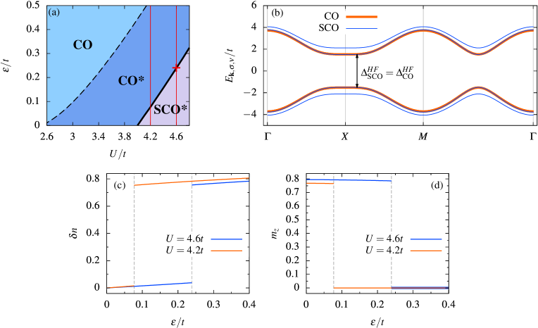
FIG. 1: (a) Zero temperature phase diagram of the half-filled extended Hubbard model in the $(U,\varepsilon)$ plane for $V=t$ within the HF approximation. It comprises a CO region and a SCO region. The phase boundary between the two is denoted by the solid black line. The dashed line corresponds to the SCO end line, along which the SCO solution vanishes. In the CO^∗ (SCO^∗) region the CO and SCO phases coexist with the CO (SCO) one lower in energy. The red cross (lines) indicates the parameters (ranges) used for subsequent plots in this figure. (b) Band structure for the pseudofermions at a SCO-CO transition point. The arrows are indicative of the gaps, which are measured at the $X$ point. Parameters: $U=4.2\leavevmode\nobreak\ t$, $V=t$, and $\varepsilon=0.24\leavevmode\nobreak\ t$. (c) $\delta n$, (d) $m_{\rm z}$ as functions of $\varepsilon$. Parameters: $T=0$, $V=t$, $U=4.2\leavevmode\nobreak\ t$ and $4.6\leavevmode\nobreak\ t$. The gray dashed lines denote transition points.

III Results with the HF approximation

In this section, we investigate the half-filled, zero temperature phase diagram of the above introduced Hubbard model extended by an intersite Coulomb repulsion and a SLP. Results for the half-filled Hubbard model within a similar inhomogeneous crystal field ($\mathcal{H}=\mathcal{H}_{\rm Hub}+\mathcal{H}_{\rm\varepsilon}$) have been obtained in one and two dimensions using Lattice Density Functional Theory Saubanère and Pastor (2009, 2011). On the square lattice, these computations highlighted a continuous phase-transition from the charge-density wave (CDW) phase to a spin-ordered state as the ratio $U/\varepsilon$ is increased. On the other hand, the $t$–$U$–$V$ model ($\mathcal{H}=\mathcal{H}_{\rm Hub}+\mathcal{H}_{\rm V}$) has been thoroughly investigated in the literature. Among the features of this model which attracted great interest is the CDW to spin-density wave (SDW) phase transition at half-filling. The latter has been studied analytically by means of perturbation theory van Dongen (1994a, b) or in the slave boson saddle-point approximation Wolff (1983); Deeg et al. (1993) and numerically from Quantum Monte Carlo (QMC) calculations in one Hirsch (1984); Sengupta et al. (2002) or two Zhang and Callaway (1989) dimensions. More recently, the Dynamical Cluster Approximation (DCA) has been applied to the square lattice Terletska et al. (2017); Paki et al. (2019), yielding a detailed phase diagram of the model at finite temperature in the $U$–$V$ parameter space. To the best of our knowledge, however, no study that simultaneously takes both extensions of the Hubbard model into account has been performed.

The proposed origin of the SLP does not justify the investigation of values of $\varepsilon$ larger than the energy scale $t$. Yet, we show below that small values of $\varepsilon$ may change the nature of the ground state.

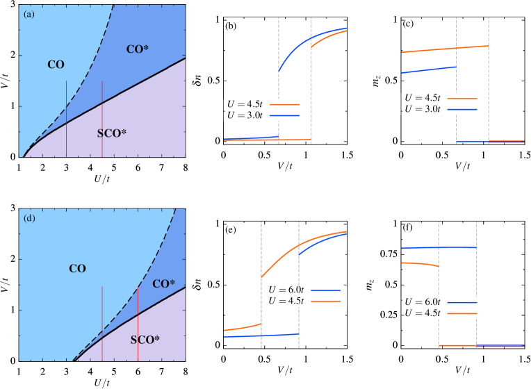
FIG. 2: Zero temperature phase diagram of the half-filled extended Hubbard model in the $(U,V)$ plane for (a) $\varepsilon=0.1\leavevmode\nobreak\ t$, and (d) $\varepsilon=t$ within the HF approximation. It comprises both a CO and a SCO region. The phase boundary between the two is denoted by the solid black line. In the CO^∗ (SCO^∗) region the CO and SCO phases coexist with the CO (SCO) one lower in energy. The end-lines of the two phases are denoted by dashed lines. The red lines indicate the parameters ranges used for subsequent plots in this figure. (b) $\delta n$ and (c) $m_{\rm z}$ as functions of $V$. Parameters: $T=0$, $\varepsilon=0.1\leavevmode\nobreak\ t$, $U=3\leavevmode\nobreak\ t$ and $4.5\leavevmode\nobreak\ t$. (e) $\delta n$ and (f) $m_{\rm z}$ as functions of $V$. Parameters: $T=0$, $\varepsilon=t$, $U=4.5\leavevmode\nobreak\ t$ and $6\leavevmode\nobreak\ t$.

III.1 Influence of the local potential

The zero temperature phase diagram of the three parameter half-filled extended model may be computed through minimization of Eq. (II.2) with respect to $\delta n$, $m_{\rm z}$ and $b_{\rm\sigma}$. Yet, it may be superfluous to scan this three dimensional parameter space and we stick to a series of two dimensional subspaces by attributing a fixed value to the third parameter, aimed at unraveling the most prominent features of the model. We start our investigations maintaining $V$ fixed, and we compute the phase diagram, together with the variations of the order parameters in order to establish the nature of the phase transitions.

The resulting phase diagram is displayed in Fig. 1(a) for fixed $V=t$. It comprises two phases, namely a charge ordered (CO) phase and a spin-and-charge ordered (SCO) phase. The CO* phase corresponds to a region of the phase diagram in which the ground state is CO but SCO-type solutions to the HF self-consistent field equations also exist and usually lie close in energy. The SCO* phase is defined similarly, with SCO being the stable phase. The CO and CO* regions are thus separated by the SCO end-line, which corresponds to the line in parameter space along which SCO solutions vanish and only CO solutions remain. The phase diagram is in line with expectation: while increasing $U$ tends to stabilize the SCO phase, increasing $\varepsilon$ promotes the CO one. For comparatively large $U$ ($U\gtrsim 4\leavevmode\nobreak\ t$), the SCO phase extends down to $\varepsilon=0$, in which case a pure SDW phase is stabilized. This SDW phase entails no charge ordering despite of the finiteness of $V$.

Fig. 1(b) shows the band structure of the two phases at the transition point $U=4.6\leavevmode\nobreak\ t$, $V=t$ and $\varepsilon=0.24\leavevmode\nobreak\ t$. In the CO phase, the band structure is simple, since $\Delta^{\rm HF}_{\rm CO}=(U/2-4V)\delta n-\varepsilon$ for both spin branches. This results in the usual two-band system reminiscent of the CDW phase of the $t$–$U$–$V$ model. In the SCO phase, however, we have $\Delta^{\rm HF}_{\rm SCO,\uparrow}=(U/2-4V)\,\delta n-m_{\rm z}U/2-\varepsilon$ and $\Delta^{\rm HF}_{\rm SCO,\downarrow}=\Delta^{\rm HF}_{\rm SCO,\uparrow}+m_{\rm z}U$. Hence, the spectrum entails four branches, in contrast to the usual two branches of the antiferromagnetic (AFM) phase of the $t$–$U$–$V$ model. Since we work on a half-filled lattice, the four branches are centered around zero and, at zero temperature, the $\nu=-1$ bands are entirely filled while the $\nu=+1$ ones are empty. We also note that the difference in the gaps of the two spin branches, added to the fact that these branches are centered around the same value, yields a symmetry broken phase in which one of the spin branches is higher in energy than the other one. The choice of which branch is higher or lower in energy remains, however, purely arbitrary and is fixed by the sign of $\delta n$ and $m_{\rm z}$ in the SCO solutions. In reality, all four different $(\pm\delta n,\pm m_{\rm z})$ solutions are degenerate and can only be distinguished by their internal parameters. Moreover, since the leading contributions to the Fermi integrals in this regime come from the band minima, we expect the energy of both phases to become nearly degenerate when the minima of the CO $\nu=-1$ band coincide with the highest SCO $\nu=-1$ band. This is precisely what happens at the shown transition point, yielding a SCO-CO phase transition. We can also expect this transition to be discontinuous, as we observe a difference between $\Delta^{\rm HF}_{\rm SCO,\uparrow}$ and $\Delta^{\rm HF}_{\rm SCO,\downarrow}$ of order $2\leavevmode\nobreak\ t/3$, implying that the magnetization in this phase is still large at the transition point and will have to drop down to zero in the CO phase.

In Fig. 1(c) and Fig. 1(d), the $\varepsilon$-dependence of the order parameters at $T=0$, $V=t$ and for fixed values of $U=4.2\leavevmode\nobreak\ t$ and $U=4.6\leavevmode\nobreak\ t$ are shown. We first notice that the charge ordering is more pronounced in the CO phase than it is in the SCO one. Consequently, both phases are still completely distinct at the phase transition, yielding a discontinuous jump of the order parameters characteristic of a first order phase transition. For smaller values of $U$, however, the antiferromagnetic ordering of the spins is somewhat weakened, resulting into slightly less marked discontinuities. Nevertheless, no continuous variation of the order parameters at the transition point has been found in the finite $V$ regime in the relevant $U$ and $\varepsilon$ ranges. The transition is therefore discontinuous.

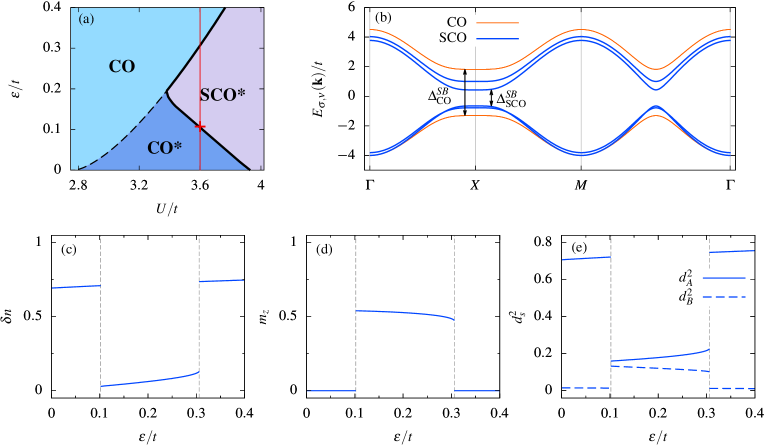
FIG. 3: (a) Zero temperature phase diagram of the half-filled extended Hubbard model in the $(U,\varepsilon)$ plane for $V=t$, within KRSB formalism. It comprises a CO region and a SCO region. The phase boundary between the two is denoted by the solid black line. The dashed line corresponds to the SCO end line, along which the SCO solution to the SPE vanishes. In the CO* (SCO*) region, both solutions exist but the CO (SCO) solution is lower in energy. The red cross (line) indicates the parameters (range) used for subsequent plots in this figure. (b) Band structure for the pseudofermions at a SCO-CO transition point. The arrows are indicative of the gaps, which are measured at the $X$ point. Parameters: $U=3.6\leavevmode\nobreak\ t$, $V=t$, and $\varepsilon=0.1\leavevmode\nobreak\ t$. (c) $\delta n$, (d) $m_{\rm z}$, (e) $d^{\rm 2}_{\rm A}$ and $d^{\rm 2}_{\rm B}$ as functions of $\varepsilon$ for fixed values of $T=0$, $V=t$ and $U=3.6\leavevmode\nobreak\ t$. The gray dashed lines denote transition points.

III.2 Dependence on the screened Coulomb interaction

We now switch to the $U$-$V$ phase diagram. It is presented for $T=0$ and $\varepsilon=0.1\leavevmode\nobreak\ t$ as well as $\varepsilon=t$ in Fig. 2(a) and Fig. 2(d), respectively. Both phases are still separated by a first order transition line but, here, it merges with the SCO end-line at weak couplings. At stronger couplings, the transition line at fixed $\varepsilon$ becomes linear in $U$: $V(U)\simeq U/4$ for $U,V\gg\varepsilon$. This $V(U)\propto U/4$ dependence is evocative of the already reported $V=U/4$ CDW-SDW transition line of the half-filled $t$–$U$–$V$ model (see Refs. [van Dongen, 1994a, b; Wolff, 1983; Deeg et al., 1993; Hirsch, 1984; Sengupta et al., 2002; Zhang and Callaway, 1989; Terletska et al., 2017; Paki et al., 2019]) that we address below. This is to be expected as, in a coupling regime in which $\varepsilon$ becomes negligible, one should recover results qualitatively similar to those of the $t$–$U$–$V$ model (in which $\varepsilon=0$). This also explains why the beginning of this linear regime is shifted towards stronger couplings as $\varepsilon$ is increased from $0.1\leavevmode\nobreak\ t$ [Fig. 2(a)] to $t$ [Fig. 2(d)].

In Fig. 2(b) and Fig. 2(c) the zero temperature variations of the order parameters are presented, for representative parameter sets, as functions of V. We set $\varepsilon=0.1\leavevmode\nobreak\ t$, together with $U=3\leavevmode\nobreak\ t$ and $U=4.5\leavevmode\nobreak\ t$. In Fig. 2(e) and Fig. 2(f) the same variations are presented but for fixed $\varepsilon=t$, and for values of $U=4.5\leavevmode\nobreak\ t$ and $U=6\leavevmode\nobreak\ t$. We obtain a single SCO-CO transition for each parameters set, for $V=0.67\leavevmode\nobreak\ t$, $1.14\leavevmode\nobreak\ t$, $0.46\leavevmode\nobreak\ t$ and $0.91\leavevmode\nobreak\ t$, respectively. The order parameters again vary discontinuously at these transitions. We also note that this discontinuity is preserved at weaker and stronger couplings. We see, however, that the discontinuity is softened for larger values of $\varepsilon$ and/or smaller values of $U$. This owes to the stronger antiferromagnetic ordering of the spins and weaker charge ordering at large values of $U/\varepsilon$, yielding a sharper drop (increase) in $m_{\rm z}$ ($\delta n$) at the SCO to CO transition. Combining these results with the ones of the previous section, we conclude that, in the HF approximation, the SCO-CO phase transition occurring at zero temperature, and half-filling, is discontinuous. In addition, the phase diagram exhibits a phase boundary between the CO* and SCO* in a large range of couplings, which may be suitable for resistive switching.

IV Results with the KRSB representation

As highlighted in, e.g., Ref. [Steffen et al., 2017], the HF approximation and the KRSB representation of extended (or not) Hubbard models are in good quantitative agreement in the weak-coupling regime. However, one can hardly expect the HF approximation to yield quantitatively appreciable results in the intermediate-to-strong coupling regime due to the inherent inability of such mean field techniques to account for strong correlations. On the other hand, as outlined earlier, slave boson techniques have proved their efficiency in the stronger coupling regimes Frésard et al. (2012, 1991, 2022); Riegler et al. (2020); Igoshev et al. (2015); Timirgazin et al. (2016); Igoshev and Irkhin (2021). The KRSB representation thus appears as a convenient tool to assess for the relevance of the correlations in the strong coupling regime of the model and we shall use it to that aim in this section.

IV.1 Influence of the local potential

Let us now show the results following from the solution of the saddle-point equations Eq. (56) and discuss them in the next two paragraphs. Emphasized is the competition between the different orders in the phase diagram. An identification of the lowest energy solution — with the free energy per lattice site $F=\Omega/N_{\rm L}+\mu$ — allows us to determine the stable phase for given values of the parameters and we study the variations of the order parameters $\delta n$, $m_{\rm z}$ and $d^{\rm 2}_{\rm s}=\langle n_{\rm i,\uparrow}n_{\rm i,\downarrow}\rangle|_{\rm i\in s}$ in order to confirm the nature of the different phase transitions.

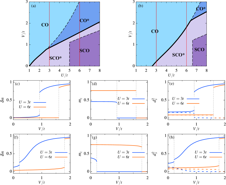
FIG. 4: Zero temperature phase diagram of the half-filled extended Hubbard model in the $(U,V)$ plane for (a) $\varepsilon=0.1\leavevmode\nobreak\ t$, and (b) $\varepsilon=t$, within KRSB formalism. It comprises both a CO and a SCO region. The phase boundary between the two is denoted by the solid black line. In the CO^∗ (SCO^∗) region the CO and SCO phases coexist with the CO (SCO) one lower in energy. The end-lines of the two phases are denoted by dashed lines. The red lines indicate the parameter ranges used for subsequent plots in this figure. (c) $\delta n$, (d) $m_{\rm z}$, (e) $d^{\rm 2}_{\rm A}$ and $d^{\rm 2}_{\rm B}$ as functions of $V$. Parameters: $T=0$, $U=3\leavevmode\nobreak\ t$ and $\varepsilon=0.1\leavevmode\nobreak\ t$. (f) $\delta n$, (g) $m_{\rm z}$, (h) $d^{\rm 2}_{\rm A}$ (solid line) and $d^{\rm 2}_{\rm B}$ (dashed line) as functions of $V$. Parameters: $T=0$, $\varepsilon=t$, $U=3\leavevmode\nobreak\ t$ and $6\leavevmode\nobreak\ t$.

The resulting phase diagram is displayed in Fig. 3(a) as a function of $U$ and $\varepsilon$ at zero temperature and fixed $V=t$. It comprises a CO and a SCO region, separated by a phase boundary across which a first order phase transition occurs. The lowermost ($\varepsilon\lesssim 0.2\leavevmode\nobreak\ t$) segment of this transition line corresponds to the $F_{\rm CO}=F_{\rm SCO}$ degeneracy line while the uppermost ($\varepsilon\gtrsim 0.2\leavevmode\nobreak\ t$) segment lies along the SCO end-line. This is in contrast to the HF phase diagram in $U$-$\varepsilon$ space, in which the phase boundary only consists of the CO-SCO degeneracy line. Above the SCO end-line, the CO phase is stabilized by default, irrespective of its energy. Below this line, for lower couplings ($U\lesssim 3.8\leavevmode\nobreak\ t$), we find a dome in the CO phase in which the SCO solution still exists and lies close in energy. The SCO phase is thus meta-stable under this dome, implying coexistence of both phases in this regime. In addition, a pure SDW phase is stabilized for $\varepsilon=0$ and $U\gtrsim 3.5\leavevmode\nobreak\ t$ as already encountered in the HF phase diagram Fig. 1(a).

Fig. 3(b) presents the band structure of the two phases at a given transition point $U=3.6\leavevmode\nobreak\ t$, $V=t$ and $\varepsilon=0.102\leavevmode\nobreak\ t$. In the CO phase, $\tilde{\mu}_{\rm\uparrow}=\tilde{\mu}_{\rm\downarrow}$ (with $\tilde{\mu}_{\rm\sigma}=\mu-\overline{\beta}_{\rm\sigma}$) and $\Delta^{\rm SB}_{\rm\uparrow}=\Delta^{\rm SB}_{\rm\downarrow}$, resulting into the two spin branches being equivalent. Besides, no such simplification holds in the SCO phase, leading to four distinct bands. Analogously to what has been discussed in Sec. III, the SCO solution has a broken spin-rotation symmetry, with two inequivalent spin branches. As in the HF approximation, the lowest and highest energy branches are fixed by the sign of $\delta n$ and $m_{\rm z}$, while the four different $(\pm\delta n,\pm m_{\rm z})$ solutions remain degenerate. Since we are at half-filling, the Lagrange multipliers and the chemical potential satisfy $|\tilde{\mu}_{\rm\sigma}|<|\Delta^{\rm SB}_{\rm\sigma}|/2$, such that only the $\nu=-1$ bands are filled, while the $\nu=+1$ bands remain empty. Looking at these lower bands, we see that — at this transition point in $U$-$V$-$\varepsilon$ space — the minima of the bands in the SCO phase overlaps with its counterpart in the CO phase. Varying the parameters towards the CO (SCO) stability region of the phase diagram results in the lowering of the minima of the CO (SCO) lower band. Since we are at zero temperature, the contributions to the Fermi integrals largely follows from these lower bands minima. The stable phase for a given set of parameters can thus be suggested by inspection of the latter. Besides, $\Delta^{\rm SB}_{\rm CO}$ markedly differs from $\Delta^{\rm SB}_{\rm SCO}$ even though both phases are degenerate in energy. Hence, the value of the gap may not be used to predict the nature of the ground state.

The variation of the order parameters is given in Fig. 3(c), Fig. 3(d), and Fig. 3(e) as a function of $\varepsilon$ and for fixed values of $T=0$, $U=3.6\leavevmode\nobreak\ t$ and $V=t$. We notice that the local charge and pair modulations are substantially larger in the CO phase than in the SCO one. For these parameters, two consecutive transitions between the two phases occur as $\varepsilon$ is increased ($\varepsilon\approx 0.1\leavevmode\nobreak\ t$ and $\varepsilon\approx 0.3\leavevmode\nobreak\ t$). We see that, at the transition points, all order parameters vary discontinuously. This implies the CO-SCO transition to be first order. At finite $V$, no region of parameter space has been found to exhibit a continuous variation of the order parameters across the phase boundary. However, the discontinuity in the variation of the order parameters at the transition points become less important as $\varepsilon$ and $V$ increase or as $U$ decreases. As detailed in the next paragraph, the SCO phase is restricted to small values of $V/U$, while large values of $\varepsilon/U$ are irrelevant due to the proposed origins for the $\varepsilon$-term. This shows that no continuous CO-SCO transition is possible in the parameter range of interest.

IV.2 Dependence on the screened Coulomb interaction

Turning now to the explicit dependence on $V$ of the phase diagram, we present in Fig. 4(a) and Fig. 4(b) the zero-temperature phase diagram of the model as a function of $U$ and $V$, for $\varepsilon=0.1\leavevmode\nobreak\ t$ and $\varepsilon=t$. At weak couplings, the CO-SCO phase boundary merges with the SCO end-line [uppermost segment of the phase boundary in Fig. 4(a)]. At stronger couplings, however, the transition line between the two phases digresses from the SCO end-line and a $F_{\rm CO}=F_{\rm SCO}$ degeneracy line begins [lowermost part of the phase boundary in Fig. 4(a)]. In this regime, the transition line gradually becomes linear, such that it can ultimately be parametrized by $V=U/4+c(\varepsilon)$ for $U,V\gg\varepsilon$, with $c(\varepsilon)$ independent of $U$ and $V$. We computed $c(\varepsilon=0.1\leavevmode\nobreak\ t)\approx 0.06\leavevmode\nobreak\ t$ and $c(\varepsilon=t)\approx 0.53\leavevmode\nobreak\ t$ for these two phase diagrams. This strong coupling behavior is in qualitative disagreement with the one observed in the HF approximation. Indeed, the staggered potential appears to favor the stabilization of the SCO phase at large $U$ while, in the HF approximation, the SCO-CO transition line lies slightly below the $V=U/4$ line at strong coupling — evidencing the role of correlations in the mechanisms underlying this phase transition in the strong coupling regime. Let us also notice the vertical part of the CO end-line at $U=5\leavevmode\nobreak\ t$ and $6.2\leavevmode\nobreak\ t$ for $\varepsilon=0.1\leavevmode\nobreak\ t$ and $t$, respectively. This follows from the fact that, for $U$ larger than these values, the charge order is generated by $\varepsilon$ alone and values of $V$ smaller than $t$ and $1.2\leavevmode\nobreak\ t$, respectively, do not yield additional charge order in the CO phase. In the $\varepsilon=0$ case, as discussed below, this would result in a disordered paramagnetic phase, which is prohibited here due to the minimal charge ordering imposed by $\varepsilon$.

The zero temperature variations of the order parameters as a function of $V$, for fixed $U=3\leavevmode\nobreak\ t$ and $U=6\leavevmode\nobreak\ t$ are shown in Fig. 4(c), Fig. 4(d) and Fig. 4(e) for $\varepsilon=0.1\leavevmode\nobreak\ t$, and in Fig. 4(f), Fig. 4(g) and Fig. 4(h) for $\varepsilon=t$. Along these paths in parameter space, there is a single CO-SCO transition at $V\approx 0.9\leavevmode\nobreak\ t$ for $\varepsilon=0.1\leavevmode\nobreak\ t$ and at $V\approx 0.2\leavevmode\nobreak\ t$ for $\varepsilon=t$. The order parameters vary discontinuously at this transition. Such jumps of order parameters happen as well in the linear regime of the transition line. We see that, for smaller values of $\varepsilon$, the discontinuity is enhanced. We also observe such an enhancement when $U$ is increased. This is explained by the fact that the SCO configurations become increasingly antiferromagnetically ordered and decreasingly charge ordered, and conversely for smaller values of $U$ and larger values of $\varepsilon$. Additionally, we note that small values of $\varepsilon$ with respect to the energy scales of $U$ and $V$ ($\varepsilon=0.1\leavevmode\nobreak\ t$ compared to $U\geq t$ and $V\sim t$) are sufficient to establish strongly discontinuous transitions. For reasons outlined above, values of $\varepsilon$ larger than the energy scale $t$ have not been investigated. Moreover, in the small $U$ regime, the SCO phase is not stabilized, even for arbitrarily small values of $V$ if $\varepsilon$ is of the order of $t$. As a consequence to this, no transition point has been found to correspond to a continuous transition at finite $\varepsilon$. In addition to the statement that no second order transition occurs in $U$–$\varepsilon$ space for finite $V$, this leads to the conclusion that the CO-SCO transition at zero temperature is systematically of first order. Furthermore, phase coexistence, suitable for resistive switching, has been established in a large domain of the phase diagram.

The way the SCO solution ceases to exist is reminiscent of the $U_{\rm c1}$ and $U_{\rm c2}$ lines of the two-band model in its $U$-dependence as described in the suitably extended KR representation. There, for densities sufficiently close the half-filling and finite $J_{\rm H}$, the quasiparticle residue acquires a vertical tangent and so does the free energy Frésard and Lamboley (2002); Frésard et al. (2022). In other words, these singular points mark the end point of the insulating, resp. metallic solutions. In the current case, the staggered magnetization of the SCO phase acquires a vertical tangent in its $V$-dependence (see Fig. 4), too, which is reflected in the $V$-dependence of the free energy as well. Hence, this singular point denotes the end point of the SCO phase which, depending on the parameter values, may correspond to the phase transition. For instance, this is the case for $t\lesssim U\lesssim 2.8\leavevmode\nobreak\ t$ with $\varepsilon=0.1\leavevmode\nobreak\ t$, while for $\varepsilon=t$, this happens for $2.5\leavevmode\nobreak\ t\lesssim U\lesssim 6.5\leavevmode\nobreak\ t$. For larger $U$-values, the phase transition does not correspond to the end point of the SCO phase any longer.

IV.3 Resistive switching

Let us here briefly consider temperature driven SCO-CO phase transitions. They take place at temperatures scaling with the gap between the empty and occupied quasi-particle bands, which itself scales with $U$ when it is the largest energy into play. In that case, the largeness of the gap implies that the band filling is mostly independent of $T$ at small temperatures, leading to a high transition temperature. Yet, the situation changes in the intermediate coupling regime. For instance, we performed calculations with $U=4.2\leavevmode\nobreak\ t$, $V=t$ and $\varepsilon=0.1\leavevmode\nobreak\ t$, i. e. in the SCO phase close to its boundary, and we obtained the temperature at which the magnetic order melts to be close to 0.35 t while the SCO-CO transition was obtained at a lower $T_{\rm SCO-CO}\simeq 0.2\leavevmode\nobreak\ t$. Recalling that the hopping amplitude in transition metal oxides is widely accepted to be in the $0.1$ eV to $0.3$ eV range, it renders $T_{\rm SCO-CO}$ experimentally accessible.

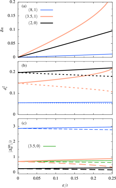
FIG. 5: (a) $\delta n$, (b) $d^{\rm 2}_{\rm A}$ (solid line) and $d^{\rm 2}_{\rm B}$ (dashed line), (c) $|\Delta^{\rm SB}_{\rm\uparrow}|$ (solid line) and $|\Delta^{\rm SB}_{\rm\downarrow}|$ (dashed line) in the SCO phase as functions of $\varepsilon$ for different values of the couple $(U,V)$. These order parameters have been computed within KRSB formalism. Parameters: $T=0$, $(U/t,V/t)=(8,1)$ (blue), $(3.5,1)$ (orange), $(2,0)$ (black) and $(3.5,0)$ (green) in the last panel.

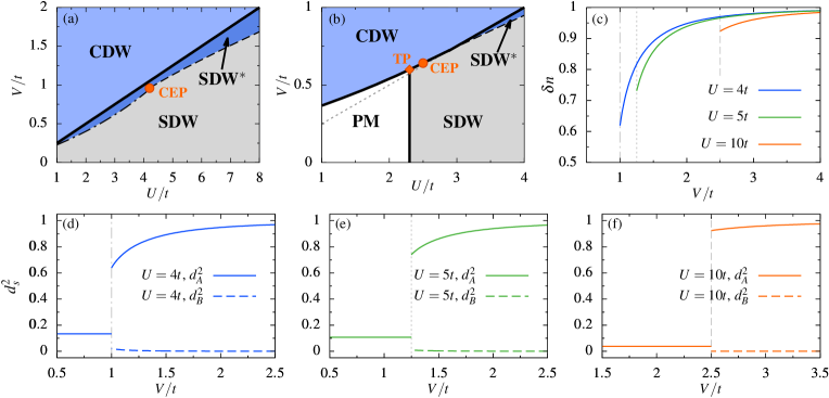
FIG. 6: KRSB phase diagram of the half-filled $t$–$U$–$V$ model at (a) zero temperature and (b) $T=t/6$ in the $(U,V)$ plane. The phase boundaries are denoted by solid black lines. The dashed lines correspond to the CDW end-line, while the dash-dotted line denotes the PM-CDW instability line. The PM-CDW-SDW triple point (TP) is denoted by an orange diamond. The PM-CDW instability critical end-point (CEP) is denoted by an orange circle. In the SCO^∗ region the CDW and SCO phases coexist, with the latter one being lower in energy. (c) $\delta n$ as a function of $V$ at $T=0$ for $U=4\leavevmode\nobreak\ t$, $U=5\leavevmode\nobreak\ t$ and $U=10\leavevmode\nobreak\ t$. (d), (e) and (f) show $d^{\rm 2}_{\rm A}$ and $d^{\rm 2}_{\rm B}$ as a function of $V$ at $T=0$ and for $U=4\leavevmode\nobreak\ t$, $U=5\leavevmode\nobreak\ t$ and $U=10\leavevmode\nobreak\ t$, respectively. The gray lines correspond to the SDW-CDW transition points for the different values of $U$.

V The t–U–V limit

V.1 Zero temperature results

As outlined in Sec. IV, the SCO phase is not observed in the $\varepsilon=0$ limit. The reason is that the SCO solution continuously becomes a pure SDW phase as $\varepsilon\to 0$. As can be seen from Fig. 5(a), in this limit, we find that in the SCO solutions, $\delta n$ goes to zero for all values of $U$ and $V$. A similar effect is also shown to occur for the double occupancies in Fig. 5(b), in which $d^{\rm 2}_{\rm A}$ and $d^{\rm 2}_{\rm B}$ merge to a unique value at $\varepsilon=0$. On the other hand, the staggered magnetization $m_{\rm z}$ remains finite, leading to a SDW phase with no charge order. As for the values of the SCO band-gaps, which are displayed in Fig. 5(c), they similarly merge towards a unique value upon reduction of $\varepsilon$ as evidenced by the $(U/t,V/t)=(3.5,0)$ and $(3.5,1)$ plots. Moreover, the value of this single gap at $\varepsilon=0$ remains $V$-independent, which hints at the independence in $V$ of the charge-homogeneous solutions to the SPE discussed below.

In this limit, the model reduces to the $t$–$U$–$V$ model. Its zero temperature phase diagram is displayed in Fig. 6(a) in dependence on $U$ and $V$. It features two phases, namely the SDW and the CDW phases. They are separated by the aforementioned $V=U/4$ phase boundary, across which a first order transition occurs. Below this phase boundary, the CDW solutions continue to exist in a finite region delimited by the PM-CDW instability line (along which $\delta n=0$ and $F_{\rm PM}=F_{\rm CDW}$) and the CDW end line (as defined in previous sections). These two lines meet at the critical end point (CEP) where the PM-CDW instability vanishes. Beyond this point, no CDW solutions with arbitrarily small values of $\delta n$ are found.

Fig. 6(c), Fig. 6(d), Fig. 6(e) and Fig. 6(f) provide an overview of the variations of $\delta n$ and $d^{\rm 2}$ in the CDW phase as functions of $V$ for representative values of $U$: $U=4\leavevmode\nobreak\ t$, $5\leavevmode\nobreak\ t$ and $10\leavevmode\nobreak\ t$, at zero temperature. For these values, the CDW-SDW transition occurs at $V=t$, $V=1.25\leavevmode\nobreak\ t$ and $V=2.5\leavevmode\nobreak\ t$, respectively. Let us notice that, for large $U$ ($U>10\leavevmode\nobreak\ t$), the CDW phase closely resembles a pair density wave (PDW), as the double occupancy oscillates between nearly zero and nearly one while the single occupancy is strongly suppressed. Furthermore, this PDW shows little dependence on $V$ when the latter is larger than $U/4$. Upon reducing $U$, the PDW gradually turns into a genuine CDW. In all cases, we see that the order parameters discontinuously jump across the transition. More generally, no value of $U$ has been found to exhibit a continuous CDW-SDW transition. Instead, $\delta n$ systematically discontinuously goes from a finite value to zero at the CDW-SDW transition point, assessing the phase transition to be of first order.

V.2 Finite temperature results

In Fig. 6(b), the phase diagram of the model is shown for $T=t/6$ as a function of $U$ and $V$. It exhibits an additional phase at weak couplings, namely the PM phase. As explained below, the PM-CDW and PM-SDW phase boundaries follow from second order phase transitions. The SDW-CDW transition however remains of first order. Similarly to the $T=0$ case, the transition line in the strong coupling regime corresponds to the $V=U/4$ line. This result agrees with QMC simulations Zhang and Callaway (1989) and DCA calculations Terletska et al. (2017); Paki et al. (2019).

In addition, we compared the free energy of the SDW phase at $U=1.9\leavevmode\nobreak\ t$ and $V=0.4\leavevmode\nobreak\ t$ and $\beta=100\leavevmode\nobreak\ t/3$ with the determinantal QMC (DQMC) results given in the supplemental material of Ref. [Sushchyev and Wessel, 2022]. They found an energy of $-0.453t$, whereas we find an energy of $-0.299\leavevmode\nobreak\ t$ in the HF approximation and $-0.387\leavevmode\nobreak\ t$ in the KRSB formalism. Hence, the energy difference between the DQMC and KRSB energies is as small as $8\times 10^{\rm-2}\leavevmode\nobreak\ W$, with $W$ the bare bandwidth. This supports prior agreement between both approaches. Note that, in the context of the t-U Hubbard model, the energy difference between QMC and KRSB is largest for U around 2t (see Ref. [Lilly et al., 1990]).

Moreover, the parameter region for the PM phase is in rather good quantitative agreement with DCA results. We also observed that the PM-CDW transition line deviates from the $V=U/4$ line at weak couplings, while a region of CDW-SDW coexistence develops at strong couplings. Our PM-SDW phase boundary does not, however, depend on $V$ while DCA predictions point towards a weak $V$-dependence. We identify two points of particular relevance: the CEP, as defined for Fig. 6(a) and a triple point (TP) where the PM, CDW and SDW solutions become degenerate. Most notably, when compared to Fig. 6(b), the CEP is shifted towards weaker couplings.

The only regime in which we can define a continuous transition between the CDW phase and the SDW phase is at finite temperature. Since the PM region in Fig. 6(b) is bounded by the PM-SDW and PM-CDW instability lines, we can take a path in $U$–$V$ space starting from, e. g., the CDW region, going through the PM region and finally ending in the SDW region. This would yield a path along which only continuous variations of the order parameters are observed, with $\delta n$ going from a finite value in the CDW region down to zero in the PM region and $m_{\rm z}$ going from zero in the PM region to a finite value in the SDW region.

It is important to note that, despite close investigation in the region around the SDW-CDW transition line and the $F_{\rm PM}=F_{\rm CDW}=F_{\rm SDW}$ triple point, no joint spin-and-charge modulated solution to the SPE could be obtained. This, and the collapse of the SCO order in the whole $U$–$V$ range in the $\varepsilon\to 0$ limit, hints that breaking the $n_{\rm A}=n_{\rm B}=1$ symmetry of the SDW phase in the half-filled $t$–$U$–$V$ model might yield, if any, an order more intricate than the SCO one.

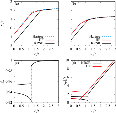
FIG. 7: Zero temperature free energy obtained from the Hartree (dotted blue), HF (solid red), and KRSB (solid black) calculations as functions of $V$. (c) Slave-boson renormalization factors and (d) Slave-boson (black) and HF (red) gaps as functions of $V$. The dotted lines denote discontinuous jumps at the phase transition. Parameters: (a) $U=5\leavevmode\nobreak\ t$, $\varepsilon=t/10$, (b), (c) and (d) $U=5\leavevmode\nobreak\ t$, $\varepsilon=t$.

VI Effect of correlations

In this section, we assess for the relevance of correlations by comparing the phase diagrams as well as the free energies obtained in the HF approximation and in the KRSB formalism. We also focus on possible markers of a strongly-correlated phase, namely the slave-boson renormalization factors as well as the difference between the gaps in the dispersion obtained in each method.

Qualitatively our HF and KRSB calculations support a series of common conclusions. The phase diagrams are both made of CO and SCO regimes and entail large phase coexistence regions. Yet, they markedly differ from the quantitative point of view. For instance, for $V=t$, the SCO phase may be found for $U$ as small as $3.4\leavevmode\nobreak\ t$ in KRSB formalism, while it takes $U=4\leavevmode\nobreak\ t$ to stabilize it in the HF approximation. In addition, their $(U,\varepsilon)$ phase diagram differ in the shape of their phase boundaries. Specifically, by continuously increasing $\varepsilon$ at fixed $U>3.4\leavevmode\nobreak\ t$, a transition from the CO phase to the SCO phase is found, while a second transition back to the CO phase arises in the KRSB phase diagram. This re-entrant behavior is absent in the HF phase diagram in $(U,\varepsilon)$ space where only a single phase transition is possible when increasing $\varepsilon$.

These discrepancies between the phase diagrams obtained by both methods follow from the difference between the free energy obtained in the HF approximation and the one obtained in the KRSB representation. Fig. 7(a) and Fig. 7(b) present the zero temperature free energies obtained in the Hartree approximation, HF approximation and in the KRSB formalism as functions of $V$ for $U=5\leavevmode\nobreak\ t$ and $\varepsilon=t/10$ as well as $\varepsilon=t$, respectively. At small values of $V$, the stable phase is the SCO one. In this phase, the leading energy scale is that of $U$. This leads to the HF energy being approximately $80\%$ ($58\%$) higher than the KRSB energy for $\varepsilon=t/10$ ($t$), due to the non-negligible $U$-induced correlation in this phase. At larger values of $V$, however, the CO phase is stabilized. In this regime, the dominating coupling scale becomes $V$ and the HF and KRSB energies differ by less than $0.1\%$. The HF energy is actually slightly lower than its KRSB counterpart. This minor difference can be explained by the increasing relevance of the exchange term Eq. (16) for larger values of $V$, while no such contribution of the exchange to the energy arises in the KRSB formalism.

The slave-boson renormalization factors are displayed in Fig. 7(c) as functions of $V$, for $U=5\leavevmode\nobreak\ t$ and $\varepsilon=t$. In the large $V$ regime, we see that $\tilde{z}$ quickly goes to one, in which case the effective dispersions Eq. (15) and Eq. (31) seem to closely resemble one another. Yet, the differences between the two are sizable as the gap of the HF dispersion is larger than its KRSB counterpart. As for the SCO phase, we see that, albeit close to one, $\tilde{z}_{\rm\uparrow}$ and $\tilde{z}_{\rm\downarrow}$ do not reach one. This portrays a slightly correlated phase, the energy of which must then differ from the HF energy, as evidenced in the previous paragraph.

In Fig. 7(d), the band gaps obtained in the HF approximation and in the KRSB representation are displayed as functions of $V$, for $U=5\leavevmode\nobreak\ t$ and $\varepsilon=t$. We notice that the HF gaps also markedly differ from the KRSB gaps, especially in the SCO phase where the largest $|\Delta_{\rm\sigma}|$ in the HF approximation is approximately $50\%$ larger than its KRSB counterpart. This may also lead to free energy discrepancies between both methods.

VII Conclusion and outlook

Summarizing, we have set up and addressed a microscopical $t$–$U$–$V$–$\varepsilon$ model supporting a spin-and-charge ordered phase in its phase diagram in two dimensions at half-filling. Such a phase is intuitively expected to smoothly connect the spin density wave ground state of the half-filled Hubbard model and the charge density wave of the half-filled $t$–$U$–$V$ extended Hubbard model. Our findings do not support this expectation and, at zero temperature, we unraveled discontinuous transitions only, apart from the celebrated instability to Néel order for $U=V=\varepsilon=0$. Furthermore, the SCO order systematically collapses when $\varepsilon$ is suppressed down to zero, irrespective of the values of $U$ and $V$. The splitting is therefore essential to the stabilization of the SCO phase.

Let us emphasize that the staggered local potential is also pivotal to the first order phase transition that we could relate to resistive switching. As compared to the intensely sought for superconductivity, its associated temperature is larger by about one order of magnitude, or even more, making it easier to observe. Beyond materials, cold atoms offer a possibility to experimentally unravel this transition, too, as they can easily be submitted to the SLP and since the transition temperature may be of order $t$.

For fixed, moderate $V$, our HF phase diagram of the $t$–$U$–$V$–$\varepsilon$ model at half-filling comprises both the CO and SCO phases. In the $U$-$\varepsilon$ plane, the phase transition is discontinuous and the phase boundary is well approximated by a simple straight line $\varepsilon_{\rm crit}\propto U$ that is located within a CO and SCO coexistence region. In contrast, in the KRSB formalism, the SCO phase displays a re-entrant behavior: starting from a critical point ($\varepsilon\simeq 0.2\leavevmode\nobreak\ t$, $U\simeq 3.4\leavevmode\nobreak\ t$), two phase boundary lines develop. A first one where $\varepsilon_{\rm crit}$ increases about linearly with $U$, and a second one where $\varepsilon_{\rm crit}$ decreases about linearly with $U$. In the former case, the phase boundary corresponds to the end line of the SCO phase, while in the latter case we obtain a discontinuous transition inside a CO and SCO coexistence region. This robustness of the SCO phase in KRSB formalism is rooted in its ability to jointly take magnetism and effective mass renormalization into account, which leads to a sizable lowering of the free energy.

There is a lesser degree of divergence when it comes to the comparison of the HF and KRSB phase diagrams for fixed $\varepsilon$ from the qualitative point of view. Yet, in KRSB, the phase boundary between the SCO and CO phases is made of two pieces for both small and large $\varepsilon$-values. The first segment, for small $V$-values, corresponds to the end points of the SCO phase, while for large $V$-values, it corresponds to the free energy crossing of the CO and SCO solutions, in a regime where both phases coexist. This transition is discontinuous. In contrast, the HF approach yields this phase boundary to be made of the second piece only, at the exception of a small $\varepsilon$-small $V$ regime ($V\lesssim 0.2\leavevmode\nobreak\ t$). Moreover, no pure SCO phase is predicted at the HF level, while the KRSB approach predicts that only the SCO phase is stabilized in the large $U$-smaller $V$ regime ($V<U/4$), irrespective of the value of $\varepsilon$. That the end line of the CO phase is missed in HF may not be very astonishing, as it happens for rather large $U$-values, where HF theory is not controlled.

Regarding the pure $t$–$U$–$V$ model at finite temperature, the ground states are not systematically ordered any longer, especially in the weak coupling regime. Accordingly, instability lines towards SDW and CDW phases are found and it becomes possible to go continuously from the former to the latter. There is obvious interest to the unraveling of the influence of doping on the phase diagram, and work towards this end is in progress.

Appendix A Hartree-Fock self-consistent field equations

Minimizing Eq. (II.2) with respect to the different order-parameters yields the following equations,

$$1=\sum_{\rm\sigma}\mathcal{J}_{\rm 0,\sigma},$$ (36a)

$$\delta n=\sum_{\rm\sigma}\mathcal{J}_{\rm 1,\sigma},$$ (36b)

$$m_{\rm z}=\sum_{\rm\sigma}\underline{\tau}^{\rm 3}_{\rm\sigma\sigma}\mathcal{J}_{\rm 1,\sigma},$$ (36c)

$$b_{\rm\uparrow}=\mathcal{K}_{\rm\uparrow},$$ (36d)

$$b_{\rm\downarrow}=\mathcal{K}_{\rm\downarrow},$$ (36e)

$$\delta b_{\rm\uparrow}=\delta b_{\rm\downarrow}=0,$$ (36f)

with

$$\mathcal{J}_{\rm m,\sigma}=\frac{1}{N_{\rm L}}\sum_{\textbf{k},\nu}{\vphantom{\sum}}^{\prime}n_{\rm F}(E_{\rm\textbf{k},\sigma,\nu})\left[\frac{\nu\Delta^{\rm HF}_{\rm\sigma}}{\sqrt{(t^{\rm eff}_{\rm\textbf{k},\sigma})^{\rm 2}+(\Delta^{\rm HF}_{\rm\sigma})^{\rm 2}}}\right]^{\rm m},$$ (37a)

$$\mathcal{K}_{\rm\sigma}=\frac{1}{N_{\rm L}}\sum_{\textbf{k},\nu}{\vphantom{\sum}}^{\prime}n_{\rm F}(E_{\rm\textbf{k},\sigma,\nu})\frac{\nu t^{\rm eff}_{\rm\textbf{k},\sigma}(\cos k_{\rm x}+\cos k_{\rm y})}{4\sqrt{(t^{\rm eff}_{\rm\textbf{k},\sigma})^{\rm 2}+(\Delta^{\rm HF}_{\rm\sigma})^{\rm 2}}},$$ (37b)

and where $n_{\rm F}(E_{\rm\textbf{k},\sigma,\nu})$ is the Fermi function

$$n_{\rm F}(E_{\rm\textbf{k},\sigma,\nu})=\frac{1}{1+\exp(\beta E_{\rm\textbf{k},\sigma,\nu})}.$$ (38)

Appendix B Treatment of the slave boson saddle-points

B.1 Expression of the KRSB grand potential

We study the saddle-point configurations of the grand potential by imposing symmetries on the saddle-point solutions in order to describe the phases that we found to be of relevance. They are the paramagnetic (PM), charge ordered (CO), spin density wave (SDW), or spin-and-charge order (SCO) phases. None of them carry net magnetization. This is taken care of by the following relationship between the bosons:

$$m^{\rm\phantom{X}}_{\rm z,A}+m^{\rm\phantom{X}}_{\rm z,B}=p^{\rm 2}_{\rm A,\uparrow}-p^{\rm 2}_{\rm A,\downarrow}+p^{\rm 2}_{\rm B,\uparrow}-p^{\rm 2}_{\rm B,\downarrow}=0.$$ (39)

It may be satisfied by the relations

$$p^{\rm 2}_{\rm A,\uparrow}=p^{\rm 2}_{\rm B,\uparrow},$$ (40a)

$$p^{\rm 2}_{\rm A,\downarrow}=p^{\rm 2}_{\rm B,\downarrow},$$ (40b)

but this is not the only solution. In fact, the lowest in energy solution generally does not fulfill Eq. (40). Besides, the half filled lattice condition is translated as:

$$n_{\rm A,\sigma}+n_{\rm B,\sigma}=p^{\rm 2}_{\rm A,\sigma}+d^{\rm 2}_{\rm A}+p^{\rm 2}_{\rm B,\sigma}+d^{\rm 2}_{\rm B}=1.$$ (41)

No further symmetry is imposed on an SCO configuration, that corresponds to the lowest symmetry phase. All seven unknown saddle-point parameters for each sublattice may thus be gathered as

$$\psi^{\rm SCO}_{\rm s}=\left(e^{\vphantom{\dagger}}_{\rm s},d^{\vphantom{\dagger}}_{\rm s},0,p^{{\vphantom{\dagger}}}_{\rm s,\uparrow},p^{{\vphantom{\dagger}}}_{\rm s,\downarrow},\beta^{{\vphantom{\dagger}}}_{\rm s,\uparrow},\beta^{{\vphantom{\dagger}}}_{\rm s,\downarrow},\alpha^{{\vphantom{\dagger}}}_{\rm s}\right).$$ (42)

In order to generate a CO configuration, we add another condition, namely that the magnetization vanishes on each sublattice. It reads

$$m^{\rm\phantom{X}}_{\rm z,s}=p^{\rm 2}_{\rm s,\uparrow}-p^{\rm 2}_{\rm s,\downarrow}=0,$$ (43)

This yields a charge-ordered nonmagnetic saddle point for which the five unknowns for each sublattice may be gathered as

$$\psi^{\rm CO}_{\rm s}=\left(e_{\rm s},d_{\rm s},0,p^{{\vphantom{\dagger}}}_{\rm s},p^{{\vphantom{\dagger}}}_{\rm s},\beta^{{\vphantom{\dagger}}}_{\rm s},\beta^{{\vphantom{\dagger}}}_{\rm s},\alpha^{{\vphantom{\dagger}}}_{\rm s}\right),$$ (44)

In the SDW phase, the local magnetization is finite but takes opposite values on each sublattice, so that

$$m^{\rm\phantom{X}}_{\rm z,A}=-m^{\rm\phantom{X}}_{\rm z,B}\neq 0.$$ (45a)

Moreover, the density is fixed to one on each sublattice

$$n_{\rm s}=p^{\rm 2}_{\rm s,\uparrow}+p^{\rm 2}_{\rm s,\downarrow}+2d^{\rm 2}_{\rm s}=1.$$ (45b)

This generates a magnetic saddle point with the six unknowns for each sublattice gathered as

$$\psi^{\rm SDW}_{\rm A}=\left(d,d,0,p^{{\vphantom{\dagger}}}_{\rm\uparrow},p^{{\vphantom{\dagger}}}_{\rm\downarrow},\beta^{{\vphantom{\dagger}}}_{\rm\uparrow},\beta^{{\vphantom{\dagger}}}_{\rm\downarrow},\alpha^{{\vphantom{\dagger}}}\right),$$ (46a)

$$\psi^{\rm SDW}_{\rm B}=\left(d,d,0,p^{{\vphantom{\dagger}}}_{\rm\downarrow},p^{{\vphantom{\dagger}}}_{\rm\uparrow},\beta^{{\vphantom{\dagger}}}_{\rm\downarrow},\beta^{{\vphantom{\dagger}}}_{\rm\uparrow},\alpha^{{\vphantom{\dagger}}}\right).$$ (46b)

Finally, in order to generate the highest symmetry configuration, corresponding to a PM solution, we impose all the above symmetries to the saddle-point solution. This yields a homogeneous mean-field of with a total of only four unknowns:

$$\psi^{\rm PM}_{\rm A}=\psi^{\rm PM}_{\rm B}=\left(d,d,0,p^{{\vphantom{\dagger}}},p^{{\vphantom{\dagger}}},\beta^{{\vphantom{\dagger}}}_{\rm 0},\beta^{{\vphantom{\dagger}}}_{\rm 0},\alpha^{{\vphantom{\dagger}}}\right).$$ (47)

For each of the considered phases, we obtain the fermionic contribution to the Lagrangian $\mathcal{L}_{\rm f}$ as

$$\mathcal{L}_{\rm f}=\sum_{\rm\textbf{k},\sigma}\begin{pmatrix}f^{\dagger}_{\rm\textbf{k},\sigma},&f^{\dagger}_{\rm\textbf{k}+\textbf{Q},\sigma}\end{pmatrix}\underline{K}^{\rm\phantom{0}}_{\rm\textbf{k},\sigma}\begin{pmatrix}f^{{\vphantom{\dagger}}}_{\rm\textbf{k},\sigma}\\ f^{{\vphantom{\dagger}}}_{\rm\textbf{k}+\textbf{Q},\sigma}\end{pmatrix},$$ (48)

with the pseudofermions inverse propagator

$$\underline{K}^{\rm\phantom{0}}_{\rm\textbf{k},\sigma}=\begin{pmatrix}\partial_{\rm\tau}-\mu+\overline{\beta}_{\rm\sigma}+X_{\rm\textbf{k},\sigma}&\Delta^{\rm SB}_{\rm\sigma}+Y_{\rm\textbf{k},\sigma}\\ \Delta^{\rm SB}_{\rm\sigma}+Y_{\rm\textbf{k},\sigma}&\partial_{\rm\tau}-\mu+\overline{\beta}_{\rm\sigma}+X_{\rm\textbf{k}+\textbf{Q},\sigma}\end{pmatrix},$$ (49)

with

$$X_{\rm\textbf{k},\sigma}=\zeta^{\rm 2}_{\rm+,\sigma}\xi_{\rm\textbf{k}}+\zeta^{\rm 2}_{\rm-,\sigma}\xi_{\rm\textbf{k}+\textbf{Q}},$$ (50)

$$Y_{\rm\textbf{k},\sigma}=\zeta_{\rm+,\sigma}\zeta_{\rm-,\sigma}(\xi_{\rm\textbf{k}}+\xi_{\rm\textbf{k}+\textbf{Q}}),$$ (51)

in which the bare dispersion is given by

$$\xi_{\rm\textbf{k}}=\frac{1}{N_{\rm L}}\sum_{\rm i,j}t^{\rm\phantom{0}}_{\rm ij}\exp\left[-\mathrm{i}\textbf{k}\cdot\left(\textbf{R}_{\rm i}-\textbf{R}_{\rm j}\right)\right],$$ (52)

and where we introduced

$$\textbf{Q}=(\pi,\pi)^{\mathrm{T}},$$ (53a)

$$\zeta_{\rm\pm,\sigma}=\frac{1}{2}\left(z_{\rm A,\sigma}\pm z_{\rm B,\sigma}\right).$$ (53b)

Expressed as such, the inverse propagator may be straightforwardly diagonalized. In its eigenmodes basis, we find the following dispersion for the pseudofermions

$$E_{\rm\textbf{k},\sigma,\nu} =\overline{\beta}_{\rm\sigma}-\mu+\frac{1}{2}\left(z^{\rm 2}_{\rm A,\sigma}+z^{\rm 2}_{\rm B,\sigma}\right)\left(\xi_{\rm\textbf{k}}+\xi_{\rm\textbf{k}+\textbf{Q}}\right)$$

$$\,\,+\nu\sqrt{\left[\frac{1}{2}\tilde{z}^{\rm 2}_{\rm\sigma}\left(\xi_{\rm\textbf{k}}-\xi_{\rm\textbf{k}+\textbf{Q}}\right)\right]^{\rm 2}+(\Delta^{\rm SB}_{\rm\sigma})^{\rm 2}},$$ (54)

with $\nu=\pm 1$. It enters the fermionic contribution to the grand potential in the saddle-point approximation which reads

$$\Omega =\Omega_{\rm f}+\Omega_{\rm b}$$

$$=-\frac{1}{\beta}\sum_{\textbf{k},\sigma,\nu}{\vphantom{\sum}}^{\prime}\ln\left[1+\exp\left(-\beta E_{\rm\textbf{k},\sigma,\nu}\right)\right]$$

$$\;+N_{\rm L}\Bigg{\{}\frac{\alpha^{{\vphantom{\dagger}}}_{\rm A}}{2}\left(e^{\rm 2}_{\rm A}+\sum_{\rm\sigma}p^{\rm 2}_{\rm A,\sigma}+\left|d_{\rm A}\right|^{\rm 2}-1\right)$$

$$\;\;+\frac{\alpha^{{\vphantom{\dagger}}}_{\rm B}}{2}\left(e^{\rm 2}_{\rm B}+\sum_{\rm\sigma}p^{\rm 2}_{\rm B,\sigma}+\left|d_{\rm B}\right|^{\rm 2}-1\right)$$

$$\;\;-\sum_{\rm\sigma}\left[\overline{\beta}_{\rm\sigma}\langle n_{\rm\sigma}\rangle-\frac{\Delta^{\rm SB}_{\rm\sigma}+\varepsilon}{2}(\delta n+\underline{\tau}^{\rm 3}_{\rm\sigma\sigma}m_{\rm z})\right]$$

$$\;\;+\frac{U}{2}\left(\left|d_{\rm A}\right|^{\rm 2}+\left|d_{\rm B}\right|^{\rm 2}\right)+2V(\langle n\rangle^{\rm 2}-\delta n^{\rm 2})\Bigg{\}}.$$ (55)

B.2 Saddle-point equations

In order to find the saddle-point bosonic configurations, $\psi=\psi_{\rm A}\oplus\psi_{\rm B}$, we need to solve the system of equations given by $\delta S/\delta\psi=0$. This yields a system of fourteen equations (there are seven boson expectation values per sublattice), two of which being merely the constraint Eq. (18a) enforced on average on each sublattice. We thus need to explicitly solve a system of twelve equations, given by the variations of $\Omega$ with respect to the constraint fields

$$\mathcal{I}_{\rm 0,\uparrow}=\frac{1}{2}\langle n_{\rm\uparrow}\rangle,$$ (56a)

$$\mathcal{I}_{\rm 0,\downarrow}=\frac{1}{2}\langle n_{\rm\downarrow}\rangle,$$ (56b)

$$\mathcal{I}_{\rm 1,\uparrow}=\frac{1}{2}(\delta n+m_{\rm z}),$$ (56c)

$$\mathcal{I}_{\rm 1,\downarrow}=\frac{1}{2}(\delta n-m_{\rm z}),$$ (56d)

and by the variations of $$\Omega$$ with respect to the bosonic fields

$$\frac{1}{e_{\rm A}}\sum_{\rm\sigma}\mathcal{E}_{\rm\sigma}z_{\rm B,\sigma}\frac{\partial z_{\rm A,\sigma}}{\partial e_{\rm A}}=-\alpha_{\rm A},$$ (56e)

$$\frac{1}{e_{\rm B}}\sum_{\rm\sigma}\mathcal{E}_{\rm\sigma}z_{\rm A,\sigma}\frac{\partial z_{\rm B,\sigma}}{\partial e_{\rm B}}=-\alpha_{\rm B},$$ (56f)

$$\frac{1}{p_{\rm A,\uparrow}}\!\sum_{\rm\sigma}\mathcal{E}_{\rm\sigma}z_{\rm B,\sigma}\frac{\partial z_{\rm A,\sigma}}{\partial p_{\rm A,\uparrow}}\!=\!-\alpha_{\rm A}\!+\!\overline{\beta}_{\rm\uparrow}\!-\!\Delta^{\rm SB}_{\rm\uparrow}\!-\!4V(\langle n\rangle-\delta n)\!+\!\varepsilon,$$ (56g)

$$\frac{1}{p_{\rm B,\uparrow}}\!\sum_{\rm\sigma}\mathcal{E}_{\rm\sigma}z_{\rm A,\sigma}\frac{\partial z_{\rm B,\sigma}}{\partial p_{\rm B,\uparrow}}\!=\!-\alpha_{\rm B}\!+\!\overline{\beta}_{\rm\uparrow}\!+\!\Delta^{\rm SB}_{\rm\uparrow}\!-\!4V(\langle n\rangle+\delta n)\!-\!\varepsilon,$$ (56h)

$$\frac{1}{p_{\rm A,\downarrow}}\!\sum_{\rm\sigma}\mathcal{E}_{\rm\sigma}z_{\rm B,\sigma}\frac{\partial z_{\rm A,\sigma}}{\partial p_{\rm A,\downarrow}}\!=\!-\alpha_{\rm A}\!+\!\overline{\beta}_{\rm\downarrow}\!+\!\Delta^{\rm SB}_{\rm\downarrow}\!-\!4V(\langle n\rangle-\delta n)\!+\!\varepsilon,$$ (56i)

$$\frac{1}{p_{\rm B,\downarrow}}\!\sum_{\rm\sigma}\mathcal{E}_{\rm\sigma}z_{\rm A,\sigma}\frac{\partial z_{\rm B,\sigma}}{\partial p_{\rm B,\downarrow}}\!=\!-\alpha_{\rm B}\!+\!\overline{\beta}_{\rm\downarrow}\!-\!\Delta^{\rm SB}_{\rm\downarrow}\!-\!4V(\langle n\rangle+\delta n)\!-\!\varepsilon,$$ (56j)

$$\begin{split}\frac{1}{d_{\rm A}}\!\sum_{\rm\sigma}\mathcal{E}_{\rm\sigma}z_{\rm B,\sigma}\frac{\partial z_{\rm A,\sigma}}{\partial d_{\rm A}}\!=\!&-\alpha_{\rm A}\!+\!\sum_{\rm\sigma}(\overline{\beta}_{\rm\sigma}\!+\!\Delta^{\rm SB}_{\rm\sigma})\!-\!U\!-\!8V(\langle n\rangle-\delta n)\\ &\!+\!2\varepsilon,\\ \end{split}$$ (56k)

$$\begin{split}\frac{1}{d_{\rm B}}\!\sum_{\rm\sigma}\mathcal{E}_{\rm\sigma}z_{\rm A,\sigma}\frac{\partial z_{\rm B,\sigma}}{\partial d_{\rm B}}\!=\!&-\alpha_{\rm B}\!+\!\sum_{\rm\sigma}(\overline{\beta}_{\rm\sigma}\!-\!\Delta^{\rm SB}_{\rm\sigma})\!-\!U\!-\!8V(\langle n\rangle+\delta n)\\ &\!-\!2\varepsilon.\end{split}$$ (56l)

Here, we introduced the shorthand notations

$$\mathcal{I}_{\rm m,\sigma}=\sum_{\textbf{k},\nu}{\vphantom{\sum}}^{\prime}n_{\rm F}\left(E_{\rm\textbf{k},\sigma,\nu}\right)\left[\frac{\nu\Delta^{\rm SB}_{\rm\sigma}}{\sqrt{(\tilde{z}^{\rm 2}_{\rm\sigma}t_{\rm\textbf{k}})^{\rm 2}+(\Delta^{\rm SB}_{\rm\sigma})^{\rm 2}}}\right]^{\rm m},$$ (57a)

and

$$\mathcal{E}_{\rm\sigma}=\sum_{\textbf{k},\nu}{\vphantom{\sum}}^{\prime}n_{\rm F}\left(E_{\rm\textbf{k},\sigma,\nu}\right)\frac{\nu\tilde{z}^{\rm 2}_{\rm\sigma}t^{\rm 2}_{\rm\textbf{k}}}{\sqrt{(\tilde{z}^{\rm 2}_{\rm\sigma}t_{\rm\textbf{k}})^{\rm 2}+(\Delta^{\rm SB}_{\rm\sigma})^{\rm 2}}}.$$ (57b)

In the CO phase, this number of unknowns — and hence the dimension of the corresponding system of equations — is reduced by four. Indeed, it is straightforward to verify that Eq. (56a) and Eq. (56b) become equivalent, so do Eq. (56c) and Eq. (56d), Eq. (56g) and Eq. (56i) as well as Eq. (56h) and Eq. (56j). We are thus left with a system of equations of dimension eight. In the $\varepsilon=0$ case, the number of unknowns is further reduced by three, since Eq. (56g) and Eq. (56h) (hence Eq. (56i) and Eq. (56j)) become equivalent, implying that Eq. (56e) and Eq. (56l) as well as Eq. (56f) and Eq. (56k) also become equivalent. This leads to a system of equations of dimension five.

In the SDW phase, Eq. (56a) and Eq. (56b) become equivalent, so do Eq. (56c) and Eq. (56d), Eq. (56g) and Eq. (56j), Eq. (56h) and Eq. (56i), as well as Eq. (56e), Eq. (56f), Eq. (56k) and Eq. (56l). This reduces the number of unknowns by seven, leading to a system of equations of dimension five.

Finally, in the PM phase both sublattices are strictly equivalent and both spin projections $\sigma=\uparrow,\downarrow$ are equivalent. It has been shown that in this specific case, the saddle-point equations reduce to a single equation Kotliar and Ruckenstein (1986)

$$1-4d^{\rm 2}=-\frac{U}{8\epsilon_{\rm 0}},$$ (58)

with

$$\epsilon_{\rm 0}=\frac{2}{N_{\rm L}}\sum_{\rm\textbf{k}}n_{\rm F}\left(E_{\rm\textbf{k}}\right)t_{\rm\textbf{k}},$$ (59)

reproducing the seminal result from Brinkman and Rice Brinkman and Rice (1970).

References

- Wu et al. (2021) L. Wu, Y. Shen, A. M. Barbour, W. Wang, D. Prabhakaran, A. T. Boothroyd, C. Mazzoli, J. M. Tranquada, M. P. M. Dean, and I. K. Robinson, Phys. Rev. Lett. 127, 275301 (2021).
- Campi et al. (2022) G. Campi, A. Bianconi, B. Joseph, S. K. Mishra, L. Müller, A. Zozulya, A. A. Nugroho, S. Roy, M. Sprung, and A. Ricci, Sci. Rep. 12, 2045 (2022).
- Tranquada et al. (1994) J. M. Tranquada, D. J. Buttrey, V. Sachan, and J. E. Lorenzo, Phys. Rev. Lett. 73, 1003 (1994).
- Sachan et al. (1995) V. Sachan, D. J. Buttrey, J. M. Tranquada, J. E. Lorenzo, and G. Shirane, Phys. Rev. B 51, 12742 (1995).
- Tranquada et al. (1995) J. Tranquada, B. Sternlieb, J. Axe, Y. Nakamura, and S. Uchida, Nature 375, 561 (1995).
- Cwik et al. (2009) M. Cwik, M. Benomar, T. Finger, Y. Sidis, D. Senff, M. Reuther, T. Lorenz, and M. Braden, Phys. Rev. Lett. 102, 057201 (2009).
- Ulbrich and Braden (2012) H. Ulbrich and M. Braden, Physica C: Superconductivity 481, 31 (2012).
- Cheong et al. (1994) S.-W. Cheong, H. Y. Hwang, C. H. Chen, B. Batlogg, L. W. Rupp, and S. A. Carter, Phys. Rev. B 49, 7088 (1994).
- Hücker et al. (2007) M. Hücker, M. von Zimmermann, and G. D. Gu, Phys. Rev. B 75, 041103(R) (2007).
- Hücker et al. (2011) M. Hücker, M. v. Zimmermann, G. D. Gu, Z. J. Xu, J. S. Wen, G. Xu, H. J. Kang, A. Zheludev, and J. M. Tranquada, Phys. Rev. B 83, 104506 (2011).
- Yamamoto et al. (2007) S. Yamamoto, T. Fujiwara, and Y. Hatsugai, Phys. Rev. B 76, 165114 (2007).
- Schwingenschlögl et al. (2008) U. Schwingenschlögl, C. Schuster, and R. Frésard, EPL 81, 27002 (2008).
- Schwingenschlögl et al. (2009) U. Schwingenschlögl, C. Schuster, and R. Frésard, EPL 88, 67008 (2009).
- Raczkowski et al. (2006a) M. Raczkowski, R. Frésard, and A. M. Oleś, Phys. Rev. B 73, 094429 (2006a).
- Raczkowski et al. (2006b) M. Raczkowski, R. Frésard, and A. M. Oleś, Phys. Rev. B 73, 174525 (2006b).
- Himeda et al. (2002) A. Himeda, T. Kato, and M. Ogata, Phys. Rev. Lett. 88, 117001 (2002).
- Ido et al. (2018) K. Ido, T. Ohgoe, and M. Imada, Phys. Rev. B 97, 045138 (2018).
- White and Scalapino (2009) S. R. White and D. J. Scalapino, Phys. Rev. B 79, 220504 (2009).
- Huang et al. (2018) T. Huang, C. Mendl, H. Jiang, B. Moritz, and T. Devereaux, NPJ Quantum Materials 3, 22 (2018).
- Corboz et al. (2014) P. Corboz, T. M. Rice, and M. Troyer, Phys. Rev. Lett. 113, 046402 (2014).
- Ponsioen et al. (2019) B. Ponsioen, S. S. Chung, and P. Corboz, Phys. Rev. B 100, 195141 (2019).
- Li et al. (2021) J.-W. Li, B. Bruognolo, A. Weichselbaum, and J. von Delft, Phys. Rev. B 103, 075127 (2021).
- Leprévost et al. (2015) A. Leprévost, O. Juillet, and R. Frésard, New J. Phys. 17, 103023 (2015).
- Jiang et al. (2020) Y.-F. Jiang, J. Zaanen, T. P. Devereaux, and H.-C. Jiang, Phys. Rev. Research 2, 033073 (2020).
- Zheng et al. (2017) B.-X. Zheng, C.-M. Chung, P. Corboz, G. Ehlers, M.-P. Qin, R. M. Noack, H. Shi, S. R. White, S. Zhang, and G. K.-L. Chan, Science 358, 1155 (2017).
- van Dongen (1994a) P. G. J. van Dongen, Phys. Rev. B 49, 7904 (1994a).
- van Dongen (1994b) P. G. J. van Dongen, Phys. Rev. B 50, 14016 (1994b).
- Wolff (1983) U. Wolff, Nucl. Phys. B 225, 391 (1983).
- Deeg et al. (1993) M. Deeg, H. Fehske, and H. Büttner, Z. Phys. B 91 (1993).
- Hirsch (1984) J. E. Hirsch, Phys. Rev. Lett. 53, 2327 (1984).
- Sengupta et al. (2002) P. Sengupta, A. W. Sandvik, and D. K. Campbell, Phys. Rev. B 65, 155113 (2002).
- Zhang and Callaway (1989) Y. Zhang and J. Callaway, Phys. Rev. B 39, 9397 (1989).
- Terletska et al. (2017) H. Terletska, T. Chen, and E. Gull, Phys. Rev. B 95, 115149 (2017).
- Paki et al. (2019) J. Paki, H. Terletska, S. Iskakov, and E. Gull, Phys. Rev. B 99, 245146 (2019).
- Takagi and Hwang (2010) H. Takagi and H. Y. Hwang, Science 327, 1601 (2010).
- Coll et al. (2019) M. Coll, J. Fontcuberta, M. Althammer, M. Bibes, H. Boschker, A. Calleja, G. Cheng, M. Cuoco, R. Dittmann, B. Dkhil, et al., Appl. Surf. Sci. 482, 1 (2019).
- Janod et al. (2015) E. Janod, J. Tranchant, B. Corraze, M. Querré, P. Stoliar, M. Rozenberg, T. Cren, D. Roditchev, V. T. Phuoc, M.-P. Besland, et al., Adv. Funct. Materials 25, 6287 (2015).
- Wang et al. (2019) Y. Wang, K.-M. Kang, M. Kim, H.-S. Lee, R. Waser, D. Wouters, R. Dittmann, J. J. Yang, and H.-H. Park, Materials Today 28, 63 (2019).
- Liao et al. (2018) Z. Liao, N. Gauquelin, R. J. Green, K. Müller-Caspary, I. Lobato, L. Li, S. Van Aert, J. Verbeeck, M. Huijben, M. N. Grisolia, et al., Proc. Natl. Acad. Sci. USA 115, 9515 (2018).
- Del Valle et al. (2018) J. Del Valle, J. G. Ramírez, M. J. Rozenberg, and I. K. Schuller, J. Appl. Phys. 124, 211101 (2018).
- Del Valle et al. (2019) J. Del Valle, P. Salev, F. Tesler, N. M. Vargas, Y. Kalcheim, P. Wang, J. Trastoy, M.-H. Lee, G. Kassabian, J. G. Ramírez, et al., Nature 569, 388 (2019).
- Bauers et al. (2021) S. R. Bauers, M. B. Tellekamp, D. M. Roberts, B. Hammett, S. Lany, A. J. Ferguson, A. Zakutayev, and S. U. Nanayakkara, Nanotechnology 32, 372001 (2021).
- Diener et al. (2018) P. Diener, E. Janod, B. Corraze, M. Querré, C. Adda, M. Guilloux-Viry, S. Cordier, A. Camjayi, M. Rozenberg, M. Besland, et al., Phys. Rev. Lett. 121, 016601 (2018).
- Kalcheim et al. (2020) Y. Kalcheim, A. Camjayi, J. Del Valle, P. Salev, M. Rozenberg, and I. K. Schuller, Nat. Commun. 11, 1 (2020).
- Babich et al. (2022) D. Babich, L. Cario, B. Corraze, M. Lorenc, J. Tranchant, R. Bertoni, M. Cammarata, H. Cailleau, and E. Janod, Phys. Rev. Appl. 17, 014040 (2022).
- Adda et al. (2022) C. Adda, M.-H. Lee, Y. Kalcheim, P. Salev, R. Rocco, N. M. Vargas, N. Ghazikhanian, C.-P. Li, G. Albright, M. Rozenberg, et al., Phys. Rev. X 12, 011025 (2022).
- Hubbard and Flowers (1963) J. Hubbard and B. H. Flowers, Proc. Roy. Soc. London. 276, 238 (1963).
- Kanamori (1963) J. Kanamori, Prog. Theor. Phys. (Kyoto) 30, 275 (1963).
- Gutzwiller (1963) M. C. Gutzwiller, Phys. Rev. Lett. 10, 159 (1963).
- Hubbard and Flowers (1964) J. Hubbard and B. H. Flowers, Proc. Roy. Soc. London. 281, 401 (1964).
- Žnidarič et al. (2008) M. Žnidarič, T. Prosen, and P. Prelovšek, Phys. Rev. B 77, 064426 (2008).
- Prelovšek et al. (2021) P. Prelovšek, M. Mierzejewski, J. Krsnik, and O. S. Barišić, Phys. Rev. B 103, 045139 (2021).
- Barnes (1976) S. E. Barnes, J. Phys. F 6, 1375 (1976).
- Barnes (1977) S. E. Barnes, J. Phys. F 7, 2637 (1977).
- Kotliar and Ruckenstein (1986) G. Kotliar and A. E. Ruckenstein, Phys. Rev. Lett. 57, 1362 (1986).
- Li et al. (1989) T. Li, P. Wölfle, and P. J. Hirschfeld, Phys. Rev. B 40, 6817 (1989).
- Frésard and Wölfle (1992) R. Frésard and P. Wölfle, Int. J. Mod. Phys. B 06, 685 (1992).
- Lilly et al. (1990) L. Lilly, A. Muramatsu, and W. Hanke, Phys. Rev. Lett. 65, 1379 (1990).
- Frésard et al. (1991) R. Frésard, M. Dzierzawa, and P. Wölfle, Europhys. Lett. 15, 325 (1991).
- Frésard and Doll (1995) R. Frésard and K. Doll, “The Hubbard Model: Its Physics and Mathematical Physics,” (NATO ARW, 1995) p. 385.
- Zimmermann et al. (1997) W. Zimmermann, R. Frésard, and P. Wölfle, Phys. Rev. B 56, 10097 (1997).
- Dao and Frésard (2017) V. H. Dao and R. Frésard, Phys. Rev. B 95, 165127 (2017).
- Riegler et al. (2020) D. Riegler, M. Klett, T. Neupert, R. Thomale, and P. Wölfle, Phys. Rev. B 101, 235137 (2020).
- Frésard and Wölfle (1992) R. Frésard and P. Wölfle, J. Phys.: Condens. Matter 4, 3625 (1992).
- Igoshev et al. (2015) P. A. Igoshev, M. A. Timirgazin, V. F. Gilmutdinov, A. K. Arzhnikov, and V. Y. Irkhin, J. Phys.: Condens. Matter 27, 446002 (2015).
- Timirgazin et al. (2016) M. A. Timirgazin, P. A. Igoshev, A. K. Arzhnikov, and V. Y. Irkhin, J. Low Temp. Phys. 185, 651 (2016).
- Steffen et al. (2017) K. Steffen, R. Frésard, and T. Kopp, Phys. Rev. B 95, 035143 (2017).
- Igoshev and Irkhin (2021) P. A. Igoshev and V. Y. Irkhin, Phys. Rev. B 104, 045109 (2021).
- Florens et al. (2002) S. Florens, A. Georges, G. Kotliar, and O. Parcollet, Phys. Rev. B 66, 205102 (2002).
- Gutzwiller (1964) M. C. Gutzwiller, Phys. Rev. 134, A923 (1964).
- Gutzwiller (1965) M. C. Gutzwiller, Phys. Rev. 137, A1726 (1965).
- Metzner and Vollhardt (1988) W. Metzner and D. Vollhardt, Phys. Rev. B 37, 7382 (1988).
- Metzner and Vollhardt (1989) W. Metzner and D. Vollhardt, Phys. Rev. Lett. 62, 324 (1989).
- Brinkman and Rice (1970) W. F. Brinkman and T. M. Rice, Phys. Rev. B 2, 4302 (1970).
- Lhoutellier et al. (2015) G. Lhoutellier, R. Frésard, and A. M. Oleś, Phys. Rev. B 91, 224410 (2015).
- Bünemann et al. (2013) J. Bünemann, M. Capone, J. Lorenzana, and G. Seibold, New J. Phys. 15, 053050 (2013).
- Noatschk et al. (2020) K. Noatschk, C. Martens, and G. Seibold, J. Supercond. Nov. Mag. 33, 2389 (2020).
- Frésard and Kopp (2001) R. Frésard and T. Kopp, Nucl. Phys. B 594, 769 (2001).
- Frésard et al. (2007) R. Frésard, H. Ouerdane, and T. Kopp, Nucl. Phys. B 785, 286 (2007).
- Frésard and Kopp (2012) R. Frésard and T. Kopp, Ann. Phys. (Berlin) 524, 175 (2012).
- Dao and Frésard (2020) V. H. Dao and R. Frésard, Ann. Phys. (Berlin) 532, 1900491 (2020).
- Saubanère and Pastor (2009) M. Saubanère and G. M. Pastor, Phys. Rev. B 79, 235101 (2009).
- Saubanère and Pastor (2011) M. Saubanère and G. M. Pastor, Phys. Rev. B 84, 035111 (2011).
- Frésard et al. (2012) R. Frésard, J. Kroha, and P. Wölfle, “The Pseudoparticle Approach to Strongly Correlated Electron Systems,” (Springer Berlin Heidelberg, Berlin, Heidelberg, 2012).
- Frésard et al. (2022) R. Frésard, K. Steffen, and T. Kopp, Phys. Rev. B 105, 245118 (2022).
- Frésard and Lamboley (2002) R. Frésard and M. Lamboley, J. Low Temp. Phys. 126, 1091 (2002).
- Sushchyev and Wessel (2022) A. Sushchyev and S. Wessel, Phys. Rev. B 106, 155121 (2022).