Three-Dimensional Propagation of Kink Wave Trains in Solar Coronal Slabs

Abstract

Impulsively excited wave trains are of considerable interest in solar coronal seismology. To our knowledge, however, it remains to examine the three-dimensional (3D) dispersive propagation of impulsive kink waves in straight, field-aligned, symmetric, low-beta, slab equilibria that are structured only in one transverse direction. We offer a study here, starting with an analysis of linear oblique kink modes from an eigenvalue problem perspective. Two features are numerically found for continuous and step structuring alike, one being that the group and phase velocities may lie on opposite sides of the equilibrium magnetic field ($\bm{B}_{0}$), and the other being that the group trajectories extend only to a limited angle from $\bm{B}_{0}$. We justify these features by making analytical progress for the step structuring. More importantly, we demonstrate by a 3D time-dependent simulation that these features show up in the intricate interference patterns of kink wave trains that arise from a localized initial perturbation. In a plane perpendicular to the direction of inhomogeneity, the large-time slab-guided patterns are confined to a narrow sector about $\bm{B}_{0}$, with some wavefronts propagating toward $\bm{B}_{0}$. We conclude that the phase and group diagrams lay the necessary framework for understanding the complicated time-dependent behavior of impulsive waves.

1 Introduction

The idea of solar coronal seismology (SCS, e.g., Roberts et al. 1984; Uchida 1970) relies heavily on theoretical understandings of magnetohydrodynamic (MHD) waves in structured media. Consequently, there exists an extensive list of studies on MHD waves in both slab and cylindrical equilibria from both eigenvalue problem (EVP) and initial value problem (IVP) standpoints (see e.g., Roberts, 2000; Nakariakov & Verwichte, 2005; Nakariakov & Kolotkov, 2020, for reviews). However, wave trains impulsively excited by localized perturbations seem to be under-examined (see the reviews by e.g., Roberts, 2008; Nakariakov et al., 2021), despite their direct involvement in the establishment of SCS (Roberts et al., 1983, 1984). This is particularly true for impulsive kink waves, for which a detailed IVP study was initiated for cylindrical equilibria only recently (Oliver et al., 2014, hereafter ORT14). Equally surprising is the apparent lack of a study on the three-dimensional (3D) propagation of impulsive kink waves in a slab equilibrium, despite the long-lasting interest in EVP studies on oblique kink modes in solar contexts (e.g., Ionson, 1978; Wentzel, 1979) and despite the literature on IVP studies in 2D (e.g., Murawski & Roberts, 1993; Ogrodowczyk & Murawski, 2006; Pascoe et al., 2013; Kolotkov et al., 2021; Guo et al., 2022). This manuscript aims at presenting such a study with both an EVP (Section 2) and an IVP (Section 3) approach. We choose to leave out the observational implications, detailing instead how we connect the EVP results, the group diagrams in particular, with our 3D simulation by the method of stationary phase (MSP, Chapter 11 in Whitham, 1974, hereafter W74). The group diagrams of 3D kink modes are new to our knowledge, and so is the application of MSP to this context.

2 the EVP Perspective

This section works in zero-beta MHD, involved in which are the mass density ($\rho$), velocity ($\bm{v}$), and magnetic field $\bm{B}$. Let $(x,y,z)$ denote a Cartesian coordinate system, and let the subscript $0$ denote the equilibrium quantities. We consider only static equilibria ($\bm{v}_{0}=0$), and take $\bm{B}_{0}$ to be $z$-directed and uniform ($\bm{B}_{0}=B_{0}\bm{e}_{z}$). We assume that the equilibrium density ($\rho_{0}$) is an even function of $x$, following

$$\rho_{0}(x)=\rho_{\rm e}+\dfrac{\rho_{\rm i}-\rho_{\rm e}}{1+|x/d|^{\alpha}}.$$ (1)

A continuous profile is chosen to comply with Section 3. Here $d$ represents some slab half-width, and $\alpha$ is some steepness parameter. By “internal” and “external” we refer to the equilibrium quantities at the slab axis ($x=0$, subscript ${\rm i}$) and infinitely far ($|x|\to\infty$, subscript ${\rm e}$), respectively. The internal (external) Alfv$\acute{\rm e}$n speed $v_{\rm Ai}$ ($v_{\rm Ae}$) then derives from the internal density $\rho_{\rm i}$ (external density $\rho_{\rm e}$), following $v_{\rm A}^{2}=B_{0}^{2}/(\mu_{0}\rho_{0})$ with $\mu_{0}$ the magnetic permeability of free space. Only the half-plane $x\geq 0$ needs to be considered. By “out-of-plane” we refer to the $y$-direction. By “textbook” we refer to the situation where ideal MHD is adopted, out-of-plane propagation is neglected, and $\rho_{0}(x)$ takes a step profile ($\alpha\to\infty$, see the textbook by Roberts, 2019). An infinity of branches of trapped kink modes arise in this case, and we label a branch by the transverse order $l=1,2,\cdots$ (e.g., Li et al., 2018, Figure 2). By “kink modes” we restrict ourselves to those that are physically connected to the $l=1$ textbook modes. We additionally fix $[\rho_{\rm i}/\rho_{\rm e},\alpha]$ at $[3,10]$ unless stated otherwise.

2.1 Eigenvalue Problem

A linear analysis proves insightful. For prescription (1), however, oblique kink modes are in general resonantly absorbed in the Alfv$\acute{\rm e}$n continuum unless $\alpha\to\infty$ (see the review by Goossens et al. 2011, hereafter GER11; also the earliest studies by e.g., Tataronis & Grossmann 1973; Hasegawa & Chen 1974). We adopt a resistive eigenmode approach (see GER11 for conceptual clarifications). Let the subscript $1$ denote small-amplitude perturbations, which are Fourier-decomposed as

$$f_{1}(x,y,z;t)=\Re\{\tilde{f}(x)\exp[-\imath(\Omega t-k_{y}y-k_{z}z)]\},$$ (2)

where $\Omega$ is the angular frequency, and $k_{z}$ ($k_{y}$) the real-valued axial (out-of-plane) wavenumber. A much-studied EVP ensues in linear resistive MHD, involving only $\tilde{v}_{x}$, $\tilde{v}_{y}$, $\tilde{B}_{x}$, $\tilde{B}_{y}$, and $\tilde{B}_{z}$ (Goossens et al. 1992; Ruderman et al. 1995; Arregui et al. 2007, A07). The governing equations are identical to Equations (6) to (10) in Yu et al. (2021, Y21). As in Y21, kink eigensolutions are guaranteed by the boundary condition at $x=0$, namely $d\tilde{v}_{x}/dx=\tilde{v}_{y}=d\tilde{B}_{x}/dx=\tilde{B}_{y}=\tilde{B}_{z}=0$. We require that all Fourier amplitudes vanish at infinity.

The kink eigensolution of interest is unique in that its damping rate becomes independent of the electric resistivity $\eta$ when $\eta$ is small enough (see Poedts & Kerner, 1991, for the first demonstration). Its $\eta$-independent eigenfrequency is formally expressible as

$$\dfrac{\Omega d}{v_{\rm Ai}}=\mathcal{W}\left(k_{y}d,k_{z}d~{}\left|~{}\dfrac{\rho_{\rm i}}{\rho_{\rm e}},\alpha\right.\right)=\mathcal{W}(k_{y}d,k_{z}d).$$ (3)

The second equal sign emphasizes our focus on the $k_{y}$- and $k_{z}$-dependencies. We follow Y21 to numerically establish $\mathcal{W}$ by solving the EVP with the PDE2D code (Sewell 1988; see Terradas et al. 2006 for its first solar application). Let $\omega$ ($\gamma$) denote the real (imaginary) part of $\Omega$. Only damping eigensolutions are sought ($\gamma<0$). Let asterisks denote complex conjugate. The governing equations then dictate that if $\Omega$ is an eigenfrequency, then so is $-\Omega^{*}$. Likewise, if $\Omega$ is an eigenfrequency for a given $[k_{y},k_{z}]$, then it remains so for $[-k_{y},k_{z}]$, $[k_{y},-k_{z}]$, and $[-k_{y},-k_{z}]$. It therefore suffices to assume $\omega>0$ and consider only the quadrant $k_{y}\geq 0$, $k_{z}>0$.

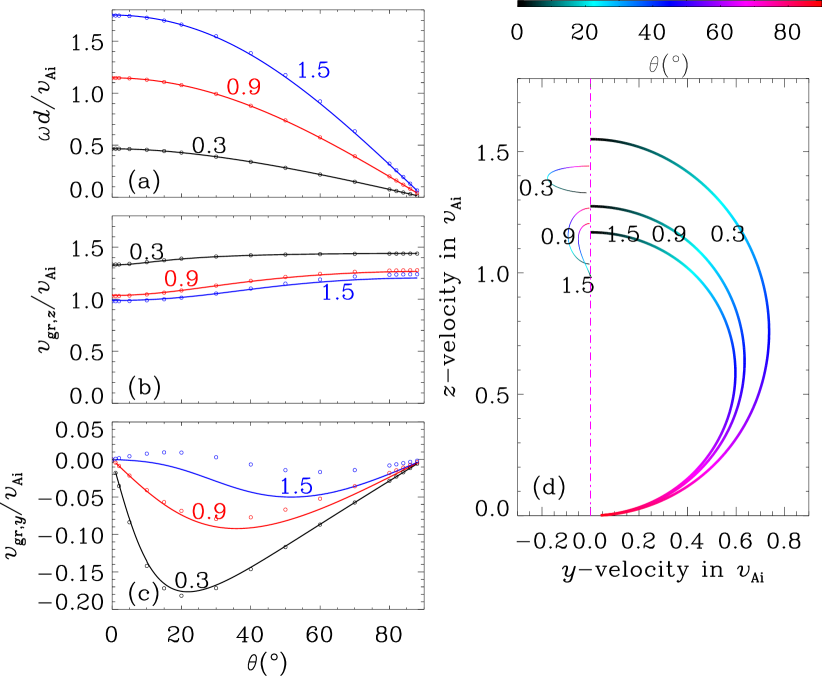
Figure 1: Dispersion properties of oblique kink modes in a slab equilibrium structured only in the $x$-direction, the density contrast (steepness parameter) being $\rho_{\rm i}/\rho_{\rm e}=3$ ($\alpha=10$). The obliqueness is measured by the angle $\theta$ between the equilibrium magnetic field $\bm{B}_{0}=B_{0}\bm{e}_{z}$ and a 2D wavevector $\bm{k}=k_{y}\bm{e}_{y}+k_{z}\bm{e}_{z}$. Left column: Dependencies on $\theta$ of (a) the oscillation frequency $\omega$, (b) the $z$-component of the group velocity $v_{{\rm gr},z}$, and (c) the $y$-component $v_{{\rm gr},y}$. Several values of $kd$ are examined as labeled. The results for a step density profile ($\alpha\to\infty$) are represented by the symbols for comparison. Right column: Phase (the thick curves) and group (thin) diagrams for a number of $kd$ as labeled. Both diagrams are color-coded by $\theta$. The dash-dotted line represents the vertical axis in the velocity plane. See text for more details.

2.2 Phase and Group Diagrams

This subsection presents the phase and group diagrams. We start by defining a 2D wavevector $\bm{k}\coloneqq k_{y}\bm{e}_{y}+k_{z}\bm{e}_{z}$, where $k_{y}\geq 0$ and $k_{z}>0$. The wavevector is alternatively represented by $k$ and $\theta$, with $k=|\bm{k}|$ and $\theta=\angle(\bm{k},\bm{B}_{0})$. We define the phase velocity as $\bm{v}_{\rm ph}=(\omega/k)\bm{e}_{k}$ with $\bm{e}_{k}$ being the unit vector along $\bm{k}$. The group velocity, on the other hand, is defined as $\bm{v}_{\rm gr}=v_{{\rm gr},y}\bm{e}_{y}+v_{{\rm gr},z}\bm{e}_{z}$ with $v_{{\rm gr},y}=\partial\omega/\partial k_{y}$ and $v_{{\rm gr},z}=\partial\omega/\partial k_{z}$. Equation (3) then enables one to convert the $k_{y}$- and $k_{z}$-dependencies of $\omega=\Re\Omega$ into the $k$- and $\theta$-dependencies of $\bm{v}_{\rm gr}$, yielding

$$v_{{\rm gr},y}/v_{\rm Ai}=\mathcal{U}_{y}(kd,\theta),\quad v_{{\rm gr},z}/v_{\rm Ai}=\mathcal{U}_{z}(kd,\theta).$$ (4)

We largely focus on how $\bm{v}_{\rm ph}$ or $\bm{v}_{\rm gr}$ varies with $\theta$, for which purpose $\omega$, $v_{{\rm gr},z}$ and $v_{{\rm gr},y}$ for the chosen $[\rho_{\rm i}/\rho_{\rm e},\alpha]=[3,10]$ are plotted against $\theta$ by the solid curves in Figures 1a to 1c. A number of $kd$ are examined as labeled. The step results ($\alpha\to\infty$) are additionally presented by the symbols. One sees that the finite $\alpha$ curves differ appreciably from the symbols only for $v_{{\rm gr},y}$ when $kd=1.5$. This is understandable because kink modes with larger $k$ possess shorter spatial scales, and therefore sense the finite inhomogeneity scale more readily. Our point, however, is that the finite $\alpha$ results can be largely understood with the step ones, for which some analytical progress is possible. This practice proves necessary given the rather involved $\theta$-dependencies, those of $v_{{\rm gr},y}$ in particular. We proceed to define

$$\kappa^{2}_{\rm i,e}=k_{z}^{2}-\dfrac{\omega^{2}}{v^{2}_{\rm Ai,e}},\quad m^{2}_{\rm i,e}=k_{y}^{2}+\kappa^{2}_{\rm i,e},$$ (5)

where $m_{\rm i,e}$ acts as some effective $x$-wavenumber for oblique kink modes (e.g., Equation (15) in Y21). We note that $m_{\rm e}^{2}$ is positive by construction, whereas $m_{\rm i}^{2}$ may be negative for small $k_{y}$ (A07, Figure 2). We take $\arg m_{\rm i}=\pi/2$ when $m_{\rm i}^{2}<0$ without loss of generality. A dispersion relation (DR) then writes (e.g., ; )

$$\coth(m_{\rm i}d)=-\dfrac{\kappa_{\rm i}^{2}}{\kappa_{\rm e}^{2}}\frac{m_{\rm e}}{m_{\rm i}}.$$ (6)

The dispersion behavior at large $\theta$ can be explained with Equation (6) by assuming $m_{\rm i}\approx m_{\rm e}\approx k_{y}$. It was first shown by Tatsuno & Wakatani (1998) in fusion contexts that

$$\omega\approx k_{z}C(k_{y}),\quad C^{2}(k_{y})=v_{\rm Ai}^{2}\dfrac{1+\tanh(k_{y}d)}{\rho_{\rm e}/\rho_{\rm i}+\tanh(k_{y}d)},$$ (7)

which was put in current form by Y21. Note that Equation (7) can also be found by imposing the incompressibility condition from the outset, with the physical reasons well documented for cylindrical equilibria (e.g., Goossens et al., 2009; Goossens et al., 2012; Soler & Terradas, 2015). Note further that Equation (7) leads to $\kappa^{2}_{\rm e}<|\kappa^{2}_{\rm i}|$, meaning that its range of validity $k_{y}^{2}\gg|\kappa^{2}_{\rm i,e}|$ becomes

$$k_{y}^{2}[\rho_{\rm e}/\rho_{\rm i}+\tanh(k_{y}d)]\gg k_{z}^{2}(1-\rho_{\rm e}/\rho_{\rm i}).$$ (8)

Evidently, $\omega\to 0$ and hence $v_{\rm ph}\to 0$ when $\theta\to 90^{\circ}$. Furthermore, one recognizes that $C(k_{y})$ decreases monotonically with $k_{y}$, meaning that $c_{\rm k}=v_{\rm Ai}\sqrt{2/(1+\rho_{\rm e}/\rho_{\rm i})}<C(k_{y})<v_{\rm Ai}\sqrt{\rho_{\rm i}/\rho_{\rm e}}=v_{\rm Ae}$ with $c_{\rm k}$ being the kink speed. Consequently, the asymptotic value of $v_{{\rm gr},z}$ at $\theta\to 90^{\circ}$ decreases monotonically with $k$, lying between $c_{\rm k}$ and $v_{\rm Ae}$. Likewise, $v_{{\rm gr},y}$ approaches zero from below. These step expectations are reproduced exactly by the symbols, explaining the finite $\alpha$ results almost quantitatively as well.

We further employ Equation (6) to understand how $v_{{\rm gr},y}$ behaves at small $\theta$. Let $\hat{\omega}$ denote $\mathcal{W}(k_{y}=0,k_{z})$ (see Equation (3) with $\alpha\to\infty$). Consider a slightly different pair $[k_{y},k_{z}]$ with $k_{y}^{2}/k^{2}_{z}\ll 1$. We see only $k_{y}$ as variable, and Taylor-expand all terms in Equation (6) about $k_{y}=0$. Some lengthy algebra yields that

$$\omega(k_{y},k_{z})\approx\hat{\omega}\left[1-\dfrac{1}{2}\dfrac{1/(\hat{\kappa}_{\rm e}d)-1}{(\hat{\omega}d/v_{\rm Ai})^{2}+(k_{z}d)^{2}/(\hat{\kappa}_{\rm e}d)}(k_{y}d)^{2}\right],$$ (9)

with $\hat{\kappa}_{\rm e}$ defined by $\hat{\kappa}^{2}_{\rm e}=k_{z}^{2}-\hat{\omega}^{2}/v_{\rm Ae}^{2}$. Note that $\hat{\kappa}^{2}_{\rm e}>0$. Equation (9) indicates that the $k_{y}$-correction is only quadratic, meaning that $v_{{\rm gr},y}\to 0$ when $\theta\to 0$. For a fixed small $\theta$, one further deduces that $v_{{\rm gr},y}$ remains negative for small $kd$ until reversing its sign when $kd$ exceeds some critical value. To explain this, we recall the textbook result that $\hat{\omega}/k_{z}$ decrease monotonically with $k_{z}$ from $v_{\rm Ae}$ at $k_{z}d\to 0$ toward $v_{\rm Ai}$ when $k_{z}d\to\infty$ (e.g., Roberts, 2019, Section 5.5.5). Now that $(\hat{\kappa}_{\rm e}d)^{2}=(k_{z}d)^{2}[1-\hat{\omega}^{2}/(k_{z}v_{\rm Ae})^{2})]$, one recognizes that $\hat{\kappa}_{e}d\ll 1$ when $k_{z}d\ll 1$ but increases monotonically with $k_{z}d$ toward large values when $k_{z}d\gg 1$. This necessarily changes the sign of $1/(\hat{\kappa}_{\rm e}d)-1$ at some $k_{z}d$, and hence a change of sign of $v_{{\rm gr},y}$. Both the curves and symbols in Figure 1c for small $\theta$ agree with the analytical expectations. Somehow different between the step and finite $\alpha$ results is that $kd=1.5$ is large enough to reverse the sign of $v_{{\rm gr},y}$ for the former but not for the latter.

Figure 1d gathers the finite $\alpha$ results to produce the phase and group diagrams, namely the trajectories that $\bm{v}_{\rm ph}=(v_{{\rm ph},y},v_{{\rm ph},z})$ (the thick curves) and $\bm{v}_{\rm gr}=(v_{{\rm gr},y},v_{{\rm gr},z})$ (thin) traverse when $\theta$ varies. These curves are color-coded by $\theta$ and labeled by $kd$. A primary result of this study, Figure 1d is striking in that the trajectories for any examined $kd$ are morphologically similar to slow waves in a uniform low-beta MHD medium, despite the absence of slow waves in zero-beta MHD (see, e.g., Figure 5.4 in Goedbloed et al. 2019). By “similar” we specifically emphasize that $\bm{v}_{\rm ph}$ and $\bm{v}_{\rm gr}$ lie astride $\bm{B}_{0}=B_{0}\bm{e}_{z}$, and the group trajectories extend only to a limited angle from $\bm{B}_{0}$. We deem it important to explore the physical reasons that yield the peculiar group trajectories from the perspective of, say, restoring forces. Equally important is to explore how the group trajectories behave in other configurations, one example being those that are associated with a magnetic shear ($\bm{B}_{0}=B_{0y}(x)\bm{e}_{y}+B_{0z}(x)\bm{e}_{z}$; see e.g., Chen & Hasegawa 1974; Arregui et al. 2003 for some motivating ideas). These explorations are nonetheless left for a future work.

Figure 2 further surveys an extensive set of $[kd,\theta]$, presenting $v_{{\rm gr},y}$ and $v_{{\rm gr},z}$ as equally spaced contours colored black and red, respectively. One sees that $v_{{\rm gr},y}$ for a given $kd$ consistently approaches zero when $\theta\to 0$ or $\theta\to 90^{\circ}$, thereby attaining a local minimum at some $kd$-dependent angle $\theta_{\rm min}$. This $\theta_{\rm min}$ increases monotonically with $kd$, and $v_{{\rm gr},y}$ is subject to a global minimum in the examined range of $kd$ (see the lower-left portion). Regarding $v_{{\rm gr},z}$, one sees that the mononotonic $\theta$-dependence for a given $kd$ in Figure 1b actually persists. However, the upper-left corner indicates that $v_{{\rm gr},z}$ for a small $\theta$ will possess a nonmonotonic $kd$-dependence when $kd$ further increases. This is indeed true. We avoid this complication, for it is not specific to oblique propagation but well known for $\theta=0$ when $\alpha\to\infty$ (e.g., Nakariakov & Roberts, 1995). Rather, by Figure 2 we stress that inverting Equation (4) with a given pair $[v_{{\rm gr},y}/v_{\rm Ai},v_{{\rm gr},z}/v_{\rm Ai}]$ does not yield a unique pair $[kd,\theta]$.

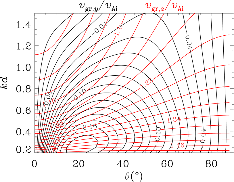
Figure 2: Distributions in the $k-\theta$ plane of the $y$- and $z$-components of the group velocity, namely $v_{{\rm gr},y}$ (the black contours) and $v_{{\rm gr},z}$ (red), for kink modes in a slab equilibrium with $[\rho_{\rm i}/\rho_{\rm e},\alpha]=[3,10]$.

3 Time-Dependent Simulation

This section examines 3D impulsively excited kink waves by numerically evolving the ideal MHD equations with the MPI-AMRVAC code (Xia et al., 2018). We prescribe the equilibrium density $\rho_{0}$ by Equation (1) with $[\rho_{\rm i}/\rho_{\rm e},\alpha]=[3,10]$. A uniform temperature $T_{0}$ is specified for simplicity, yielding a plasma beta of $0.021$ at $x=0$. We choose a $z$-directed magnetic field $\bm{B}_{0}$ whose magnitude varies with $x$ to maintain transverse force balance. This $x$-variation is nonetheless very weak, with $B_{0}$ at large $x$ being larger than that at $x=0$ by only $\sim 0.7\%$. Kink waves are excited by a perturbation

$$v_{x}(x,y,z;t=0)=v_{\rm ini}\exp\left(-\dfrac{x^{2}}{2\sigma_{x}^{2}}\right)\exp\left(-\dfrac{y^{2}}{2\sigma_{y}^{2}}\right)\exp\left(-\dfrac{z^{2}}{2\sigma_{z}^{2}}\right),$$ (10)

for which the spatial extent is chosen to be $\sigma_{x}=\sigma_{y}=\sigma_{z}=\sqrt{2}d$ and the magnitude $v_{\rm ini}$ is set to be $0.1v_{\rm Ai}$. Note that the same equilibrium was employed in the 2D study by Guo et al. (2022), and Figure 4 therein demonstrated that a magnitude $v_{\rm ini}=0.1v_{\rm Ai}$ ensures a linear behavior for the resulting kink wave train. No nonlinearity is discerned in this 3D study either, which is understandable given that nonlinearity is weaker with the introduction of the third dimension.

Our numerical setup is as follows. A subdomain $[-50,50]d\times[0,200]d\times[0,200]d$ of the full space is employed from symmetry considerations, with symmetric boundary conditions (BCs) specified at $y=0$ and $z=0$. Outflow BCs are implemented for the rest of the boundaries, where no spurious wave reflection is discerned. We adopt the second-order HLLD solver and the Woodward slope limiter when evaluating inter-cell fluxes, and choose the midpoint method for time marching with a Courant number of $0.5$. A base grid of $64\times 128\times 128$ is adopted in $(x,y,z)$. Four levels of adaptive mesh refinement (AMR) are implemented as triggered by density and velocity variations, resolving scales down to $\sim 0.19d$. Despite the symmetry considerations and the implementation of AMR, this simulation remains computationally expensive, and the chosen $\alpha=10$ is the largest we can afford to avoid spurious waves emanating from the slab boundaries.

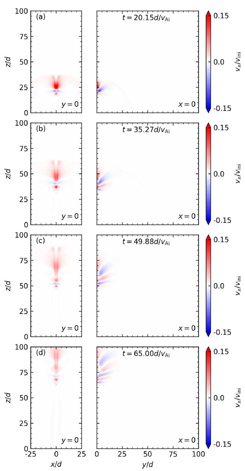
Figure 3: Snapshots of $v_{x}$ in the $y=0$ (the left column) and $x=0$ (right) planes. These images are extracted from the animation attached to this figure.

Figure 3 presents several snapshots of $v_{x}$ in the $y=0$ (the left column) and $x=0$ planes (right). The $y=0$ cuts, together with the associated animation, make it clear that the signals comprise a slab-guided component and a laterally propagating component. This lateral component, manifested as a series of circular ripples, attenuates rather rapidly and becomes difficult to discern when $t\gtrsim 30d/v_{\rm Ai}$. In contrast, the guided component persists throughout, characterized by that more ripples emerge with time and that small-scale variations tend to lag behind larger-scale ones. Two features arise in the $x=0$ cuts. First, the nominal lateral component is present as well, despite that the $x=0$ plane is inside the slab. Second, the guided component is confined to a rather narrow sector about $\bm{B}_{0}$, encompassing multiple stripes that form an intricate interference pattern.

We focus on the $x=0$ cuts, for the $y=0$ patterns are largely 2D (Guo et al., 2022, Figure 4). Neglecting finite pressure, we assume $\alpha\to\infty$ to make quantitative progress. One may write

$$v_{x}(x,y,z,t)=\int_{-\infty}^{\infty}dk_{y}\int_{-\infty}^{\infty}dk_{z}$$

$$\left\{\sum\limits_{j}\left[\mathcal{F}_{j}(x;k_{y},k_{z}){\rm e}^{\imath\left(\omega_{j}t-k_{y}y-k_{z}z\right)}\right]+{\rm improper}\right\},$$ (11)

by drawing analogy with the cylindrical study by ORT14 (see also Li et al. 2022). A spectral solution to the IVP, Equation (11) means that all values of $k_{y}$ and $k_{z}$ are involved given the localization of the initial perturbation. The summation collects all trapped modes, for which the frequency $\omega_{j}=\omega_{j}(k_{y},k_{z})$ ensures $m_{\rm e}^{2}>0$ (see Equation (5)). The “improper” part incorporates improper modes, which possess any frequency satisfying $m_{\rm e}^{2}<0$ and hence necessitate an integration over frequency. Regardless, the “lateral” component in Figure 3 is attributable to the improper contribution.

We now consider the guided component by connecting Equation (11) with the resistive EVP results encapsulated in Figures 1 and 2. Before proceeding, however, the following remarks are necessary. Firstly, the group velocity $\bm{v}_{\rm gr}$ involves only the real part ($\omega$) of the eigenfrequency $\Omega$. What a non-vanishing $\gamma=\Im\Omega$ means for an ideal computation is that the fast wave energy is transferred to localized Alfv$\acute{\rm e}$nic motions where the Alfv$\acute{\rm e}$n resonance takes place, as has been extensively demonstrated for kink modes in cylindrical equilibria (e.g., Terradas et al., 2008; Pascoe et al., 2010; Soler & Terradas, 2015). The same also happens here in that Alfv$\acute{\rm e}$nic motions can be readily discerned as enhanced velocity shear $\partial v_{y}/\partial x$ in some moving volumes in the slab boundary that accompany the strongest $v_{x}$ perturbations. Secondly, strictly speaking, our EVP analysis needs to account for the finite beta to ensure a more self-consistent application of the EVP computation to the IVP study. On top of that, implied by such an application is that resonant absorption does not significantly impact the oscillation frequency $\omega$, which may not hold in general (Soler & Terradas, 2015). Nonetheless, two reasons make us believe that this is not too serious an issue, one being that $|\gamma/\omega|$ is consistently $<0.1$ for the wavevectors examined in Figure 2, the other being related to some quantitative analysis in what follows.

Figures 4a and 4b present two zoomed-in $x=0$ cuts of $v_{x}$. A portion of the outermost $v_{x}=0$ contour is given. With this iso-phase curve we illustrate the relevance of Figure 1d to the large-time interference pattern. Key is that the method of stationary phase (MSP) is increasingly applicable as time proceeds. Suppose that the MSP applies to some $(y,z,t)$. Equation (11) is then dominated by those wavepackets (WPs) with central wavevectors $\bm{K}_{n}=K_{n,y}\bm{e}_{y}+K_{n,z}\bm{e}_{z}$ (W74, Equation (11.41)),

$$v_{x}(0,y,z,t)\sim t^{-1}\sum\limits_{n}\left[\mathcal{G}_{n}(K_{n,y},K_{n,z}){\rm e}^{\imath\left(\omega_{n}t-K_{n,y}y-K_{n,z}z\right)}\right],$$ (12)

where $\omega_{n}=\omega_{n}(\bm{K}_{n})$ with $\bm{K}_{n}$ a solution to

$$v_{{\rm gr},y}(\bm{K}_{n})=y/t,\quad v_{{\rm gr},z}(\bm{K}_{n})=z/t.$$ (13)

One complication, however, is that Equation (13) possesses two solutions even if one assumes the relevance of only those modes in Figure 2. This is illustrated in Figure 4a where the arrows represent the central wavevectors of the two WPs that solve Equation (13) for a point with $y=4d$ on the $v_{x}=0$ curve. Note that $K_{y}<0$ (see the symmetry property following Equation (3)). Let these WPs be labeled $1$ and $1^{\prime}$, and suppose that the unprimed WP dominates. Two consequences follow. First, $\bm{K}_{1}$ is locally normal to the iso-phase curve. Second, the time sequence seen by WP 1, $V_{x}(t)\coloneqq v_{x}(0,v_{{\rm gr},y}(\bm{K}_{1})t,v_{{\rm gr},z}(\bm{K}_{1})t,t)$, eventually becomes $\sim t^{-1}\sin[\varpi(\bm{K}_{1})t+\phi(\bm{K}_{1})]$ with

$$\varpi(\bm{K}_{1})=\omega(\bm{K}_{1})-K_{1,y}v_{{\rm gr},y}(\bm{K}_{1})-K_{1,z}v_{{\rm gr},z}(\bm{K}_{1})$$ (14)

being a Doppler-shifted frequency and $\phi$ some phase angle. This second property applies to any WP, and is hence useful for assessing whether the MSP applies or judging whether a WP dominates. The $V_{x}(t)t$ sequence seen by WP 1 is presented by the black solid curve in Figure 4c. A sinusoid fitting with the expected $\varpi(\bm{K}_{1})$ (the black dashed curve) strongly suggests that the MSP applies to the trajectory of WP 1 when $t\gtrsim 7d/v_{\rm Ai}$, despite the minor deviation of $\bm{K}_{1}$ from the local normal. The same practice is repeated for WP 2 in Figure 4b pertinent to a point with $y=4d$ on the solid curve. Now the MSP applies for $t\gtrsim 10d/v_{\rm Ai}$ (see the blue curves in Figure 4c), and $\bm{K}_{2}$ is nearly perfectly perpendicular to the iso-phase curve. The negative $y$-propagation of the delineated $v_{x}=0$ front may therefore be accounted for by the dispersion features in Figure 1d.

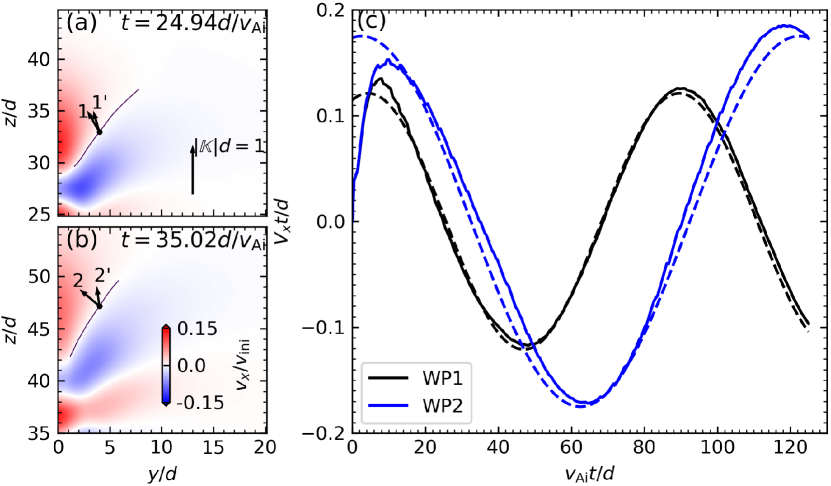
Figure 4: Left: Snapshots of $v_{x}$ in the $x=0$ plane at two labeled instants. The solid curve in each panel is part of the outermost $v_{x}=0$ contour, the arrows representing the central wavevectors of the two wavepackets expected for the location chosen on this iso-phase curve. The vertical arrow measures the magnitude of any wavevector. Right: The time sequence of $v_{x}t$ sampled by an observer moving with wavepacket $1$ (the black solid curve) or wavepacket $2$ (blue). Each sequences is fitted with a sinusoid incorporating expectations from linear theory (the dashed curve). See text for details.

4 Summary

This study examined the three-dimensional (3D) propagation of kink wave trains impulsively excited by a localized perturbation to straight, field-aligned, symmetric, coronal slabs that are structured only in one transverse direction. Two features stand out in our linear EVP analysis on oblique kink modes, namely the group and phase velocities may lie astride the equilibrium magnetic field ($\bm{B}_{0}$), and the group trajectories extend only to a limited angle from $\bm{B}_{0}$. These features were demonstrated numerically for continuous and step structuring alike, and were understood with the approximate analytical expressions enabled by the latter. Our 3D time-dependent simulation showed that these features are reflected in the intricate interference patterns at large times, the key being the ideas behind the method of stationary phase. The guided wave trains in the out-of-plane cut through the slab axis are confined to a narrow sector about $\bm{B}_{0}$, with some wavefronts propagating toward $\bm{B}_{0}$.

Data Availability

The data underlying this article are available in the article and in its references.

References

- Arregui et al. (2003) Arregui I., Oliver R., Ballester J. L., 2003, A&A, 402, 1129
- Arregui et al. (2007) Arregui I., Terradas J., Oliver R., Ballester J. L., 2007, Sol. Phys., 246, 213
- Chen & Hasegawa (1974) Chen L., Hasegawa A., 1974, Physics of Fluids, 17, 1399
- Goedbloed et al. (2019) Goedbloed H., Keppens R., Poedts S., 2019, Magnetohydrodynamics of Laboratory and Astrophysical Plasmas. Cambridge University Press, doi:10.1017/9781316403679
- Goossens et al. (1992) Goossens M., Hollweg J. V., Sakurai T., 1992, Sol. Phys., 138, 233
- Goossens et al. (2009) Goossens M., Terradas J., Andries J., Arregui I., Ballester J. L., 2009, A&A, 503, 213
- Goossens et al. (2011) Goossens M., Erdélyi R., Ruderman M. S., 2011, Space Sci. Rev., 158, 289
- Goossens et al. (2012) Goossens M., Andries J., Soler R., Van Doorsselaere T., Arregui I., Terradas J., 2012, ApJ, 753, 111
- Guo et al. (2022) Guo M., Li B., Van Doorsselaere T., Shi M., 2022, MNRAS, 515, 4055
- Hasegawa & Chen (1974) Hasegawa A., Chen L., 1974, Phys. Rev. Lett., 32, 454
- Ionson (1978) Ionson J. A., 1978, ApJ, 226, 650
- Kolotkov et al. (2021) Kolotkov D. Y., Nakariakov V. M., Moss G., Shellard P., 2021, MNRAS, 505, 3505
- Li et al. (2018) Li B., Guo M.-Z., Yu H., Chen S.-X., 2018, ApJ, 855, 53
- Li et al. (2022) Li B., Chen S.-X., Li A.-L., 2022, ApJ, 928, 33
- Murawski & Roberts (1993) Murawski K., Roberts B., 1993, Sol. Phys., 144, 101
- Nakariakov & Kolotkov (2020) Nakariakov V. M., Kolotkov D. Y., 2020, ARA&A, 58, 441
- Nakariakov & Roberts (1995) Nakariakov V. M., Roberts B., 1995, Sol. Phys., 159, 399
- Nakariakov & Verwichte (2005) Nakariakov V. M., Verwichte E., 2005, Living Reviews in Solar Physics, 2, 3
- Nakariakov et al. (2021) Nakariakov V. M., et al., 2021, Space Sci. Rev., 217, 73
- Ogrodowczyk & Murawski (2006) Ogrodowczyk R., Murawski K., 2006, Sol. Phys., 236, 273
- Oliver et al. (2014) Oliver R., Ruderman M. S., Terradas J., 2014, ApJ, 789, 48
- Pascoe et al. (2010) Pascoe D. J., Wright A. N., De Moortel I., 2010, ApJ, 711, 990
- Pascoe et al. (2013) Pascoe D. J., Nakariakov V. M., Kupriyanova E. G., 2013, A&A, 560, A97
- Poedts & Kerner (1991) Poedts S., Kerner W., 1991, Phys. Rev. Lett., 66, 2871
- Roberts (2000) Roberts B., 2000, Sol. Phys., 193, 139
- Roberts (2008) Roberts B., 2008, in Erdélyi R., Mendoza-Briceno C. A., eds, Vol. 247, Waves & Oscillations in the Solar Atmosphere: Heating and Magneto-Seismology. pp 3–19, doi:10.1017/S1743921308014609
- Roberts (2019) Roberts B., 2019, MHD Waves in the Solar Atmosphere. Cambridge University Press, doi:10.1017/9781108613774
- Roberts et al. (1983) Roberts B., Edwin P. M., Benz A. O., 1983, Nature, 305, 688
- Roberts et al. (1984) Roberts B., Edwin P. M., Benz A. O., 1984, ApJ, 279, 857
- Ruderman et al. (1995) Ruderman M. S., Tirry W., Goossens M., 1995, Journal of Plasma Physics, 54, 129
- Sewell (1988) Sewell G., 1988, The Numerical Solution of Ordinary and Partial Differential Equations. San Diego: Academic Press
- Soler & Terradas (2015) Soler R., Terradas J., 2015, ApJ, 803, 43
- Tataronis & Grossmann (1973) Tataronis J., Grossmann W., 1973, Zeitschrift fur Physik, 261, 203
- Tatsuno & Wakatani (1998) Tatsuno T., Wakatani M., 1998, Journal of the Physical Society of Japan, 67, 2322
- Terradas et al. (2006) Terradas J., Oliver R., Ballester J. L., 2006, ApJ, 642, 533
- Terradas et al. (2008) Terradas J., Andries J., Goossens M., Arregui I., Oliver R., Ballester J. L., 2008, ApJ, 687, L115
- Uchida (1970) Uchida Y., 1970, PASJ, 22, 341
- Wentzel (1979) Wentzel D. G., 1979, ApJ, 227, 319
- Whitham (1974) Whitham G., 1974, Linear and Nonlinear Waves. New York: Wiley, https://books.google.nl/books?id=f8oRAQAAIAAJ
- Xia et al. (2018) Xia C., Teunissen J., El Mellah I., Chané E., Keppens R., 2018, ApJS, 234, 30
- Yu et al. (2021) Yu H., Li B., Chen S., Guo M., 2021, Sol. Phys., 296, 95