Layer-wise shared attention network on dynamical system perspective

Abstract

Attention networks have successfully boosted accuracy in various vision problems. Previous works lay emphasis on designing a new self-attention module and follow the traditional paradigm that individually plugs the modules into each layer of a network. However, such a paradigm inevitably increases the extra parameter cost with the growth of the number of layers. From the dynamical system perspective of the residual neural network, we find that the feature maps from the layers of the same stage are homogenous, which inspires us to propose a novel-and-simple framework, called the dense and implicit attention (DIA) unit, that shares a single attention module throughout different network layers. With our framework, the parameter cost is independent of the number of layers and we further improve the accuracy of existing popular self-attention modules with significant parameter reduction without any elaborated model crafting. Extensive experiments on benchmark datasets show that the DIA is capable of emphasizing layer-wise feature interrelation and thus leads to significant improvement in various vision tasks, including image classification, object detection, and medical application. Furthermore, the effectiveness of the DIA unit is demonstrated by novel experiments where we destabilize the model training by (1) removing the skip connection of the residual neural network, (2) removing the batch normalization of the model, and (3) removing all data augmentation during training. In these cases, we verify that DIA has a strong regularization ability to stabilize the training, i.e., the dense and implicit connections formed by our method can effectively recover and enhance the information communication across layers and the value of the gradient thus alleviate the training instability.

1 Introduction

Attention, a cognitive process that selectively focuses on a small part of information while neglects other perceivable information [1, 2], has been used to effectively ease neural networks from learning large information contexts from sentences [3, 4, 5], images [6, 7] and videos [8]. Especially in computer vision, deep neural networks (DNNs) incorporated with special operators that mimic the attention mechanism can process informative regions of an image efficiently. These operators are modularized and plugged into networks as attention modules [9, 10, 11, 12, 13, 14]. Generally, the self-attention module can be divided into three parts: “extraction”, “processing” and “recalibration” like Figure 1. First, the plug-in module extracts internal features of a network which can be squeezed as the channel-wise information [9, 15], spatial information [12, 10, 11], etc. Next, the module processes the extraction and generates an attention map to measure the importance of the features map via a fully connected layer [9], convolution layer [12], etc. Last, the attention map is applied to recalibrate the features. Most existing works adpot a common paradigm where the attention modules are individually plugged into each block throughout DNNs [9, 10, 11, 12]. This paradigm facilitates researchers to focus on the optimization of three parts in SAM and allows a fair and fast comparison of the performance of the designed modules, which has greatly advanced the community.

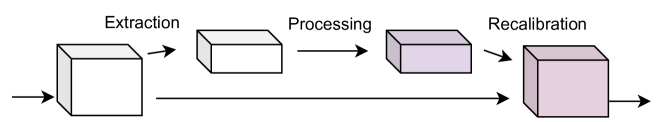
Figure 1: The paradigm of self-attention module.

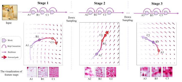
Figure 2: The Residual neural network on dynamical system perspective. The forward process of ResNet can be modeled as a forward numerical method for a dynamical system. The feature map of any block in the same stage can be regarded as a point in the same vector space. For example, in Stage 1, “A1”, “B1” and “C1” are the feature maps from three adjacent blocks, and these feature maps are homogenous.

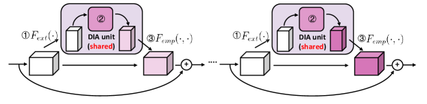
Figure 3: DIA units in the residual network. $F_{ext}$ means the operation for extracting different scales of features. $F_{emp}$ means the operation for emphasizing or recalibrating features.

However, the drawbacks of such a paradigm are obvious, i.e., the computation and memory create a bottleneck with the increasing numbers of SAMs. Specifically, for DNNs, the performance and depth are closely related. Under a suitable training setting, deeper networks can achieve better performance. This empirical phenomenon reveals that if we connect the SAMs individually with each block of the entire DNN backbone for granted, then this will inevitably lead to increasing computational cost and numbers of parameters with the growth of network depth. Considering these practical issues, it is necessary and essential to ask a question:

Do we really need to set up so many self-attention modules for every layer in a neural network?

To answer this question fundamentally, we first consider the dynamical system perspective of residual neural networks (ResNets), which successfully explains some behaviors of DNNs and improves the performance of the model. In general, as shown in Table I, the forward process of ResNet can be modeled as a forward numerical method for a dynamical system as Eq.(1).

$$\frac{\text{d}\mathbf{u}}{\text{d}t}=\mathbf{f}(\mathbf{u}),\quad\mathbf{u}(0)=\mathbf{c}_{0},$$ (1)

where $\mathbf{c}_{0}$ represents an initial condition, which corresponds to the input in the residual network and $\mathbf{u}(t)\equiv\mathbf{u}_{t}$ is a time-dependent $d$-dimensional state, which is used to describe the input feature $x_{t}$ of $t^{\rm th}$ block. The neural network $f(\cdot;\theta_{t})$ with learnable parameters $\theta_{t}$ in $t^{\rm th}$ block can be regarded as a integration $S(\cdot;\mathbf{f},\Delta t)$ with step $\Delta t$ and numerical method $S$. Some existing works [16, 17, 18, 19, 20] consider that since for the state $\mathbf{u}_{t}$, the numerical methods always are the same integration method $S$ for solving Eq.(1), thus they also use the block shared with the same parameters to process the input $x_{t}$ in ResNet. This design forms the ResNet as a recurrent structure, and with a suitable training setup, such a structure can achieve a relatively good performance while the number of parameters of the model can be greatly reduced.

TABLE I: The dynamical system perspective for residual neural networks.

Dynamical system	ResNet
$\mathbf{u}_{t+1}=\mathbf{u}_{t}+S(\mathbf{u}_{t};\mathbf{f},\Delta t)$	$x_{t+1}=x_{t}+f(x_{t};\theta_{t})$

Based on this view, as shown in Figure 2, the feature map of any block in the same stage (the collection of successive layers with the same spatial size) can be regarded as a point in the same vector space, since they are fed by a same neural network $f(\cdot;\theta_{t})$, i.e. these feature maps belong to a same domain of a function. Therefore, the feature maps in each vector space can be considered as homogenous, which means we can naturally use only one self-attention module $\mathbf{A}(\cdot;{\color[rgb]{1,0,0}\phi_{\text{share}}})$ for feature map $f(x_{t};\theta_{t})$ as

$$x_{t+1}=x_{t}+\underbrace{f(x_{t};\theta_{t})}_{\text{Feature map}}\otimes\underbrace{\mathbf{A}(f(x_{t};\theta_{t});{\color[rgb]{1,0,0}\phi_{\text{share}}})}_{\text{Attention map}},$$ (2)

instead of customizing self-attention modules $\mathbf{A}(\cdot;\phi_{t})$ for each block, as in Eq. (3). Moreover, for the feature maps from different stages, since the dimensions of the feature maps in different stages are different (e.g., for ResNet164, the dimensions of three stages are $(64\times 32\times 32)$, $(128\times 16\times 16)$ and $(256\times 8\times 8)$, respectively) and they are generally considered to contain different information from low level to high level [21, 22]. Therefore, the features from different stages are usually supposed to be heterogeneous, which can be intuitively verified from the visualization of the feature maps in Figure 2, e.g., in different stages, “A1”, “A2” and “A3” look quite different.

$$x_{t+1}=x_{t}+\underbrace{f(x_{t};\theta_{t})}_{\text{Feature map}}\otimes\underbrace{\mathbf{A}(f(x_{t};\theta_{t});\phi_{t})}_{\text{Attention map}}.$$ (3)

According to the above analyses, in the present work, we take a step forward toward efficient parameter sharing that we propose a novel-and-simple framework, i.e., sharing a self-attention module throughout different network layers to encourage the integration of layer-wise information, and this parameter-sharing module is referred to as dense-and-implicit-Attention (DIA) unit.

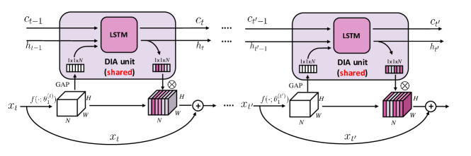
Figure 4: The showcase of DIA-LSTM. In the LSTM cell, $c_{t}$ is the cell state vector and $h_{t}$ is the hidden state vector. GAP means global average pool over channels and $\otimes$ means channel-wise multiplication.

The structure and computation flow of a DIA unit is visualized in Figure 3. There are also three parts: extraction (\raisebox{-.9pt}{1}⃝), processing (\raisebox{-.9pt}{2}⃝) and recalibration (\raisebox{-.9pt}{3}⃝) in the DIA unit. The \raisebox{-.9pt}{2}⃝ is the main module in the DIA unit to model network attention and is the key innovation of the proposed method where the parameters of the attention module are shared among different channels and blocks.

In Section 4, we verify the performance of the DIA unit for several popular self-attention modules [9, 23, 10, 24, 25]. Our experiments show that DIA can significantly reduce the number of parameters in these modules on different backbones and datasets, while achieving competitive performance improvement without any elaborated model crafting. These results extensively demonstrate the versatility of the DIA unit. Moreover, to verify the versatility of our method across different artificial intelligence tasks and its transferability for the downstream tasks, in Section 5, we consider several benchmarks for DIA-LSTM, a kind of novel DIA architecture called DIA-LSTM, including image classification, object detection, and a medical application. Further experiments reveal that DIA-LSTM can consistently improve the performance of the model in different tasks. Furthermore, we conduct the ablation studies for DIA-LSTM in Section 6 and analyze how DIA benefits the training in Section 7. Specifically, we destabilize the model training by (1) removing the skip connection of the residual neural network, (2) removing the batch normalization of the model, or (3) removing all data augmentation during training. In these cases, we verify that the dense and implicit connections formed by our method can effectively emphasize layer-wise feature interrelation, which can recover and enhance the information communication across layers and the value of the gradient thus alleviating the training instability. Finally, we have a discussion for DIA-LSTM.

2 Our contribution

We summarize our contribution as follows,

1. Inspired by the dynamical system perspective of ResNet, we propose a novel-and-simple framework that shares a self-attention module throughout different network layers to encourage the integration of layer-wise information. This framework can enhance the performance of the existing self-attention modules while the number of parameters of the models can be significantly reduced.

2. We propose incorporating LSTM in the DIA unit (DIA-LSTM) and show the effectiveness of DIA-LSTM for several vision tasks by conducting experiments on benchmark datasets and popular networks.

3. We conduct comprehensive experiments and find that our method can establish the dense and implicit connections between the self-attention modules and backbone network, leading to stable training for the neural networks.

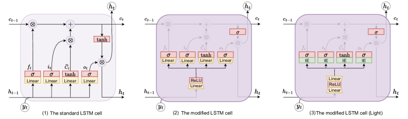
Figure 5: Left. The standard LSTM cell. Middle. The modified LSTM cell in DIA unit. We highlight the modified component in the modified LSTM. “$\sigma$” means the sigmoid activation. “Linear” means the linear transformation. Right. A light-weight LSTM cell in the DIA unit. “IE” is a simple linear transformation as Eq.(5).

3 Related Works

3.1 Attention Mechanism in Computer Vision.

Previous works use the attention mechanism in image classification via utilizing a recurrent neural network to select and process local regions at high-resolution sequentially [26, 27, 28, 29]. Concurrent attention-based methods tend to construct operation modules to capture non-local information in an image [12, 14], and model the interrelationship between channel-wise features [9, 13]. The combination of multi-level attention is also widely studied [11, 10, 30, 31]. Prior works [32, 12, 33, 9, 13, 11, 10, 30] usually insert an attention module in each layer individually. In this work, the DIA unit is innovatively shared for all the layers in the same stage of the network, and the existing attention modules can be composited into the DIA unit readily. Besides, we adopt a global average pooling in part \raisebox{-.9pt}{1}⃝ to extract global information and a channel-wise multiplication in part \raisebox{-.9pt}{3}⃝ to recalibrate features, which is similar to SENet [9].

TABLE II: Formulation for the structure of ResNet, SENet and DIA-LSTM. $f$ is the neural network in $t^{\rm th}$ block with learnable parameters $\theta_{t}$. $\text{GAP}(\cdot)$ means global average pooling. FC means fully connected layer, and $\phi_{t}$ is the trainable parameter within the SE module at the $t^{\rm th}$ layer.

	ResNet	SENet [9]	DIA-LSTM (ours)
(a)	$a_{t}=f(x_{t};\theta_{t})$	$a_{t}=f(x_{t};\theta_{t})$	$a_{t}=f(x_{t};\theta_{t})$
(b)	-	$h_{t}=\text{FC}(\text{GAP}(a_{t});\phi_{t})$	$(h_{t},c_{t})=\text{LSTM}(\text{GAP}(a_{t}),h_{t-1},c_{t-1};\phi_{\text{share}})$
(c)	$x_{t+1}=x_{t}+a_{t}$	$x_{t+1}=x_{t}+a_{t}\otimes h_{t}$	$x_{t+1}=x_{t}+a_{t}\otimes h_{t}$

3.2 Dense Network Topology.

DenseNet proposed in [34] connects all pairs of layers directly with an identity map. Through reusing features, DenseNet has the advantage of higher parameter efficiency, a better capacity of generalization, and more accessible training than alternative architectures [35, 36, 37, 38]. Instead of explicitly dense connections, the DIA unit implicitly links layers at different depths via a shared module and leads to dense connections.

3.3 Multi-Dimension Feature Integration.

L. Wolf et al[39] experimentally analyze that even the simple aggregation of low-level visual features sampled from a wide inception field can be efficient and robust for context representation, which inspires [9, 13] to incorporate multi-level features to improve the network representation. H. Li et al[40] also demonstrate that by biasing the feature response in each convolutional layers using different activation functions, the deeper layer could achieve the better capacity of capturing the abstract pattern in DNN. In the DIA unit, the high non-linearity relationship between multidimensional features is learned and integrated via the LSTM module.

TABLE III: The performance of the several existing self-attention modules with and without DIA. “Org” denotes the backbone without any self-attention module. $r$ and $k$ are the hyper-parameters for SE and ECA. $\dagger$ When SRM is applied to DIA unit, the batch normalization is not shared in stage, which will be discussed in Section 7.3. The p-value ($p$) is the Student’s t-test between the accuracies of the self-attention modules with and without DIA. The significance level $\alpha$ is 0.05. Notation: “*”: $p<0.05$. Red color means the accuracy can be improved with DIA, and Green color indicates performance degradation.

Model	Dataset	Backbone	Top1-acc.	Top1-acc. with DIA	p-value
Org	CIFAR10	ResNet83	93.62$\pm$ 0.20	-	N/A
SE $(r=4)$ [9]	CIFAR10	ResNet83	94.20$\pm$ 0.16	94.32$\pm$ 0.11 ($\uparrow$ 0.12)	*
SE $(r=8)$ [9]	CIFAR10	ResNet83	93.82$\pm$ 0.22	94.02$\pm$ 0.16 ($\uparrow$ 0.20)	*
SE $(r=16)$ [9]	CIFAR10	ResNet83	93.42$\pm$ 0.18	93.92$\pm$ 0.07 ($\uparrow$ 0.50)	*
SE $(r=32)$ [9]	CIFAR10	ResNet83	93.22$\pm$ 0.15	93.54$\pm$ 0.27 ($\uparrow$ 0.32)	*
ECA $(k=5)$ [23]	CIFAR10	ResNet83	93.32$\pm$ 0.23	93.58$\pm$ 0.15 ($\uparrow$ 0.26)	*
ECA $(k=7)$ [23]	CIFAR10	ResNet83	93.67$\pm$ 0.16	93.83$\pm$ 0.22 ($\uparrow$ 0.26)	*
ECA $(k=9)$ [23]	CIFAR10	ResNet83	94.01$\pm$ 0.32	94.12$\pm$ 0.37 ($\uparrow$ 0.11)	*
CBAM [10]	CIFAR10	ResNet83	93.31$\pm$ 0.32	93.01$\pm$ 0.44 ($\downarrow$ 0.30)	*
SRM$\dagger$ [24]	CIFAR10	ResNet83	94.22$\pm$ 0.14	94.41$\pm$ 0.13 ($\uparrow$ 0.19)	*
SPA [25]	CIFAR10	ResNet83	94.52$\pm$ 0.14	94.81$\pm$ 0.22 ($\uparrow$ 0.29)	*
Org	CIFAR10	ResNet164	93.16$\pm$ 0.15	-	N/A
SE $(r=4)$ [9]	CIFAR10	ResNet164	94.32$\pm$ 0.20	94.62$\pm$ 0.11 ($\uparrow$ 0.30)	*
SE $(r=8)$ [9]	CIFAR10	ResNet164	94.25$\pm$ 0.16	94.82$\pm$ 0.09 ($\uparrow$ 0.57)	*
SE $(r=16)$ [9]	CIFAR10	ResNet164	93.92$\pm$ 0.11	94.42$\pm$ 0.22 ($\uparrow$ 0.50)	*
SE $(r=32)$ [9]	CIFAR10	ResNet164	94.03$\pm$ 0.08	94.67$\pm$ 0.15 ($\uparrow$ 0.64)	*
ECA $(k=5)$ [23]	CIFAR10	ResNet164	94.47$\pm$ 0.12	94.87$\pm$ 0.17 ($\uparrow$ 0.40)	*
ECA $(k=7)$ [23]	CIFAR10	ResNet164	94.16$\pm$ 0.13	94.76$\pm$ 0.09 ($\uparrow$ 0.60)	*
ECA $(k=9)$ [23]	CIFAR10	ResNet164	94.52$\pm$ 0.06	94.77$\pm$ 0.15 ($\uparrow$ 0.25)	*
CBAM [10]	CIFAR10	ResNet164	93.82$\pm$ 0.11	94.63$\pm$ 0.05 ($\uparrow$ 0.81)	*
SRM$\dagger$ [24]	CIFAR10	ResNet164	94.52$\pm$ 0.21	94.75$\pm$ 0.10 ($\uparrow$ 0.24)	*
SPA [25]	CIFAR10	ResNet164	94.22$\pm$ 0.14	94.76$\pm$ 0.10 ($\uparrow$ 0.54)	*
Org	CIFAR100	ResNet83	73.55$\pm$ 0.34	-	N/A
SE $(r=4)$ [9]	CIFAR100	ResNet83	74.68$\pm$ 0.36	74.89$\pm$ 0.38 ($\uparrow$ 0.21)	*
SE $(r=8)$ [9]	CIFAR100	ResNet83	74.83$\pm$ 0.16	75.03$\pm$ 0.10 ($\uparrow$ 0.20)	*
SE $(r=16)$ [9]	CIFAR100	ResNet83	74.54$\pm$ 0.21	75.19$\pm$ 0.16 ($\uparrow$ 0.65)	*
SE $(r=32)$ [9]	CIFAR100	ResNet83	74.46$\pm$ 0.12	74.90$\pm$ 0.22 ($\uparrow$ 0.44)	*
ECA $(k=5)$ [23]	CIFAR100	ResNet83	74.54$\pm$ 0.37	74.75$\pm$ 0.09 ($\uparrow$ 0.21)	*
ECA $(k=7)$ [23]	CIFAR100	ResNet83	74.98$\pm$ 0.17	75.32$\pm$ 0.17 ($\uparrow$ 0.34)	*
ECA $(k=9)$ [23]	CIFAR100	ResNet83	75.04$\pm$ 0.26	75.15$\pm$ 0.16 ($\uparrow$ 0.11)	*
CBAM [10]	CIFAR100	ResNet83	73.24$\pm$ 0.20	73.83$\pm$ 0.25 ($\uparrow$ 0.59)	*
SRM$\dagger$ [24]	CIFAR100	ResNet83	74.48$\pm$ 0.33	74.70$\pm$ 0.25 ($\uparrow$ 0.22)	*
SPA [25]	CIFAR100	ResNet83	75.18$\pm$ 0.25	75.68$\pm$ 0.28 ($\uparrow$ 0.50)	*
Org	CIFAR100	ResNet164	74.32$\pm$ 0.22	-	N/A
SE $(r=4)$ [9]	CIFAR100	ResNet164	75.23$\pm$ 0.18	75.95$\pm$ 0.15 ($\uparrow$ 0.62)	*
SE $(r=8)$ [9]	CIFAR100	ResNet164	75.13$\pm$ 0.07	75.83$\pm$ 0.10 ($\uparrow$ 0.70)	*
SE $(r=16)$ [9]	CIFAR100	ResNet164	75.32$\pm$ 0.14	75.92$\pm$ 0.09 ($\uparrow$ 0.60)	*
SE $(r=32)$ [9]	CIFAR100	ResNet164	75.06$\pm$ 0.13	75.85$\pm$ 0.15 ($\uparrow$ 0.79)	*
ECA $(k=5)$ [23]	CIFAR100	ResNet164	74.15$\pm$ 0.36	74.57$\pm$ 0.25 ($\uparrow$ 0.42)	*
ECA $(k=7)$ [23]	CIFAR100	ResNet164	74.23$\pm$ 0.28	74.38$\pm$ 0.20 ($\uparrow$ 0.15)	*
ECA $(k=9)$ [23]	CIFAR100	ResNet164	74.88$\pm$ 0.38	75.18$\pm$ 0.31 ($\uparrow$ 0.30)	*
CBAM [10]	CIFAR100	ResNet164	73.68$\pm$ 0.21	73.82$\pm$ 0.14 ($\uparrow$ 0.14)	*
SRM$\dagger$ [24]	CIFAR100	ResNet164	74.95$\pm$ 0.67	74.69$\pm$ 0.64 ($\downarrow$ 0.26)	*
SPA [25]	CIFAR100	ResNet164	75.36$\pm$ 0.28	75.93$\pm$ 0.34 ($\uparrow$ 0.57)	*

4 Dense-and-Implicit-Attention

4.1 DIA unit for different self-attention module

In this section, we compare several existing self-attention modules, including SE [9], ECA [23], CBAM [10], SRM [24] and SPA [25], with and without DIA unit on CIFAR10/CIFAR100 datasets.

For these modules, ResNet83 and ResNet164 are used as the backbone model, and each model is trained 164 epochs with batch size of 128. The initial learning rates were set as 0.1 and decayed by a factor of 10 at the 81^th and the 122^th epochs. We adopt the stochastic gradient descent (SGD) optimizer with 0.9 momentum and $1\times 10^{-4}$ weight decay values. The results are shown in Table III where all models are verified 15 times with random seeds and the mean value and the standard deviations of the classification accuracies are reported.

In Table III, for these self-attention modules with different hyper-parameters, our framework can significantly reduce the number of parameters while maintaining the performance of these models without DIA. The number of parameters of each self-attention module can be reduced by 94.4% and 88.9% with ResNet164 and ResNet83, respectively. Next, since the batch normalization is not shared in the stage for SRM (see Section 7.3), the number of parameters of SRM can be reduced by about 40%. Moreover, most of these modules with DIA can have significant accuracy improvement (p-value$<0.05$), and a small number of them have a small performance loss under several settings. Note that some modules are not specifically designed for specific datasets CIFAR datasets in their original paper. In Table III, we reproduce these modules on CIFAR10/CIFAR100, and although the performance of some of them is not very good, it still can illustrate the effectiveness of DIA.

4.2 DIA-LSTM

The idea of parameter sharing is also used in Recurrent Neural Networks (RNN) to capture contextual information, so we consider applying RNN in our framework to model the layer-wise interrelation. Since Long Short Term Memory (LSTM) [41] is capable of capturing long-distance dependency, we mainly focus on the case when we use LSTM in DIA unit (DIA-LSTM), and the remainder of our paper studies DIA-LSTM.

Figure 4 is the showcase of DIA-LSTM. A global average pooling (GAP) layer (as the \tiny{1}⃝ in Figure 3) is used to extract global information from current layer. A LSTM module (as the \tiny{2}⃝ in Figure 3) is used to integrate multi-scale information and there are three inputs passed to the LSTM: the extracted global information from current raw feature map, the hidden state vector $h_{t-1}$, and cell state vector $c_{t-1}$ from previous layers. Then the LSTM outputs the new hidden state vector $h_{t}$ and the new cell state vector $c_{t}$. The cell state vector $c_{t}$ stores the information from the $t^{th}$ layer and its preceding layers. The new hidden state vector $h_{t}$ (dubbed as attention map in our work) is then applied back to the raw feature map by channel-wise multiplication (as the \tiny{3}⃝ in Figure 3) to recalibrate the feature. The LSTM in the DIA unit plays a role in bridging the current layer and preceding layers such that the DIA unit can adaptively learn the non-linearity relationship between features in two different dimensions. The first dimension of features is the internal information of the current layer. The second dimension represents the outer information, regarded as layer-wise information, from the preceding layers. The non-linearity relationship between these two dimensions will benefit attention modeling for the current layer. The multiple dimension modeling enables DIA-LSTM to have a regularization effect.

4.2.1 Formulation of DIA-LSTM

As shown in Figure 4 when DIA-LSTM is built with a residual network [37], the input of the $t^{\rm th}$ layer is $x_{t}\in\mathbb{R}^{W\times H\times N}$, where $W,H$ and $N$ mean width, height and the number of channels, respectively. $f(\cdot;\theta_{t})$ is the residual mapping at the $t^{\rm th}$ layer with parameters $\theta_{t}$ as introduced in [37]. Let $a_{t}=f(x_{t};\theta_{t})\in\mathbb{R}^{W\times H\times N}.$ Next, a global average pooling denoted as $\text{GAP}(\cdot)$ is applied to $a_{t}$ to extract global information from features in the current layer. Then $\text{GAP}(a_{t})\in\mathbb{R}^{N}$ is passed to LSTM along with a hidden state vector $h_{t-1}$ and a cell state vector $c_{t-1}$ ( $h_{0}$ and $c_{0}$ are initialized as zero vectors). The LSTM finally generates a current hidden state vector $h_{t}\in\mathbb{R}^{N}$ and a cell state vector $c_{t}\in\mathbb{R}^{N}$ as

$$(h_{t},c_{t})=\text{LSTM}(\text{GAP}(a_{t}),h_{t-1},c_{t-1};\phi_{\text{share}}).$$ (4)

In our model, the hidden state vector $h_{t}$ is regarded as an attention map to recalibrate feature maps adaptively. We apply channel-wise multiplication $\otimes$ to enhance the importance of features, i.e., $a_{t}\otimes h_{t}$ and obtain $x_{t+1}$ after skip connection, i.e., $x_{t+1}=x_{t}+a_{t}\otimes h_{t}$. Table II shows the formulation of ResNet, SENet [9], and DIANet, and Part (b) is the main difference between them. The LSTM module is used repeatedly and shared with different layers in parallel to the network backbone. Therefore the number of parameters $\phi_{\text{share}}$ in an LSTM does not depend on the number of layers in the backbone, e.g., $t$. SENet utilizes an attention module consisting of fully connected layers to model the channel-wise dependency for each layer individually [9]. The total number of parameters brought by the add-in modules depends on the number of layers in the backbone and increases with the number of layers.

TABLE IV: The performance of existing self-attention and our DIA-LSTM on CIFAR10/100. “Param” is the number of parameters. “Org” denotes the backbone without any self-attention module. The p-value ($p$) is the Student’s t-test between the accuracies of the DIA-LSTM and other models. The significance level $\alpha$ is 0.05. Notation: “*”: $p<0.05$. The best and the second best results of each setting are marked in bold and italic fonts, respectively. Red color means the accuracy can be improved with different modules, and Green color indicates performance degradation.

Backbone	Dataset	Model	Param	Top1-acc.	Top1-acc.↑	p-value
ResNet164	CIFAR10	Org	1.70M	93.39$\pm$ 0.23	-	*
ResNet164	CIFAR10	SE [9]	1.91M	94.32$\pm$ 0.20	0.93	*
ResNet164	CIFAR10	ECA [23]	1.70M	94.47$\pm$ 0.12	1.08	*
ResNet164	CIFAR10	CBAM [10]	1.92M	93.82$\pm$ 0.11	0.43	*
ResNet164	CIFAR10	SRM [24]	1.74M	94.52$\pm$ 0.21	1.13	*
ResNet164	CIFAR10	SPA [25]	1.93M	94.22$\pm$ 0.14	0.83	*
ResNet164	CIFAR10	SEM [42]	1.95M	94.62$\pm$ 0.23	1.23	*
ResNet164	CIFAR10	SPEM [43]	1.74M	94.81$\pm$ 0.41	1.41	*
ResNet164	CIFAR10	DIA-LSTM	1.92M	95.03$\pm$ 0.16	1.63	N/A
ResNet164	CIFAR10	DIA-LSTM (Light)	1.73M	95.19$\pm$ 0.13	1.79	*
ResNet164	CIFAR100	Org	1.73M	74.32$\pm$ 0.22	-	*
ResNet164	CIFAR100	SE [9]	1.93M	75.23$\pm$ 0.18	0.91	*
ResNet164	CIFAR100	ECA [23]	1.73M	74.15$\pm$ 0.36	-0.17	*
ResNet164	CIFAR100	CBAM [10]	1.93M	73.68$\pm$ 0.21	-0.64	*
ResNet164	CIFAR100	SRM [24]	1.76M	74.95$\pm$ 0.67	0.63	*
ResNet164	CIFAR100	SPA [25]	1.96M	75.36$\pm$ 0.28	1.04	*
ResNet164	CIFAR100	SEM [42]	1.97M	76.36$\pm$ 0.16	2.04	*
ResNet164	CIFAR100	SPEM [43]	1.76M	76.26$\pm$ 0.26	1.94	*
ResNet164	CIFAR100	DIA-LSTM	1.95M	77.09$\pm$ 0.26	2.77	N/A
ResNet164	CIFAR100	DIA-LSTM (Light)	1.75M	77.48$\pm$ 0.09	3.16	*
WRN52-4	CIFAR10	Org	12.05M	95.69$\pm$ 0.19	-	*
WRN52-4	CIFAR10	SE [9]	12.40M	95.97$\pm$ 0.25	0.28	*
WRN52-4	CIFAR10	ECA [23]	12.05M	95.79$\pm$ 0.43	0.10	*
WRN52-4	CIFAR10	CBAM [10]	12.14M	95.63$\pm$ 0.34	-0.16	*
WRN52-4	CIFAR10	SRM [24]	12.06M	95.85$\pm$ 0.45	0.16	*
WRN52-4	CIFAR10	SPA [25]	13.00M	95.93$\pm$ 0.56	0.24	*
WRN52-4	CIFAR10	SEM [42]	12.42M	95.45$\pm$ 0.31	-0.24	*
WRN52-4	CIFAR10	SPEM [43]	12.06M	95.99$\pm$ 0.37	0.20	*
WRN52-4	CIFAR10	DIA-LSTM	12.28M	96.18$\pm$ 0.13	0.49	N/A
WRN52-4	CIFAR10	DIA-LSTM (Light)	12.08M	96.09$\pm$ 0.13	0.40	*
WRN52-4	CIFAR100	Org	12.07M	79.85$\pm$ 0.21	-	*
WRN52-4	CIFAR100	SE [9]	12.42M	80.31$\pm$ 0.36	0.46	*
WRN52-4	CIFAR100	ECA [23]	12.07M	79.88$\pm$ 0.38	0.03	*
WRN52-4	CIFAR100	CBAM [10]	12.16M	79.79$\pm$ 0.63	-0.06	*
WRN52-4	CIFAR100	SRM [24]	12.09M	80.00$\pm$ 0.20	0.15	*
WRN52-4	CIFAR100	SPA [25]	13.02M	80.11$\pm$ 0.31	0.26	*
WRN52-4	CIFAR100	SEM [42]	12.44M	80.36$\pm$ 0.61	0.51	*
WRN52-4	CIFAR100	SPEM [43]	12.09M	80.72$\pm$ 0.33	0.87	*
WRN52-4	CIFAR100	DIA-LSTM	12.30M	81.02$\pm$ 0.11	1.17	N/A
WRN52-4	CIFAR100	DIA-LSTM (Light)	12.11M	80.95$\pm$ 0.33	1.10	*
ResNeXt101,8x32	CIFAR10	Org	32.09M	95.74$\pm$ 0.31	-	*
ResNeXt101,8x32	CIFAR10	SE [9]	33.98M	96.07$\pm$ 0.07	0.33	*
ResNeXt101,8x32	CIFAR10	ECA [23]	32.09M	95.99$\pm$ 0.17	0.25	*
ResNeXt101,8x32	CIFAR10	CBAM [10]	32.56M	95.80$\pm$ 0.47	0.06	*
ResNeXt101,8x32	CIFAR10	SRM [24]	32.13M	96.12$\pm$ 0.35	0.38	*
ResNeXt101,8x32	CIFAR10	SPA [25]	52.90M	96.20$\pm$ 0.31	0.46	*
ResNeXt101,8x32	CIFAR10	SEM [42]	34.04M	95.89$\pm$ 0.39	0.15	*
ResNeXt101,8x32	CIFAR10	SPEM [43]	32.13M	96.10$\pm$ 0.08	0.36	*
ResNeXt101,8x32	CIFAR10	DIA-LSTM	32.96M	96.44$\pm$ 0.11	0.70	N/A
ResNeXt101,8x32	CIFAR10	DIA-LSTM (Light)	32.19M	96.29$\pm$ 0.13	0.55	*
ResNeXt101,8x32	CIFAR100	Org	32.14M	81.09$\pm$ 0.33	-	*
ResNeXt101,8x32	CIFAR100	SE [9]	34.03M	82.46$\pm$ 0.31	1.37	*
ResNeXt101,8x32	CIFAR100	ECA [23]	32.14M	81.16$\pm$ 0.28	0.07	*
ResNeXt101,8x32	CIFAR100	CBAM [10]	32.61M	80.80$\pm$ 0.51	-0.29	*
ResNeXt101,8x32	CIFAR100	SRM [24]	32.18M	81.27$\pm$ 0.36	0.18	*
ResNeXt101,8x32	CIFAR100	SPA [25]	52.95M	81.27$\pm$ 0.31	0.18	*
ResNeXt101,8x32	CIFAR100	SEM [42]	34.09M	81.30$\pm$ 0.37	0.21	*
ResNeXt101,8x32	CIFAR100	SPEM [43]	32.18M	81.29$\pm$ 0.40	0.20	*
ResNeXt101,8x32	CIFAR100	DIA-LSTM	33.01M	82.60$\pm$ 0.19	1.51	N/A
ResNeXt101,8x32	CIFAR100	DIA-LSTM (Light)	32.24M	82.37$\pm$ 0.20	1.28	*

4.2.2 Modified LSTM Module

The design of the attention module usually requires the value of the attention map, regarded as importance, in the range $[0,1]$ [33], and also requires a small parameter increment [32]. For the standard LSTM cell, i.e., Figure 5 (Left), on the one hand, the range of the activation function tanh is $[-1,1]$ instead of $[0,1]$, which is verified that the range of value of the attention map is critical to the performance of the model [44]; On the other hand, there are several linear transformation in standard LSTM cell and each of them have up to $N^{2}$ learnable parameters, which can cause serious computational cost.

Therefore, we conduct some modifications in the LSTM module used in DIA-LSTM. As shown in Figure 5, compared to the standard LSTM [41] cell, there are three modifications in our purposed LSTM: 1) a shared linear transformation to reduce the input dimension of LSTM; 2) a carefully selected activation function for better performance; 3) The light-weight transformation is used to replace some Linear transformation.

(1) Parameter Reduction. A standard LSTM consists of four linear transformation layers as shown in Figure 5 (Left). Since $y_{t}$, $h_{t-1}$ and $h_{t}$ are of the same dimension $N$, the standard LSTM may cause $8N^{2}$ parameter increment (The details are shown in Section 7.2). When the number of channels is large, e.g., $N=2^{10}$, the parameter increment of the added-in LSTM module in the DIA unit will be over 8 million, which can hardly be tolerated.

As shown in Figure 5 (Left), $h_{t-1}$ and $y_{t}$ are passed to four linear transformation layers with the same input and output dimension $N$. In the modified LSTM cell, a linear transformation layer with a smaller output dimension is applied to $h_{t-1}$ and $y_{t}$, where we use reduction ratio $r$ in these transformations. Specifically, we reduce the dimension of the input from $1\times 1\times N$ to $1\times 1\times N/r$ and then apply the ReLU activation function to increase non-linearity in this module. The dimension of the output from the ReLU function is changed back to $1\times 1\times N$ when the output is passed to those four linear transformation functions. This modification can enhance the relationship between the inputs for different parts in DIA-LSTM and also effectively reduce the number of parameters by sharing a linear transformation for dimension reduction. The number of parameter increments reduces from $8N^{2}$ to $10N^{2}/r$, and we find that when we choose an appropriate reduction ratio $r$, we can make a better trade-off between parameter reduction and the performance of DIA-LSTM. Moreover, in Figure 5 (Right), we can replace part of linear transformations with “IE” in Eq.(5), which can further reduce the number of parameters of DIA-LSTM but such an alternative may cause some performance loss. For input $x\in R^{n}$, “IE” can be written as

$$\mathbf{W}_{\text{IE}}\otimes x+\mathbf{b}_{\text{IE}},$$ (5)

where $\mathbf{W}_{\text{IE}}\in R^{n}$ and $\mathbf{b}_{\text{IE}}\in R^{n}$ are learnable parameters.Further experimental results will be discussed in the ablation study.

(2) Activation Function. Sigmoid function ($\sigma(z)=1/(1+e^{-z})$) is used in many popular attention-based methods like SENet [9], CBAM [10] to generate attention maps as a gate mechanism. As shown in Figure 5, we change the activation function of the output layer from Tanh to Sigmoid. Further discussion will be presented in the ablation study.

5 Experiments

In this section, we use several popular benchmarks to verify the effectiveness of the proposed DIA-LSTM, including image classification, object detection, and a medical application.

5.1 Image classification

We compare the proposed DIA-LSTM and DIA-LSTM (Light) with seven existing self-attention modules, including SE [9], ECA [23], CBAM [10], SRM [24], SPA [25], SEM [42], SPEM [43] on four datasets for image classification. These five datasets are CIFAR10 [45], CIFAR100 [45], STL-10 [46] and miniImageNet [47], and the details of these datasets are listed in Table V.

TABLE V: The summary of the datasets for image classification experiments.

Dataset	#class	#training	#test	#Image size
CIFAR10	10	50,000	10,000	32 x 32
CIFAR100	100	50,000	10,000	32 x 32
STL-10	10	5,000	8,000	96 x 96
miniImageNet	100	50,000	10,000	224 x 224

For CIFAR10/100 and STL-10, ResNet164 [37], WRN52-4 [48], and ResNeXt101,8$\times$32 [49] are used as the backbone models. The training settings of the experiments with respect to ResNet164 is the same as Table III. The settings of the other two backbones follow the settings in [44]. In our experiments, we conduct the statistical test, i.e., the two-sample Student’s t-test, to test the difference between the accuracies of the DIA-LSTM and other models. The significance level $\alpha$ is set to 0.05. If the p-value is smaller than $\alpha$, there is a statistically different performance between the tested model and DIA-LSTM. And if the accuracy of DIA-LSTM is larger than a self-attention module, then it means that our DIA-LSTM has a significant improvement.

TABLE VI: The performance of existing self-attention and our DIA-LSTM on STL-10. “Org” denotes the backbone without any self-attention module. The p-value ($p$) is the Student’s t-test between the accuracies of the DIA-LSTM and other models. The significance level $\alpha$ is 0.05. Notation: “*”: $p<0.05$. The best and the second best results of each setting are marked in bold and italic fonts, respectively.

Backbone	Model	Top1-acc.	p-value
ResNet164	Org	82.48$\pm$ 1.25	*
ResNet164	SE [9]	83.97$\pm$ 0.94	*
ResNet164	ECA [23]	83.76$\pm$ 1.34	*
ResNet164	CBAM [10]	84.01$\pm$ 0.64	*
ResNet164	SRM [24]	84.32$\pm$ 0.94	*
ResNet164	SPA [25]	83.99$\pm$ 0.98	*
ResNet164	SPEM [43]	84.03$\pm$ 1.01	*
ResNet164	SEM [42]	85.09$\pm$ 0.72	*
ResNet164	DIA-LSTM	85.92$\pm$ 0.36	N/A
ResNet164	DIA-LSTM (Light)	85.80$\pm$ 0.29	*
WRN52-4	Org	87.42$\pm$ 1.38	*
WRN52-4	SE [9]	88.25$\pm$ 1.68	*
WRN52-4	ECA [23]	88.57$\pm$ 1.75	*
WRN52-4	CBAM [10]	87.38$\pm$ 2.06	*
WRN52-4	SRM [24]	88.48$\pm$ 1.64	*
WRN52-4	SPA [25]	88.32$\pm$ 1.65	*
WRN52-4	SPEM [43]	87.68$\pm$ 2.25	*
WRN52-4	SEM [42]	88.19$\pm$ 1.46	*
WRN52-4	DIA-LSTM	89.29$\pm$ 1.40	N/A
WRN52-4	DIA-LSTM (Light)	89.00$\pm$ 1.62	*

TABLE VII: The performance of existing self-attention and our DIA-LSTM on mini-ImageNet. “Org” denotes the backbone without any self-attention module. The p-value ($p$) is the Student’s t-test between the accuracies of the DIA-LSTM and other models. The significance level $\alpha$ is 0.05. Notation: “*”: $p<0.05$. The best and the second best results of each setting are marked in bold and italic fonts, respectively.

Backbone	Model	Top1-acc.	p-value
ResNet18	Org	77.18$\pm$ 0.07	*
ResNet18	SE [9]	77.98$\pm$ 0.10	*
ResNet18	ECA [23]	78.07$\pm$ 0.06	*
ResNet18	CBAM [10]	77.78$\pm$ 0.08	*
ResNet18	SRM [24]	78.21$\pm$ 0.13	*
ResNet18	SPA [25]	77.99$\pm$ 0.07	*
ResNet18	DIA-LSTM	78.88$\pm$ 0.06	N/A
ResNet18	DIA-LSTM (Light)	79.07$\pm$ 0.10	*
ResNet34	Org	78.04$\pm$ 0.10	*
ResNet34	SE [9]	78.88$\pm$ 0.09	*
ResNet34	ECA [23]	78.64$\pm$ 0.10	*
ResNet34	CBAM [10]	78.44$\pm$ 0.07	*
ResNet34	SRM [24]	78.37$\pm$ 0.10	*
ResNet34	SPA [25]	78.69$\pm$ 0.09	*
ResNet34	DIA-LSTM	79.84$\pm$ 0.09	N/A
ResNet34	DIA-LSTM (Light)	78.83$\pm$ 0.10	*
ResNet50	Org	79.39$\pm$ 0.12	*
ResNet50	SE [9]	80.11$\pm$ 0.05	*
ResNet50	ECA [23]	80.48$\pm$ 0.07	*
ResNet50	CBAM [10]	80.63$\pm$ 0.10	*
ResNet50	SRM [24]	80.77$\pm$ 0.12	*
ResNet50	SPA [25]	80.26$\pm$ 0.15	*
ResNet50	DIA-LSTM	81.37$\pm$ 0.10	N/A
ResNet50	DIA-LSTM (Light)	81.00$\pm$ 0.07	*

In Table IV, DIA-LSTM improves the testing accuracy significantly over the original networks and consistently compared with other existing self-attention modules for different datasets and backbone. Specifically, on the CIFAR10, DIA-LSTM achieves the classification accuracies at 95.03%, 96.18% and 96.44% for the backbone ResNet164, WRN52-4 and ResNeXt101,8$\times$32, respectively. Meanwhile, DIA-LSTM with different “Org” models exceeds their baseline models, at about 1.63%, 0.49%, 0.70% improvements, respectively. Although the performance improvement of WRN52-4 and ResNeXt101,8$\times$32 is not as much as that of ResNet164, their “Org” can already achieve good performance on CIFAR10, so these improvements are also considerable. Moreover, on CIFAR100, DIA-LSTM achieves the classification accuracies at 77.09%, 81.02% and 82.60% for the backbone ResNet164, WRN52-4 and ResNeXt101,8$\times$32, respectively, which can achieve the best or second best performance among all model in Table IV. Since all the p-value in Table IV are smaller than 0.05, the results obtained by DIA-LSTM are all statistically significant. Furthermore, the lightweight version of DIA-LSTM, i.e., DIA-LSTM (Light), performs the competitive result with respect to DIA-LSTM and has much smaller parameters. Moreover, in our implementation on CIFAR10 and CIFAR100, some self-attention modules sometimes suffer from performance degradation, which means these modules may not work in some settings. However, DIA-LSTM can achieve good enough performance under different backbones and datasets, which indicates our methods have the potential for consistent performance improvements across different settings.

TABLE VIII: The object detection performance of existing self-attention modules and DIA-LSTM on MS COCO 2017. The p-value ($p$) is the Student’s t-test between the AP of the DIA-LSTM and other models. The significance level $\alpha$ is 0.05. Notation: “*”: $p<0.05$. The best and the second best results of each setting are marked in bold and italic fonts, respectively. “AP”, “AP_S”, “AP_M”, and “AP_L”: averaged AP for overall, small, medium, and large scale objects, respectively, at [50%, 95%] IoU interval with step as 5%, “AP₅₀” and “AP₇₅”: AP at IoU as 50% and 75%, respectively. Red color means the accuracy can be improved with different modules.

Detector	Model	AP	AP50	AP75	APS	APM	APL	↑AP	p-value
Faster R-CNN	ResNet50	36.5	57.9	39.2	21.5	39.9	46.6	-	*
	+SE [9]	38.0	60.3	41.2	22.9	41.8	49.0	1.5	*
	+ECA [23]	38.4	60.6	41.0	23.3	42.7	48.5	1.9	*
	+SGE [32]	38.5	60.5	41.7	23.5	42.5	49.1	2.0	*
	+DIA-LSTM	39.1	60.2	42.4	23.9	42.9	50.0	2.6	N/A
	+DIA-LSTM (Light)	38.7	60.2	41.8	23.3	42.5	49.7	2.2	*
Faster R-CNN	ResNet101	38.6	60.1	41.0	22.0	43.6	49.8	-	*
	+SE [9]	39.8	61.7	43.8	23.3	44.3	51.3	1.2	*
	+ECA [23]	40.1	62.5	44.0	24.0	44.6	51.2	1.5	*
	+SGE [32]	40.3	61.7	43.9	24.3	44.9	51.0	1.7	*
	+DIA-LSTM	41.3	62.7	44.3	24.5	46.5	52.9	2.7	N/A
	+DIA-LSTM (Light)	41.8	62.0	43.7	24.5	46.3	53.8	3.1	*
RetinaNet	ResNet50	35.5	56.4	38.5	20.3	39.7	46.0	-	*
	+SE [9]	37.4	57.5	39.6	21.5	40.5	49.6	1.9	*
	+ECA [23]	37.4	57.3	39.6	21.4	41.5	48.7	1.9	*
	+SGE [32]	37.6	57.8	39.7	22.0	41.0	49.1	2.1	*
	+DIA-LSTM	38.8	58.0	40.3	23.4	42.4	50.1	3.3	N/A
	+DIA-LSTM (Light)	37.9	57.9	39.6	22.6	41.3	49.7	2.4	*
RetinaNet	ResNet101	37.8	57.8	39.8	21.3	42.5	49.5	-	*
	+SE [9]	38.6	59.3	41.4	22.1	43.2	50.2	0.8	*
	+ECA [23]	39.4	59.7	41.6	22.9	43.8	51.1	1.6	*
	+SGE [32]	38.8	59.0	41.4	22.6	43.2	50.2	1.0	*
	+DIA-LSTM	40.2	59.6	42.8	24.3	44.1	51.8	2.4	N/A
	+DIA-LSTM (Light)	39.8	59.4	42.0	23.6	43.6	52.0	2.0	*

In Table IV, for STL-10 dataset, DIA-LSTM also obtained the best results with ResNet164 and WRN52-4, which achieves the classification accuracies at 85.92% and 89.29%, respectively. Due to the high resolution of the images, the classification task on STL-10 is more difficult than that on CIFAR10/100. The experiments in Table IV show that DIA-LSTM can also achieve good performance on such tasks, which again illustrates the effectiveness of our method.

In Table VII, we consider ResNet34, ResNet50,and ResNet18 as backbone. The experiments on the mini-ImageNet dataset are also verified 15 times with random seeds and the mean value, the standard deviations of the classification accuracies and the p-values are reported.

For mini-Imagenet dataset in Table VII, DIA-LSTM with the ResNet34, ResNet50, and ResNet18 models perform the best (or second best) and respectively achieve the top-1 accuracies of 79.84%, 81.37% and 78.88%. Compared with the corresponding “Org” models, the models based on the proposed DIA-LSTM improve the performance by a large margin. Moreover, from a statistical point of view, DIA-LSTM achieves significant performance improvement on the mini-ImageNet dataset, as the p-values in Table VII are all smaller than 0.05.

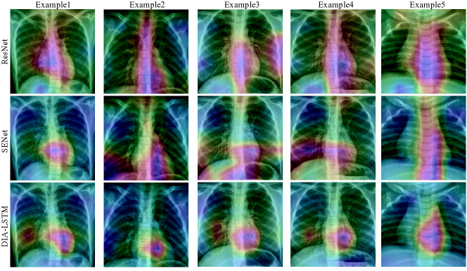
Figure 6: The Grad-CAM visualization for different models. The purple region indicates an essential place for a network to obtain the output, while the dark one is the opposite.

5.2 Object detection

Since the high performance of DIA-LSTM on classification in Section 5.1, in this section, we consider further experiments for object detection tasks on the MS COCO dataset. Specifically, We compare the DIA-LSTM, and DIA-LSTM (Light) with three popular self-attention modules, i.e., SE [9], ECA [23], SGE [32] on the same setting as [35]. We use Faster R-CNN and RetinaNet as detectors, which are implemented by the open-source MMDetection toolkit. The MS COCO dataset contains 80 classes with 118,287 training images and 40,670 test images. The results are shown in Table VIII where all models are verified 15 times with random seeds and the p-value, Average Precision (AP), and other standard COCO metrics are reported.

For the Faster R-CNN detector, We can find that our DIA-LSTM outperforms the baseline models by 2.6% and 2.7% in terms of AP on ResNet50 and ResNet101, respectively. For the RetinaNet detector, the ResNet with DIA-LSTM still surpasses all other models with large margins, and the results of the p-value also reveal that the improvement gained by DIA-LSTM is significant.

5.3 Medical application

In this section, we consider using the proposed DIA-LSTM for a real-world application, i.e., the chest x-ray image classification for pneumonia. We use the dataset from [50], which contains 5,863 X-Ray images and 2 categories (Pneumonia and Normal). The results are shown in Table IX where all models are verified 15 times with random seeds and the mean value and the standard deviations of the classification accuracies are reported. And all models in Table IX are trained from scratch without any pretrain model.

TABLE IX: The results of chest x-ray image classification for pneumonia.

Model	Pneumonia	Normal	All	p-value
ResNet50	97.8	52.5	81.4	*
+SE [9]	99.2	60.8	85.3	*
+DIA-LSTM	99.4	71.1	89.2	N/A
+DIA-LSTM (Light)	99.4	63.7	86.6	*

In Table IX, since the number of the data in each class are imbalanced, we can find that all models can classify the Pneumonia class, but the normal class. Therefore the difficulty of this task is how to correctly distinguish normal x-ray images. The proposed DIA-LSTM can achieve the best performance in this task, and DIA-LSTM (Light) performs the competitive result with respect to SE and has much smaller parameters.

To study the ability of DIA-LSTM in capturing and exploiting features of a given target which is important for the explainable medical application, we apply Grad-CAM [51] to compare the regions where different models localize with respect to their target prediction, which is a well-known tool to generate the heatmap highlighting network attention by the gradient related to the given target. Fig. 6 shows the visualization results and the softmax scores for the target with original ResNet50 and SENet, and DIA-LSTM on the x-ray dataset. The purple region indicates an essential place for a network to obtain the output while the dark one is the opposite.

The results show that DIA-LSTM can extract similar features as SENet, but DIA-LSTM can even capture much more elaborate details of the target, i.e., the region where DIA-LSTM focused on is obviously more concentrated in the lungs, associated with higher confidence for its prediction. Moreover, the original ResNet tends to focus on the region in the middle of the image, i.e., the spine rather than the lungs. These results reveal that the DIA-SLTM may have a more vital ability to emphasize the more discriminative features for normal and pneumonia classes than the original ResNet and SENet.

TABLE X: Test accuracy (%) with different reduction ratio on CIFAR100 with ResNet164. The value in the bracket means the parameter increment compared with the original ResNet164 (1.73M).

Ratio $r$	$\#$P(M)	top1-acc.
1	2.59(+0.86)	77.24
4	1.95(+0.22)	77.09
8	1.84(+0.11)	76.68
16	1.78(+0.05)	76.59

6 Abaltion study

In this section, we conduct ablation experiments to explore how to better plug DIA-LSTM in different neural network structures and gain a deeper understanding of the role of components in the unit. All experiments are performed on CIFAR100 with ResNet. For simplicity, DIANet164 is denoted as a 164-layer ResNet built with DIA-LSTM.

6.1 Reduction Ratio.

The reduction ratio is the only hyper-parameter in DIA-LSTM. The main advantage of our model is improving the versatility of the DNN with a light parameter increment. The smaller reduction ratio causes a higher parameter increment and model complexity. This part investigates the trade-off between model complexity and performance. As shown in Table X, the number of parameters of the DIA-LSTM decreases with the increasing reduction ratio, but the testing accuracy declines slightly, which suggests that the model performance is not sensitive to the reduction ratio. In the case of $r=16$, the ResNet164 with DIA-LSTM has 0.05M parameter increment compared to the original ResNet164 but the testing accuracy of ResNet164 with DIA-LSTM is 76.59% while that of the ResNet164 is 74.32%.

6.2 The Depth of Networks.

Generally, in practice, DNNs with a larger number of parameters do not guarantee sufficient performance improvement. Deeper networks may contain extreme feature and parameter redundancy [34]. Therefore, designing a new structure of deep neural networks is necessary [37, 34, 52, 9, 13, 12]. Since DIA-LSTM affects the topology of DNN backbones, evaluating the effectiveness of DIA-LSTM structure is important. Here we investigate how the depth of DNNs influences DIA-LSTM in two aspects: (1) the performance of DIA-LSTM compared to SENet of various depths; (2) the parameter increment of the ResNet with DIA-LSTM.

TABLE XI: Test accuracy (%) with ResNet of different depth on CIFAR100.

	SENet		DIA-LTSM ($r=4$)
Depth	$\#$P(M)	acc.	$\#$P(M)	acc.
ResNet83	0.99	74.68	1.11(+0.12)	75.72
ResNet164	1.93	75.23	1.95(+0.02)	77.09
ResNet245	2.87	75.43	2.78(-0.09)	77.59
ResNet407	4.74	75.74	4.45(-0.29)	78.08

The results in Table XI show that as the depth increases from 83 to 407 layers, the DIA-LSTM with a smaller number of parameters can achieve higher classification accuracy than the SENet. Moreover, the ResNet83 with DIA-LSTM can achieve a similar performance as the SENet407, and ResNet164 with DIA-LSTM outperforms all the SENets with at least 1.35% and at most 58.8% parameter reduction. They imply that the ResNet with DIA-LSTM is of higher parameter efficiency than SENet. The results also suggest that: as shown in Figure 4, the DIA-LSTM will pass more layers recurrently with a deeper depth. The DIA-LSTM can handle the interrelationship between the information of different layers in much deeper DNN and figure out the long-distance dependency between layers.

6.3 Activation Function and Number of Stacking Cells.

We choose different activation functions in the output layer of DIA-LSTM in Figure 5 (Middle) and different numbers of stacking LSTM cells to explore the effects of these two factors. In Table XII, we find that the performance has been significantly improved after replacing tanh in the standard LSTM with the sigmoid. As shown in Figure 5 (Middle), this activation function is located in the output layer and directly changes the effect of memory unit $c_{t}$ on the output of the output gate. In fact, the sigmoid is used in many attention-based methods like SENet as a gate mechanism. The test accuracy of different choices of LSTM activation functions in Table XII shows that sigmoid better help LSTM as a gate to rescale channel features. Table 12 in the SENet paper [9] shows the performance of different activation functions like sigmoid $>$ tanh $>$ ReLU (bigger is better), which coincides with our reported results and existing observation [33].

When we use sigmoid in the output layer of LSTM, the increasing number of stacking LSTM cells does not necessarily lead to performance improvement but may lead to performance degradation. However, when we choose tanh, the situation is different. It suggests that, through the stacking of LSTM cells, the scale of the information flow among them is changed, which may affect the performance.

TABLE XII: Test accuracy (%) on CIFAR100 with DIANet164 of different activation functions at the output layer in the modified LSTM and the different number of stacking LSTM cells.

$\#$P(M)	Activation	$\#$LSTM cells	top1-acc.
1.95	sigmoid	1	77.09
1.95	tanh	1	75.64
1.95	ReLU	1	75.02
3.33	sigmoid	3	76.07
3.33	tanh	3	76.87

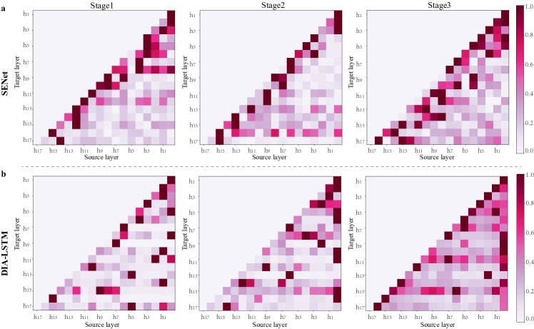
Figure 7: Visualization of feature integration for each stage by random forest. Each row presents the importance of source layers $h_{n},1\leq n<t$ contributing to the target layer $h_{t}$.

7 Analysis

7.1 The effectiveness of the DIA

In this section, we conduct several experiments for DIA-LSTM and analyze how DIA benefits the training from two views: (1) The effect on stabilizing training and (2) the dense-and-implicit connection.

7.1.1 Dense-and-Implicit connection

The view that the dense connections among the different layers can improve the performance is verified in previous work [34]. For the framework in Figure 3, the DIA unit also plays a role in bridging the current layer and the preceding layers such that the DIA unit can adaptively learn the non-linearity relationship between features in two different dimensions. Instead of explicitly dense connections, the DIA unit can implicitly link layers at different depths via a shared module which leads to dense connections.

Specifically, consider a stage consisting of many layers in Figure 8 (Left). It is an explicit structure with a DIA unit, and one layer seems not to connect to the other layers except the network backbone. In fact, the different layers use the parameter-sharing attention module, and the layer-wise information jointly influences the update of learnable parameters in the module, which causes implicit connections between layers with the help of the shared DIA unit as in Figure 8 (Right). Since there is communication between every pair of layers, the connections over all layers are dense.

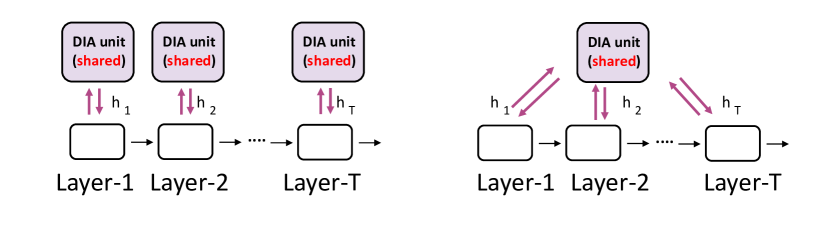
Figure 8: Left. Explicit structure of the network with DIA unit. Right. Implicit connection caused by DIA unit.

TABLE XIII: The test accuracy (%) about the removal of DIA-LSTM unit in different stages.

remove	$\#$P(M)	$\#$P(M)$\downarrow$	top1-acc.	top1-acc.$\downarrow$
stage1	1.94	0.01	76.85	0.24
stage2	1.90	0.05	76.87	0.22
stage3	1.78	0.17	75.78	1.31

TABLE XIV: Testing accuracy (%). We train models of different depths without BN on CIFAR-100. “nan” indicates the numerical explosion.

	Origin		SENet		DIA-LSTM $(r=16)$
Backbone	$\#$P(M)	top1-acc.	$\#$P(M)	top1-acc.	$\#$P(M)	top1-acc.
ResNet83	0.88	nan	0.98	nan	0.94	72.34
ResNet164	1.70	nan	1.91	nan	1.76	73.77
ResNet245	2.53	nan	2.83	nan	2.58	73.86
ResNet326	3.35	nan	3.75	nan	3.41	nan

Next, we can try to further understand the dense connection from the numerical perspective. As shown in Figure 4 and 8, the DIA-LSTM bridges the connections between layers by propagating the information forward through $h_{t}$ and $c_{t}$, leading to feature integration. Moreover, $h_{t}$ at different layers are also integrating with $h_{t^{\prime}},1\leq t^{\prime}<t$ in DIA-LSTM. Notably, $h_{t}$ is applied directly to the features in the network at each layer $t$. Therefore the relationship between $h_{t}$ at different layers somehow reflects the layer-wise connection degree. We explore the nonlinear relationship between the hidden state $h_{t}$ of DIA-LSTM and the preceding hidden state $h_{t-1},h_{t-2},...,h_{1}$, and visualize how the information coming from $h_{t-1},h_{t-2},...,h_{1}$ contributes to $h_{t}$. To reveal this relationship, we consider using the random forest to visualize variable importance. The random forest can return the contributions of input variables to the output separately in the form of importance measure, e.g., Gini importance [53]. The computation details of Gini importance can be referred to the Algorithm 1. For other self-attention modules, like SE, we can also use Algorithm 1 to analyse the relationship between the attention map $h_{t}$ in layer $t$ and the $h_{t-1},h_{t-2},...,h_{1}$ from front layers.

Input: $H$: composed of $h_{1}$,$h_{2}$,…,$h_{t}$ from Stage $i$;

# The size of $H$ is ($b_{z}\times c_{z}\times f_{z}$)

# $b_{z}$ denotes the number of training samples

# $c_{z}$ denotes the number of channels in Stage $i$

# $f_{z}$ denotes the number of layers in Stage $i$

Output: The hotmap $G$ about the feature integration for Stage $i$;

1:initial $G=\emptyset$ ;

2:for $j=1$ to $f_{z}-1$ do

3:     $x\leftarrow[h_{1},h_{2},...,h_{j-1}]$;

4:     $y\leftarrow[h_{j}]$;

5:     $x$ $\leftarrow$ $x$.reshape($b_{z}$,$(f_{z}-j)\times c_{z}$);

6:     RF $\leftarrow$ RandomForestRegressor();

7:     RF.fit($x$,$y$);

8:     Gini_importances $\leftarrow$ RF.feature_importances_; # The length of Gini_importance is $(f_{z}-j)\times c_{z}$

9:     res $\leftarrow$ $\emptyset$; $s$ $\leftarrow$ 0; cnt $\leftarrow$ 0;

10:     for $k=0$ to $(f_{z}-j)$ do

11:         $s$ $\leftarrow$ $s$ + Gini_importance($k$);

12:         cnt $\leftarrow$ cnt + 1;

13:         if cnt == $c_{z}$-1 then

14:              res.add($s$);$s$ $\leftarrow$ 0;cnt $\leftarrow$ 0;

15:         end if$G$.add(res/$\max$(res));

16:     end for

17:end for

Algorithm 1 Calculate feature integration using Gini importance by Random Forest

TABLE XV: Test accuracy (%) of the models without data augment with ResNet164.

Models	CIFAR-10	CIFAR-100
ResNet164	87.16	61.42
SENet	87.21	63.92
DIANet	89.42	67.86

Take $h_{n},1\leq n<t$ as input variables and $h_{t}$ as output variable, we can get the Gini importance of each variable $h_{n},1\leq n<t$. ResNet164 contains three stages, and each stage consists of 18 layers. We conduct three Gini importance computations for each stage separately. As shown in Figure 7, each row presents the importance of source layers $h_{n},1\leq n<t$ contributing to the target layer $h_{t}$. In each sub-graph of Figure 7, the diversity of variable importance distribution indicates that the current layer uses the information of the preceding layers. The interaction between shallow and deep layers in the same stage reveals the effect of implicitly dense connection. In particular, for the results of DIA-LSTM, taking $h_{17}$ in stage 1 (the last row) as an example, $h_{16}$ or $h_{15}$ does not intuitively provide the most information for $h_{17}$, but $h_{5}$ does. The DIA unit can adaptively integrate information between multiple layers. Unlike the DIA-LSTM, the information in each layer of the SENet tends to be strongly correlated with the information in the previous one or two layers, i.e., the Gini importance in the diagonal is significantly larger than that in the other positions. Moreover, in Figure 7 (stage 3) for DIA-LSTM, the information interaction with previous layers in stage 3 is more intense and frequent than that of the first two stages. Correspondingly, as shown in Table XIII, in the experiments when we remove the DIA-LSTM unit in stage 3, the classification accuracy decreases from 77.09 to 76.85. However, when it is removed in stage 1 or 2, the performance degradation is very similar, falling to 76.85 and 76.87 respectively. Also note that for DIANet, the number of parameter increments in stage 2 is larger than that of stage 1. It implies that the significant performance degradation after the removal of stage 3 may be not only due to the reduction of the number of parameters but due to the lack of dense feature integration.

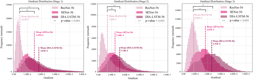
Figure 9: The distribution of gradient in each stage of ResNet56 without all the skip connections.

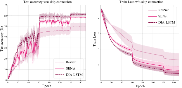
Figure 10: The test accuracy and train loss of ResNet164 without skip connection.

7.1.2 The Effect on Stabilizing Training

In Section 7.1.1, we reveal that the existing of dense-and-implicit connections. In this section, we conduct several experiments to demonstrate the regularization effect of these connections on stabilizing training.

Removal of Batch Normalization. Small changes in shallower hidden layers may be amplified as the information propagates within the deep architecture and sometimes result in a numerical explosion. Batch Normalization (BN) [54] is widely used in deep networks since it stabilizes the training by normalization the input of each layer. DIA-LSTM unit recalibrates the feature maps by channel-wise multiplication, which plays a role of scaling similar to BN. Table XIV shows the performance of the models of different depths trained on CIFAR100 and BNs are removed in these networks. The experiments are conducted on a single GPU with a batch size of 128 and an initial learning rate of 0.1. Both the original ResNet and SENet face the problem of numerical explosion without BN while the DIA-LSTM can be trained with depth up to 245. In Table XIV, at the same depth, SENet has a larger number of parameters than DIA-LSTM but still comes to numerical explosion without BN, which means that the number of parameters is not the case for stabilization of training, but sharing mechanism we proposed may be the case. Besides, compared with Table XI, the testing accuracy of DIA-LSTM without BN still can keep up to 70%. The scaling learned by DIA-LSTM integrates the information from preceding layers and enables the network to choose a better scaling for features of the current layer.

Without Data Augmentation. Explicit dense connections may help bring more efficient usage of parameters, which makes the neural network less prone to overfit [34]. Although the dense connections in DIA-LSTM are implicit, our method still shows the ability to reduce overfitting. To verify it, We train the models without data augment to reduce the influence of regularization from data augment. As shown in Table XV, ResNet164 with DIA-LSMT achieves lower testing errors than the original ResNet164 and SENet. To some extent, the implicit and dense structure of our method may have a regularization effect.

Removal of Skip Connection. The skip connection has become a necessary structure for training DNNs [55]. Without skip connection, the DNN is hard to train due to the reasons like the gradient vanishing [56, 57, 52]. We conduct the experiment where all the skip connections are removed in ResNet56 and count the absolute value of the gradient at the output tensor of each stage. As shown in Figure 9 which presents the gradient distribution with all skip connection removal, the ResNet56 with DIA-LSTM obviously enlarges the mean and variance of the gradient distribution, which enables larger absolute value and diversity of gradient and relieves gradient degradation to some extent.

Further, we can explore the effectiveness of DIA-LSTM from the perspective of test accuracy and train loss while the model is trained without skip connection. Specifically, we follow the training setting in [44] to train the ResNet with different self-attention modules, which is shown in Figure 10. For test accuracy, we can find that the skip connection plays a big role in the training. When the skip connection is not used, the performance of the model decreases greatly, and the classification accuracy of all models drops to between 50% and 65%. Moreover, all test accuracy curves look oscillating, which means that the training of the model becomes unstable without skip connections. For this case, DIA-LSTM can significantly mitigate the performance loss due to not using skip connections compared to the original ResNet and SENet. Similarly, for train loss, DIA-LSTM still achieves the fastest loss degradation. These two experiments imply that DIA-LSTM can be a good regularizer for the training of neural networks.

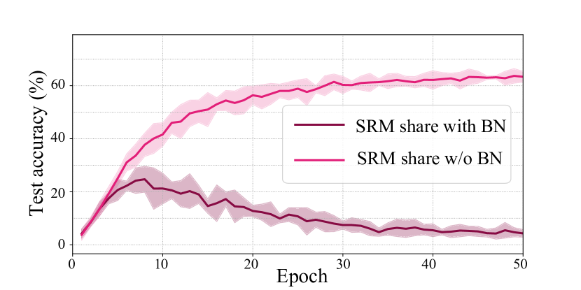
Figure 11: The performance of SRM with two sharing strategies.

7.2 Number of Parameters in LSTM

This section shows the number of parameter costs in the standard LSTM and the modified LSTM in Figure 5 with the reduction ratio $r$. The input $y_{t}$, the hidden state vector $h_{t-1}$ and the output in Figure 5 are of the same size $N$, which is equal to the number of channels.

Standard LSTM. There are four linear transformations in the standard LSTM as shown in Figure 5 (Left) to control the information flow with input $y_{t}$ and $h_{t-1}$ respectively. To simplify the calculation, the bias is omitted. Therefore, for the $y_{t}$, the number of parameters of four linear transformations equals $4N^{2}$. Similarly, the number parameters of four linear transformations for input $h_{t-1}$ is equal to $4N^{2}$. The total number equals $8N^{2}.$

DIA-LSTM. As shown in Figure 5 (Middle), there is a linear transformation to reduce the dimension at the beginning, which reduces the dimension of input $y_{t}$ from $N$ to $N/r$. The number of parameters for the linear transformation is equal to $N^{2}/r$. Then the output will be passed to four linear transformations the same as the standard LSTM. The number of parameters of four linear transformations is equal to $4N^{2}/r$. Therefore, for input $y_{t}$ and reduction ratio $r$, the total number of parameters is $5N^{2}/r$. Similarly, the number of parameters with input $h_{t-1}$ is the same as that concerning the input $y_{t}$. The total number of parameters is $10N^{2}/r.$ In Figure 5 (Right), the DIA-LSTM (Light) use “IE” in Eq.5 to replace several linear transformations in Figure 5 (Middle), leading to smaller number of parameters and faster inference speed.

7.3 Discussion

In this section, we have the discussion for DIA-LSTM, i.e., the computational cost and the sharing strategy.

7.3.1 Computational cost

As shown in our comprehensive experiments in Section 5, the use of LSTM is greatly beneficial for our proposed framework. However, the use of LSTM may increase the computational cost and training time. Taking ResNet164 as an example, the inference of ResNet164 with standard DIA-LSTM is about 12% slower than that without any self-attention module. Therefore, when DIA-LSTM needs to be applied to some applications that are sensitive to computational speed, the more efficient LSTM design, like Figure 5 can mitigate this issue with some performance loss. Specifically, DIA-LSTM (Light) can reduce this bottleneck of computational cost from 12% to only 1%.

7.3.2 DIA with batch normalization

Although the proposed framework, i.e., Figure 3, can boost many existing self-attention modules, not all of them can be shared directly throughout the layer of the backbone. As highlighted in Table III, when SRM is applied to the DIA unit, the batch normalization (BN) is not shared in the unit due to some of its properties. Specifically, BN is a common component in deep learning that is used in the design of many neural network structures, and likewise contains self-attention mechanism design [srm,iebn]. However, some previous works [share] have revealed that the statistics calculated by BN are closely related to the characteristics of the layer where it is located. For some tasks, these statistics are not encouraged to be used across layers. Therefore, when we apply the framework shown in Figure 3 to a given self-attention module, BN should not be shared throughout the layer, and each block should be set to its own BN. Figure 11 shows the classification results of the first 50 epochs for two different sharing strategies of the SRM module. We can find that if BN is shared, then the classification performance of the model goes up and down early in training, and drops rapidly to an accuracy close to 0. If BN does not participate in sharing, the classification accuracy of the model normally increases, which is consistent with our analysis.

8 Conclusion

In this paper, inspired by the dynamical system perspective of ResNet, we propose a novel-and-simple framework that shares an attention module throughout different network layers to encourage the integration of layer-wise information. The parameter-sharing module is called the dense-and-implicit attention (DIA) unit. We propose incorporating LSTM in DIA unit (DIA-LSTM) and show the effectiveness of DIA-LSTM for several popular vision tasks by conducting experiments on benchmark datasets and popular networks. We further empirically show that the the dense and implicit connections formed by our method has a strong regularization ability to stabilize the training of deep networks by the experiments with the removal of skip connections, data augmentation, batch normalization in the whole residual network.

References

- [1] J. R. Anderson, Cognitive psychology and its implications. Macmillan, 2005.
- [2] J. Xie, Z. Ma, D. Chang, G. Zhang, and J. Guo, “Gpca: A probabilistic framework for gaussian process embedded channel attention,” IEEE Transactions on Pattern Analysis and Machine Intelligence, 2021.
- [3] A. Vaswani, N. Shazeer, N. Parmar, J. Uszkoreit, L. Jones, A. N. Gomez, Ł. Kaiser, and I. Polosukhin, “Attention is all you need,” in Advances in neural information processing systems, 2017, pp. 5998–6008.
- [4] D. Britz, A. Goldie, M.-T. Luong, and Q. Le, “Massive exploration of neural machine translation architectures,” arXiv preprint arXiv:1703.03906, 2017.
- [5] J. Cheng, L. Dong, and M. Lapata, “Long short-term memory-networks for machine reading,” EMNLP 2016, 2016.
- [6] K. Xu, J. L. Ba, R. Kiros, K. Cho, A. Courville, R. Salakhutdinov, R. S. Zemel, and Y. Bengio, “Show, attend and tell: Neural image caption generation with visual attention,” in Proceedings of the 32Nd International Conference on International Conference on Machine Learning - Volume 37, ser. ICML’15. JMLR.org, 2015, pp. 2048–2057. [Online]. Available: http://dl.acm.org/citation.cfm?id=3045118.3045336
- [7] M.-T. Luong, H. Pham, and C. D. Manning, “Effective approaches to attention-based neural machine translation,” arXiv preprint arXiv:1508.04025, 2015.
- [8] A. Miech, I. Laptev, and J. Sivic, “Learnable pooling with context gating for video classification,” arXiv preprint arXiv:1706.06905, 2017.
- [9] J. Hu, L. Shen, and G. Sun, “Squeeze-and-excitation networks,” in Proceedings of the IEEE conference on computer vision and pattern recognition, 2018, pp. 7132–7141.
- [10] S. Woo, J. Park, J.-Y. Lee, and I. So Kweon, “Cbam: Convolutional block attention module,” in Proceedings of the European Conference on Computer Vision (ECCV), 2018, pp. 3–19.
- [11] J. Park, S. Woo, J.-Y. Lee, and I. S. Kweon, “Bam: Bottleneck attention module,” arXiv preprint arXiv:1807.06514, 2018.
- [12] X. Wang, R. Girshick, A. Gupta, and K. He, “Non-local neural networks,” in Proceedings of the IEEE Conference on Computer Vision and Pattern Recognition, 2018, pp. 7794–7803.
- [13] J. Hu, L. Shen, S. Albanie, G. Sun, and A. Vedaldi, “Gather-excite: Exploiting feature context in convolutional neural networks,” in Advances in Neural Information Processing Systems, 2018, pp. 9401–9411.
- [14] Y. Cao, J. Xu, S. Lin, F. Wei, and H. Hu, “Gcnet: Non-local networks meet squeeze-excitation networks and beyond,” arXiv preprint arXiv:1904.11492, 2019.
- [15] X. Li, W. Wang, X. Hu, and J. Yang, “Selective kernel networks,” in Proceedings of the IEEE Conference on Computer Vision and Pattern Recognition, 2019, pp. 510–519.
- [16] J. Wang, Y. Chen, S. X. Yu, B. Cheung, and Y. LeCun, “Recurrent parameter generators,” arXiv preprint arXiv:2107.07110, 2021.
- [17] F. Stelzer, A. Röhm, R. Vicente, I. Fischer, and S. Yanchuk, “Deep neural networks using a single neuron: folded-in-time architecture using feedback-modulated delay loops,” Nature communications, vol. 12, no. 1, pp. 1–10, 2021.
- [18] S. Jaiswal, B. Fernando, and C. Tan, “Tdam: Top-down attention module for contextually guided feature selection in cnns,” 2021.
- [19] Z. Shen, Z. Liu, and E. Xing, “Sliced recursive transformer,” arXiv preprint arXiv:2111.05297, 2021.
- [20] J. Zhang, H. Peng, K. Wu, M. Liu, B. Xiao, J. Fu, and L. Yuan, “Minivit: Compressing vision transformers with weight multiplexing,” in Proceedings of the IEEE/CVF Conference on Computer Vision and Pattern Recognition, 2022, pp. 12 145–12 154.
- [21] V. Sze, Y.-H. Chen, T.-J. Yang, and J. S. Emer, “Efficient processing of deep neural networks: A tutorial and survey,” Proceedings of the IEEE, vol. 105, no. 12, pp. 2295–2329, 2017.
- [22] Y. Hua, L. Mou, and X. X. Zhu, “Lahnet: A convolutional neural network fusing low-and high-level features for aerial scene classification,” in IGARSS 2018-2018 IEEE International Geoscience and Remote Sensing Symposium. IEEE, 2018, pp. 4728–4731.
- [23] Q. Wang, B. Wu, P. Zhu, P. Li, W. Zuo, and Q. Hu, “Eca-net: Efficient channel attention for deep convolutional neural networks,” in The IEEE Conference on Computer Vision and Pattern Recognition (CVPR), 2020.
- [24] H. Lee, H.-E. Kim, and H. Nam, “Srm: A style-based recalibration module for convolutional neural networks,” in Proceedings of the IEEE/CVF International Conference on Computer Vision, 2019, pp. 1854–1862.
- [25] J. Guo, X. Ma, A. Sansom, M. McGuire, A. Kalaani, Q. Chen, S. Tang, Q. Yang, and S. Fu, “Spanet: Spatial pyramid attention network for enhanced image recognition,” in 2020 IEEE International Conference on Multimedia and Expo (ICME). IEEE, 2020, pp. 1–6.
- [26] V. Mnih, N. Heess, A. Graves et al., “Recurrent models of visual attention,” in Advances in neural information processing systems, 2014, pp. 2204–2212.
- [27] B. Zhao, X. Wu, J. Feng, Q. Peng, and S. Yan, “Diversified visual attention networks for fine-grained object classification,” IEEE Transactions on Multimedia, vol. 19, no. 6, pp. 1245–1256, 2017.
- [28] Z. Huang, S. Liang, M. Liang, W. He, H. Yang, and L. Lin, “The lottery ticket hypothesis for self-attention in convolutional neural network,” arXiv preprint arXiv:2207.07858, 2022.
- [29] Z. Huang, S. Liang, M. Liang, W. He, and H. Yang, “Efficient attention network: Accelerate attention by searching where to plug,” arXiv preprint arXiv:2011.14058, 2020.
- [30] X. Wang, Z. Cai, D. Gao, and N. Vasconcelos, “Towards universal object detection by domain attention,” CoRR, vol. abs/1904.04402. [Online]. Available: http://arxiv.org/abs/1904.04402
- [31] F. Wang, M. Jiang, C. Qian, S. Yang, C. Li, H. Zhang, X. Wang, and X. Tang, “Residual attention network for image classification,” in The IEEE Conference on Computer Vision and Pattern Recognition (CVPR), July 2017.
- [32] X. Li, X. Hu, and J. Yang, “Spatial group-wise enhance: Improving semantic feature learning in convolutional networks,” arXiv preprint arXiv:1905.09646, 2019.
- [33] S. Liang, Z. Huang, M. Liang, and H. Yang, “Instance enhancement batch normalization: An adaptive regulator of batch noise,” in Proceedings of the AAAI Conference on Artificial Intelligence, vol. 34, no. 04, 2020, pp. 4819–4827.
- [34] G. Huang, Z. Liu, K. Q. Weinberger, and L. van der Maaten, “Densely connected convolutional networks,” in Computer Vision and Pattern Recognition, 2017.
- [35] J. Zhao, Y. Fang, and G. Li, “Recurrence along depth: Deep convolutional neural networks with recurrent layer aggregation,” Advances in Neural Information Processing Systems, vol. 34, pp. 10 627–10 640, 2021.
- [36] M. Lin, Q. Chen, and S. Yan, “Network in network,” arXiv preprint arXiv:1312.4400, 2013.
- [37] K. He, X. Zhang, S. Ren, and J. Sun, “Deep residual learning for image recognition,” in Computer Vision and Pattern Recognition, 2016.
- [38] R. K. Srivastava, K. Greff, and J. Schmidhuber, “Highway networks,” arXiv preprint arXiv:1505.00387, 2015.
- [39] L. Wolf and S. Bileschi, “A critical view of context,” International Journal of Computer Vision, vol. 69, no. 2, pp. 251–261, 2006.
- [40] H. Li, W. Ouyang, and X. Wang, “Multi-bias non-linear activation in deep neural networks,” in International conference on machine learning, 2016, pp. 221–229.
- [41] S. Hochreiter and J. Schmidhuber, “Long short-term memory,” Neural computation, vol. 9, no. 8, pp. 1735–1780, 1997.
- [42] S. Zhong, W. Wen, and J. Qin, “Switchable self-attention module,” arXiv preprint arXiv:2209.05680, 2022.
- [43] S. Zhong and W. Wen, “Mix-pooling strategy for attention mechanism,” arXiv preprint arXiv:2208.10322, 2022.
- [44] Z. Huang, S. Liang, M. Liang, and H. Yang, “Dianet: Dense-and-implicit attention network.” in AAAI, 2020, pp. 4206–4214.
- [45] A. Krizhevsky, G. Hinton et al., “Learning multiple layers of features from tiny images,” 2009.
- [46] A. Coates, A. Ng, and H. Lee, “An analysis of single-layer networks in unsupervised feature learning,” in Proceedings of the Fourteenth International Conference on Artificial Intelligence and Statistics, ser. Proceedings of Machine Learning Research, G. Gordon, D. Dunson, and M. Dudík, Eds., vol. 15. Fort Lauderdale, FL, USA: PMLR, 11–13 Apr 2011, pp. 215–223.
- [47] O. Vinyals, C. Blundell, T. Lillicrap, k. kavukcuoglu, and D. Wierstra, “Matching networks for one shot learning,” in Advances in Neural Information Processing Systems, D. Lee, M. Sugiyama, U. Luxburg, I. Guyon, and R. Garnett, Eds., vol. 29. Curran Associates, Inc., 2016. [Online]. Available: https://proceedings.neurips.cc/paper/2016/file/90e1357833654983612fb05e3ec9148c-Paper.pdf
- [48] S. Zagoruyko and N. Komodakis, “Wide residual networks,” in BMVC, 2016.
- [49] S. Xie, R. Girshick, P. Dollár, Z. Tu, and K. He, “Aggregated residual transformations for deep neural networks,” in Proceedings of the IEEE conference on computer vision and pattern recognition, 2017, pp. 1492–1500.
- [50] D. S. Kermany, M. Goldbaum, W. Cai, C. C. Valentim, H. Liang, S. L. Baxter, A. McKeown, G. Yang, X. Wu, F. Yan et al., “Identifying medical diagnoses and treatable diseases by image-based deep learning,” Cell, vol. 172, no. 5, pp. 1122–1131, 2018.
- [51] R. R. Selvaraju, M. Cogswell, A. Das, R. Vedantam, D. Parikh, and D. Batra, “Grad-cam: Visual explanations from deep networks via gradient-based localization,” in Proceedings of the IEEE international conference on computer vision, 2017, pp. 618–626.
- [52] R. K. Srivastava, K. Greff, and J. Schmidhuber, “Training very deep networks,” in Advances in neural information processing systems, 2015, pp. 2377–2385.
- [53] B. Gregorutti, B. Michel, and P. Saint-Pierre, “Correlation and variable importance in random forests,” Statistics Computing, vol. 27, no. 3, pp. 659–678, 2017.
- [54] S. Ioffe and C. Szegedy, “Batch normalization: Accelerating deep network training by reducing internal covariate shift,” in Proceedings of the 32Nd International Conference on International Conference on Machine Learning - Volume 37, ser. ICML’15. JMLR.org, 2015, pp. 448–456. [Online]. Available: http://dl.acm.org/citation.cfm?id=3045118.3045167
- [55] K. He, X. Zhang, S. Ren, and J. Sun, “Identity mappings in deep residual networks,” in European Conference on Computer Vision, 2016.
- [56] Y. Bengio, P. Simard, P. Frasconi et al., “Learning long-term dependencies with gradient descent is difficult,” IEEE transactions on neural networks, vol. 5, no. 2, pp. 157–166, 1994.
- [57] X. Glorot and Y. Bengio, “Understanding the difficulty of training deep feedforward neural networks,” in Proceedings of the thirteenth international conference on artificial intelligence and statistics, 2010, pp. 249–256.