An Empirical Evaluation of Zeroth-Order Optimization Methods on AI-driven Molecule Optimization

Abstract

Molecule optimization is an important problem in chemical discovery and has been approached using many techniques, including generative modeling, reinforcement learning, genetic algorithms, and much more. Recent work has also applied zeroth-order (ZO) optimization, a subset of gradient-free optimization that solves problems similarly to gradient-based methods, for optimizing latent vector representations from an autoencoder. In this paper, we study the effectiveness of various ZO optimization methods for optimizing molecular objectives, which are characterized by variable smoothness, infrequent optima, and other challenges. We provide insights on the robustness of various ZO optimizers in this setting, show the advantages of ZO sign-based gradient descent (ZO-signGD), discuss how ZO optimization can be used practically in realistic discovery tasks, and demonstrate the potential effectiveness of ZO optimization methods on widely used benchmark tasks from the Guacamol suite. Code is available at: https://github.com/IBM/QMO-bench.

1 Introduction

The goal of molecule optimization is to efficiently find molecules possessing desirable chemical properties. As the ability to effectively solve difficult molecule optimization tasks would greatly accelerate the discovery of promising drug candidates and decrease the immense resources necessary for drug development, significant efforts have been dedicated to designing molecule optimization algorithms leveraging a variety of techniques, including deep reinforcement learning [1], genetic algorithms [2], Bayesian optimization [3], variational autoencoders [4, 5], and more. Several molecule optimization benchmark tasks have also been proposed, including similarity-based oracles [6] and docking scores [7].

In this paper, we extend the work of Hoffman et al. [8], who proposed the use of ZO optimization in their query-based molecule optimization (QMO) framework, an end-to-end framework which decouples molecule representation learning and property prediction. QMO iteratively optimizes a starting molecule, making it well suited for lead optimization tasks, but it can also start from random points and traverse large distances to find optimal molecules. In comparison with the work of Hoffman et al. [8] which experiments with only one optimizer, we experiment with variations of QMO using different ZO optimizers. Furthermore, we add more benchmark tasks from Guacamol [6] (whose use has been encouraged by the molecule optimization community [3, 9] and used by Gao et al. [10] to benchmark many design algorithms in a standardized setting), and provide insights into the challenges of ZO optimization on molecular objectives.

Contributions

We evaluate several ZO optimization methods for the problem of molecule optimization in terms of convergence speed, convergence accuracy, and robustness to the unusual function landscapes (described further in Section 2.4) of molecular objectives. We show that ZO-signGD [11] outperforms other methods for molecule optimization in not only speed but also accuracy, despite being known to have worse convergence accuracy for other problems like adversarial attacks [11], which indicates that the sign operation is potentially more robust to the function landscapes of molecular objectives. Furthermore, we provide insights into practical application of ZO optimization in drug discovery scenarios for both lead optimization tasks and the discovery of novel molecules, as well as propose the use of a hybrid approach combining others models with QMO.

Related work

ZO optimization is a class of methods used for solving black-box problems by estimating gradients using only zeroth-order function evaluations and performing iterative updates as in first-order methods like gradient descent (GD) [12]. Many types of ZO optimization algorithms have been developed, including ZO gradient descent (ZO-GD) [13], ZO-signGD [11], ZO adaptive momentum method (ZO-AdaMM, or ZO-Adam specifically for the Adam variant) [14], and more [15, 16]. The optimality of ZO optimization methods has also been studied under given problem assumptions [17]. ZO optimization methods have achieved impressive feats in adversarial machine learning, where they have been used for adversarial example generation in black-box settings and demonstrated comparable success to first-order white-box attacks [18, 19]. They have also been shown to be able to generate contrastive explanations for black-box models [20]. Finally, Hoffman et al. [8] showed how ZO optimization methods can also be applied to molecule optimization with their QMO framework.

2 QMO: Background and Variations

2.1 QMO framework

Following the QMO framework by Hoffman et al. [8], we use an autoencoder to encode molecules with encoder $E:\mathcal{X}\mapsto\mathbb{R}^{d}$ and decode latent vectors with decoder $D:\mathbb{R}^{d}\mapsto\mathcal{X}$, where $\mathcal{X}$ denotes the discrete chemical space of all drug candidates. We denote with $\mathcal{O}:\mathcal{X}\mapsto\mathbb{R}$ a black-box oracle returning a scalar corresponding to a molecular property of interest (which may also be modified by adding losses related to other properties), and for ease of notation with the QMO framework, we define our optimization objective loss function as $f(\mathbf{z})=-\mathcal{O}(D(\mathbf{z}))$ for latent representations $\mathbf{z}\in\mathbb{R}^{d}$. As each function query $f(\mathbf{z})$ queries the oracle $\mathcal{O}$ with the decoded molecule corresponding to $\mathbf{z}$, one function query is equivalent to one oracle query.

In QMO, we use ZO optimization methods to navigate the latent space to solve $\mathrm{min}_{\mathbf{z}}f(\mathbf{z})$. Specifically, given a starting molecule and its latent representation $\mathbf{z}_{0}$, we iteratively update the current latent representation following some optimizer, as done in first-order gradient-based methods like gradient descent. But as we do not have any first-order oracle, we instead use gradients estimated using only evaluations of $f$ following some gradient estimator. The QMO framework, which closely follows a generic ZO optimization procedure, is summarized in Algorithm 1.

Algorithm 1 Generic QMO framework for molecule optimization

1:Inputs: Starting molecule $x_{0}\in\mathcal{X}$, encoder $E$, decoder $D$, gradient estimation operation $\mathrm{estimate\_{gradient}}_{f}(\cdot)$ for function $f$, optimizer updating operation $\mathrm{update}(\cdot)$, number of iterations $T$, and learning rate $\alpha$

2:$\mathcal{Z}_{\mathrm{iterate}}\leftarrow\{\emptyset\}$

3:$\mathbf{z}_{0}\leftarrow E(x_{0})$

4:for $t=0,1,...,T-1$ do

5:     $\hat{\mathbf{g}}_{t}\leftarrow\mathrm{estimate\_{gradient}}_{f}(\mathbf{z}_{t},E,D)$

6:     $\mathbf{z}_{t+1}\leftarrow\mathrm{update}(\mathbf{z}_{t},\{\hat{\mathbf{g}}_{i}\}_{i=1}^{t},\alpha,E,D)$

7:     $\mathcal{Z}_{\mathrm{iterate}}\leftarrow\mathcal{Z}_{\mathrm{iterate}}\cup\{\mathbf{z}_{t+1}\}$

8:end for

In principle, QMO is a generic framework which can guide searches over any continuous learned representation based on any discrete space and use any ZO optimization method. Hoffman et al. [8] used the pre-trained SMILES-based [21] autoencoder (CDDD model) from Winter et al. [22] with embedding dimension $d=512$ and ZO-Adam. Here, we use the same autoencoder but consider several variations of QMO using different gradient estimators and optimizers to provide a comprehensive study on the effect of ZO optimization methods.

As a note, QMO is applicable to molecule optimization with design constraints. For example, given a set of property scores $\{p_{i}\}_{i=1}^{I}$ to be optimized with positive coefficients $\{\gamma_{i}\}_{i=1}^{I}$ and a set of property constraints $\{c_{j}\}_{j=1}^{J}$ with thresholds $\{\eta_{j}\}_{j=1}^{J}$, we can define the oracle as

$$\mathcal{O}(x)=\sum_{i=1}^{I}\gamma_{i}\cdot p_{i}(x)-\sum_{j=1}^{J}\mathrm{max}(\eta_{j}-c_{j}(x),0)$$ (1)

where $x\in\mathcal{X}$. The vectors $\mathbf{z}\in\mathcal{Z}_{\mathrm{iterate}}$ not satisfying $c_{j}(D(\mathbf{z}))\geq\eta_{j}$ for all $j\in\{1,2,...,J\}$ can then be removed from $\mathcal{Z}_{\mathrm{iterate}}$.

2.2 ZO gradient estimators

We consider two main ZO gradient estimators. Both average finite differences over $Q$ independently sampled random perturbations $\{\mathbf{u}_{q}\}_{q=1}^{Q}$, include a smoothing parameter $\beta$, and follow the form:

$$\widehat{\nabla}f(\mathbf{z})=\frac{\varphi(d)}{\beta\cdot Q}\sum_{q=1}^{Q}{[f(\mathbf{z}+\beta\mathbf{u}_{q})-f(\mathbf{z})]\mathbf{u}_{q}}$$ (2)

The two gradient estimators differ mainly on the sampling method for each random direction $\mathbf{u}_{q}$, and also by the dimension-dependent factor $\varphi(d)$. They are:

• Gaussian smoothing (GS) [13, 23]: when we sample each direction from the uniform distribution $\mathcal{U}(\mathcal{S}(0,1))$ on the unit sphere. For GS, $\varphi(d)=d$.

• Bernoulli smoothing-shrinkage (BeS-shrink) [24]: when we craft each random direction by independently sampling each of its $d$ entries from $(B_{0.5}-0.5)/m$, where $B_{0.5}$ follows the Bernoulli distribution with probability $0.5$ and $m=\sqrt{\nicefrac{{Q+d-1}}{{4Q}}}$ is an optimal shrinking factor. For BeS-shrink, $\varphi(d)=1$.

By averaging over $Q$ random directions to decrease estimation error, the gradient estimation operation requires querying $Q+1$ different points (which are each decoded into a molecule and used to query oracle $\mathcal{O}$). We therefore require $Q+1$ oracle evaluations for each optimization iteration.

Additionally, because the above gradient estimators use a (forward) finite difference of 2 points to estimate the gradient for each random perturbation, we refer to it as a 2-point gradient estimator. An alternative to the 2-point GS and BeS-shrink gradient estimators are their 1-point alternatives, which instead have the form:

$$\widehat{\nabla}f(\mathbf{z})=\frac{\varphi(d)}{\beta\cdot Q}\sum_{q=1}^{Q}{f(\mathbf{z}+\beta\mathbf{u}_{q})\mathbf{u}_{q}}$$ (3)

Similar to 2-point gradient estimators, 1-point estimators require $Q+1$ oracle queries at each iteration (the estimation operation itself requires only $Q$ queries, but this does not account for querying the updated molecule after each iteration). However, 1-point estimators are not commonly used in practice due to higher variance.

2.3 ZO optimizers

We consider three main optimizers, each having its own updating operation that consists of computing a descent direction $\mathbf{m}_{t}$ and then updating the current point. Each optimizer can be paired with any ZO gradient estimator. The three are as follows:

• ZO gradient descent (ZO-GD) [13]: analogous to stochastic gradient descent (SGD) in the first-order stochastic setting. ZO-GD uses the current gradient estimate as the descent direction $\mathbf{m}_{t}=\hat{\mathbf{g}}_{t}$ and updates the current point via the rule $\mathbf{z}_{t+1}=\mathbf{z}_{t}-\alpha\mathbf{m}_{t}$.

• ZO sign-based gradient descent (ZO-signGD) [11]: analogous to sign-based SGD (signSGD) [25] in the first-order stochastic setting. ZO-signGD uses the same point updating rule as ZO-GD but instead uses the sign of the current estimate as the descent direction $\mathbf{m}_{t}=\mathrm{sign}(\hat{\mathbf{g}}_{t})$, where $\mathrm{sign}(\cdot)$ denotes the element-wise sign operation.

• ZO-Adam [14]: analogous to Adam [26] in the first-order stochastic setting. ZO-Adam adopts a momentum-type descent direction and an adaptive learning rate.

Table 1: Summary of ZO optimization methods considered.

ZO optimization method	Gradient estimator	Optimizer
Adam-2p-BeS-shrink	2-point BeS-shrink	Adam
Adam-2p-GS	2-point GS	Adam
GD-2p-BeS-shrink	2-point BeS-shrink	GD
GD-2p-GS	2-point GS	GD
signGD-2p-BeS-shrink	2-point BeS-shrink	signGD
signGD-2p-GS	2-point GS	signGD

The ZO optimization methods compared in this paper are summarized in Table 1.

2.4 Motivating the comparison of ZO optimization methods for molecule optimization

We motivate our comparison of optimizers not only in terms of convergence speed and convergence accuracy, but also in terms of robustness to the unfriendly function landscapes of molecular objectives. Indeed, molecule optimization is made difficult by variable function smoothness due to "activity cliffs" in the molecular space where small structural changes cause large changes in oracle values [9]. As optima are infrequent, there are also large and extremely "flat" unfavorable regions in the space, where the oracle values change minimally and may be very small. Furthermore, because our objective function $f$ obtains values by querying the oracle $\mathcal{O}$ using discrete molecular representations obtained from decoding the latent vectors, the function landscape is made discrete and thus further non-smooth (i.e., the function value may have a discrete "jump" at the borders between adjacent regions of latent vectors which decode to different molecules, see Fig. 1). Thus, being able to effectively navigate the latent chemical space and not get stuck in unfavorable regions is an important and non-trivial attribute to pursue in optimization methods.

Sign-based gradient descent is known to be effective in achieving fast convergence speed in stochastic settings: in the stochastic first-order oracle setting, Bernstein et al. [25] showed that signSGD could have faster empirical convergence speed than SGD, and in the zeroth-order stochastic setting Liu et al. [11] similarly showed that ZO-signSGD has faster convergence speed than many ZO optimization methods at the cost of worse accuracy (i.e., converging only to the neighborhood of an optima). The fast convergence of sign-based methods is motivated by the idea that the sign operation is more robust to stochastic noise, and though our formulation of molecule optimization is non-stochastic, the sign operation is potentially more robust to the difficult landscapes of molecular objective functions. Adaptive momentum methods like Adam also make use of the sign of stochastic gradients for determining the descent direction in addition to variance adaption [27], and thus ZO-Adam may also show robustness to the function landscape.

3 Practical Usage of QMO for Drug Discovery

We imagine QMO can be applied for two main cases: 1) identifying novel lead molecules (finding molecules significantly different from known leads), and 2) lead optimization (finding slightly modified versions of known leads).

For the former application case, it may be counterproductive to use known leads as the starting molecule in QMO, as those leads may be in the close neighborhood of a local optima (or a local optima themselves) in the function landscape, in which the optimizer would likely get stuck (preventing the exploration of different areas of the latent chemical space). Instead, it may be more promising to start at a random point in the chemical space. QMO also has the advantage that it guides search without the use of a training set, which aids in finding candidates vastly different from known molecules. However, finding a highly diverse set of novel leads may be unlikely within a single run of QMO as the optimization methods converge to some neighborhood, meaning that multiple random restarts would likely be necessary to discover a diverse set of lead molecules.

For the latter application case, it is much more sensible to use known leads as the starting molecule input to QMO. Additionally, rather than using an oracle $\mathcal{O}$ evaluating only the main desired drug property (i.e., activity against a biological target), it may be advantageous to use a modified oracle. For example, Hoffman et al. [8] apply QMO for lead optimization of known SARS-CoV-2 main protease inhibitors and antimicrobial peptides (AMPs) following the constrained molecule optimization setting of (1), with pre-trained property predictors for each task. They set similarity to the original lead molecule as the property score $p_{\mathrm{sim}}$ to be optimized, and set constraints on properties of interest (binding affinity $c_{\mathrm{aff}}$ for the SARS-CoV-2 task, or toxicity prediction value $c_{\mathrm{tox}}$ and AMP prediction value $c_{\mathrm{AMP}}$ for the AMP task). In these formulations, the main optimization objective is actually molecular similarity rather than the main properties of interest.

Hybrid optimization: Integrating QMO with generative models

Additionally, in this paper we propose to integrate QMO with other models in a hybrid approach: namely, we can use molecules generated by other models as input to QMO, which will then iteratively optimize each of the inputted starting molecules. By using other models to generate good lead molecules close to optima, we can then use QMO to provide a more refined search that may incorporate additional design constraints. Overall, a hybrid approach could be a query-efficient way to generate drug candidates satisfying multiple design constraints.

4 Experiments

To benchmark QMO, we select three tasks (oracles) from the popular benchmarking suite Guacamol [6]: perindopril_mpo (finding molecules similar to perindopril but with a different number of aromatic rings), zaleplon_mpo (finding molecules similar to zaleplon but a different molecular formula), and deco_hop (maximizing similarity to a SMILES string while keeping or excluding specific SMARTS patterns). These represent three of the main categories of Guacamol oracles: similarity-based multi-property objectives, isomer-based objectives, and SMARTS-based objectives, respectively. The zaleplon_mpo task is known to be particularly difficult [9]. We also select two baselines, graph-based genetic algorithm (Graph-GA) [2] and Gaussian process Bayesian optimization (GPBO) [3, 28], both of which are known to be high-performing molecule optimization algorithms [10].

For each of these tasks, we run experiments using QMO only, baselines only, and hybrid approaches.

• When running experiments using QMO only, we run with several different ZO optimization methods and try $Q=\{30,50,100\}$ for each, set $T=1000$ iterations for perindopril_mpo and zaleplon_mpo or $T=200$ for deco_hop, and average runs from 20 distinct starting molecules with 2 random restarts each (40 runs total). For each task, we choose to use the 20 lowest-scoring molecules on the oracle from the ZINC 250K dataset [29] as the starting molecules. We do this in order to show that QMO can find solutions even when starting far from any high scoring molecules, which we would likely need to do when searching for novel lead molecules.

• When running baseline models alone, we average runs with two random seeds and limit the number of oracle queries to 10K.

• When running hybrid approaches, for each baseline model we use a portion of the 10K query budget to run the model (4K queries for Graph-GA and 2K for GPBO) and use the remaining query budget to optimize only the top generated molecule using QMO with the ZO-signGD optimizer and 2-point GS gradient estimator (QMO-sign-2p-GS) with $Q=49$.

Note that for these experiments, we consider only the score of the top 1 scoring molecule found so far for a given run. Additionally, we run QMO only with 2-point gradient estimators, though we also compare 1-point estimators for QED [30] optimization in Appendix B.1 where we verify the advantage of 2-point estimators.

4.1 Function landscapes of selected Guacamol objectives

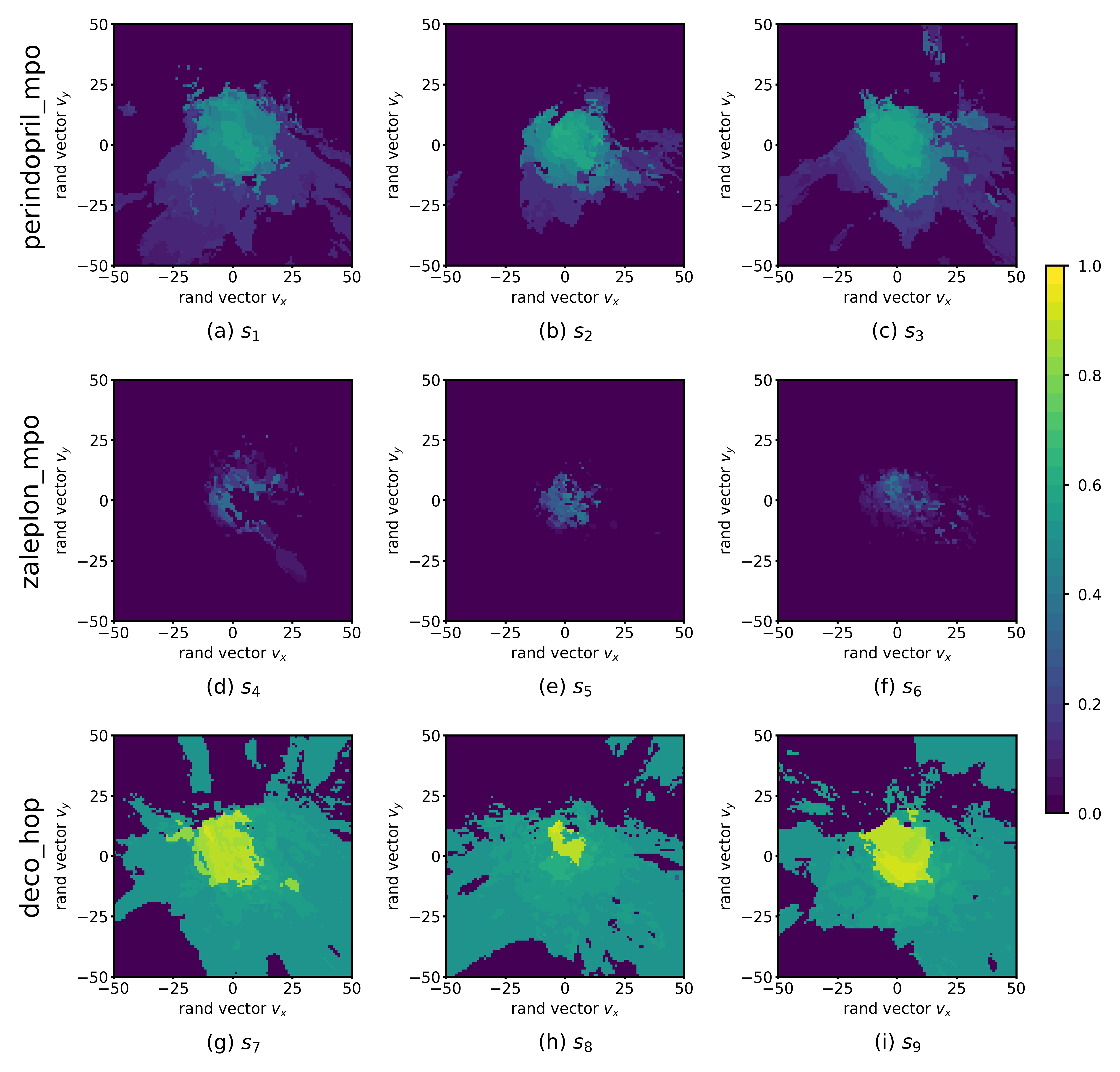
Figure 1: Function landscapes for various optimized molecules found by QMO. SMILES strings are listed in Appendix B.2.

Fig. 1 shows the function landscapes of the selected Guacamol objectives. The origin corresponds to an optimized latent vector found by QMO, and the vector is perturbed along two random directions $v_{x}$ and $v_{y}$ sampled from the uniform distribution on the unit sphere.

As shown, the zaleplon_mpo task has the smallest central area consisting of high scoring molecules and a relatively flat landscape elsewhere, meaning that the QMO optimizer needs to traverse a very flat unfavorable region to enter a very small optimal neighborhood. This matches the observation that zaleplon_mpo is a highly difficult task. The deco_hop task, while not nearly as difficult of a task, still exhibits a very discrete jump in values around the central region, which makes it more difficult for the QMO optimizer to find the true optimal neighborhood. Finally, perindopril_mpo appears to be the most smooth function. The optimal central area is larger than for zaleplon_mpo, and the discrete jumps in function values are not as large as in the other tasks.

4.2 Convergence of ZO optimization methods

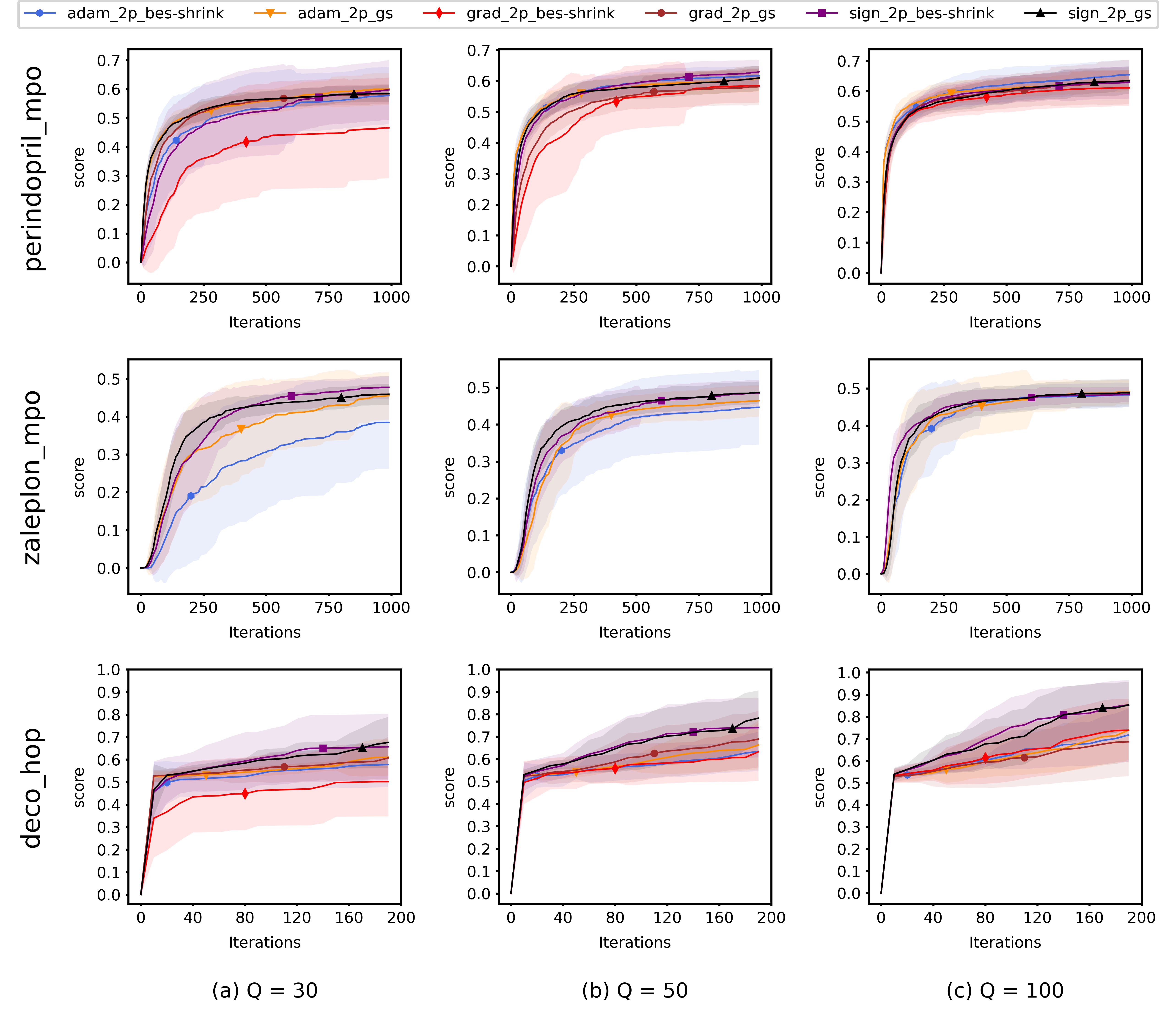
Figure 2: Convergence of QMO with different ZO optimizers.

Fig. 2 shows the results from experiments run using QMO only and compares the convergence of ZO optimization methods with different $Q$. Here, adam_2p_bes-shrink refers to QMO using the ZO-Adam optimizer with the 2-point BeS-shrink gradient estimator (QMO-Adam-2p-BeS-shrink), and similarly for the other ZO optimization methods. Diversity scores of the molecules found by QMO are reported in Appendix B.3.

Overall, the results indicate that ZO-signGD is not only the most query-efficient method, but also the most robust to difficult function landscapes of molecular objectives. Compared with ZO-Adam, ZO-signGD converges with both higher speed and better accuracy for most settings, and the difference is especially clear for low $Q$ and less smooth functions like zaleplon_mpo and deco_hop. The improved convergence accuracy of ZO-signGD compared to ZO-Adam is particularly interesting as ZO-Adam converges with much greater accuracy in other problems like adversarial example generation [14], thus showing the challenges presented by molecular objectives and the improved robustness of ZO-signGD to their function landscapes.

Finally, as a note, both ZO-Adam and ZO-signGD outperform ZO-GD. In fact, ZO-GD is completely unsuccessful for the zaleplon_mpo task: even when searching a wide range of hyperparameters and testing several molecules, ZO-GD is unable to find any molecules with zaleplon_mpo scores above 0.2 within the first 100 iterations, and often cannot even get above 0.01. Inspection revealed that the gradient vectors were too small for ZO-GD to make meaningful point updates. Thus, full zaleplon_mpo experiments were not run using ZO-GD. In addition, results from GS and BeS-shrink gradient estimators do not differ greatly, though GS seems to converge faster with lower $Q$.

4.3 Query efficiency of QMO versus other approaches

Fig. 3 shows the optimization curves when limiting optimization to a query 10K budget, including experiments run using QMO only (specifically, only QMO-sign-2p-GS is shown), baseline models only, and hybrid approaches. Precise numbers and area under curve (AUC) scores are also reported in Appendix B.4.

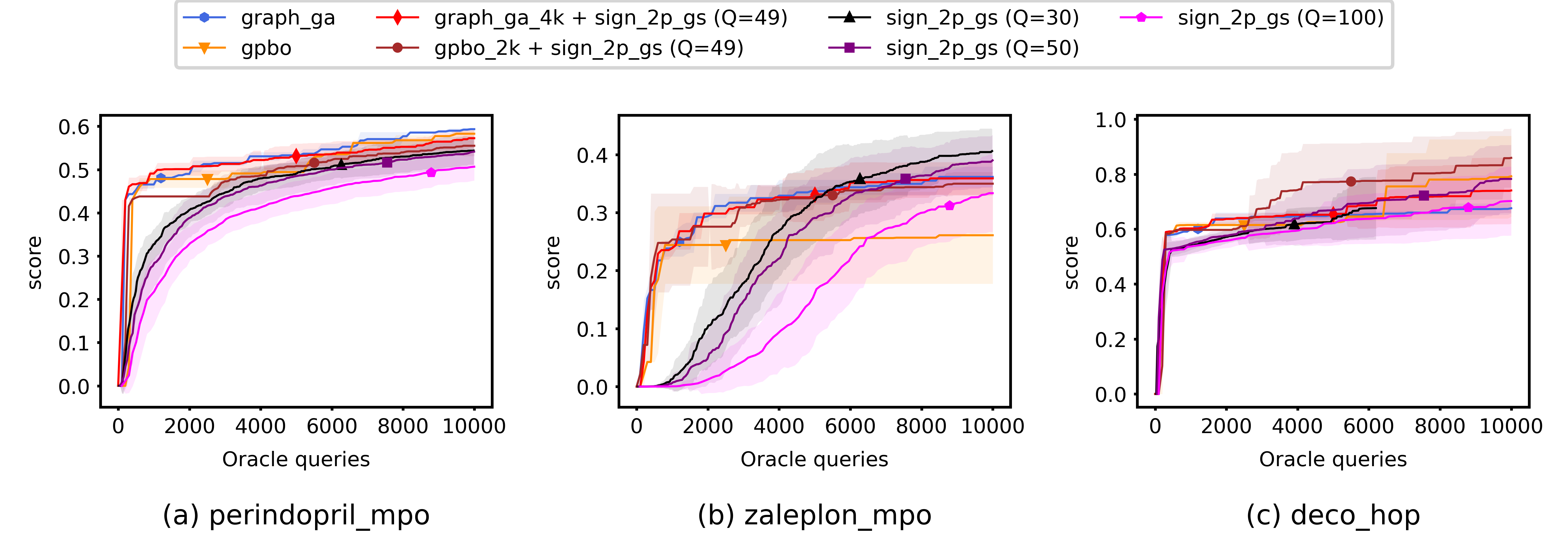
Figure 3: Optimization curves of QMO, generative models, and hybrid methods.

The baseline models (Graph-GA and GPBO) demonstrate faster convergence speed than QMO alone, and the relative convergence accuracies of all methods differ slightly for each task and can be said to be comparable overall. However, the hybrid approaches combining baseline models with QMO (i.e., Graph GA + sign_2p_gs) produce similar curves to their baseline model counterparts even for zaleplon_mpo and deco_hop, where QMO has higher convergence accuracy than the baseline models, so further investigation may be necessary to effectively integrate QMO into hybrid approaches.

5 Conclusion

In this paper, we study the application of ZO optimization methods to molecule optimization. Through experimentation on tasks from the Guacamol suite, we show that ZO-signGD outperforms ZO-Adam and ZO-GD, especially for more difficult function landscapes with small regions of optima, flat regions, and discrete jumps. Accordingly, we observe that the sign operation can increase robustness to the difficult function landscapes of molecular objectives, while also achieving higher query efficiency compared to other optimizer updating methods. We also discuss how the generic QMO framework can be applied practically in realistic drug discovery scenarios, which includes a hybrid approach with other models.

To conclude, we would like to mention a few limitations of this study. Synthesizability of molecules is not accounted for, though one possible approach is to modify the objective function with a synthesizability loss. Additionally, the effect of autoencoder choice and latent dimension are not thoroughly investigated for the selected benchmark tasks, though Hoffman et al. [8] provide analysis for their antimicrobial peptides task. Finally, while Hoffman et al. [8] also show that training an oracle prediction model (to predict scores based on latent representations) has significant disadvantages in optimization accuracy compared to always using the oracle itself, we do not thoroughly investigate the impact it would have on the objective function landscapes in the latent space.

Appendix

Appendix A Implementation details

Winter et al. [22] showed that their CDDD autoencoder model has a high validity rate of 97%, even when traversing a large distance from the valid latent representations of randomly picked molecules. In our implementation of QMO, we dealt with decode failures by assigning a penalty score of 0.1 less than the score of the starting molecule, $f(\mathbf{z}_{0})-0.1$.

Also, we only considered the molecules generated after each optimization iteration. That is, we did not consider the $Q$ molecules obtained from decoding the perturbed latent vectors $\{\mathbf{z}+\beta\mathbf{u}_{q}\}_{q=1}^{Q}$ (used for estimating gradients) in $\mathcal{Z}_{\mathrm{iterate}}$ despite that they were also used to query the oracle $\mathcal{O}$. Especially in a realistic drug discovery scenario where oracle evaluations are highly expensive, we would of course want to also consider these molecules in case they exhibit good properties. In addition, while we considered there to be $Q+1$ oracle evaluations necessary for each optimization iteration, the actual amount would be lower in practice as some of the perturbed latent vectors would decode to the same molecule since the perturbations are small (and a small number of latent vectors would also decode to no valid input).

All experiments were run using Google Colab, and code for QMO is available at: https://github.com/IBM/QMO-bench. For the Graph-GA and GPBO baseline models, we adopt the implementation of Gao et al. [10].

Appendix B Additional results

B.1 Comparing 1-point and 2-point gradient estimators

Though we ran only 2-point gradient estimators on the Guacamol tasks, we also compared 1-point gradient estimators on the QED [30] objective. Specifically, following the setup of Hoffman et al. [8], we defined a minimum similarity threshold of 0.4 (and did not consider molecules with similarity less than 0.4 to the starting molecule) and set the oracle $\mathcal{O}(x)=4\cdot\mathrm{QED}(x)-\mathrm{max}(0.4-\mathrm{sim}(x,x_{0}),0)$ for molecule $x\in\mathcal{X}$ and starting molecule $x_{0}$, where $\mathrm{sim(\cdot)}$ denotes Tanimoto similarity with Morgan fingerprints. We selected 100 molecules with QED scores in $[0.7,0.8]$ from the test set in [31] (who extracted the molecules from ZINC) and optimized each with $T=20$ iterations and 20 random restarts each. We consider an optimized molecule a success if its QED scores falls in $[0.9,1.0]$, and we visualize in Fig. B1 how many random restarts are necessary for different ZO optimization methods to achieve a given success rate. As shown, 2-point gradient estimators achieve significantly higher success rates than their 1-point counterparts given the same number of random restarts.

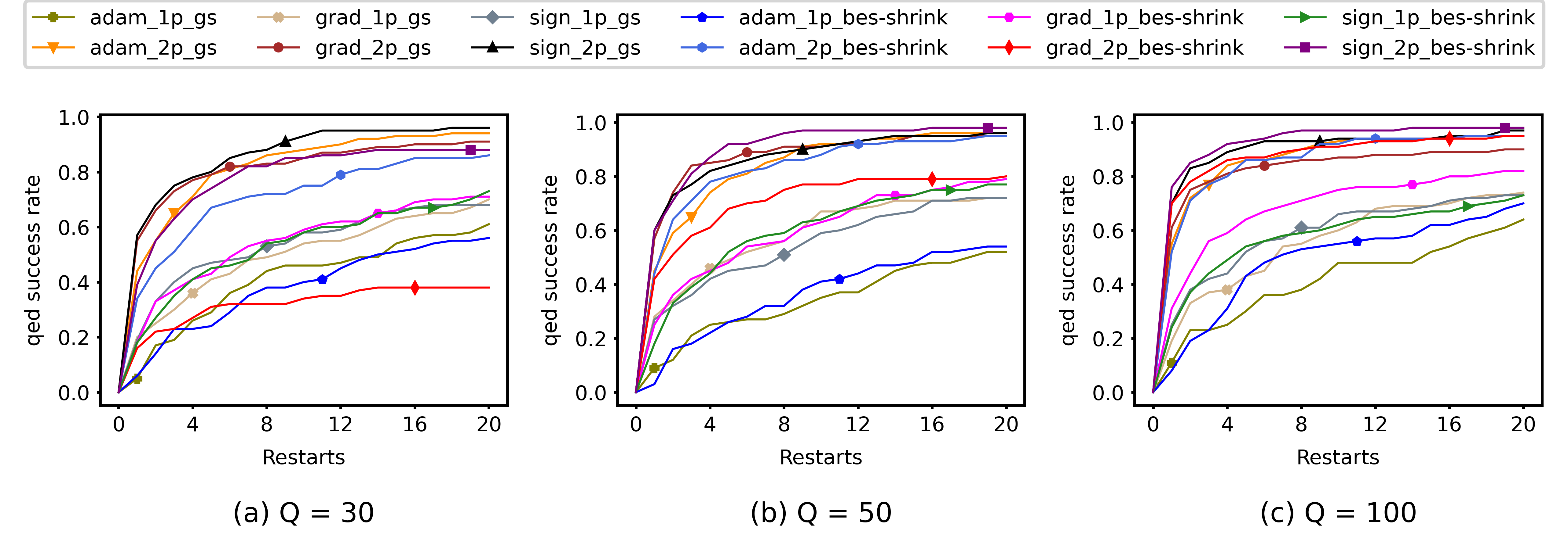
Figure B1: Optimization of QED with different ZO optimizers.

B.2 SMILES strings of molecules found by QMO

The SMILES strings from Fig. 1 are as follows:

• $s_{1}$ = CCCC(NC(C)Cn1c(C2CCCCC2)nc2cc(C(=O)O)ccc21)C(=O)OCC

• $s_{2}$ = CCCC(C(=O)OCC)c1nc2cc(C(=O)O)ccc2n1C1CCCCC1C(C)=O

• $s_{3}$ = CCCC(C)n1c(C(=O)NC(C)C(=O)OCC)cc2cc(C3CCCCC3)cc(C(=O)O)c21

• $s_{4}$ = COc1cc(C(=O)NCC23CC=CC2C3)nc2c(C#N)cccc12

• $s_{5}$ = CCC1(CC)C(C(=O)Nc2cccc(F)c2)=CN=C2C=C(C#N)C(=O)N21

• $s_{6}$ = CCC12CC(CO1)N(C(=O)c1cnc3cccc(C#N)c(=O)c3c1)C2

• $s_{7}$ = COc1cc2ncnc(Nc3ccc(F)c4ncccc34)c2cc1C(C)C

• $s_{8}$ = CCCCOc1ncccc1C(=O)CNc1ncnc2cc(OC(F)F)c(F)cc12

• $s_{9}$ = COc1cc(Nc2ncnc3cc(OC)c([N+](=O)[O-])cc23)ccc1F.

B.3 Diversity metrics

Table B1 shows the diversity of the QMO optimized molecules from Section 4.2 (optimized using sign_2p_gs with $Q=50$). For each starting molecule in the test set, the best molecule found after two random restarts was used, showing the diversity of molecules that can be generated from different starting points. Hoffman et al. [8] also showed how different random restarts starting from the same starting point can find diverse candidates.

Table B1: Diversity of 20 QMO optimized molecules from different starting points.

Task	Average score	Diversity
perindopril_mpo	0.628	0.678
zaleplon_mpo	0.500	0.805
deco_hop	0.859	0.664

B.4 Query efficiency tables

Scores from Fig. 3 are summarized below in Tables B2, B3, and B4.

Table B2: Scores for perindopril_mpo with various query budgets.

Methods	AUC	500 q	1000 q	2000 q	5000 q	10000 q
graph_ga	0.527	0.453	0.465	0.490	0.533	0.593
gpbo	0.502	0.446	0.478	0.478	0.494	0.583
sign_2p_gs ($Q=30$)	0.456	0.219	0.327	0.408	0.490	0.544
sign_2p_gs ($Q=50$)	0.441	0.176	0.284	0.388	0.485	0.541
sign_2p_gs ($Q=100$)	0.395	0.101	0.218	0.330	0.439	0.507
graph_ga_4k + sign_2p_gs ($Q=49$)	0.522	0.466	0.491	0.501	0.531	0.572
gpbo_2k + sign_2p_gs ($Q=49$)	0.487	0.435	0.438	0.438	0.508	0.555

Table B3: Scores for zaleplon_mpo with various query budgets.

Methods	AUC	500 q	1000 q	2000 q	5000 q	10000 q
graph_ga	0.315	0.167	0.239	0.294	0.337	0.362
gpbo	0.241	0.172	0.244	0.244	0.253	0.261
sign_2p_gs ($Q=30$)	0.259	0.001	0.013	0.105	0.321	0.406
sign_2p_gs ($Q=50$)	0.233	0.000	0.007	0.048	0.291	0.390
sign_2p_gs ($Q=100$)	0.158	0.000	0.000	0.013	0.168	0.333
graph_ga_4k + sign_2p_gs ($Q=49$)	0.314	0.183	0.239	0.298	0.331	0.359
gpbo_2k + sign_2p_gs ($Q=49$)	0.307	0.223	0.254	0.276	0.329	0.350

Table B4: Scores for deco_hop with various query budgets.

Methods	AUC	500 q	1000 q	2000 q	5000 q	10000 q
graph_ga	0.634	0.580	0.600	0.638	0.650	0.676
gpbo	0.663	0.587	0.615	0.615	0.626	0.792
sign_2p_gs ($Q=30$)	0.582	0.529	0.539	0.572	0.638	-
sign_2p_gs ($Q=50$)	0.652	0.529	0.548	0.576	0.669	0.783
sign_2p_gs ($Q=100$)	0.604	0.522	0.537	0.558	0.622	0.702
graph_ga_4k + sign_2p_gs ($Q=49$)	0.661	0.592	0.602	0.637	0.655	0.741
gpbo_2k + sign_2p_gs ($Q=49$)	0.716	0.591	0.597	0.597	0.772	0.859

Appendix C Other ZO optimization methods

Other than the ZO optimization methods considered here, ZO stochastic coordinate descent (ZO-SCD) [15] was also tested. However, because the coordinate-wise gradient estimator relies on perturbing coordinates individually, the perturbed vector embeddings used to estimate gradients almost always decoded back to the same molecule as the original non-perturbed vector. In other words, the autoencoder almost always perceived the embedding vectors with all coordinates the same but one coordinate to be the same molecule, so the coordinate-wise gradient estimates were almost always zero.

Appendix D Hyperparameter tuning

Aside from the number of random perturbations $Q$, there are two other main hyperparameters for each of the ZO optimization methods compared: function smoothing parameter $\beta$, and learning rate $\alpha$. The value $\beta=10$ was used for all tasks as it was found to work well with the CDDD model. Consistent with Hoffman et al. [8], we find that $\beta=1$ or below does not work well (as gradients cannot be accurately approximated without sufficient smoothing) and $\beta=100$ or above results in many decode failures. When trying a few molecules with $\beta$ values between this range (including $\beta=\{5,10,20,50\}$ for each task, $\beta=10$ still performed best for the majority of molecules. The tuning of $\alpha$ is shown in Table D1 and Table D2. As a note, $\alpha$ larger than the largest tested values for each optimization method often resulted in many decode failures, so even if the best $\alpha$ was the largest value tested, choosing notably larger $\alpha$ (greater by more than a factor of 2) may not be a good idea. Also, for ZO-Adam, two additional hyperparameters are used for the adaptive learning rate: the exponential averaging parameters $\beta_{1}$ and $\beta_{2}$. For these parameters, we use the default values used by the PyTorch Adam implementation, $\beta_{1}=0.9$ and $\beta_{2}=0.999$.

Table D1: Tuning of learning rate $\alpha$ for Guacamol tasks. Scores correspond to the average scores after optimizing 20 molecules with 2 random restarts each (40 trials total) for $T=1000$ iterations.

Task	Methods	Learning rate $\alpha$	$Q=30$	$Q=50$	$Q=100$
perindopril_mpo	adam_2p_bes-shrink	0.1	0.555	0.598	0.607
		0.2	0.578	0.617	0.635
		0.3	0.564	0.617	0.654
	adam_2p_gs	0.1	0.600	0.600	0.604
		0.2	0.589	0.611	0.635
		0.3	0.560	0.605	0.637
	grad_2p_bes-shrink	30.0	0.429	0.585	0.611
		50.0	0.466	0.555	0.598
	grad_2p_gs	2.0	0.584	0.582	0.571
		5.0	0.500	0.566	0.630
	sign_2p_bes-shrink	0.05	0.531	0.593	0.602
		0.1	0.598	0.630	0.629
		0.2	0.531	0.575	0.615
	sign_2p_gs	0.05	0.583	0.595	0.593
		0.1	0.585	0.610	0.635
		0.2	0.534	0.564	0.617
zaleplon_mpo	adam_2p_bes-shrink	0.1	0.386	0.445	0.449
		0.2	0.208	0.447	0.483
		0.3	0.151	0.376	0.470
	adam_2p_gs	0.1	0.455	0.465	0.472
		0.2	0.374	0.453	0.491
		0.3	0.321	0.425	0.483
	sign_2p_bes-shrink	0.05	0.382	0.398	0.429
		0.1	0.478	0.485	0.477
		0.2	0.410	0.445	0.485
	sign_2p_gs	0.05	0.436	0.442	0.429
		0.1	0.460	0.487	0.488
		0.2	0.399	0.441	0.483
deco_hop	adam_2p_bes-shrink	0.1	0.544	0.564	0.605
		0.2	0.578	0.636	0.722
		0.3	0.585	0.628	0.738
	adam_2p_gs	0.1	0.564	0.585	0.603
		0.2	0.603	0.638	0.735
		0.3	0.612	0.669	0.741
	grad_2p_bes-shrink	50.0	0.480	0.587	0.666
		70.0	0.508	0.634	0.739
	grad_2p_gs	2.0	0.554	0.544	0.543
		5.0	0.608	0.597	0.584
		7.0	0.596	0.681	0.653
		10.0	0.592	0.696	0.688
	sign_2p_bes-shrink	0.1	0.645	0.709	0.784
		0.2	0.663	0.748	0.860
		0.3	0.613	0.670	0.746
	sign_2p_gs	0.1	0.676	0.763	0.762
		0.2	0.657	0.783	0.865
		0.3	0.616	0.621	0.763

Table D2: Tuning of learning rate $\alpha$ for QED task. Scores correspond to the average of the success rates of optimizing 100 molecules after 1, 5, and 20 random restarts with $T=20$ iterations per restart.

Methods	Learning rate $\alpha$	$Q=30$	$Q=50$	$Q=100$
adam_1p_bes-shrink	0.05	0.007	0.013	0.050
	0.1	0.193	0.193	0.290
	0.2	0.287	0.277	0.403
adam_1p_gs	0.05	0.003	0.010	0.030
	0.1	0.180	0.20	0.237
	0.2	0.317	0.290	0.350
adam_2p_bes-shrink	0.05	0.187	0.363	0.497
	0.1	0.443	0.577	0.730
	0.2	0.623	0.730	0.777
adam_2p_gs	0.05	0.337	0.400	0.507
	0.1	0.627	0.707	0.777
	0.2	0.723	0.733	0.787
grad_1p_bes-shrink	0.5	0.053	0.070	0.123
	1.5	0.440	0.507	0.590
grad_1p_gs	0.1	0.420	0.243	0.100
	0.2	0.437	0.497	0.453
	0.5	0.120	0.220	0.323
grad_2p_bes-shrink	10.0	0.137	0.357	0.767
	20.0	0.283	0.633	0.840
grad_2p_gs	0.2	0.103	0.090	0.087
	0.5	0.350	0.323	0.260
	1.5	0.750	0.770	0.743
	2.0	0.697	0.793	0.780
sign_1p_bes-shrink	0.05	0.010	0.027	0.040
	0.1	0.257	0.287	0.317
	0.2	0.453	0.490	0.503
sign_1p_gs	0.05	0.000	0.017	0.010
	0.1	0.173	0.270	0.287
	0.2	0.447	0.480	0.500
sign_2p_bes-shrink	0.05	0.177	0.360	0.510
	0.1	0.497	0.723	0.810
	0.2	0.670	0.833	0.890
sign_2p_gs	0.05	0.293	0.373	0.483
	0.1	0.677	0.730	0.813
	0.2	0.777	0.800	0.860

Appendix E Licenses

All test sets of molecules were originally extracted from the ZINC database [29] which is free for use by anyone.

References

- Olivecrona et al. [2017] Marcus Olivecrona, Thomas Blaschke, Ola Engkvist, and Hongming Chen. Molecular de-novo design through deep reinforcement learning. Journal of cheminformatics, 9(1):1–14, 2017.
- Jensen [2019] Jan H Jensen. A graph-based genetic algorithm and generative model/monte carlo tree search for the exploration of chemical space. Chemical science, 10(12):3567–3572, 2019.
- Tripp et al. [2021] Austin Tripp, Gregor NC Simm, and José Miguel Hernández-Lobato. A fresh look at de novo molecular design benchmarks. In NeurIPS 2021 AI for Science Workshop, 2021.
- Gómez-Bombarelli et al. [2018] Rafael Gómez-Bombarelli, Jennifer N Wei, David Duvenaud, José Miguel Hernández-Lobato, Benjamín Sánchez-Lengeling, Dennis Sheberla, Jorge Aguilera-Iparraguirre, Timothy D Hirzel, Ryan P Adams, and Alán Aspuru-Guzik. Automatic chemical design using a data-driven continuous representation of molecules. ACS central science, 4(2):268–276, 2018.
- Jin et al. [2018a] Wengong Jin, Regina Barzilay, and Tommi Jaakkola. Junction tree variational autoencoder for molecular graph generation. In International conference on machine learning, pages 2323–2332. PMLR, 2018a.
- Brown et al. [2019] Nathan Brown, Marco Fiscato, Marwin HS Segler, and Alain C Vaucher. Guacamol: benchmarking models for de novo molecular design. Journal of chemical information and modeling, 59(3):1096–1108, 2019.
- García-Ortegón et al. [2022] Miguel García-Ortegón, Gregor NC Simm, Austin J Tripp, José Miguel Hernández-Lobato, Andreas Bender, and Sergio Bacallado. Dockstring: easy molecular docking yields better benchmarks for ligand design. Journal of chemical information and modeling, 62(15):3486–3502, 2022.
- Hoffman et al. [2022] Samuel C Hoffman, Vijil Chenthamarakshan, Kahini Wadhawan, Pin-Yu Chen, and Payel Das. Optimizing molecules using efficient queries from property evaluations. Nature Machine Intelligence, 4(1):21–31, 2022.
- Tripp et al. [2022] Austin Tripp, Wenlin Chen, and José Miguel Hernández-Lobato. An evaluation framework for the objective functions of de novo drug design benchmarks. In ICLR2022 Machine Learning for Drug Discovery, 2022.
- Gao et al. [2022] Wenhao Gao, Tianfan Fu, Jimeng Sun, and Connor W Coley. Sample efficiency matters: A benchmark for practical molecular optimization. arXiv preprint arXiv:2206.12411, 2022.
- Liu et al. [2018] Sijia Liu, Pin-Yu Chen, Xiangyi Chen, and Mingyi Hong. signsgd via zeroth-order oracle. In International Conference on Learning Representations, 2018.
- Liu et al. [2020] Sijia Liu, Pin-Yu Chen, Bhavya Kailkhura, Gaoyuan Zhang, Alfred O Hero III, and Pramod K Varshney. A primer on zeroth-order optimization in signal processing and machine learning: Principals, recent advances, and applications. IEEE Signal Processing Magazine, 37(5):43–54, 2020.
- Nesterov and Spokoiny [2017] Yurii Nesterov and Vladimir Spokoiny. Random gradient-free minimization of convex functions. Foundations of Computational Mathematics, 17(2):527–566, 2017.
- Chen et al. [2019] Xiangyi Chen, Sijia Liu, Kaidi Xu, Xingguo Li, Xue Lin, Mingyi Hong, and David Cox. Zo-adamm: Zeroth-order adaptive momentum method for black-box optimization. Advances in Neural Information Processing Systems, 32, 2019.
- Lian et al. [2016] Xiangru Lian, Huan Zhang, Cho-Jui Hsieh, Yijun Huang, and Ji Liu. A comprehensive linear speedup analysis for asynchronous stochastic parallel optimization from zeroth-order to first-order. Advances in Neural Information Processing Systems, 29, 2016.
- Li et al. [2022] Zichong Li, Pin-Yu Chen, Sijia Liu, Songtao Lu, and Yangyang Xu. Zeroth-order optimization for composite problems with functional constraints. In Proceedings of the AAAI Conference on Artificial Intelligence, volume 36, pages 7453–7461, 2022.
- Kornowski and Shamir [2021] Guy Kornowski and Ohad Shamir. Oracle complexity in nonsmooth nonconvex optimization. Advances in Neural Information Processing Systems, 34:324–334, 2021.
- Chen et al. [2017] Pin-Yu Chen, Huan Zhang, Yash Sharma, Jinfeng Yi, and Cho-Jui Hsieh. Zoo: Zeroth order optimization based black-box attacks to deep neural networks without training substitute models. In Proceedings of the 10th ACM workshop on artificial intelligence and security, pages 15–26, 2017.
- Tu et al. [2019] Chun-Chen Tu, Paishun Ting, Pin-Yu Chen, Sijia Liu, Huan Zhang, Jinfeng Yi, Cho-Jui Hsieh, and Shin-Ming Cheng. Autozoom: Autoencoder-based zeroth order optimization method for attacking black-box neural networks. In Proceedings of the AAAI Conference on Artificial Intelligence, volume 33, pages 742–749, 2019.
- Dhurandhar et al. [2019] Amit Dhurandhar, Tejaswini Pedapati, Avinash Balakrishnan, Pin-Yu Chen, Karthikeyan Shanmugam, and Ruchir Puri. Model agnostic contrastive explanations for structured data. arXiv preprint arXiv:1906.00117, 2019.
- Weininger [1988] David Weininger. Smiles, a chemical language and information system. 1. introduction to methodology and encoding rules. Journal of chemical information and computer sciences, 28(1):31–36, 1988.
- Winter et al. [2019] Robin Winter, Floriane Montanari, Frank Noé, and Djork-Arné Clevert. Learning continuous and data-driven molecular descriptors by translating equivalent chemical representations. Chemical science, 10(6):1692–1701, 2019.
- Flaxman et al. [2005] Abraham D Flaxman, Adam Tauman Kalai, and H Brendan McMahan. Online convex optimization in the bandit setting: gradient descent without a gradient. In Proceedings of the sixteenth annual ACM-SIAM symposium on Discrete algorithms, pages 385–394, 2005.
- Gao and Sener [2022] Katelyn Gao and Ozan Sener. Generalizing gaussian smoothing for random search. In International Conference on Machine Learning, pages 7077–7101. PMLR, 2022.
- Bernstein et al. [2018] Jeremy Bernstein, Yu-Xiang Wang, Kamyar Azizzadenesheli, and Animashree Anandkumar. signsgd: Compressed optimisation for non-convex problems. In International Conference on Machine Learning, pages 560–569. PMLR, 2018.
- Kingma and Ba [2015] Diederik P Kingma and Jimmy Ba. Adam: A method for stochastic optimization. In International Conference on Learning Representations, 2015.
- Balles and Hennig [2018] Lukas Balles and Philipp Hennig. Dissecting adam: The sign, magnitude and variance of stochastic gradients. In International Conference on Machine Learning, pages 404–413. PMLR, 2018.
- Srinivas et al. [2010] Niranjan Srinivas, Andreas Krause, Sham Kakade, and Matthias Seeger. Gaussian process optimization in the bandit setting: no regret and experimental design. In Proceedings of the 27th International Conference on Machine Learning, pages 1015–1022, 2010.
- Sterling and Irwin [2015] Teague Sterling and John J Irwin. Zinc 15–ligand discovery for everyone. Journal of chemical information and modeling, 55(11):2324–2337, 2015.
- Bickerton et al. [2012] G Richard Bickerton, Gaia V Paolini, Jérémy Besnard, Sorel Muresan, and Andrew L Hopkins. Quantifying the chemical beauty of drugs. Nature chemistry, 4(2):90–98, 2012.
- Jin et al. [2018b] Wengong Jin, Kevin Yang, Regina Barzilay, and Tommi Jaakkola. Learning multimodal graph-to-graph translation for molecule optimization. In International Conference on Learning Representations, 2018b.