Sequential hypothesis testing for Axion Haloscopes

Abstract

The goal of this paper is to introduce a novel likelihood-based inferential framework for axion haloscopes which is valid under the commonly applied “rescanning” protocol. The proposed method enjoys short data acquisition times and a simple tuning of the detector configuration. Local statistical significance and power are computed analytically, avoiding the need of burdensome simulations. Adequate corrections for the look-elsewhere effect are also discussed. The performance of our inferential strategy is compared with that of a simple method which exploits the geometric probability of rescan. Finally, we exemplify the method with an application to a HAYSTAC type axion haloscope.

1.   Introduction

The existence of dark matter was first postulated almost a century ago [1] and is today a well-established paradigm in astrophysics and cosmology. However, its detection and identification on a fundamental level is still one of the most investigated problems across all physical sciences [2, 3, 4, 5, 6, 7, 8]. Among the plethora of viable particle candidates which may constitute dark matter, axions are some among the most appealing ones. In fact, they were originally theorized in relation to the strong CP problem of fundamental physics [9, 10, 11, 12]. Only later, physicists realized axions exhibit properties that are consistent with those of cold dark matter and their behavior is compatible with cosmological and astrophysical constraints [13, 14, 15] — see [16, 17, 18] for recent reviews.

At present, the experimental effort towards a direct detection is witnessing many experiments being planned or already running [19, 20, 21, 22, 23, 24]. One of the most well-established way to search for axions is through cavity microwave experiments, generally referred to as haloscopes. The idea was first proposed by Sikivie in 1985 [25]; it relies on the Primakoff effect [26] to induce the axion-to-photon conversion in a resonant apparatus by matching the Compton wavelength of the axion and the resonant mode of the cavity. The interaction appears as power being deposited at a frequency matching the axion mass, i.e. $\nu_{a}=m_{a}c^{2}h^{-1}$.

Since the axion frequency $\nu_{a}$ is unknown a priori, a standard axion experiment is conceptually run by sequentially tuning the detector over the available frequencies. The goal is that of identifying a peak emerging from the fluctuations in the noise power of the system. The ratio between the power deposited by the axion over the noise power determines the signal-to-noise ratio, which is directly linked to the sensitivity and improves with the time invested measuring. As a result, the extent to which an axion experiment is able to explore the parameter space does not depend just on the detector properties and the available resources, such as the total lifetime, but also on the way those resources are effectively allocated. In fact, while experimenters could (in principle) focus solely on one specific frequency and increase the signal-to-noise ratio arbitrarily, they have also the freedom to carefully evaluate the fluctuations measured over multiple frequencies and repeat the measurement only for those those deemed to provide promising hints of an axion. It follows that the choice of such protocol for both data acquisition and statistical analyses is crucial.

Despite a variety of protocols have been proposed [27, 28, 29, 30, e.g.,], the main source of disagreement across different experiments is how to flag plausible candidate frequencies to be rescanned. This especially true when aiming to perform an analysis in a frequentist framework.

In this manuscript, we aim to address this inconsistency by introducing a statistically rigorous, likelihood-based, rescan protocol which provides the tools needed for a direct comparison of the results of future experiments, such as the reachable sensitivity, or upper limits on the axion-photon coupling. We believe that this is especially needed given that there is no general consensus on the way such quantities are defined within the community.

The proposed inferential framework is presented in Sections 2-4. In order to ease the exposition, the main elements of the procedure are introduced in a step-by-step manner, gradually increasing level of complexity. Specifically, in Section 2, we outline the frequentist likelihood-based approach for axion searches in the simple scenario where only one scan is performed at a given frequency. In Section 3, we introduce the re-scan protocol, i.e., we allow our measurements to be conducted sequentially, over multiple scans at a fixed frequency. This is the main methodological result of the article. In Section 4, we discuss adequate “look-elsewhere effect” (LEE) corrections. That is, we allow the re-scan protocol to be performed over multiple frequencies. Hence, adequate LEE adjustments are introduced in order to control the probability of a false discovery over the entire frequency range considered. Section 5 outlines how to set upper limits in the context of a real axion experiment. Specifically, we use the parameterized properties of the first phase of HAYSTAC detector [31, 32] to make a projection of the reachable upper limit on the photon-axion coupling constant, showing how different definitions can affect the final result. A summary and concluding remarks are presented in Section 6.

2.   Likelihood-based inference

In what follows, we assume that the sensitivity domain of a given axion experiment is discretized into $M$ bins, each one of them marking a frequency $\nu_{i}$, idexed by the subscript $i=1,\,\dots,\,M$. The measuring process associates to the $i$-th bin a set of $y_{ij}$ normalized noise fluctuations, possibly taken under different detector configurations $j=1,\dots,\,N_{i}$. We assume the fluctuations $y_{ij}$ to be normally distributed with unknown mean, $\mu_{ij}$, and known standard deviation, $\sigma_{ij}$, i.e.,

$$y_{ij}\sim\mathcal{N}(\mu_{ij},\,\sigma_{ij}).$$ (1)

The normality assumption in (1) simplifies the calculations and is a reasonable approximation of the true distribution of the noise fluctuations [33, 34, 35, e.g.,]. In Equation (1), the mean $\mu_{ij}$ is nonzero only if an axion deposits power proportional to some coupling, $A$, on the $i$-th frequency bin, i.e.,

$$\mu_{ij}=A\,w_{ij}.$$ (2)

Here, $A$ is the parameter of interest and the weights $w_{ij}$ are assumed to be known — see for instance Equation (42) in Section 5 or Ref. [36]. The main goal of the proposed analysis is that of testing the hypotheses

$$H_{0}:A=0\quad\text{versus}\quad H_{1}:A\neq 0;$$ (3)

that is, we aim to assess if the null hypothesis, $H_{0}$, of no axion is consistent with the observations collected by the detector.

Denote with $Y_{t}=\{y_{i1},\dots,y_{iN_{i}}\}_{i\in\mathcal{I}_{t}}$ the sets of fluctuations relevant to check for the presence of an axion at a frequency $\nu_{t}$, with $t=1,\,\dots,\,T$, and $T\leq M$. Specifically, $Y_{t}$ collects all the normalized noise fluctuations measured across all the $N_{i}$ detector configurations at frequencies $\nu_{i}$ in a neighborhood $\mathcal{I}_{t}$ of $\nu_{t}$. From (1) it follows that the likelihood function is

$$\mathcal{L}_{t}(A)=\prod_{i\in\mathcal{I}_{t}}\prod_{j=1}^{N_{i}}\phi(y_{ij};\,Aw_{ij},\sigma_{ij}),$$ (4)

where $\phi(\>\cdot\>;\,Aw_{ij},\,\sigma_{ij})$ denotes the density of a normal with mean $Aw_{ij}$ and standard deviation $\sigma_{ij}$.

We begin by investigating the case where the presence of an axion is tested at a given frequency $\nu_{t}$. In order to simplify the notation, the subscript $t$ is dropped in the remainder of this section and in Section 3. It will be reintroduced in Section 4, when discussing the situation where multiple tests conducted simultaneously over different frequencies.

The statistic we rely upon to test (3) is the signed-root likelihood ratio test [37, e.g.,]. When testing the hypotheses in (3), it specifies as

$$s=\frac{x}{\sqrt{u}},$$ (5)

where

$$x=\sum_{i\in\mathcal{I}}\sum_{j=1}^{N_{i}}\frac{w_{ij}y_{ij}}{\sigma_{ij}^{2}}\quad\text{and}\quad u=\sum_{i\in\mathcal{I}}\sum_{j=1}^{N_{i}}\frac{w_{ij}^{2}}{\sigma_{ij}^{2}}.$$ (6)

Here, $u$ summarizes the various detector configurations, with no need to further transform and rescale the original data $y_{ij}$, which are now aliased by the (one-dimensional) random variable $x$. Being a linear combination of normally distributed random variables, $x$ is also Gaussian with variance $\sigma_{x}^{2}=u$ and mean $\mu_{x}=Au$. The latter is valid assuming the most favorable case, i.e. the hypothesis of an axion lying on the frequency being tested. In fact, we may expect that, on a given frequency bin, an axion with (true) frequency $\nu_{a}$ and coupling constant $A$ deposits the same power of an axion with (slightly shifted) frequency $\nu_{a}^{\prime}$ and coupling constant $A^{\prime}=Aw_{ij}^{\prime}/w_{ij}$.

Under $H_{0}$ in (3), the distribution of the test statistic $s$ in (5) is that of a standard normal. Whereas, if $H_{0}$ is false, then a mean shift is introduced. Once an experimental value $\hat{s}$ is measured, the significance of the departure from the null hypothesis of zero mean can be quantified by computing the p-value

$$P(s\geq\hat{s}\,|\,H_{0})=1-\Phi\left(\hat{s}\right),$$ (7)

where $\Phi\left(\cdot\right)$ is the cumulative distribution function of a standard Gaussian. When the probability (7) is below a pre-determined significance, typically denoted by $\alpha$, then $H_{0}$ is rejected and a discovery is claimed. Conventionally, the line is drawn at $5\sigma$ significance which corresponds to $\alpha=1-\Phi(5)=$2.87\text{\times}{10}^{-7}$$. In the following, we will refer to this as the statistical discovery condition, neglecting any additional procedure such as the “manual interrogation” of persistent candidates [35, 34].

3.   The rescan protocol

We now extend the experimental freedom by introducing the option to flag promising noise fluctuations as potential candidates, and increase the data sample with subsequent measurements. Additional measurements are done sequentially, until the fluctuation disappears or a discovery is claimed. Here, we will consider two main methods, the so-called geometric test (and adequate generalizations), and our likelihood-based rescan protcol. As it will become clear in Sections 3.1-3.2, the former is essentially equivalent to the frequentist framework discussed in [29], whereas the latter is new, and allows us to include additional information into the analysis.

3.1.   The geometric approach

A rather simple procedure to test for the presence of an axion is sketched in Figure 1. The inputs required are the desired significance level, $\alpha$, needed to claim a discovery, and the probability of performing an additional scan.

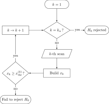
Figure 1: Flowchart of the rescan protocol based on the geometric test (Section 3.1). Its outcomes are either success (or fail) in rejecting $H_{0}$ and claiming (or not) the axion discovery.

Specifically, denote with $y_{ij\ell}$ the fluctuation measured on bin $i$, under the $j$-th detector configuration during the $\ell$-th session of measurement, or rescan. Let $x_{\ell}$ be the value of $x$ in (6) observed at the $\ell$-th scan, i.e.,

$$x_{\ell}=\sum_{i\in\mathcal{I}}\sum_{j=1}^{N_{i}}\frac{w_{ij\ell}y_{ij\ell}}{\sigma_{ij\ell}^{2}}.$$ (8)

Similarly to Section 2, we assume that the $x_{\ell}$ are independent and normally distributed with mean depending on the coupling constant $A$, i.e., $\mu_{x_{\ell}}=Au_{\ell}$, and variance

$$u_{\ell}=\sum_{i\in\mathcal{I}}\sum_{j=1}^{N_{i}}\frac{w^{2}_{ij\ell}}{\sigma^{2}_{ij\ell}}.$$ (9)

The $(\ell+1)$-th scan is performed if the condition

$$x_{\ell}>x_{\text{thr}}$$ (10)

is verified for some pre-determined threshold $x_{\text{thr}}$. The latter can be chosen, for example, to ensure that the probability of rescan when no axion is present (under $H_{0}$) is $5\%$, i.e.,

$$P(x_{\ell}>x_{\text{thr}}|H_{0})=0.05.$$ (11)

We then proceed by considering the total number of scans being performed, $K$, as our test statistic. Specifically, (10) implies that additional measurements are collected until such conditions no longer holds. Hence, $K$ can be treated as a geometric random variable with probability of “success” given by the complement of (11). Notice that, in this context a “success” corresponds to the even of stopping the procedure. We can then reject the null hypothesis of “no axion” whenever the rescan protocol based on (10) leads to $k$ scans, with $k$ satisfying

$$P(K\geq k|H_{0})=[P(x_{\ell}>x_{\text{thr}}|H_{0})]^{(k-1)}\leq\alpha.$$ (12)

Notice that $K$ differs from $k$ in that the former is a random variable taking values $k\in\{1,\dots,\infty\}$. Therefore, the number $k$ of rescans reached in a given experiment is simply the value of $K$ observed.

The geometric test above can be further extended by allowing the threshold $x_{\text{thr}}$ to vary at each scan. This effectively reduces to the frequentist approach discussed in Ref. [29] and for which (12) generalizes to

$$P(K\geq k)=\prod_{\ell=1}^{k-1}\left[P(x_{\ell}>x^{(\ell)}_{\text{thr}}|H_{0})\right]\leq\alpha$$ (13)

with $x^{(\ell)}_{\text{thr}}$ denoting the pre-determined threshold for the $\ell$-th scan.

It is worth emphasizing that (12)-(13) allow us to determine the minimum number of scans, hereafter denoted by $k_{\alpha}$, needed to claim a discovery at the prescribed significance level, $\alpha$, and for a given set of threshold(s) $x^{(\ell)}_{\text{thr}}$. Alternatively, when the resources available strongly limit the maximum number of measurements that can be performed, one can tune the threshold(s) $x^{(\ell)}_{\text{thr}}$ to ensure that (13) is verified for a pre-determined value of $k_{\alpha}$.

3.2.   The likelihood-based rescan protcol

Despite the simplicity of the approach outlined in Section 3.1, its main limitation is that it requires us to perform at least $k_{\alpha}-1$ measurements in order to claim a statistical discovery. Moreover, as noted in [29], a design based on binary outcomes like (10) is blind to the actual magnitude of the fluctuations, leading to a waste of potentially valuable information. Here, we outline a novel procedure which allows us to overcome these limitations. Additional advantages in terms of power and number of rescans needed to claim a statistical discovery are discussed in Section 3.3.

The main steps of our proposed procedure are summarized in Figure 2. We refer to this approach as likelihood-based rescan protcol and it consists of the following.

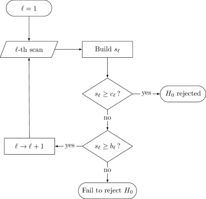
Figure 2: Flowchart of the likelihood-based rescan protocol discussed in Section 3.2. The possible outcomes are the same as the geometric test (Figure 1).

Let $k_{\alpha}$ be the maximum number of scan to be performed. For example, as noted at the end of Section 3.1, $k_{\alpha}$ can be chosen on the basis of the resources available, or to ensure a significance level of $\alpha$ using the geometric approach. Recall that $Y_{h}$ denotes the set of fluctuations relevant to check for the presence of an axion at a frequency $\nu_{t}$ in the $h$-th scan. At the $\ell$-th scan, $\ell=1,\dots,k_{\alpha}$, we compute the test statistic $s_{\ell}$ considering the set of measurements, $\bigcup_{h=1}^{\ell}Y_{h}$. The updated test statistic $s_{\ell}$ generalizes $s$ in (5) in that

$$s_{\ell}=\frac{\sum_{h=1}^{\ell}x_{h}}{\sqrt{\sum_{h=1}^{\ell}u_{h}}},$$ (14)

with $x_{h}$ and $u_{h}$ calculated as in (8) and (9), respectively, for each of the $h=1,\dots,\ell$ scans. We then rely on two conditions to determine whether or not a statistical discovery should be claimed, or if an additional scan should be performed.

Specifically, for a suitably chosen set of constants $\{c_{\ell}\}_{\ell=1}^{k_{\alpha}}$, once the $\ell$-th scan has been completed, we first assess if the condition

$$C_{\ell}=\{s_{\ell}\geq c_{\ell}\}$$ (15)

is verified. If it is, a discovery claim is made. Whereas, if $C_{\ell}$ does not hold, we verify the validity of the condition

$$B_{\ell}=\{s_{\ell}\geq b_{\ell}\},$$ (16)

where $b_{\ell}$ is the $\ell$-th elements of a set of constants $\{b_{\ell}\}_{\ell=1}^{k_{\alpha}}$, used to control the probability of rescan. If $B_{\ell}$ in (16) holds, we proceed with another rescan; if $B_{\ell}$ is not verified, the experiment is stopped, and we declare no discovery. Note that in (15) and (16) we are implicitly setting $b_{\ell}\leq c_{\ell}$, with equality holding for $\ell=k_{\alpha}$ in order to have a definite outcome. It follows that, in our likelihood-based protocol, condition (16) plays the same role as (10) in the geometric approach. Conversely from the latter, however, by combining $B_{\ell}$ and $C_{\ell}$, we allow researchers to claim a statistical discovery at any step, determining a potential break in the procedure even before reaching the $k_{\alpha}$-th scan.

Clearly, the statistical validity of the proposed strategy depends entirely on the specification of the constants $b_{\ell}$ and $c_{\ell}$. These must be chosen to ensure that the probability of a false discovery over multiple scans is no lower than the pre-determined significance level $\alpha$. This can be done as follows.

Denote with $D_{\ell}$ the event of claiming a statistical discovery at the $\ell$-th scan. On the basis of the scheme in Figure 2, such event specifies as

$$D_{\ell}=\left[\bigcap_{h=1}^{\ell-1}\left\{C_{h}^{c}\cap B_{h}\right\}\right]\cap C_{\ell},$$ (17)

with $C_{h}^{c}=\{s_{h}<c_{h}\}$. To ensure that the probability of a false discovery is indeed equal to the desired level $\alpha$, we must guarantee that

$$P\left(\bigcup_{\ell=1}^{k_{\alpha}}D_{\ell}\middle|\,H_{0}\right)=\sum_{\ell=1}^{k_{\alpha}}P\left(D_{\ell}\middle|\,H_{0}\right)=\alpha,$$ (18)

where the first equality follows from the fact that the events $D_{\ell}$ are mutually exclusive, i.e. their intersection is empty. Therefore, it is sufficient to choose $b_{\ell}$ and $c_{\ell}$ such that

$$P(D_{\ell}|\,H_{0})=\frac{\alpha}{k_{\alpha}}$$ (19)

for all $\ell=1,\dots,k_{\alpha}$ to ensure that (18) holds.

Interestingly, condition (19) can easily be expressed in closed form and thus one can exploit the latter to derive the constants $b_{\ell}$ and $c_{\ell}$ sequentially.

Specifically, for $\ell=1$, the setup is the same as that outlined in Section 2. From (7), it follows that

$$P(D_{1}|\,H_{0})=P(s_{1}\geq c_{1}|\,H_{0})=1-\Phi(c_{1})=\frac{\alpha}{k_{\alpha}},$$ (20)

and thus, $c_{1}$ is simply the quantile of order $1-\alpha$ of a standard normal. The threshold $b_{1}$, can be determined by solving the equation

$$\int_{b_{1}}^{c_{1}}\differential{s_{1}}\mathcal{N}\left(s_{1}\,\middle|\,0,1\right)=q_{1},$$ (21)

where $q_{1}$ is the probability of engaging in the second scan under the background-only hypothesis. For example, similarly to (11), we may chose $q_{1}=0.05$.

Let us extend the reasoning to the less trivial case of $\ell>1$. Since the constants $b_{\ell}$ and $c_{\ell}$ are computed sequentially, it follows that, at the $\ell$-th scan, $b_{h}$ and $c_{h}$ are known for all $h\leq\ell-1$. Define $\bm{x}=(x_{1},\,x_{2},\,\dots,x_{\ell})$ to be the vector of powers $x_{h}$ computed as in (8) for each of the $\ell$ scans. Similarly, denote with $\bm{u}=(u_{1},\,u_{2},\,\dots,u_{\ell})$ the vector collecting the respective configurations $u_{h}$ in (9). Analogously, we can define the vector of test statistics $\bm{s}=(s_{1},\,s_{2},\,\dots,s_{\ell})$, each computed as in (14). We can then easily derive the joint probability density function (pdf) of the random vector $\bm{s}$ starting from that of $\bm{x}$, and which follows a multivariate normal of dimension $\ell$, i.e.,

$$\bm{x}\sim\mathcal{N}_{\ell}\left(\bm{\mu_{x}},\,\bm{\Sigma_{x}}\right)$$ (22)

with

$$\bm{\mu_{x}}=A\bm{u}\quad\text{and}\quad\bm{\Sigma_{x}}=\text{diag}(\bm{u}).$$ (23)

Denote with $\bm{J}$ the Jacobian of the transformation in (14) that allows us to link the vectors $\bm{x}$ and $\bm{s}$. From (22), it follows that

$$\bm{s}\sim\mathcal{N}_{\ell}\left(\bm{s}|\bm{\mu_{s}}=\bm{J\mu_{x}},\,\bm{\Sigma_{s}}=\bm{J\Sigma_{x}J^{\mathrm{T}}}\right).$$ (24)

Combining (24) and (19) we have

$$\frac{\alpha}{k_{\alpha}}=P(D_{\ell}|\,H_{0})=$$

$$P(s_{\ell}\geq c_{\ell},b_{\ell-1}\leq s_{\ell-1}<c_{\ell-1},\dots,\,b_{1}\leq s_{1}<c_{1})=$$

$$\int_{c_{\ell}}^{\infty}\differential s_{\ell}\int_{b_{\ell-1}}^{c_{\ell-1}}\differential s_{\ell-1}\dots\int_{b_{1}}^{c_{1}}\differential s_{1}\,\mathcal{N}_{\ell}(\bm{s}|\,\bm{0},\,\bm{\Sigma_{s}}).$$ (25)

Ultimately, $c_{\ell}$ is obtained by solving the equation in (25).

Whereas, to determine the threshold $b_{\ell}$, we consider the conditional probability of the event $\{b_{\ell}\leq s_{\ell}<c_{\ell}\}$ given the outcome of the previous $\ell-1$ scans (with no discovery break). We require such probability to be equal to the desired probability of rescan $q_{\ell}$ (e.g., $q_{\ell}=0.05$, for all $\ell=1,\dots,k_{\alpha}$), i.e.,

$$P\left(C_{\ell}^{c}\cap B_{\ell}\middle|\bigcap_{h=1}^{\ell-1}\{C_{h}^{c}\cap B_{h}\},H_{0}\right)=$$

$$P\left(\bigcap_{h=1}^{\ell}\left\{C_{h}^{c}\cap B_{h}\right\}\middle|H_{0}\middle)\middle/P\middle(\bigcap_{h=1}^{\ell-1}\left\{C_{h}^{c}\cap B_{h}\right\}\middle|H_{0}\right)=$$

$$\frac{\int_{b_{\ell}}^{c_{\ell}}\differential s_{\ell}\dots\int_{b_{1}}^{c_{1}}\differential s_{1}\,\mathcal{N}_{\ell}(\bm{s}|\bm{\mu_{s}},\,\bm{\Sigma_{s}})}{\int_{b_{\ell-1}}^{c_{\ell-1}}\differential s_{\ell-1}\dots\int_{b_{1}}^{c_{1}}\differential s_{1}\,\mathcal{N}_{\ell-1}(\bm{s}|\bm{\mu_{s}},\,\bm{\Sigma_{s}})}=q_{\ell},$$ (26)

where the first equality follows from Bayes’s theorem. Notice that in (26) the only unknown quantity is the constant $b_{\ell}$.

Equation (26) allows a step-by-step determination of the first $k_{\alpha}-1$ constants $b_{\ell}$. The last one, $b_{k_{\alpha}}$, is chosen to be equal to $c_{k_{\alpha}}$ in order ensure that a conclusion is reached in no more than $k_{\alpha}$ scans.

3.3.   Likelihood-based vs. geometric approach

Table 1: Coefficients $b_{\ell}$ and $c_{\ell}$ satisfying (25) and (26) for the toy example described in Section 3.3.

$\ell$	1	2	3	4	5
$b_{\ell}$	1.9929	3.1810	4.0916	4.7943	4.8031
$c_{\ell}$	5.3018	5.2967	5.2681	5.1820	4.8031

In order to acquire a deeper understanding of the advantages and disadvantages of these two approaches, we investigate their statistical properties by means of a toy example. Let the maximum number of scans to be perform be $k_{\alpha}=5$ and consider the conventional $5\sigma$ level, that is, $\alpha=$2.8665\text{\times}{10}^{-7}$$. For each $\ell=1,\,\dots,\,k_{\alpha}$, we assume that $u_{\ell}=1$ and we let

$$P(x_{\ell}>x_{\text{thr}}|H_{0})=\alpha^{1/4}.$$ (27)

This would ensure that the probability of false discovery is exactly $\alpha$, allowing a fair comparison of the power (see below and Figure 3). From condition (12), it follows that the threshold value, $x_{\mathrm{thr}}$, for the geometric test is given by

$$x_{\mathrm{thr}}=\Phi^{-1}(1-\alpha^{1/4})\approx 1.9929.$$ (28)

The $b_{\ell}$ and $c_{\ell}$ constants required by the likelihood-based rescan protocol have been computed as described in Section 3.2, with rescan probability as in (27). The resulting values of $b_{\ell}$ and $c_{\ell}$ are reported in Table 1.

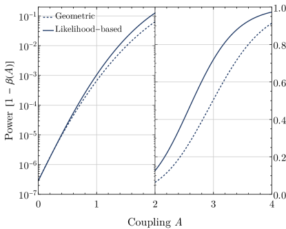
Figure 3: Power as a function of the coupling $A$. Dashed line: power for the geometric approach computed as in Equation (29). Solid line: power for the likelihood-based approach computed as in Equation (30). The values in the range $A\in[0,2]$ are magnified in logarithmic scale.

We proceed by comparing the power of both approaches; that is, the probability to correctly rejecting the null hypothesis, $H_{0}$ in (3), when the alternative hypothesis, $H_{1}$ is true. In other words, the power corresponds to the sensitivity of our test in detecting an axion expressed in probabilistic terms. In statistical literature, it is conventionally denoted as $1-\beta$, were $\beta$ corresponds to the probability of type II error, i.e., the probability of failing to reject $H_{0}$ when $H_{1}$ is true. In our case, the power is a function of the coupling $A$ constant and, for both the geometric and the likelihood-based rescan approach, it can be easily computed analytically. Specifically, for the geometric test, since $u_{\ell}=1$, for all $\ell=1,\dots,k_{\alpha}$, we have

$$1-\beta(A)=\left[1-\Phi(x_{\mathrm{thr}}-A)\right]^{k_{\alpha}-1};$$ (29)

whereas, the power of the likelihood-based rescan protocol is

$$1-\beta(A)=\sum_{h=1}^{k_{\alpha}}P(D_{h}|\,A).$$ (30)

In (30), the probabilities $P(D_{h}|\,A)$ can be calculated similarly to $P(D_{h}|\,H_{0})$ in (25). The power functions in (29) and (30) are plotted in Figure 3.

As expected, since the likelihood-based protocol uses more information, it also exhibits higher power; especially for larger values of the coupling constant, $A$. The two methods perform similarly when $A$ approaches zero.

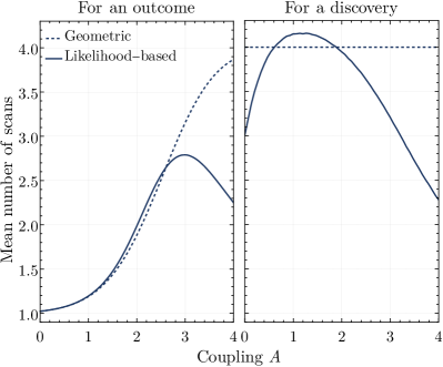
Figure 4: Mean number of scans needed to claim a statistical discovery (right) and to get an outcome, either a discovery or a no-discovery claim (left) for the two analysis approaches (Sections 3.1 and 3.2), for different values of the coupling $A$. The setup of the simulation is discussed in Section 3.3.

We emphasize once more that this is a toy example used for illustrative purposes but with no realistic physical meaning. In general, the value of $A$ is an alias for the coupling constant for the interaction channel under consideration and can carry units (see e.g. Section 5). For the same reason, the reachable sensitivity depends on the explicit values of $u_{\ell}$ (6), which can be constructed by tailoring the explicit configuration of a given detector. A fine tuning of the thresholds $x_{\mathrm{thr}}$ is also possible, in order to increase the power for smaller values of $A$. In this sense, analytic expressions (29) and (30) can be used to identify optimal choices of these parameters based on the specifics of the experiment being conducted.

Another useful aspect of the likelihood-based rescan protocol is that it does not require to perform all the $k_{\alpha}$ scans in order to claim a statistical discovery. Hence, it has the potential to reduce substantially the costs associated with additional rescans. Specifically, while a discovery claim via the geometric approach always requires us to perform $k_{\alpha}-1$ scans (see Figure 1), on average, we may expect the average number of scans required for a statistical discovery to be approximately the same or lower for the likelihood-based rescan protocol. This is illustrated on the right panel of Figure 4 by means of a Monte Carlo simulation for our toy example. The left panel, shows that the average number of scans required to reach a conclusion (either a discovery or a no-discovery claim) is lowered when relying of the likelihood-based rescan protocol for large values of the coupling. Whereas, given the initial tuning, it is the same for both frameworks as $A\to 0$.

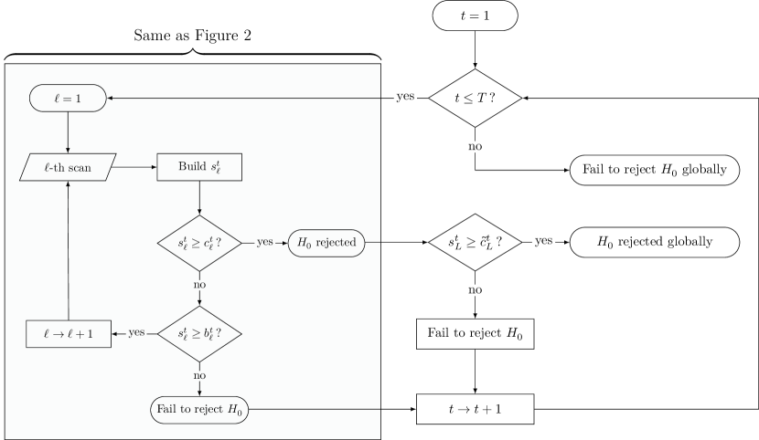
Figure 5: Flowchart of the likelihood-based rescan protocol (Figure 2) corrected to account for the scan of multiple frequencies.

4.   Look-elsewhere effect corrections

The protocols discussed in Section 3 can be meaningfully applied with no further modifications only when the interest is in testing only one given frequency. In the more realistic scenario where a set of $T\leq M$ frequencies $\{\nu_{t}\}_{t=1}^{T}$ is considered, the significance must be adjusted to account for the so-called look-elsewhere effect (LEE). That is, the probability that a random fluctuation may cross the discovery threshold anywhere over the frequency range considered. In other words, one must ensure that the probability of a false discovery at any frequency $\nu_{1},\,\dots,\,\nu_{T}$ does not exceed the desired significance level $\alpha$.

While several solutions to address the LEE have been proposed in literature [[, e.g.,]]Algeri:2016gtj,Foster:2017hbq, GV10, they are only applicable to the situation where just one scan is performed. In what follows, we discuss different approaches that allow us to correct for the LEE even when the data are collected sequentially over multiple scans.

The simplest possible solution is that of re-adapting classical approaches such as Šidák’s and Bonferroni corrections [[, e.g.,]]Algeri:2016gtj to our context. This can be done by replacing $\alpha$ in (18) with $1-(1-\alpha)^{1/T}$ for Šidák and with $\alpha/T$ for Bonferroni. The former provides an exact result, but relies on the assumption that all the test being performed are independent. Whereas, the latter trades the assumptions of independence for a much more conservative result, and, consequently, lower power.

Unfortunately, in axion searches, the $T$ tested frequencies are not independent. That is because the location of the axion is unknown, and thus, the step at which the frequency range is scanned is usually smaller than the expected width of the signal. This is done to ensure that no power is shared between two regions and thus dampened. Nonetheless, one can overcome this limitation by implementing Šidák or Bonferroni corrections based on the effective number of independent regions, $R_{T}^{\alpha}$. The latter can be defined as the value of independent tests that would determine the correct significance when replacing $\alpha$ in (18) with $R_{T}^{\alpha}$ (19) to compute the corresponding constants. Therefore, for a given value of $R_{T}^{\alpha}$, an adequate LEE correction can be obtained by replacing the probability of a discovery claim under $H_{0}$ at the $\ell$-th scan in (19) with

$$P(D_{t\ell}|\,H_{0})=1-\Bigl{(}1-\frac{\alpha}{k_{\alpha}}\Bigl{)}^{\nicefrac{{1}}{{R_{T}^{\alpha}}}}\approx\frac{\alpha}{R_{T}^{\alpha}k_{\alpha}}$$ (31)

in order to have

$$\sum_{t=1}^{T}\sum_{\ell=1}^{k_{\alpha}}P\left(D_{t\ell}\middle|\,H_{0}\right)=\alpha$$ (32)

for each of the frequencies, $t=1,\,\dots,\,T$, being tested. Hereinafter, we will refer to this framework as the independent regions approach. In the latter, the number of independent regions, $R_{T}^{\alpha}$, depends on both the number of scanned frequencies, $T$, and the significance level, $\alpha$. Therefore, the procedure requires a Monte Carlo calibration of $R_{T}^{\alpha}$ on the basis of (32) — see e.g. [27].

Here, we propose an alternative solution that allows us to overcome all the limitations of the above-mentioned approaches. Our strategy consists of constructing an updated version of the constants $c_{\ell}$ that accounts for the LEE, while leaving the likelihood-rescan protocol (Figure 2) at each of the $T$ frequencies unchanged. This can be done following the scheme on Figure 5; the main steps are described below.

For a given frequency, $t$, let $L_{t}$ be the scan at which an outcome is reached when following the rescan-protocol in Section 3.2 and Figure 2. Denote with $s_{L}^{t}$ the value of the test statistic at such scan; to ease the notation, the subscript $t$ has been dropped from $L_{t}$ since the dependency on frequency is reminded by the superscript. To control for the look-elsewhere effect we must guarantee that

$$P\left(\bigcup_{t=1}^{T}\left\{s_{L}^{t}-c_{L}^{t}\geq 0\right\}\middle|H_{0}\right)\leq\alpha,$$ (33)

which is equivalent to the condition

$$P\left(\max_{t=1,\dots,T}\left\{s_{L}^{t}-c_{L}^{t}\right\}>0\middle|H_{0}\right)\leq\alpha.$$ (34)

This leads to the definition of the new (global) statistic

$$\mathcal{S}=\max_{t=1,\dots,T}\left\{s_{L}^{t}-c_{L}^{t}\right\}.$$ (35)

which is simply the maximum of the stochastic process $\left\{s_{L}^{t}-c_{L}^{t}\right\}_{t=1}^{T}$. Notice that, while each $s_{\ell}$ in (14) is Gaussian, $s^{t}_{L}$ is not; that is because its distribution depends on the (binary) outcome of the decision rule in (15), and thus the value $L_{t}$ at which the decision is reached is itself random. Unfortunately, the distribution of $\mathcal{S}$ cannot be easily derived explicitly, nor it can be approximated using the upcrossings/Euler characteristic heuristic typically used in the context of LEE corrections [39, 40]. Nonetheless, it is possible to retrieve the null distribution of $\mathcal{S}$ by means of a Monte Carlo simulation.

Specifically, we are interested in estimating the quantile of order $1-\alpha$ of $\mathcal{S}$, i.e. $\mathcal{S}_{1-\alpha}$ for which

$$P(\mathcal{S}>\mathcal{S}_{1-\alpha})=\alpha.$$

We can then construct our newly “LEE-updated” constants, namely $\tilde{c}_{L}^{t}$, as

$$\tilde{c}_{L}^{t}=c_{L}^{t}+\mathcal{S}_{1-\alpha}.$$ (36)

Finally, a statistical discovery at (global) $\alpha$ significance is claimed if $s_{L}^{t}\geq\tilde{c}_{L}^{t}$ for at least one frequency $t=1,\,\dots,\,T$. The main steps of this approach are summarized in Figure 5.

Figure 6: Scheme of the setup assumed in the toy example of Section 4.1.

4.1.   Statistical properties of different LEE corrections

In this section, we investigate the properties of the look-elsewhere corrections described above by extending the toy example introduced in Section 3.3 to allow an analysis over multiple frequencies. Specifically, we start once again by considering a $5\sigma$ significance level ($\alpha=2.87\times 10^{-7}$) and $k_{\alpha}=5$, so that the constants $b_{\ell}$ and $c_{\ell}$ are those reported in Table 1. The setup considered is illustrated in Figure 6, and is intended to emulate as closely as possible a real axion experiment.

The data consist of a string of noise fluctuations $y_{i\ell}$, with the index $i$ marking the frequency $\nu_{i}$ at which the datum is taken; the subscript $\ell=1,\,\dots,\,k_{\alpha}$ indexes the rescan. For simplicity, we consider only one detector configuration, i.e., $N_{i}=1$ for all $i=1,\,\dots,\,M$, and thus the subscript $j$ is dropped.

We assume that $y_{i}\sim\mathcal{N}(\mu_{i}=0,\sigma_{i}=1)$, under $H_{0}$. Whereas, the alternative hypothesis, $H_{1}$, corresponds to a signal $\mu_{i}=A$, spanning over the neighborhood $\mathcal{I}_{\ell}^{t}$ of $\nu_{t}$. The latter consists of a row of $d=5$ frequency bins centered around $\nu_{t}$. For each frequency $\nu_{t}$, $t=1,\,\dots,\,T$, being tested, the respective set of fluctuations $Y_{\ell}^{t}$ is collected over $\mathcal{I}_{\ell}^{t}$. The quantities $x_{\ell}^{t}=\sum_{i=t-2}^{t+2}y_{i\ell}$ are then computed; whereas, the variances $u_{\ell}^{t}$ are constant and equal to $1/5$ for each $t=1,\dots,T$ and $\ell=1,\dots,k_{\alpha}$. Once an outcome is reached, $\nu_{t}$ is shifted by one bin and the procedure is repeated. Notice, once again, that $Y_{\ell}^{t}\cap Y_{\ell}^{t+1}\neq\varnothing$, thus the corresponding $x_{\ell}^{t}$ and $x_{\ell}^{t+1}$ (and the respective tests) are not independent.

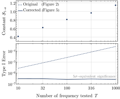
Figure 7: Top: Quantile of order $1-\alpha$ of the test statistic $\mathcal{S}$ in (35), as a function of the different number of frequencies $T$ tested. Bottom: Probabilities of false discoveries for the proposed LEE corrections based on (36) (solid line) and those obtained when conducting only a localized analyses at each individual frequency with no LEE correction (dashed line).

We implement the LEE corrections based on (36) where the quantile $\mathcal{S}_{1-\alpha}$ is estimated by means of a Monte Carlo simulation. The results obtained considering an increasing number of total frequencies, $T$, being tested are shown in the upper panel of Figure 7.

The bottom panel of Figure 7 shows that the LEE corrections based on (36) (solid line) ensure that the probability of false discovery is equal to the predetermined $5\sigma$ significance level. The same is not true when ignoring the LEE and conducting a local analysis at each individual frequency (dashed line). In this case, the probability of a false discovery increases with the number of tested frequencies.

For the sake of comparison, we also implement the LEE corrections based on the number of independent regions $R_{T}^{\alpha}$ (see Equation (31)). In this case, it is necessary to “tune” $R_{T}^{\alpha}$ by means of a Monte Carlo simulation. Figure 8, shows the probability of false discovery obtained when testing $T=100$ frequencies. Recall that, in this case, the analytical framework is the same as that in Figure 2 with the constants $c_{\ell}$ and $b_{\ell}$ computed by assuming different values of $R_{T}^{\alpha}$ in order to ensure the validity of (31). On the left panel of Figure 8, we consider a significance level of $3\sigma$, while the right panel corresponds to $5\sigma$. When choosing $R_{T}^{\alpha}=T=100$ the result is conservative (sensitivity loss); whereas, as $R_{T}^{\alpha}$ decreases the more we are susceptible to noise-triggered false claim. A linear fit applied to the Monte Carlo output shows that the number of independent region is $R_{100}^{5\sigma}\approx 98.3$ for a $5\sigma$ significance while it is sensibly lower in the $3\sigma$ case: $R_{100}^{3\sigma}\approx 86.2$.

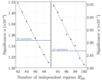
Figure 8: Probability of false discovery evaluated via Monte Carlo, when testing $T=100$ frequencies at $3\sigma$ equivalent significance (left) and $5\sigma$ (right), as a function of independent regions $R_{100}^{\alpha}$ considered.

Figure 9 compares the power of the LEE corrections based on (36) and those based on the independent regions approach at $3\sigma$ significance. Among the two, the independent region approach clearly enjoys higher power. This may be due to different reasons. Firstly, the procedure based on the independent regions lacks of what we may call “dangling outcomes”. That is, in the LEE framework of Figure 5, we may encounter the situation where

$$c_{L}^{t}\leq s_{L}^{t}<\tilde{c}_{L}^{t}.$$ (37)

In this case, the procedure stops and no discovery is claimed, even if the tested frequency has not been ruled out as a promising candidate. In fact, if only $s_{L}^{t}$ had fluctuated below $c_{L}^{t}$ (and $L<k_{\alpha}$) further scans would have been performed. Clearly, we may expect condition (37) to be in the “gray zone” between a very weak and very strong coupling. If $A\to 0$, we expect $s_{\ell}^{t}<b_{\ell}^{t}<c_{\ell}^{t}$ most of the times; whereas, if $A\to\infty$, we expect $s_{L}^{t}\gg\tilde{c}_{L}^{t}$.

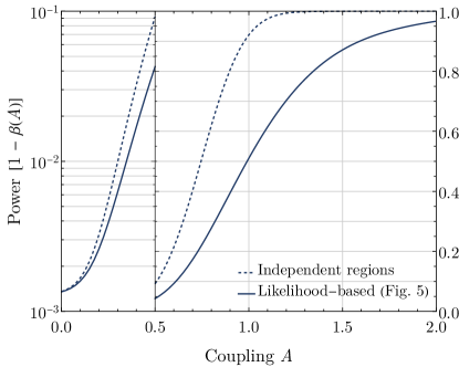
Figure 9: Power as a function of the coupling $A$ for a significance of $3\sigma$. Solid line: Corrected likelihood-based approach (Figure 5). Dashed line: likelihood-based approach (Figure 2) with $R_{100}^{3\sigma}\approx 86.2$ independent regions — see (31). The values in the range $A\in[0,\,0.5]$ are magnified in logarithmic scale.

As highlighted in Figure 10, the higher power reached by the independent-region procedure is also due to its tendency to perform more scans. In terms of number of scans needed, a peak is achieved in the transition between low to high powers (see e.g. left panel of Figure 10). The maximum difference in the number of scans per outcome occurs at approximately $A=1$ and corresponds to the highest relative difference between the two powers. In other words, the power increases with the number of performed scans, which is not surprising.

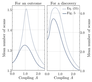
Figure 10: Mean number of scans needed to claim a statistical discovery (right) and to get an outcome, either a discovery or a no-discovery claim (left) for the approach outlined in Figure 5 (solid) and the one based on the application of the independent regions (dashed), for different values of the coupling $A$.

Everything highlighted so far applies to the case of a toy example. In a real experiment, the inferential procedure adopted needs to be tailored on the specific setup to which it is applied. Moreover, the performance of different approaches is bounded by practical constraints such as measurement time, sensitivity reach, or tuning. A direct comparison among them is hard to establish, since in a real setup not all scans are equal (like the $y_{i\ell}$ in the toy example) and the precision of each the measurement grows with the time invested in collecting the data. For instance, a procedure that is less sensitive but, on average, requires less scans to reach a conclusion (discovery/no discovery) allows researchers to redistribute the “extra time” to make fewer, but more precise, measurements. On this note, a procedure that reduces, at least on average, the number of scans needed is expected to be particularly impactful in view of future axion detectors, such as ALPHA [36], where the projected number of frequencies to be tested is on the order of $10^{7}$.

Finally, the CPU time required by each procedure is also non-negligible in practical applications. In this respect, calibrating the number of independent-regions, $R_{T}^{\alpha}$, via Monte Carlo, requires approximately one order of magnitude more of CPU time than estimating the quantile $\mathcal{S}_{1-\alpha}$ in (36). For instance, in our example, computing each point in Figure 8 takes the same amount of time needed to estimate $\mathcal{S}_{1-\alpha}$. Although not relevant in terms of statistical properties, the computational complexity may become a decisive factor when dealing with real data.

For all the above-mentioned reasons, what represents “the best strategy” strictly depends on the experimental conditions as well as on the time and computational resources available. In light of this, the development of a solution which is optimal with respect to both the number of rescans and the CPU time, while adjusting for the LEE, is left for future work.

5.   Application on upper limits

A straightforward application of the proposed framework to a real detector is when setting upper limits, i.e., the case when no significant signal is detected and thus, the outcome of the experiment is the exclusion of the couplings that would have likely generated a signal. This application is particularly useful when dealing when projecting the reach of future experiments, for which no data has yet to be produced. To ease the intuition, let’s consider once again the one scan-only framework of Section 3. To account for the possibility that a signal with some coupling $A$ is present, the test statistic in (5) can be reformulated as

$$s(A)=\sqrt{u}\left(\frac{x}{u}-A\right)$$ (38)

and is distributed as a standard normal random variable. For a given observed value, $\hat{s}(A)$, of (38), the upper limit for the coupling, $A_{\text{{ul}}}$, is the value of $A$ that solves

$$\Phi\bigl{(}\hat{s}(A)\bigl{)}=\alpha_{\text{{ul}}},$$ (39)

with $\alpha_{\text{{ul}}}$ being desired significance at which we aim to set our upper limit (e.g., $\alpha_{\text{{ul}}}=0.1$ for a $90\%$ upper limit). Since $\Phi(\cdot)$ is the distribution of a standard Gaussian, Equation (39) can be easily inverted. The resulting upper limit for $A$ is then

$$A_{\text{{ul}}}=\frac{\hat{x}/\sqrt{u}-\Phi^{-1}(\alpha_{\text{{ul}}})}{\sqrt{u}}.$$ (40)

This result is similar to what already found in [27]. Equation (40) can be further simplified when dealing with projected values of $\hat{x}$ in view of future experiments rather than actual measured data. In this case, we expect to measure a null power excess ($\hat{x}=0$). This gives an analytical formula which is statistically justified and can be easily applied — see e.g. [36].

In the remaining of this section, we demonstrate the validity of Equation (40) by comparing the resulting upper limit with the outcome of an analysis based on actual data. We will refer to the first run of HAYSTAC detector as presented in Refs. [31, 32]. Although the detector has been updated and newer results have been produced since then — see e.g. [41] — Ref. [32] is sufficiently detailed, in terms of general properties and data acquisition, to produce meaningful results.

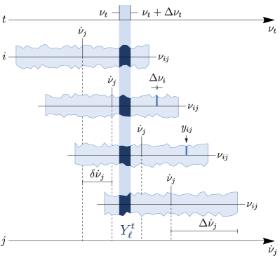
Figure 11: Sketch of the spectra, data format and relevant quantities for a HAYSTAC-like experiment.

Given its specifics, the experiment is designed to probe the frequency range $[5.7,\,5.8]\,$\mathrm{GHz}$$. The search is performed sequentially tuning the resonance of the cavity $\dot{\nu}_{j}$ at steps $\delta\dot{\nu}_{j}=$75\text{\,}\mathrm{kHz}$$. Following our notation, the subscript $j$ indexes the resonance of a given detector configuration and characterized by different values of its relevant parameters; for instance, the loaded quality factor $Q_{j}$ (see also Figure 5.13 of [32]).

At each configuration, the detector is sensitive to the range of frequencies $\nu_{ij}\in[\dot{\nu}_{j}-\dot{\nu}_{j}/Q_{j},\,\dot{\nu}_{j}+\dot{\nu}_{j}/Q_{j}]$; the latter correspond to the overlapping spectra in Figure 11. We denote with $\nu_{ij}$ the $i$-th frequency probed in the $j$-th configuration. Once a resonance is set, the power coming from a linear amplifier is measured for a total time $\tau_{j}=$15\text{\,}\min$$, and is averaged over the time $\tau_{ij}$ needed to reach the frequency resolution $\Delta\nu_{ij}=1/\tau_{ij}=$100\text{\,}\mathrm{Hz}$$. In the real data acquisition, the whole range is scanned twice, “followed by several shorter scans to compensate for nonuniform tuning” (see [32], Figure 6.7). In order to collect a reasonable amount of data for the following calculations, we rely on Section 4.3.5 of the same reference and assume that the frequency range has been scanned exactly $3$ times. In other words, each spectrum in Figure 11 comes in triplets or, conversely, we can imagine to deal with spectra acquired for $\tau_{j}=$45\text{\,}\min$$.

The averaged measured powers in each spectrum can be shifted and rescaled with respect to their mean baseline, leading to adimensional quantities (see for instance  Figure 2(c) in [35]). The resulting power fluctuations correspond to our $y_{ij}$ in Equation (1) and constitute the data sample used in our analysis (without any further scaling and/or rebinning). The standard deviation of each fluctuation $y_{ij}$ is

$$\sigma_{ij}=\sqrt{\frac{\tau_{ij}}{\tau_{j}}}=\frac{1}{\sqrt{\tau_{j}\Delta\nu_{ij}}}.$$ (41)

Whereas, their mean expresses the signal-to-noise ratio and can be factorized as (2). Here, $A$ is an alias of the physical coupling constant between an axion and two photons, i.e. $A=g_{a\gamma\gamma}^{2}$. Note that, in natural units, $g_{a\gamma\gamma}$ is usually expressed in ${\mathrm{eV}}^{-1}$. The factor $w_{ij}^{t}$ is nonzero only if the axion at frequency $t$ deposits power on the $i$-th bin of the $j$-th spectrum. Explicitly:

$$w_{ij}^{t}=\frac{P_{j}(\nu_{t})\,\sqrt{\tau_{ij}/\Delta\nu_{ij}}}{h\dot{\nu}_{j}\,N_{\mathrm{sys}}(\dot{\nu}_{j},\nu_{ij})}\,D(\nu_{t},\,\dot{\nu}_{j})\,L(\nu_{t},\,\nu_{ij}).$$ (42)

The parameterization of each term follows from Ref. [32]. Specifically, $P_{j}$ is the power per unit coupling constant (4.31), $N_{\mathrm{sys}}$ are the noise quanta (Figure 6.9 in [32]), $D(\nu_{t},\,\dot{\nu}_{j})$ as in Equation (5.2) of [32] accounts for the possible mismatch between $\dot{\nu}_{j}$ and $\nu_{t}$, while $L(\nu_{t},\,\nu_{ij})$ is the integral of the signal lineshape as in Equation (7.13) of [32] between each bin’s edges. That is, since $\Delta\nu_{t}=10^{-6}\nu_{t}\gg\Delta\nu_{ij}$, it quantifies the amount of signal falling in the bin.

Once the frequency $\nu_{t}$ to be tested has been selected, we can calculate the quantity $u^{t}$ in (6) by collecting the measurements obtained over the bins in the spectrum that falls within the range $\nu_{t}\leq\nu_{ij}\leq\nu_{t}+\Delta\nu_{t}$. We can then compute Equation (40) with $\hat{x}=0$ to obtain the projection of the 95% upper limit. The latter corresponds to the solid blue line in Figure 12. On the other hand, if we chose to define the upper limit with respect to the threshold value for a statistical discovery, $s_{5\sigma}=5$, we would end up with a result about a factor 1.45 higher, as shown in Figure 12 as dashed blue line. The definition of the upper limit in terms of a threshold value is the same as that adopted in Ref. [32]. Their result is also shown in Figure 12 as a gray curve. The results are quite compatible, even if our computation relies on many simplifications and parameterizations of time-dependent value describing the detector properties.

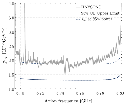
Figure 12: Upper limit projections for the first run of HAYSTAC detector originally presented in Refs. [31, 32] (gray line). Blue solid line line: 95% upper limit from Equation (40) with $\hat{x}=0$. Dashed line: limit given by $s_{5\sigma}=5$ at 95% power.

6.   Conclusions

In this paper, we have presented an inferential framework for axion searches that is statistically valid even when the experimental setup involves repeated scans. In Section 2, we have introduced the test statistic which is at the core of the likelihood-based rescan protocol discussed in Section 3.2 and is summarized in Figure 2. Specifically, when several scans are performed sequentially, our test statistic and the corresponding discovery thresholds are updated with as new sets of data are collected, until the fluctuation is reabsorbed or a statistical discovery is claimed. An important feature of the proposed procedure is that, when the analysis is performed at a fixed frequency, one can compute the power and the statistical significance analytically. Adequate comparisons with the so-called geometric approach have been conducted in Section 3.3 and have shown that the the likelihood-based inference enjoys higher power and, on average, a lower number of scans. Moreover, the likelihood-based inference provides a higher freedom in the definition of relevant quantities for data-acquisition. For instance, when the significance $\alpha$ and the maximum number of scans $k_{\alpha}$ have been set, the threshold $x_{\mathrm{thr}}$ in (13) is automatically determined and so is the rescan probability $p_{0}$. On the other hand, the likelihood-based approach allows for more freedom in specifying $p_{0}$ given $\alpha$ and $k_{\alpha}$ fixed, as one can tune the constants $b_{\ell}$ and $c_{\ell}$ in Equations (25)–(26) to achieve the desired significance.

Another important contribution of this work is the introduction of adequate corrections for look-elsewhere effect, and required when testing multiple axion frequencies $\nu_{t}$. Specifically, in Section 4, we have discussed Bonferroni and Sidak’s correction based on the effective number of independent regions, and we have introduced a novel alternative solution that is meant to ease the burden of the Monte Carlo tuning. The two approaches have been compared in Section 4.1 by means of a toy example. The latter has shown that, while the method based on the independent regions is characterized by a higher power, it is also requires, on average, a higher number of scans per outcome and discovery. It has to be noted, however, that establishing a direct comparison between the two in a real setup is a non-trivial task due to the interplay between the number of tested frequencies, the time spent measuring and the reachable precision of each measurement. An in-depth study of the performance of the different approaches when applied to real experiments is of paramount importance and paves the way to future improvements of this work.

Finally, in Section 5, we used our frequentist likelihood-based framework to reproduce a raw projection of the upper limit reachable by a realistic axion run in a real detector, as the phase one of HAYSTAC.

References

- [1] F. Zwicky “On the Masses of Nebulae and of Clusters of Nebulae” In Astrophys. J. 86, 1937, pp. 217–246 DOI: 10.1086/143864
- [2] L. Bergström “Nonbaryonic dark matter: Observational evidence and detection methods” In Rept. Prog. Phys. 63, 2000, pp. 793 DOI: 10.1088/0034-4885/63/5/2r3
- [3] G. Bertone, D. Hooper and J. Silk “Particle dark matter: Evidence, candidates and constraints” In Phys. Rept. 405, 2005, pp. 279–390 DOI: 10.1016/j.physrep.2004.08.031
- [4] J. Jaeckel and A. Ringwald “The Low-Energy Frontier of Particle Physics” In Ann. Rev. Nucl. Part. Sci. 60, 2010, pp. 405–437 DOI: 10.1146/annurev.nucl.012809.104433
- [5] J.. Feng “Dark Matter Candidates from Particle Physics and Methods of Detection” In Ann. Rev. Astron. Astrophys. 48, 2010, pp. 495–545 DOI: 10.1146/annurev-astro-082708-101659
- [6] S. Profumo, L. Giani and O.. Piattella “An Introduction to Particle Dark Matter” In Universe 5.10, 2019, pp. 213 DOI: 10.3390/universe5100213
- [7] A. Arbey and F. Mahmoudi “Dark matter and the early Universe: a review” In Prog. Part. Nucl. Phys. 119, 2021, pp. 103865 DOI: 10.1016/j.ppnp.2021.103865
- [8] D. Green “Snowmass Theory Frontier: Astrophysics and Cosmology”, 2022 arXiv:2209.06854 [hep-ph]
- [9] R.. Peccei and H.. Quinn “CP Conservation in the Presence of Instantons” In Phys. Rev. Lett. 38, 1977, pp. 1440–1443 DOI: 10.1103/PhysRevLett.38.1440
- [10] R.. Peccei and H.. Quinn “Constraints Imposed by CP Conservation in the Presence of Instantons” In Phys. Rev. D 16, 1977, pp. 1791–1797 DOI: 10.1103/PhysRevD.16.1791
- [11] S. Weinberg “A New Light Boson?” In Phys. Rev. Lett. 40, 1978, pp. 223–226 DOI: 10.1103/PhysRevLett.40.223
- [12] F. Wilczek “Problem of Strong and Invariance in the Presence of Instantons” In Phys. Rev. Lett. 40, 1978, pp. 279–282 DOI: 10.1103/PhysRevLett.40.279
- [13] J. Preskill, M.. Wise and F. Wilczek “Cosmology of the Invisible Axion” In Phys. Lett. B 120, 1983, pp. 127–132 DOI: 10.1016/0370-2693(83)90637-8
- [14] L.. Abbott and P. Sikivie “A Cosmological Bound on the Invisible Axion” In Phys. Lett. B 120, 1983, pp. 133–136 DOI: 10.1016/0370-2693(83)90638-X
- [15] M. Dine and W. Fischler “The Not So Harmless Axion” In Phys. Lett. B 120, 1983, pp. 137–141 DOI: 10.1016/0370-2693(83)90639-1
- [16] L. Di Luzio, M. Giannotti, E. Nardi and L. Visinelli “The landscape of QCD axion models” In Phys. Rept. 870, 2020, pp. 1–117 DOI: 10.1016/j.physrep.2020.06.002
- [17] K. Choi, S.. Im and C. Sub Shin “Recent Progress in the Physics of Axions and Axion-Like Particles” In Ann. Rev. Nucl. Part. Sci. 71, 2021, pp. 225–252 DOI: 10.1146/annurev-nucl-120720-031147
- [18] F. Chadha-Day, J. Ellis and D… Marsh “Axion dark matter: What is it and why now?” In Sci. Adv. 8.8, 2022, pp. abj3618 DOI: 10.1126/sciadv.abj3618
- [19] P.. Graham et al. “Experimental Searches for the Axion and Axion-Like Particles” In Ann. Rev. Nucl. Part. Sci. 65, 2015, pp. 485–514 DOI: 10.1146/annurev-nucl-102014-022120
- [20] I.. Irastorza and J. Redondo “New experimental approaches in the search for axion-like particles” In Prog. Part. Nucl. Phys. 102, 2018, pp. 89–159 DOI: 10.1016/j.ppnp.2018.05.003
- [21] J. Billard “Direct Detection of Dark Matter – APPEC Committee Report”, 2021 arXiv:2104.07634 [hep-ex]
- [22] I.. Irastorza “An introduction to axions and their detection” In SciPost Phys. Lect. Notes 45, 2022, pp. 1 DOI: 10.21468/SciPostPhysLectNotes.45
- [23] Y.. Semertzidis and S. Youn “Axion dark matter: How to see it?” In Sci. Adv. 8.8, 2022, pp. abm9928 DOI: 10.1126/sciadv.abm9928
- [24] C.. Adams “Axion Dark Matter” In 2022 Snowmass Summer Study, 2022 arXiv:2203.14923 [hep-ex]
- [25] P. Sikivie “Detection Rates for ’Invisible’ Axion Searches” [Erratum: Phys.Rev.D 36, 974 (1987)] In Phys. Rev. D 32, 1985, pp. 2988 DOI: 10.1103/PhysRevD.36.974
- [26] H. Primakoff “Photoproduction of neutral mesons in nuclear electric fields and the mean life of the neutral meson” In Phys. Rev. 81, 1951, pp. 899 DOI: 10.1103/PhysRev.81.899
- [27] J.. Foster, N.. Rodd and B.. Safdi “Revealing the Dark Matter Halo with Axion Direct Detection” In Phys. Rev. D 97.12, 2018, pp. 123006 DOI: 10.1103/PhysRevD.97.123006
- [28] S. Knirck et al. “Directional axion detection” In JCAP 11, 2018, pp. 051 DOI: 10.1088/1475-7516/2018/11/051
- [29] D.. Palken “Improved analysis framework for axion dark matter searches” In Phys. Rev. D 101.12, 2020, pp. 123011 DOI: 10.1103/PhysRevD.101.123011
- [30] S. Ahn et al. “Improved axion haloscope search analysis” In JHEP 04, 2021, pp. 297 DOI: 10.1007/JHEP04(2021)297
- [31] B.. Brubaker “First results from a microwave cavity axion search at 24 eV” In Phys. Rev. Lett. 118.6, 2017, pp. 061302 DOI: 10.1103/PhysRevLett.118.061302
- [32] B.. Brubaker “First results from the HAYSTAC axion search”, 2017 arXiv:1801.00835 [astro-ph.CO]
- [33] S.. Asztalos “Large scale microwave cavity search for dark matter axions” In Phys. Rev. D 64, 2001, pp. 092003 DOI: 10.1103/PhysRevD.64.092003
- [34] C. Bartram “Axion dark matter experiment: Run 1B analysis details” In Phys. Rev. D 103.3, 2021, pp. 032002 DOI: 10.1103/PhysRevD.103.032002
- [35] B.. Brubaker et al. “HAYSTAC axion search analysis procedure” In Phys. Rev. D 96.12, 2017, pp. 123008 DOI: 10.1103/PhysRevD.96.123008
- [36] A.. Millar “ALPHA: Searching For Dark Matter with Plasma Haloscopes”, 2022 arXiv:2210.00017 [hep-ph]
- [37] J.. Jensen “The modified signed likelihood statistic and saddlepoint approximations” In Biometrika 79.4 Oxford University Press, 1992, pp. 693–703
- [38] S. Algeri, J. Conrad, D.. Dyk and B. Anderson “On methods for correcting for the look-elsewhere effect in searches for new physics” In JINST 11.12, 2016, pp. P12010 DOI: 10.1088/1748-0221/11/12/P12010
- [39] E. Gross and O. Vitells “Trial factors for the look elsewhere effect in high energy physics” In The European Physical Journal C 70.1 Springer, 2010, pp. 525–530
- [40] S. Algeri and D.. Dyk “Testing One Hypothesis Multiple Times: The Multidimensional Case” In Journal of Computational and Graphical Statistics 29.2 Taylor & Francis, 2020, pp. 358–371
- [41] K.. Backes “A quantum-enhanced search for dark matter axions” In Nature 590.7845, 2021, pp. 238–242 DOI: 10.1038/s41586-021-03226-7