Oblique Quasi-Kink Modes in Solar Coronal Slabs Embedded in an Asymmetric Magnetic Environment: Resonant Damping, Phase and Group Diagrams

Abstract

There has been considerable interest in magnetoacoustic waves in static, straight, field-aligned, one-dimensional equilibria where the exteriors of a magnetic slab are different between the two sides. We focus on trapped, transverse fundamental, oblique quasi-kink modes in pressureless setups where the density varies continuously from a uniform interior (with density $\rho_{\rm i}$) to a uniform exterior on either side (with density $\rho_{\rm L}$ or $\rho_{\rm R}$), assuming $\rho_{\rm L}\leq\rho_{\rm R}\leq\rho_{\rm i}$. The continuous structuring and oblique propagation make our study new relative to pertinent studies, and lead to wave damping via the Alfv$\acute{\rm e}$n resonance. We compute resonantly damped quasi-kink modes as resistive eigenmodes, and isolate the effects of system asymmetry by varying $\rho_{\rm i}/\rho_{\rm R}$ from the “Fully Symmetric” ($\rho_{\rm i}/\rho_{\rm R}=\rho_{\rm i}/\rho_{\rm L}$) to the “Fully Asymmetric” limit ($\rho_{\rm i}/\rho_{\rm R}=1$). We find that the damping rates possess a nonmonotonic $\rho_{\rm i}/\rho_{\rm R}$-dependence as a result of the difference between the two Alfv$\acute{\rm e}$n continua, and resonant absorption occurs only in one continuum when $\rho_{\rm i}/\rho_{\rm R}$ is below some threshold. We also find that the system asymmetry results in two qualitatively different regimes for the phase and group diagrams. The phase and group trajectories lie essentially on the same side (different sides) relative to the equilibrium magnetic field when the configuration is not far from a “Fully Asymmetric” (“Fully Symmetric”) one. Our numerical results are understood by making analytical progress in the thin-boundary limit, and discussed for imaging observations of axial standing modes and impulsively excited wavetrains.

1 INTRODUCTION

It is well accepted that the highly structured solar atmosphere hosts a rich variety of low-frequency magnetohydrodynamic (MHD) waves and oscillations (see e.g., Jess et al., 2015; Khomenko & Collados, 2015; Li et al., 2020; Wang et al., 2021; Banerjee et al., 2021, for reviews). When observed, these waves/oscillations tend to be placed in the context of either atmospheric heating (see the reviews by e.g., De Moortel & Browning, 2015; Arregui, 2015; Van Doorsselaere et al., 2020) or solar atmospheric seismology (SAS, for reviews, see e.g., Nakariakov & Verwichte, 2005; De Moortel & Nakariakov, 2012; Nakariakov & Kolotkov, 2020). Whichever the context, a thorough theoretical understanding on MHD waves in structured media proves indispensable given the need to, say, pinpoint the physical identity of an observed oscillatory signal in the first place. Consequently, extensive use has long been made of equilibrium configurations where the physical parameters are structured only in one transverse direction, in both cylindrical (e.g., Rosenberg 1970; Zajtsev & Stepanov 1975; Wentzel 1979a; Edwin & Roberts 1983, hereafter ER83) and planar geometries (e.g., Ionson 1978; Wentzel 1979b; Roberts 1981a, b; Edwin & Roberts 1982, ER82 hereafter). While “a first approximation of reality” (Goossens et al., 2006, p.446), one-dimensional (1D) equilibria remain in routine use given the (semi-)analyitcal treatments they permit and/or the relevant wave physics they help elucidate.

Much progress has been made in the past two decades for cylindrical implementations of 1D equilibria. Let “ER83 equilibria” refer to the canonical, straight, field-aligned, static configurations addressed by ER83. Let “ER83-like equilibria” refer further to those that differ from the ER83 equilibria only by replacing the step transverse profiles therein with continuous ones. An extensive set of studies then indicated that the ER83 and/or ER83-like equilibria still yield new physics, to illustrate which point we name only a few examples. To start, revisiting kink modes in an ER83 equilibrium has enabled one to better understand both their physical nature (e.g., Goossens et al., 2009, 2012, 2014) and their energy-carrying capabilities (e.g., Goossens et al., 2013; Van Doorsselaere et al., 2014). Likewise, recent examinations on coronal sausage modes in either an ER83 (Vasheghani Farahani et al., 2014) or an ER83-like setup (e.g., Lopin & Nagorny, 2015; Yu et al., 2017) have shed new light on the wave behavior in the neighborhood of the critical axial wavenumbers that separate the trapped from the leaky regime. Furthermore, destructive interference has gained new attention (see Cally, 1991, and references therein for motivating ideas) as a unifying process that underlies the key notions of lateral leakage (e.g., Andries & Goossens, 2007; Oliver et al., 2015; Li et al., 2022), resonant damping, and phase mixing (Ruderman & Roberts 2002; Soler & Terradas 2015; also references therein). Note that these notions themselves are not specific to a particular mode, an example being the relevance of resonant damping to both kink and sausage modes (e.g., Giagkiozis et al., 2016; Goossens et al., 2021; Chen et al., 2021). Note also that new physics has also been gathered by considering those equilibria where the inhomogeneity can be rendered 1D by appropriate coordinate transformations but the configuration itself may differ considerably from ER83. The adoption of elliptic coordinates, for instance, yields a clear distinction between differently polarized kink modes in coronal loops with elliptic cross-sections (e.g., Ruderman 2003; Erdélyi & Morton 2009; also Morton & Ruderman 2011; Guo et al. 2020). Likewise, the application of bicylindrical coordinates to a system of two parallel loops enables one to address how a classic kink mode in an isolated loop splits into different kink-like oscillations that are polarized differently with respect to the orientation of the system (Van Doorsselaere et al. 2008; also Luna et al. 2008, 2009; Robertson et al. 2010), and how the resonant damping of these kink-like oscillations is affected by, say, the separation between the two loops (Robertson & Ruderman 2011; Gijsen & Van Doorsselaere 2014; see also Soler & Luna 2015).

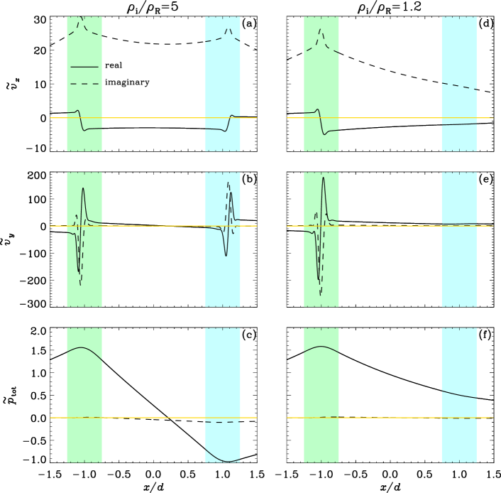
Figure 4: Eigenfunctions of resonantly damped oblique quasi-kink modes in an asymmetric slab configuration. A fixed combination $[\rho_{\rm i}/\rho_{\rm L},l/d,k_{y}d,k_{z}d]=[10,0.5,0.5,\pi/50]$ is adopted, whereas two values are examined for $\rho_{\rm i}/\rho_{\rm R}$, one being $5$ (the left column) and the other being $1.2$ (right). The portions shaded green and blue correspond to the left and right transition layers, respectively. The magnetic Reynolds number $R_{\rm m}$ is taken to be $10^{5}$. Plotted from top to bottom are the Fourier amplitudes of the transverse speed ($\tilde{v}_{x}$), the out-of-plane speed ($\tilde{v}_{y}$), and the total pressure perturbation ($\tilde{p}_{\rm tot}$). The eigenfunctions are scaled such that $\tilde{p}_{\rm tot}=1$ at $x=-2d$, their real (imaginary) parts represented by the solid (dashed) curves.

Planar implementations of 1D equilibria have also proven to be fruitful. Let an “ER82 equilibrium” refer to the canonical slab configuration examined in ER82, and restrict ourselves to only two groups of studies where ER82 is taken as a prototype. The first group focuses on curved slabs, motivated either by vertically polarized kink modes in active region (AR) loops first imaged by TRACE (e.g., Wang & Solanki, 2004; Wang et al., 2008) or by the TRACE (e.g., Schrijver et al., 2002; Verwichte et al., 2004) and SDO/AIA observations (e.g., Jain et al., 2015; Allian et al., 2019) that the response of coronal arcades to neighboring eruptions may involve the entire arcade rather than only individual structures embedded therein. Let $\bm{B}_{0}$ denote the equilibrium magnetic field. Let $\phi$ be the coordinate along $\bm{B}_{0}$, and $r$ a transverse coordinate. The equilibria are 1D in that the equilibrium quantities depend only on $r$, the third ($y$-) direction being ignorable. Some new insights then arise for, say, fast modes even when the $y$-propagation is prohibited (the $y$-wavenumber $k_{y}=0$). As examples, it was found that the $r$-slopes of the equilibrium quantities are crucial in determining whether fast modes can be trapped (e.g., Verwichte et al., 2006a; Pascoe & Nakariakov, 2016), and wave leakage into the ambient may need to surmount an evanescent barrier (e.g., Brady & Arber, 2005; Verwichte et al., 2006b). If a non-vanishing $k_{y}$ is further considered, then fast modes were shown to possess mixed polarizations in that their velocity perturbations involve the components both in and out of the $r-\phi$ plane (Thackray & Jain 2017; Lopin 2022; also Rial et al. 2010; Hindman & Jain 2015). Additional insights were also obtained in connection with the Alfv$\acute{\rm e}$n continuum, two notable examples being that fast wave energy may be transferred to Alfv$\acute{\rm e}$nic motions in the ambient (Rial et al., 2013) and that a new fast mode, heavily damped spatially, may occur when one sees the frequency rather than wavenumber as real-valued in the relevant eigenvalue problem (EVP) (Hindman & Jain, 2018). Note that the clear distinction between kink and sausage modes in ER82 tends not to hold (e.g., Díaz et al., 2006, Figure 4), the reason largely being that the equilibrium quantities in the ambient are not symmetric about the curved slab. Evidently, this imperfect distinction is not specific to curved configurations, and has in fact been the focus of the second group of recent studies.

The 1D equilibria addressed in the second group are not far from ER82. Let $(x,y,z)$ denote a Cartesian coordinate system, and let the equilibrium magnetic field $\bm{B}_{0}$ be aligned with the $z$-axis. The 1D equilibria are now structured only in $x$, being invariant and infinitely extended in $y$. As in ER82, three uniform regions are discriminated, the internal one being a slab and the other two being its exteriors . Different from ER82, however, is that the environment is asymmetric, namely the equilibrium quantities in one exterior are different from those in the other. A considerable number of EVP studies were devoted to magnetoacoustic waves propagating in the $x-z$ plane, with the initial efforts addressing nonmagnetic (e.g., Allcock & Erdélyi, 2017, 2018) versus magnetic exteriors (e.g., Zsámberger et al., 2018). Further addressed are such effects as time-stationary flows in the interior (e.g., Barbulescu & Erdélyi, 2018; Zsámberger et al., 2022b) or exterior (Zsámberger et al., 2022a), and the construction of axial standing modes with propagating ones (e.g., Oxley et al., 2020a, b). While sometimes rather complicated, this series of 1D equilibria turns out to be tractable semi-analytically. It is just that in general the resulting dispersion relations (DRs) do not factorize into independent expressions that govern kink and sausage modes individually. Nonetheless, the spatial behavior of the eigenfunctions still allows such terms as quasi-kink and quasi-sausage modes to be proposed (e.g., Allcock & Erdélyi, 2017, Figure 3). Overall, this series of studies demonstrated that the differences from ER82 in terms of the dispersion properties tend to be observationally relevant for, say, magnetic bright points (Shukhobodskaia & Erdélyi, 2018), light bridges (Zsámberger & Erdélyi, 2021), and flanks of coronal mass ejections (CMEs, Barbulescu & Erdélyi 2018). Conversely, the seismological techniques based on, say, amplitude ratios and/or minimum perturbation shifts can be invoked to infer how significantly one exterior differs from the other, a proposal that was both conceptually outlined (e.g., Allcock & Erdélyi, 2018; Zsámberger & Erdélyi, 2022) and observationally applied (e.g., Barbulescu & Erdélyi, 2018; Allcock et al., 2019).

This study is intended to present an EVP study on trapped, oblique, quasi-kink modes in straight, field-aligned, coronal slabs embedded in an asymmetric environment, the focus being on how the relevant dispersion properties are affected by the differences in one exterior from the other. Zero-beta MHD will be adopted, to comply with which a uniform equilibrium magnetic field $\bm{B}_{0}$ is taken. The structuring is therefore solely in the equilibrium density $\rho_{0}(x)$, from which a uniform interior (with density $\rho_{\rm i}$) and two uniform exteriors (with densities $\rho_{\rm L}$ and $\rho_{\rm R}$) are identified. Note that the exteriors will be referred to as “left” and “right” for the ease of description, and hence the subscripts ${\rm L}$ and ${\rm R}$. By so doing, the asymmetry of the system is entirely encapsulated in the density asymmetry, namely the difference between $\rho_{\rm L}$ and $\rho_{\rm R}$. Our study is new in the following aspects. Firstly, we will simultaneously incorporate a continuous $\rho_{0}(x)$ and a non-vanishing out-of-plane wavenumber $k_{y}$, making it inevitable for quasi-kink modes to be damped by the Alfv$\acute{\rm e}$n resonance. The need to incorporate the two factors can be seen as natural. The density asymmetry, however, means that two regimes may be distinguished by whether the resonance occurs in only one Alfv$\acute{\rm e}$n continuum or in both continua. This distinction, in turn, may have observational implications for, say, vertically polarized kink modes. Secondly, we will address how the density asymmetry affects the phase and group diagrams of oblique quasi-kink modes. This aspect of dispersion properties has not been examined in the literature to our knowledge, but is of general importance for understanding the large-time behavior of the system in response to impulsive and localized exciters. As such, our theoretical examination is expected to be relevant for a rather broad range of wave observations in slab-like structures, two examples being Sunward-moving dark tadpoles in post-flare supra-arcades (Verwichte et al., 2005), and CME-induced cyclic transverse motions of streamer stalks (streamer waves; e.g., Chen et al. 2010; Kwon et al. 2013; Decraemer et al. 2020).

This manuscript is structured as follows. Section 2 formulates our EVP and details its numerical solution procedure. The thin-boundary limit is examined in Section 3, where we address the EVP (semi-)analytically such that our numerical results can be validated and better understood. Section 4 then focuses on the resonant damping of quasi-kink modes, with our results on the phase and group diagrams collected in Section 5. We summarize this study in Section 6.

2 Problem Formulation

2.1 Equilibrium and Overall Description

We adopt zero-beta MHD throughout, for which the primitive quantities are the mass density ($\rho$), velocity ($\bm{v}$), and magnetic field ($\bm{B}$). Let the equilibrium quantities be denoted by a subscript $0$, and consider only static equilibria ($\bm{v}_{0}=0$). Let $(x,y,z)$ denote a Cartesian coordinate system, and let the uniform equilibrium magnetic field be $z$-aligned ($\bm{B}_{0}=B_{0}\bm{e}_{z}$). We assume that the equilibrium density ($\rho_{0}$) depends only on $x$, following

$$\rho_{0}(x)=\left\{\begin{array}[]{ll}\rho_{\rm L},&x<-x_{\rm e},\\[5.69046pt] \dfrac{1}{2}\left[(\rho_{\rm i}+\rho_{\rm L})-(\rho_{\rm i}-\rho_{\rm L})\sin\dfrac{\pi(-x-d)}{l}\right],&-x_{\rm e}\leq x\leq-x_{\rm i},\\[5.69046pt] \rho_{\rm i},&-x_{\rm i}<x<x_{\rm i},\\[5.69046pt] \dfrac{1}{2}\left[(\rho_{\rm i}+\rho_{\rm R})-(\rho_{\rm i}-\rho_{\rm R})\sin\dfrac{\pi(x-d)}{l}\right],&x_{\rm i}\leq x\leq x_{\rm e},\\[5.69046pt] \rho_{\rm R},&x>x_{\rm e},\end{array}\right.$$ (1)

with

$$x_{\rm i}=d-l/2,\quad x_{\rm e}=d+l/2.$$ (2)

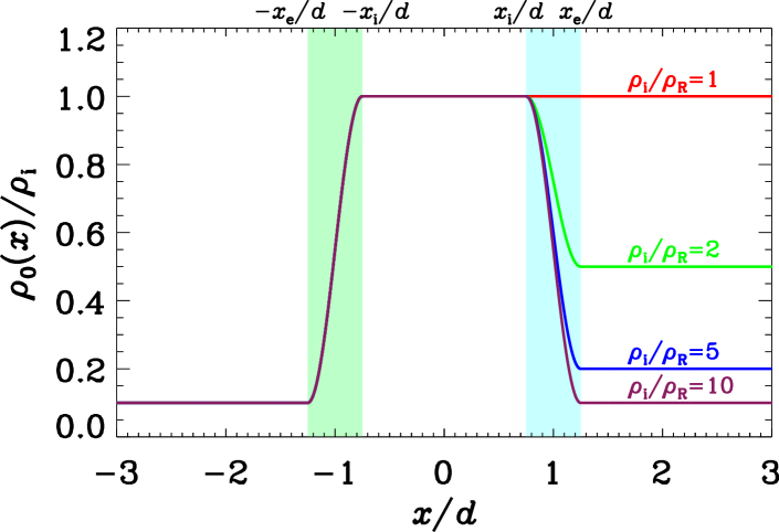
Figure 1: Transverse density profile $\rho_{0}(x)$ for the examined asymmetric slab system. Two transition layers (TLs, the shaded portions), centered around the nominal slab boundaries ($|x|=d$) and both of width $l$, are placed symmetrically about the nominal slab axis ($x=0$). Some smooth profile is adopted to connect the interior density $\rho_{\rm i}$ to $\rho_{\rm L}$ ($\rho_{\rm R}$), the density in the left (right) exterior (see Equation (1)). A pair $[\rho_{\rm i}/\rho_{\rm L},l/d]=[10,0.5]$ is adopted, while a number of $\rho_{\rm i}/\rho_{\rm R}$ are examined as labeled.

Here $d$ represents some nominal slab half-width, and $l$ the width of the two transition layers (TLs) that are geometrically symmetric about the nominal slab axis $x=0$. With subscript ${\rm i}$ we denote the equilibrium quantities in the interior. Likewise, the subscript ${\rm L}$ (${\rm R}$) refers to the equilibrium values in the left (right) exterior. The Alfv$\acute{\rm e}$n speed is defined via $v_{\rm A}^{2}(x)=B_{0}^{2}/\mu_{0}\rho_{0}(x)$ with $\mu_{0}$ being the magnetic permeability of free space. By $v_{\rm Ai}$ and $v_{\rm AL}$ ($v_{\rm AR}$) we then mean the Alfv$\acute{\rm e}$n speeds in the interior and left (right) exterior, respectively. Fixing $[\rho_{\rm i}/\rho_{\rm L},l/d]$ at $[10,0.5]$, Figure 1 plots $\rho_{0}$ against $x$ for several values of $\rho_{\rm i}/\rho_{\rm R}$ as labeled. Two extreme configurations are relevant and displayed, one corresponding to $\rho_{\rm R}=\rho_{\rm L}$ and the other to $\rho_{\rm R}=\rho_{\rm i}$. We consistently refer to the former (latter) as “Fully Symmetric” (“Fully Asymmetric”).

Oblique kink modes are in general resonantly absorbed in the Alfv$\acute{\rm e}$n continuum when the Alfv$\acute{\rm e}$n speed profiles are continuous (e.g., Section 8.14 in the textbook by Roberts, 2019), a well-established fact that holds here despite the notion “quasi-kink”. We proceed with a resistive eigenmode approach (see the review by Goossens et al. 2011, hereafter GER11, for conceptual clarifications). Let the subscript $1$ denote small-amplitude perturbations, which are governed by

$$\rho_{0}\dfrac{\partial\bm{v}_{1}}{\partial t} = \dfrac{(\nabla\times\bm{B}_{1})\times\bm{B}_{0}}{\mu_{0}},$$ (3)

$$\dfrac{\partial\bm{B}_{1}}{\partial t} = \nabla\times\left(\bm{v}_{1}\times\bm{B}_{0}-\dfrac{\eta}{\mu_{0}}\nabla\times\bm{B}_{1}\right).$$ (4)

Here $\eta$ denotes the Ohmic resistivity, assumed to be constant for simplicity. Any perturbation is Fourier-decomposed as

$$g_{1}(x,y,z;t)=\Re\{\tilde{g}(x)\exp[-i(\Omega t-k_{y}y-k_{z}z)]\},$$ (5)

with $\Omega$ being the complex-valued eigenfrequency, and $k_{z}$ ($k_{y}$) the real-valued axial (out-of-plane) wavenumber. Let $\omega$ ($\gamma$) denote the real (imaginary) part of $\Omega$. Only damping eigensolutions are of interest ($\gamma<0$). The equations that further govern the Fourier amplitudes $\tilde{v}_{x}$, $\tilde{v}_{y}$, $\tilde{B}_{x}$, $\tilde{B}_{y}$, and $\tilde{B}_{z}$ are identical to Equations (6) to (10) in Yu et al. (2021, hereafter Y21). As boundary conditions we require that all Fourier amplitudes vanish far from the slab, given that only trapped modes are of interest. Following Y21, we formulate and solve the resulting EVP with the finite-element code PDE2D (Sewell, 1988), which was first applied to solar contexts by Terradas et al. (2006) to our knowledge. We make sure that the details of the numerical setup, particularly where the boundaries are placed, do not influence our numerical solutions. The eigenfrequency $\Omega$ then formally writes

$$\dfrac{\Omega d}{v_{\rm Ai}}=\mathcal{F}\left(\dfrac{\rho_{\rm i}}{\rho_{\rm L}},\dfrac{\rho_{\rm i}}{\rho_{\rm R}},\dfrac{l}{d};k_{y}d,k_{z}d;R_{\rm m}\right),$$ (6)

where $R_{\rm m}=\mu_{0}v_{\rm Ai}d/\eta$ is some magnetic Reynolds number. Let asterisks denote complex conjugate. The following symmetry properties then follow from the governing equations. If $\Omega$ is an eigenfrequency for a given pair $[k_{y},k_{z}]$, then so is $-\Omega^{*}$. Furthermore, if $\Omega$ is an eigenfrequency for a given $[k_{y},k_{z}]$, then it remains an eigenfrequency for $[-k_{y},k_{z}]$, $[k_{y},-k_{z}]$, and $[-k_{y},-k_{z}]$. One is therefore allowed to assume $\omega>0$ and consider only the situation where $k_{y}\geq 0,k_{z}>0$.

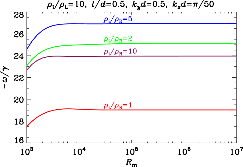
Figure 2: Dependencies of the damping efficiency on the magnetic Reynolds number $R_{\rm m}$ for oblique quasi-kink modes in asymmetric coronal slabs. The damping efficiency is measured by $\omega/|\gamma|$, with $\omega$ being the oscillation frequency and $\gamma$ the damping rate. A fixed combination $[\rho_{\rm i}/\rho_{\rm L},l/d,k_{y}d,k_{z}d]=[10,0.5,0.5,\pi/50]$ is adopted, whereas a number of values are examined for $\rho_{\rm i}/\rho_{\rm R}$ as labeled.

Resonantly damped modes stand out in that their eigenfrequencies become $R_{\rm m}$-independent for sufficiently large $R_{\rm m}$. This behavior was first shown by Poedts & Kerner (1991) in fusion contexts, and later demonstrated for an extensive set of solar configurations (e.g., Van Doorsselaere et al., 2004; Terradas et al., 2006; Guo et al., 2016; Chen et al., 2018, 2021). The same behavior is seen in Figure 2, where the ratios of the oscillation frequency to the damping rate ($\omega/|\gamma|$) are plotted against the magnetic Reynolds number $R_{\rm m}$ for a number of $\rho_{\rm i}/\rho_{\rm R}$ as labeled, with the combination $[\rho_{\rm i}/\rho_{\rm L},l/d,k_{y}d,k_{z}d]$ fixed at $[10,0.5,0.5,\pi/50]$. With Figure 2 as an example, we quote a typical value of $\sim 10^{4}-10^{5}$ for some critical $R_{\rm m}$ beyond which the eigenfrequencies remain constant. Only the $R_{\rm m}$-independent eigenfrequencies will be examined, meaning that

$$\dfrac{\Omega d}{v_{\rm Ai}}=\mathcal{F}\left(\dfrac{\rho_{\rm i}}{\rho_{\rm L}},\dfrac{\rho_{\rm i}}{\rho_{\rm R}},\dfrac{l}{d};k_{y}d,k_{z}d\right).$$ (7)

We further restrict ourselves, throughout this study, to those eigensolutions that are connected to the classic transverse fundamental kink mode arising in the situation where $\rho_{\rm L}=\rho_{\rm R}$, $l=0$ and $k_{y}=0$ (e.g., the textbook by Roberts, 2019, Figure 5.7). Evidently, the effects of density asymmetry can be brought out by seeing $\rho_{\rm i}/\rho_{\rm L}$ as fixed and examining those $\rho_{\rm i}/\rho_{\rm R}$ that are between the “Fully Symmetric” ($\rho_{\rm i}/\rho_{\rm R}=\rho_{\rm i}/\rho_{\rm L}$) and the “Fully Asymmetric” ($\rho_{\rm i}/\rho_{\rm R}=1$) limits. It then follows that the right Alfv$\acute{\rm e}$n continuum ($[k_{z}v_{\rm Ai},k_{z}v_{\rm AR}]$) is always enclosed by the left one ($[k_{z}v_{\rm Ai},k_{z}v_{\rm AL}]$). Note that the right resonance is necessarily irrelevant (relevant) for a “Fully Asymmetric” (“Fully Symmetric”) configuration. One therefore expects that the right resonance sets in only when $\rho_{\rm i}/\rho_{\rm R}$ exceeds some certain value when the rest of the parameters in the parentheses in Equation (7) are fixed. To ease our description, by $x^{\rm A}_{\rm L}$ and $x^{\rm A}_{\rm R}$ we consistently denote the locations of the left and right resonances even if the right resonance is absent. Regardless, we stress that the resonances are automatically handled by our resistive approach, and there is no need to consider the relevance of $x^{\rm A}_{\rm R}$ beforehand. We further remark that an eigenfrequency $\Omega$ is returned by the code together with the associated eigenfunctions, the latter being dependent on $R_{\rm m}$ despite the $R_{\rm m}$-independence of the former.

2.2 Energetics of Resonantly Damped Modes in Resistive MHD

It turns out to be necessary to examine the small-amplitude perturbations from the energetics perspective. We start by quoting a conservation law that follows from Equations (3) and (4) (see e.g., Braginskii, 1965; Leroy, 1985, for more general discussions),

$$\dfrac{\partial\epsilon}{\partial t}=-\nabla\cdot\bm{f}-s_{\rm res},$$ (8)

in which

$$\epsilon = \dfrac{1}{2}\rho_{0}\bm{v}_{1}^{2}+\dfrac{\bm{B}_{1}^{2}}{2\mu_{0}},$$ (9)

$$\bm{f} = p_{\rm tot}\bm{v}_{1}-\dfrac{1}{\mu_{0}}(\bm{v}_{1}\cdot\bm{B}_{1})\bm{B}_{0}+\dfrac{\eta}{\mu_{0}}\bm{j}_{1}\times\bm{B}_{1}$$ (10)

$$s_{\rm res} = \eta\bm{j}_{1}^{2}.$$ (11)

Here $p_{\rm tot}=\bm{B}_{0}\cdot\bm{B}_{1}/\mu_{0}$ is the Eulerian perturbation of total pressure, and $\bm{j}_{1}=\nabla\times\bm{B}_{1}/\mu_{0}$ is the perturbed electric current density. Evidently, $\epsilon$ represents the instantaneous wave energy density, $\bm{f}$ the Poynting vector, and $s_{\rm res}$ the Joule dissipation rate.

Suppose that a time-dependent system in question has settled to a resonantly damped eigenmode. Let $\bm{k}=k_{y}\bm{e}_{y}+k_{z}\bm{e}_{z}=k\bm{e}_{k}$ denote a 2D wavevector, with $k=|\bm{k}|$ and $\bm{e}_{k}=\bm{k}/k$. From $k$ we further define a wavelength $\lambda=2\pi/k$. One forms a right-handed coordinate system $(x,u_{\perp},u_{k})$ with $u_{k}$ being the coordinate in the $\bm{k}$-direction and $u_{\perp}$ the coordinate in the third direction. Now let $g_{1}$ and $h_{1}$ denote two arbitrary first-order quantities. It then follows from the Fourier ansatz (Equation (5)) that $g_{1}$ or $h_{1}$ depends on $y$ and $z$ only via the term $ku_{k}=k_{y}y+k_{z}z$. Consequently, the average of the second-order quantity $g_{1}h_{1}$ over one wavelength $\lambda$ reads

$$\left<g_{1}h_{1}\right>(x,t)\coloneqq\dfrac{1}{\lambda}\int_{0}^{\lambda}g_{1}(x,y,z,t)h_{1}(x,y,z,t){{\rm d}}u_{k}=\overline{g_{1}h_{1}}(x){\rm e}^{2\gamma t},$$ (12)

where

$$\overline{g_{1}h_{1}}(x)=\dfrac{1}{2}{\Re}[\tilde{g}^{*}(x)\tilde{h}(x)]=\dfrac{1}{2}{\Re}[\tilde{g}(x)\tilde{h}^{*}(x)].$$ (13)

We proceed with the well known fact that dissipative effects are important only in some dissipation layers (DLs) that embrace the resonances (see GER11 and references therein). Let $[x^{-}_{\rm L},x^{+}_{\rm L}]$ ($[x^{-}_{\rm R},x^{+}_{\rm R}]$) denote the left (right) DL. Consider a fixed volume $V$ that spans a length of $\lambda$ in the $\bm{k}$-direction and is of unit length in the $u_{\perp}$-direction. Furthermore, let its $x$-extent be the entire $x$-axis with the exception of the two DLs. Taking $\eta=0$ and integrating Equation (8) over $V$, one finds by repeatedly using Equation (12) that

$$-2\gamma\hat{E}=\hat{F}_{\rm L}+\hat{F}_{\rm R},$$ (14)

where

$$\begin{split}&\hat{E}=\left(\int_{-\infty}^{x^{-}_{\rm L}}+\int_{x^{+}_{\rm L}}^{x^{-}_{\rm R}}+\int_{x^{+}_{\rm R}}^{\infty}\right)\bar{\epsilon}(x){{\rm d}}x,\\ &\hat{F}_{\rm L}=\bar{f}_{x}(x^{-}_{\rm L})-\bar{f}_{x}(x^{+}_{\rm L}),\\ &\hat{F}_{\rm R}=\bar{f}_{x}(x^{-}_{\rm R})-\bar{f}_{x}(x^{+}_{\rm R}).\end{split}$$ (15)

Moreover, $f_{x}=p_{\rm tot}v_{1x}$ is the $x$-component of the Poynting vector. Technical details aside, Equation (14) reflects the simple fact that the wave energy in the ideal portions of the system is lost only via the net energy flux into the DLs where the Alfv$\acute{\rm e}$n resonances take place. It therefore follows that the contributions of individual resonances to the gross damping rate ($\gamma$) are measured by $\hat{F}_{\rm L}/2\hat{E}$ and $\hat{F}_{\rm R}/2\hat{E}$. Evidently, $\hat{F}_{\rm R}=0$ when the right resonance does not occur.

3 Oblique Quasi-kink Modes in the Thin-Boundary Limit

This section makes some analytical progress in the thin-boundary (TB) limit ($l/d\ll 1$) by capitalizing on the formulations for generic 1D equilibria (for first derivations, see e.g., Sakurai et al., 1991; Goossens et al., 1992; Ruderman et al., 1995; Tirry & Goossens, 1996). Our purposes are twofold. Firstly, we will derive the relevant dispersion relation (DR) such that its solutions can be employed to validate our resistive computations. We deem this validation necessary given that oblique quasi-kink modes have not been examined when the configuration does not take the “Fully Symmetric” or “Fully Asymmetric” limit. Secondly, we will collect some analytical expressions that approximately solve the DR for the two limiting configurations. This proves necessary not only for validation purposes but for understanding our numerical results on how the density asymmetry influences the phase and group diagrams.

3.1 General Formulations

We start by noting that the ideal version ($\eta=0$) of the governing equations can be combined to yield a well known equation for $\tilde{v}_{x}$ (e.g., Arregui et al. 2007; Y21; and references therein)

$$\left[\dfrac{k_{z}^{2}-\Omega^{2}/v_{\rm A}^{2}}{k_{y}^{2}+k_{z}^{2}-\Omega^{2}/v_{\rm A}^{2}}\tilde{v}_{x}^{\prime}\right]^{\prime}-\left(k_{z}^{2}-\Omega^{2}/v_{\rm A}^{2}\right)\tilde{v}_{x}=0,$$ (16)

where the shorthand notation ${}^{\prime}={\rm d}/{\rm d}x$ is employed. The Alfv$\acute{\rm e}$n resonance takes place wherever $\Omega=k_{z}v_{\rm A}$, and turns out to always (not necessarily) arise in the left (right) TL. Regardless, we consistently label the resonance(s) with the superscript ${\rm A}$, which is supplemented with the subscripts ${\rm L}$ or ${\rm R}$ when the left and right resonances need to be discriminated. We proceed by defining

$$\kappa_{j}^{2}=k_{z}^{2}-\dfrac{\Omega^{2}}{v_{{\rm A}j}^{2}},\quad m_{j}^{2}=k_{y}^{2}+\kappa_{j}^{2}=k_{y}^{2}+k_{z}^{2}-\dfrac{\Omega^{2}}{v_{{\rm A}j}^{2}},$$ (17)

where $j={\rm i,L,R}$ and we take $-\pi/2<\arg\kappa_{j},\arg m_{j}\leq\pi/2$ without loss of generality. The solution to Equation (16) in the uniform regions then writes

$$\tilde{v}_{x}(x)=\left\{\begin{array}[]{ll}A_{1}\exp(m_{\rm L}x),&x<-x_{\rm e},\\[2.84544pt] C_{1}\cosh(m_{\rm i}x)+C_{2}\sinh(m_{\rm i}x),&-x_{\rm i}<x<x_{\rm i},\\[2.84544pt] A_{2}\exp(-m_{\rm R}x),&x>x_{\rm e},\end{array}\right.$$ (18)

with $A_{1,2}$ and $C_{1,2}$ being constants. Likewise, the Fourier amplitude of the Eulerian perturbation of total pressure is given by

$$\tilde{p}_{\rm tot}=-\dfrac{i}{\Omega}\dfrac{B_{0}^{2}}{\mu_{0}}\times\left\{\begin{array}[]{ll}\dfrac{\kappa_{\rm L}^{2}}{m_{\rm L}}A_{1}\exp(m_{\rm L}x),&x<-x_{\rm e},\\[11.38092pt] \dfrac{\kappa_{\rm i}^{2}}{m_{\rm i}}\left[C_{1}\sinh(m_{\rm i}x)+C_{2}\cosh(m_{\rm i}x)\right],&-x_{\rm i}<x<x_{\rm i},\\[11.38092pt] -\dfrac{\kappa_{\rm R}^{2}}{m_{\rm R}}A_{2}\exp(-m_{\rm R}x),&x>x_{\rm e}.\end{array}\right.$$ (19)

The relevant DR in the TB limit is derived as follows. By construction, a DL where dissipative effects are important is thin, bracketing a resonance and bracketed by a TL (see e.g., GER11 for technical details). Let the variation of some quantity $q$ across a DL be denoted by $\llbracket q\rrbracket$, which is further taken by the TB treatment to be the variation of $q$ across the pertinent TL. The end result is that (e.g., Tirry & Goossens, 1996; Andries et al., 2000)

$$\begin{split}&\llbracket\tilde{p}_{\rm tot}\rrbracket=0,\\[5.69046pt] &\llbracket\tilde{\xi}_{x}\rrbracket=-\dfrac{i\pi k_{y}^{2}{\rm sgn}(\omega)}{\rho^{\rm A}|\Delta^{\rm A}|}\tilde{p}^{\rm A}_{\rm tot},\end{split}$$ (20)

where $\tilde{\xi}_{x}$ represents the Fourier amplitude of the transverse Lagrangian displacement defined via $\tilde{v}_{x}=-i\Omega\tilde{\xi}_{x}$. By the superscript ${\rm A}$ we mean that the relevant quantity is evaluated at a resonance ($x^{\rm A}_{\rm L}$ or $x^{\rm A}_{\rm R}$). In particular, $\Delta^{\rm A}$ is defined by (see Sakurai et al., 1991, where it was first introduced)

$$\Delta^{\rm A}=\left.\dfrac{{\rm d}(\omega^{2}-k_{z}^{2}v_{\rm A}^{2})}{{\rm d}x}\right|_{x=x^{\rm A}}.$$ (21)

A DR results when one connects the solutions in the uniform regions (Equations (18) and (19)) by the connection formulas (20), reading

$$\begin{split}&\left(\dfrac{\kappa_{\rm L}^{2}}{m_{\rm L}}\dfrac{\kappa_{\rm R}^{2}}{m_{\rm R}}+\dfrac{\kappa_{\rm i}^{4}}{m_{\rm i}^{2}}\right)+\left(\dfrac{\kappa_{\rm L}^{2}}{m_{\rm L}}+\dfrac{\kappa_{\rm R}^{2}}{m_{\rm R}}\right)\dfrac{\kappa_{\rm i}^{2}}{m_{\rm i}}\coth(2m_{\rm i}d)+\dfrac{\pi^{2}k_{y}^{4}}{k_{z}^{4}}\dfrac{\kappa_{\rm L}^{2}}{m_{\rm L}}\dfrac{\kappa_{\rm R}^{2}}{m_{\rm R}}\dfrac{\kappa_{\rm i}^{4}}{m_{\rm i}^{2}}\dfrac{\rho^{\rm A}_{\rm L}}{(\rho^{\prime})^{\rm A}_{\rm L}}\dfrac{\rho^{\rm A}_{\rm R}}{(\rho^{\prime})^{\rm A}_{\rm R}}\\[14.22636pt] &+\dfrac{i\pi k_{y}^{2}}{k_{z}^{2}}\dfrac{\kappa_{\rm L}^{2}}{m_{\rm L}}\dfrac{\kappa_{\rm R}^{2}}{m_{\rm R}}\dfrac{\kappa_{\rm i}^{2}}{m_{\rm i}}\left[\dfrac{\rho^{\rm A}_{\rm L}}{(\rho^{\prime})^{\rm A}_{\rm L}}-\dfrac{\rho^{\rm A}_{\rm R}}{(\rho^{\prime})^{\rm A}_{\rm R}}\right]\coth(2m_{\rm i}d)+\dfrac{i\pi k_{y}^{2}}{k_{z}^{2}}\dfrac{\kappa_{\rm i}^{4}}{m_{\rm i}^{2}}\left[\dfrac{\rho^{\rm A}_{\rm L}}{(\rho^{\prime})^{\rm A}_{\rm L}}\dfrac{\kappa_{\rm L}^{2}}{m_{\rm L}}-\dfrac{\rho^{\rm A}_{\rm R}}{(\rho^{\prime})^{\rm A}_{\rm R}}\dfrac{\kappa_{\rm R}^{2}}{m_{\rm R}}\right]=0,\end{split}$$ (22)

where $\rho$ actually means the equilibrium density $\rho_{0}$. Note that the identity $\rho_{0}(x)v_{\rm A}^{2}(x)={\rm const}$ in zero-beta MHD is employed to slightly simplify Equation (22). Note further that the right resonance is assumed to occur, as represented by the symbols $\rho^{\rm A}_{\rm R}$ and $(\rho^{\prime})^{\rm A}_{\rm R}$. We have additionally seen $\omega$ as positive, and employed the fact that $(\rho^{\prime})^{\rm A}_{\rm L}>0$ and $(\rho^{\prime})^{\rm A}_{\rm R}<0$ given our density profile (Equation (1)).

Some remarks are necessary here. Firstly, so far the examinations on quasi-kink modes in an asymmetric slab system pertain exclusively to the case where $k_{y}=0$ and $l=0$ (e.g., Allcock & Erdélyi, 2017; Zsámberger et al., 2018; Zsámberger & Erdélyi, 2020). Take the study by Zsámberger et al. (2018). The zero-beta version of Equation (16) therein writes

$$2(\kappa_{\rm i}^{2}+\kappa_{\rm L}\kappa_{\rm R})+\kappa_{\rm i}(\kappa_{\rm L}+\kappa_{\rm R})[\tanh(\kappa_{\rm i}d)+\coth(\kappa_{\rm i}d)]=0$$ (23)

with our notations. One readily verifies that Equation (23) is recovered by our Equation (22) when $k_{y}=0$. Generally speaking, neither Equation (22) nor Equation (23) can be factorized given the coupling between kink-like and sausage-like motions. Secondly, our discussions on Equation (7) indicate that the right resonance sets in only when $\rho_{\rm i}/\rho_{\rm R}$ exceeds some critical value $(\rho_{\rm i}/\rho_{\rm R})_{\rm crit}$. While assuming the relevance of the right resonance, Equation (22) can actually account for the situation where $\rho_{\rm i}/\rho_{\rm R}<(\rho_{\rm i}/\rho_{\rm R})_{\rm crit}$ by simply letting $\rho^{\rm A}_{\rm R}/(\rho^{\prime})^{\rm A}_{\rm R}=0$. One complication, however, is that in general we do not know when to switch off the $\rho^{\rm A}_{\rm R}/(\rho^{\prime})^{\rm A}_{\rm R}$ terms beforehand. Given our purposes, we choose to solve Equation (22) for only the two limiting cases ($\rho_{\rm i}/\rho_{\rm R}=\rho_{\rm i}/\rho_{\rm L}$ and $\rho_{\rm i}/\rho_{\rm R}=1$) plus one value of $\rho_{\rm i}/\rho_{\rm R}$ that lies in between. We discard the right resonance only when $\rho_{\rm i}/\rho_{\rm R}=1$. The range of $l/d$, on the other hand, is taken to be rather broad. Regardless, Equation (22) is always solved in an iterative manner. With a guess for $\Omega$, we determine the resonance location(s), evaluate the terms with a superscript ${\rm A}$, and then update $\Omega$ by a standard root-finder. This process is repeated until convergence. Note that the intermediate value of $\rho_{\rm i}/\rho_{\rm R}$ is chosen such that the right resonance arises for the entire range of $l/d$ to be examined. Note further that the full form of Equation (22) is solved for the two limiting cases, despite its simplifications in what follows.

3.2 “Fully Symmetric” and “Fully Asymmetric” Configurations

Consider first a “Fully Symmetric” configuration ($\rho_{\rm R}=\rho_{\rm L}$). It immediately follows from Equation (17) that $\kappa_{\rm L}=\kappa_{\rm R}$ and $m_{\rm L}=m_{\rm R}$. The right resonance is guaranteed, satisfying the relations $x^{\rm A}_{\rm R}=-x^{\rm A}_{\rm L}$, $\rho^{\rm A}_{\rm R}=\rho^{\rm A}_{\rm L}$, and $(\rho^{\prime})^{\rm A}_{\rm R}=-(\rho^{\prime})^{\rm A}_{\rm L}$. Defining

$$\alpha=\dfrac{\kappa_{\rm i}^{2}}{m_{\rm i}}\dfrac{m_{\rm L}}{\kappa_{\rm L}^{2}}-i\pi\dfrac{k_{y}^{2}}{k_{z}^{2}}\dfrac{\kappa_{\rm i}^{2}}{m_{\rm i}}\dfrac{\rho^{\rm A}_{\rm L}}{(\rho^{\prime})^{\rm A}_{\rm L}},$$ (24)

one finds that the left hand side (LHS) of Equation (22) can be factorized, the eigenfrequency $\Omega$ satisfying either $\coth(m_{\rm i}d)+\alpha=0$ or $\tanh(m_{\rm i}d)+\alpha=0$. The former is the DR for resonantly damped oblique kink modes , and more explicitly writes

$$\coth(m_{\rm i}d)=-\dfrac{\kappa_{\rm i}^{2}}{m_{\rm i}}\dfrac{m_{\rm L}}{\kappa_{\rm L}^{2}}+i\pi\dfrac{k_{y}^{2}}{k_{z}^{2}}\dfrac{\kappa_{\rm i}^{2}}{m_{\rm i}}\dfrac{\rho^{\rm A}_{\rm L}}{(\rho^{\prime})^{\rm A}_{\rm L}}.$$ (25)

The first derivation of Equation (25) with the resistive eigenmode approach was due to Goossens et al. (1992). Relevant here is the situation where $m_{\rm i}^{2}\approx m_{\rm L}^{2}\approx k_{y}^{2}$ and $|\gamma|\ll\omega$. Specializing to our density profile (Equation (1)), the approximate solution to Equation (25) can be summarized as

$$\omega^{2}\approx k_{z}^{2}v_{\rm Ai}^{2}\dfrac{1+\Theta}{\rho_{\rm L}/\rho_{\rm i}+\Theta},$$ (26)

$$\dfrac{\gamma}{\omega}\approx-\left(k_{y}l\right)\left(\dfrac{1+\Theta}{2\sqrt{\Theta}}\right)\left[\dfrac{(1-\rho_{\rm L}/\rho_{\rm i})\Theta^{2}}{(\rho_{\rm L}/\rho_{\rm i}+\Theta)(1+\Theta)^{2}}\right],$$ (27)

provided

$$k_{y}^{2}(\rho_{\rm L}/\rho_{\rm i}+\Theta)\gg k_{z}^{2}(1-\rho_{\rm L}/\rho_{\rm i}),\quad{\rm and}\quad|\gamma|\ll\omega.$$ (28)

Here $\Theta=\tanh(k_{y}d)$. Equations (26) and (27) were given in Y21, and a slightly different version was first derived for some different density profile by Tatsuno & Wakatani (1998) in fusion contexts. The first inequality in Equation (28) follows from the requirement $m_{\rm i}^{2}\approx m_{\rm L}^{2}\approx k_{y}^{2}$, and is derived here to make clearer the range of validity. The approximate solution simplifies considerably if one further assumes $k_{y}d\gg 1$ (namely $\Theta\approx 1$), a case that has been much-studied (e.g., Ionson, 1978; Goossens et al., 1992; Ruderman et al., 1995, to name only a few). In particular, Equation (26) becomes

$$\omega^{2}\approx k_{z}^{2}c_{\rm kL}^{2}=k_{z}^{2}\dfrac{2v_{\rm Ai}^{2}}{\rho_{\rm L}/\rho_{\rm i}+1},$$ (29)

with $c_{\rm kL}$ being the classic kink speed despite the cumbersome subscript ${\rm L}$.

Now move on to a “Fully Asymmetric” configuration ($\rho_{\rm R}=\rho_{\rm i}$), for which the right TL and hence the right resonance are absent. The relevant DR is actually also a special case of Equation (22), provided that one takes $\rho^{\rm A}_{\rm R}/(\rho^{\prime})^{\rm A}_{\rm R}=0$ and does not discriminate $\kappa_{\rm R}^{2}/m_{\rm R}$ from $\kappa_{\rm i}^{2}/m_{\rm i}$. Eliminating a common factor $1+\coth(2m_{\rm i}d)$, one finds that the DR writes

$$\dfrac{\kappa_{\rm L}^{2}}{m_{\rm L}}+\dfrac{\kappa_{\rm i}^{2}}{m_{\rm i}}+\dfrac{i\pi k_{y}^{2}}{k_{z}^{2}}\dfrac{\kappa_{\rm L}^{2}}{m_{\rm L}}\dfrac{\kappa_{\rm i}^{2}}{m_{\rm i}}\dfrac{\rho^{\rm A}_{\rm L}}{(\rho^{\prime})^{\rm A}_{\rm L}}=0,$$ (30)

where the cumbersome subscript ${\rm i}$ is retained instead of ${\rm R}$ to maintain formal consistency. Note that this configuration, pertinent to sheet pinch in fusion contexts, was the one that led to the concept of spatial resonance (Tataronis & Grossmann, 1973; Grossmann & Tataronis, 1973; Hasegawa & Chen, 1974; Chen & Hasegawa, 1974). There have been numerous solar applications of this configuration as well (e.g., Wentzel, 1979c; Lee & Roberts, 1986; Hollweg & Yang, 1988, to name only a few early studies), and the approximate expressions of interest ($m_{\rm i}^{2}\approx m_{\rm L}^{2}\approx k_{y}^{2}$, $|\gamma|\ll\omega$) can be collected as

$$\omega^{2}\approx k_{z}^{2}c_{\rm kL}^{2},$$ (31)

$$\dfrac{\gamma}{\omega}\approx-\dfrac{k_{y}l}{4}\dfrac{1-\rho_{\rm L}/\rho_{\rm i}}{1+\rho_{\rm L}/\rho_{\rm i}},$$ (32)

which holds for our density profile (Equation (1)) provided that

$$k_{y}^{2}(\rho_{\rm L}/\rho_{\rm i}+1)\gg k_{z}^{2}(1-\rho_{\rm L}/\rho_{\rm i}),\quad{\rm and}\quad|\gamma|\ll\omega.$$ (33)

Equations (31) and (32), together with their explicit range of validity (Equation (33)), are seen to agree with the $\Theta\approx 1$ limit of the “Fully Symmetric” results.

4 Results I: Rates of Resonant Absorption

This section examines the resonant damping of oblique quasi-kink modes, assuming that $k_{y}$ and $k_{z}$ can be observationally identified. Evidently, the parentheses in Equation (7) contain way too many parameters to exhaust. We choose a fixed $\rho_{\rm i}/\rho_{\rm L}=10$, a density contrast that is reasonable for say, AR loops (e.g., Aschwanden et al., 2004), polar plumes (e.g., Wilhelm et al., 2011), and streamer stalks (e.g., Chen et al., 2011). The dimensionless axial wavenumber $k_{z}d$ will be fixed at $\pi/50$, which is reasonable for axial fundamentals or their first several harmonics in coronal structures typically imaged in the EUV (e.g., Schrijver, 2007, Figure 1). We additionally restrict ourselves to the situation where $k_{y}>k_{z}$ (or even $k_{y}\gg k_{z}$), largely organizing our results around the role of $\rho_{\rm i}/\rho_{\rm R}$.

4.1 Validation of Resistive Computations Against Thin-Boundary Expectations

Figure 3 starts our examination by comparing the resistive results (labeled “Resis”, the black curves) with the relevant TB expectations (red and blue) for a fixed combination $[\rho_{\rm i}/\rho_{\rm L},k_{y}d,k_{z}d]=[10,0.5,\pi/50]$. Plotted are the oscillation frequency ($\omega$, the upper row) and the ratio of the damping rate to the oscillation frequency ($-\gamma/\omega$, lower) as functions of the dimensionless TL width ($l/d$). A number of values are examined for $\rho_{\rm i}/\rho_{\rm R}$ as discriminated by the line styles. Two groups of TB results are presented, one being the iterative solutions to Equaiton (22) (labeled “TB num”, the left column), and the other being those evaluated with the approximate analytical expressions (“TB analytic”, right). Note that only the “Fully Asymmetric” ($\rho_{\rm i}/\rho_{\rm R}=1$) and “Fully Symmetric” ($\rho_{\rm i}/\rho_{\rm R}=\rho_{\rm i}/\rho_{\rm L}$) cases are examined in the right column, given the limited availability of the analytical expressions (see Equations (26) and (27) as well as (31) and (32)). Consider the left column first. One immediately sees that the resistive results agree remarkably well with the “TB num” ones for, say, $l/d\lesssim 1$, meaning that the two independent approaches are both correctly implemented. Furthermore, there actually exists a rather close agreement between the two sets of solutions even for $l/d\sim 2$, the only exception being in the $-\gamma/\omega$ profile for $\rho_{\rm i}/\rho_{\rm R}=1$. Now move on to the right column, where one sees that the approximate expressions perform even better than the iterative solutions in reproducing the resistive results, despite that the iterative approach is more self-consistent in principle. Overall, Figure 3 offers yet another piece of evidence that the TB expectations for coronal equilibria may hold well beyond their nominal range of applicability (e.g., Van Doorsselaere et al., 2004; Soler et al., 2013; Chen et al., 2021). We conclude further that faith can be placed in our resistive approach, which will be consistently adopted hereafter. As for the TB approximation, we choose to invoke only the approximate expressions for the two limiting values of $\rho_{\rm i}/\rho_{\rm R}$ when necessary. The reasons for us to do this are largely twofold, one being the complication for assessing the relevance of the right resonance a priori, and the other being the general difficulty to further proceed analytically when $\rho_{\rm i}/\rho_{\rm R}$ is between the extreme values.

4.2 Effects of Density Asymmetry

Whether the right resonance occurs is most readily revealed by the spatial profiles of the resistive eigenfunctions, for which purpose Figure 4 plots the Fourier amplitudes of the transverse speed ($\tilde{v}_{x}$, the top row), the out-of-plane speed ($\tilde{v}_{y}$, middle), and the Eulerian perturbation of total pressure ($\tilde{p}_{\rm tot}$, bottom). Two values for $\rho_{\rm i}/\rho_{\rm R}$ are examined, one being $5$ (the left column) and the other being $1.2$ (right), whereas the combination $[\rho_{\rm i}/\rho_{\rm L},l/d,k_{y}d,k_{z}d]$ is fixed at $[10,0.5,0.5,\pi/50]$. We additionally take the magnetic Reynolds number $R_{\rm m}$ to be $10^{5}$ for both columns. The left and right TLs correspond to the portions shaded green and blue, respectively. Furthermore, the eigenfunctions are scaled such that $\tilde{p}_{\rm tot}$ attains unity at $x=-2d$, their real (imaginary) parts represented by the solid (dashed) curves. Now that ideal MHD essentially applies at $x=-2d$, our way for rescaling the eigenfunctions means that any Alfv$\acute{\rm e}$n resonance is characterized by the following features (see GER11 and references therein). The strongest dynamics occurs for $\tilde{v}_{y}$ given the so-called $1/s$ singularity, and the dynamics of $\Im\tilde{v}_{x}$ is the second strongest as a result of some $\ln s$ singularity. The total pressure perturbation $\tilde{p}_{\rm tot}$ possesses the least strong variation, which in fact cannot be discerned for the examined parameters. One therefore sees that the right resonance is relevant (irrelevant) when $\rho_{\rm i}/\rho_{\rm R}=5$ ($\rho_{\rm i}/\rho_{\rm R}=1.2$). With the left resonance for $\rho_{\rm i}/\rho_{\rm R}=5$ as an example, one further sees that $\Re\tilde{v}_{x}$ jumps at any resonance location (see e.g., Figure 4a), and $\tilde{p}_{\rm tot}$ is dominated by its real part there (e.g., Figure 4c). Given Equation (15), the sign of $\Re\tilde{p}_{\rm tot}$ and that of the jump in $\Re\tilde{v}_{x}$ then dictate that $\hat{F}$, the net energy flux into a resonance, is always positive. On top of that, an inspection of the magnitudes of $\Re\tilde{p}_{\rm tot}$ and the jump in $\Re\tilde{v}_{x}$ in the left column indicates that $\hat{F}_{\rm L}>\hat{F}_{\rm R}$, meaning that the left resonance plays a more important role in damping the oblique quasi-kink mode at hand.

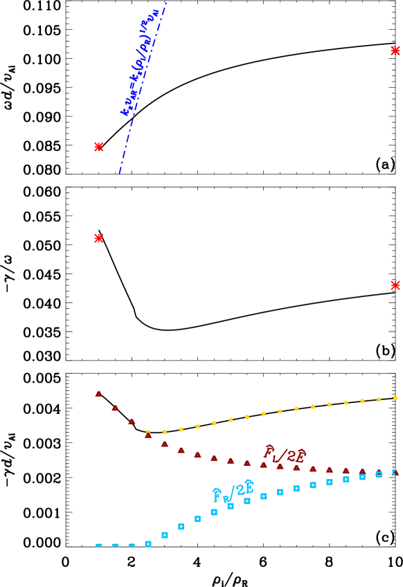
Figure 5: Effects of density asymmetry on resonantly damped oblique quasi-kink modes in an asymmetric slab configuration. Plotted are the dependencies on $\rho_{\rm i}/\rho_{\rm R}$ of (a) the oscillation frequency $\omega$, (b) the ratio of the damping rate to oscillation frequency $-\gamma/\omega$, and (c) the damping rate $-\gamma$. The combination $[\rho_{\rm i}/\rho_{\rm L},l/d,k_{y}d,k_{z}d]$ is fixed at $[10,0.5,0.5,\pi/50]$. The red asterisks in (a) and (b) are obtained with the approximate expressions for the “Fully Asymmetric” and “Fully Symmetric” configurations in the thin-boundary limit. Furthermore, the blue dash-dotted curve in (a) represents the upper end of the right Alfv$\acute{\rm e}$n continuum ($k_{z}v_{\rm AR}$). The open triangles (boxes) in (c) correspond to the contribution to the gross damping rate from the left (right) resonance, as evaluated with the relevant eigenfunctions. The sum of the individual contributions is further given by the filled circles. See text for more details.

We are now ready to examine somehow more systematically the influence of density asymmetry on the damping rates of resonantly damped quasi-kink modes. Fixing $[\rho_{\rm i}/\rho_{\rm L},l/d,k_{y}d,k_{z}d]$ at $[10,0.5,0.5,\pi/50]$, Figure 5 presents, by the solid curves, the $\rho_{\rm i}/\rho_{\rm R}$-dependencies of (a) the oscillation frequency $\omega$, (b) the ratio of the damping rate to oscillation frequency $-\gamma/\omega$, and (c) the damping rate $-\gamma$ itself. The asterisks in Figures 5a and 5b represent the TB expectations from the approximate expressions in the “Fully Asymmetric” and “Fully Symmetric” limits (Equations (26) and (27) as well as (31) and (32)). Note that these analytical results are presented largely for reference, given that Figure 3 has already shown that they are rather close to the resistive results. Now examine Figures 5a, where the dash-dotted curve represents the $\rho_{\rm i}/\rho_{\rm R}$-dependence of the upper bound of the right Alfv$\acute{\rm e}$n continuum ($k_{z}v_{\rm AR}$). One sees that the oscillation frequency $\omega$ tends to increase monotonically with $\rho_{\rm i}/\rho_{\rm R}$, which is intuitively understandable because the effective inertia of the system tends to diminish as the MHD fluid in the right exterior becomes increasingly rarefied. Nonetheless, $\omega$ possesses only a rather weak dependence on $\rho_{\rm i}/\rho_{\rm R}$, being readily overtaken by $k_{z}v_{\rm AR}=k_{z}v_{\rm Ai}\sqrt{\rho_{\rm i}/\rho_{\rm R}}$ at some critical $(\rho_{\rm i}/\rho_{\rm R})_{\rm crit}\approx 2.04$. Evidently, this $(\rho_{\rm i}/\rho_{\rm R})_{\rm crit}$ is where the right resonance starts to be relevant. It therefore comes as no surprise that this $(\rho_{\rm i}/\rho_{\rm R})_{\rm crit}$ is reflected in Figure 5b, where the sudden onset of the right resonance somehow leads to a break in the $-\gamma/\omega$ curve. Regardless, more important to note is that $-\gamma/\omega$ possesses an overall nonmonotic dependence on $\rho_{\rm i}/\rho_{\rm R}$, attaining some local minimum at $(\rho_{\rm i}/\rho_{\rm R})_{\rm min}\approx 3.09$. It is interesting to see that $(\rho_{\rm i}/\rho_{\rm R})_{\rm min}$ does not coincide with $(\rho_{\rm i}/\rho_{\rm R})_{\rm crit}$, namely the onset of the right resonance does not immediately enhance the gross damping efficiency. Intuitively speaking, one expects that the relative importance of the two resonances is responsible for both the overall nonmonotonic $\rho_{\rm i}/\rho_{\rm R}$-dependence of $-\gamma/\omega$ and the difference of $(\rho_{\rm i}/\rho_{\rm R})_{\rm min}$ from $(\rho_{\rm i}/\rho_{\rm R})_{\rm crit}$. In principle, this intuitive expectation can be readily examined given that the contribution of an individual resonance is measurable by $\hat{F}/2\hat{E}$ (see Equation (14)), and one can readily perceive how $\hat{F}_{\rm R}$ compares with $\hat{F}_{\rm L}$ (see the discussions on Figures 4a and 4c). In practice, however, there arises some difficulty to quantify $\hat{F}$ for a resonance due to the need to pinpoint the pertinent DL (see e.g., Chen et al., 2021, for details). We tackle this by following the empirical approach therein, performing two computations with $R_{\rm m}$ being $10^{6}$ and $2\times 10^{6}$, scaling the eigenfunctions in the same way as in Figure 4, and eventually deeming a DL to be where $|\tilde{v}_{x}|$ differs by a factor $\geq 2\times 10^{-4}$ between the two resistive solutions. Evaluating $\hat{F}_{\rm L}/2\hat{E}$ and $\hat{F}_{\rm R}/2\hat{E}$ with Equation (15), Figure 5c then plots their corresponding values by the open triangles and squares, respectively. Their sum is further presented by the filled circles. Two features then follow. Firstly, the indirectly evaluated damping rates, $(\hat{F}_{\rm L}+\hat{F}_{\rm R})/2\hat{E}$, agree remarkably well with those directly output from the code ($-\gamma$), as evidenced by that the filled circles are threaded by the solid curve. This further corroborates the remarkable accuracy of the resistive computations. Secondly, the contribution to the gross damping rate from the left resonance ($\hat{F}_{\rm L}/2\hat{E}$) decreases monotonically with $\rho_{\rm i}/\rho_{\rm R}$, thereby making it natural to see the decrease of $-\gamma/\omega$ when $\rho_{\rm i}/\rho_{\rm R}$ varies from unity to $(\rho_{\rm i}/\rho_{\rm R})_{\rm crit}$. The right contribution, on the other hand, increases monotonically when $\rho_{\rm i}/\rho_{\rm R}$ increases from $(\rho_{\rm i}/\rho_{\rm R})_{\rm crit}$, tending to the left contribution when the “Fully Symmetric” configuration is approached. After setting in, the right contribution nonetheless only partially offsets the reduction in the left contribution, and hence the difference between $(\rho_{\rm i}/\rho_{\rm R})_{\rm min}$ and $(\rho_{\rm i}/\rho_{\rm R})_{\rm crit}$.

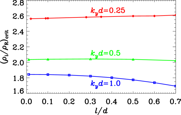
Figure 6: Dependencies on the dimensionless TL width ($l/d$) of the critical density contrast $(\rho_{\rm i}/\rho_{\rm R})_{\rm crit}$, only above which is the right Alfv$\acute{\rm e}$n resonance relevant. The combination $[\rho_{\rm i}/\rho_{\rm L},k_{z}d]$ is fixed at $[10,\pi/50]$, whereas a number of $k_{y}d$ are examined as labeled.

Guided by Equation (7), one may take Figure 5a as an approach for locating some specific $(\rho_{\rm i}/\rho_{\rm R})_{\rm crit}$ for a given combination $[\rho_{\rm i}/\rho_{\rm L},l/d,k_{y}d,k_{z}d]$. Figure 6 capitalizes on this approach to show $(\rho_{\rm i}/\rho_{\rm R})_{\rm crit}$ as a function of $l/d$ for a number of values of $k_{y}d$ when $[\rho_{\rm i}/\rho_{\rm L},k_{z}d]$ is fixed at $[10,\pi/50]$. In essence, any curve is a dividing line that separates the $\rho_{\rm i}/\rho_{\rm R}-l/d$ plane into two portions, the right resonance being absent (present) in the portion below (above). One sees that $(\rho_{\rm i}/\rho_{\rm R})_{\rm crit}$ for a given $k_{y}d$ possesses only a rather weak dependence on the dimensionless TL width ($l/d$), a behavior that evidently derives from the $l/d$-insensitivity of the oscillation frequency $\omega$ (see Figure 3a). For a given $l/d$, on the other hand, $(\rho_{\rm i}/\rho_{\rm R})_{\rm crit}$ is seen to possess some stronger dependence on $k_{y}d$. Evidently, this dependence follows from the fact that $\omega$ tends to decrease somehow appreciably when $k_{y}d$ increases in the examined range. These details aside, Figure 6 means that it makes sense to estimate the critical density contrast $(\rho_{\rm i}/\rho_{\rm R})_{\rm crit}$ by using the $l=0$ version of Equation (22), provided that the $l/d$-insensitivity of $\omega$ proves sufficiently general. This $l=0$ version can be readily implemented by retaining only the first two terms on the LHS of Equation (22), writing specifically

$$\left(\dfrac{\kappa_{\rm L}^{2}}{m_{\rm L}}\dfrac{\kappa_{\rm R}^{2}}{m_{\rm R}}+\dfrac{\kappa_{\rm i}^{4}}{m_{\rm i}^{2}}\right)+\left(\dfrac{\kappa_{\rm L}^{2}}{m_{\rm L}}+\dfrac{\kappa_{\rm R}^{2}}{m_{\rm R}}\right)\dfrac{\kappa_{\rm i}^{2}}{m_{\rm i}}\coth(2m_{\rm i}d)=0.$$ (34)

Note that $k_{y}$ remains involved via the terms $m_{\rm i}$, $m_{\rm L}$, and $m_{\rm R}$ (see Equation (17)). Note further that estimating $(\rho_{\rm i}/\rho_{\rm R})_{\rm crit}$ with Equation (34) is less time-consuming than the full resistive eigenmode approach. However, this does not mean that our resistive approach is not worth pursuing, for the $l/d$-insensitivity of $\omega$ is not known beforehand even for the parameters examined in Figure 6. On top of that, the resistive approach is actually easier to implement than the TB formulation (Equation (22)) when one is interested in, say, the damping rates.

4.3 Discussion

The observational implications of our results on resonant absorption may be illustrated by seeing our equilibrium configuration as a straightened version of the much-studied curved arcade system (e.g., Verwichte et al., 2006a; Thackray & Jain, 2017). Let our $x-z$ plane be identified as the plane of sky (PoS) for the ease of description. Likewise, let our configuration be bounded in the axial direction by two photospheres at $z=0$ and $z=L$, with $L$ being the arcade length. The left (right) exterior then actually corresponds to the outer (inner) ambient corona that overlies (underlies) the arcade given that $\rho_{\rm L}\leq\rho_{\rm R}\leq\rho_{\rm i}$. Suppose that ideal, zero-beta MHD applies, and that line-tied boundary conditions hold at the bounding planes (i.e., $v_{x}=v_{y}=0$). Suppose further that this system, when initiated with a small-amplitude perturbation in $v_{x}$ with suitable spatial dependence, evolves into a state where only axial standing modes ($k_{z}=n\pi/L$, with $n=1,2,\cdots$) are retained and are associated with some specific out-of-plane wavenumber $k_{y}\gg k_{z}$. The following expectations can then be made. To start, the perturbations in the arcade attenuate, the reason being not associated with wave leakage in the $x$-direction but due to the energy transfer to Alfv$\acute{\rm e}$nic motions in the TL(s). Consequently, the $v_{y}$ perturbations in the TL(s) will feature both a steady growth in magnitude and the development of increasingly fine scales in the $x$-direction. Note that this deduction is made by drawing analogy with the well known behavior of kink oscillations in straight cylinders (see e.g., Ruderman & Roberts 2002; Soler & Terradas 2015; also the review by GER11). Note further that the velocity shear $\partial v_{y}/\partial x$ may readily render some portion of the TL unstable with respect to the Kelvin-Helmholtz instability (KHi) and make visible the KHi-induced vortices (see e.g., Heyvaerts & Priest 1983; Browning & Priest 1984 for motivating theories; see e.g., Terradas et al. 2008; Antolin et al. 2014; Antolin & Van Doorsselaere 2019 for 3D numerical simulations). Two regimes may therefore arise in view of our Figure 6. Both the outer and inner edges of the arcade may be deformed considerably or even become corrugated, if the outer ambient is not too different from the inner one. However, if the ambient coronae are quite different between the two sides, then only the outer edge will show this deformation/corrugation. When imaged, the deformation is expected at the apex (two legs) of the arcade when the pertinent vertically polarized kink oscillation is an axial fundamental (the first axial harmonic). One is therefore allowed to sense, albeit only qualitatively, how significantly the outer ambient differs from the inner one by looking for the morphological differences between the outer and inner edges. Evidently, whether this “morphological seismology” is feasible needs to be tested by imaging observations with high spatial resolution. Our point, however, is that this does enrich the SAS toolkit because it proves possible to identify a vertically polarized kink mode by using imaging observations alone (see Wang et al. 2008 for TRACE data; and Jain et al. 2015 for SDO/AIA results).

5 Results II: Phase and Group Diagrams

This section examines how density asymmetry affects the phase and group diagrams of oblique quasi-kink modes, in view of the key role that these diagrams play in the evolution of a system when locally perturbed (see the textbooks by e.g., Whitham 1974, hereafter W74; and Goedbloed et al. 2019 for general discussions). We start by recalling the definition of the 2D wavevector $\bm{k}=k_{y}\bm{e}_{y}+k_{z}\bm{e}_{z}$, which now needs to be alternatively represented by $k$ and $\theta$ with $k$ being the magnitude ($k=|\bm{k}|$) and $\theta$ the angle that $\bm{k}$ makes with the equilibrium magnetic field $\bm{B}_{0}$. The phase velocity is defined as $\bm{v}_{\rm ph}=(\omega/k)\bm{e}_{k}$ with $\bm{e}_{k}$ being the unit vector along $\bm{k}$, while the group velocity follows the definition $\bm{v}_{\rm gr}=v_{{\rm gr},y}\bm{e}_{y}+v_{{\rm gr},z}\bm{e}_{z}$ with $v_{{\rm gr},y}=\partial\omega/\partial k_{y}$ and $v_{{\rm gr},z}=\partial\omega/\partial k_{z}$. It is then natural to see only $k_{y}$ and $k_{z}$ as independent variables in Equation (7). Fixing $[\rho_{\rm i}/\rho_{\rm L},l/d]$ at $[10,0.3]$, we find that it suffices to consider two values of $\rho_{\rm i}/\rho_{\rm R}$, one being $5$ and the other being $1.2$, as far as some key influence of density asymmetry on the group diagrams is concerned. One may question our choice of a non-vanishing $l/d$, given that only the real part ($\omega$) of the eigenfrequency $\Omega$ is involved, and that $\omega$ tends to depend on $l/d$ only weakly in the parameter range we explore. It turns out that the primary results in this section indeed remain almost the same if one adopts Equation (34) from the outset. However, choosing a finite $l/d$ makes this section conform better with what we have practiced so far. More importantly, it helps avoid the unnecessary impression that the results in this section apply only to piece-wise constant density profiles.

5.1 Analytical Expectations in the $l=0$ Limit

This subsection again considers the “Fully Asymmetric” and “Fully Symmetric” configurations, but now trying to make some analytical progress on the behavior of the phase ($\bm{v}_{\rm ph}$) and group velocities ($\bm{v}_{\rm gr}$). The reason for us to do this is that the group diagrams tend to be qualitatively different in our computations with the two different values of $\rho_{\rm i}/\rho_{\rm R}$. Suppose that the approximate expressions for the “Fully Asymmetric” (“Fully Symmetric”) configuration can somehow reflect what happens when $\rho_{\rm i}/\rho_{\rm R}=1.2$ ($\rho_{\rm i}/\rho_{\rm R}=5$). The computed group diagrams may then be at least partially understood, which we deem necessary because little can be directly inferred from the DR in the TB limit (Equation (22)), let alone the full set of governing equations for the resistive EVP. It suffices to consider Equation (34), the $l=0$ version of Equation (22). Evidently, the oscillation frequencies ($\omega$) for the configurations of interest remain largely expressible by Equations (26) and (31) when $m_{\rm i}^{2}\approx m_{\rm L}^{2}\approx k_{y}^{2}$ or equivalently when $\theta\to 90^{\circ}$. It is just that some higher-order corrections may be necessary, given that $\bm{v}_{\rm gr}$ involves not $\omega$ itself but its partial derivatives. Furthermore, the limit $\theta\to 0$ is necessary to examine as well.

Consider a “Fully Symmetric” configuration ($\rho_{\rm R}=\rho_{\rm L}$). The relevant properties regarding $\bm{v}_{\rm ph}$ and $\bm{v}_{\rm gr}$ can be summarized as follows.

• When $\theta$ approaches $90^{\circ}$, the phase speed $v_{\rm ph}=\omega/k$ approaches zero from above whereas $v_{{\rm gr},y}$ does so from below for a given $k$. In addition, $v_{{\rm gr},z}$ decreases monotonically with $k$ for a given $\theta$ that is sufficiently close to $90^{\circ}$.

• When $\theta\to 0$, the $y$-component of the group velocity $v_{{\rm gr},y}\to 0$ for all $k$. For a sufficiently small $\theta$, there exists some critical $k$ across which $v_{{\rm gr},y}$ reverses its sign from negative to positive when $k$ increases.

We note that the properties for $\theta\to 90^{\circ}$ follow from Equation (26) in a rather straightforward manner. Those for $\theta\to 0$, however, require quite some algebra by examining the $l=0$ version of the relevant DR (Equation (25)) itself. We choose to leave out the lengthy derivations, remarking instead that these properties have been numerically verified.

Now move on to a “Fully Asymmetric” configuration ($\rho_{\rm R}=\rho_{\rm i}$). Some analytical properties of $\bm{v}_{\rm ph}$ and $\bm{v}_{\rm gr}$ can be summarized as follows.

• When $\theta$ approaches $90^{\circ}$, the phase speed $v_{\rm ph}=\omega/k$ approaches zero from above for a given $k$, and so does $v_{{\rm gr},y}$ even though $v_{{\rm gr},y}$ differs little from zero for large $\theta$. Furthermore, both $v_{{\rm gr},y}$ and $v_{{\rm gr},z}$ are essentially independent of $k$ for a given $\theta$ that is sufficiently close to $90^{\circ}$.

• When $\theta\to 0$, the phase speed $v_{\rm ph}$ approaches $v_{\rm Ai}$ from above. In addition, $v_{{\rm gr},y}$ approaches zero for all $k$ and is consistently positive for any sufficiently small $\theta$.

We note that the properties for $\theta\to 90^{\circ}$ largely follow from Equation (31), some higher-order corrections being nonetheless necessary. The net result is that

$$\omega\approx k_{z}c_{\rm kL}\left[1-\dfrac{k_{z}^{2}}{4k_{y}^{2}}\left(\dfrac{1-\rho_{\rm L}/\rho_{\rm i}}{1+\rho_{\rm L}/\rho_{\rm i}}\right)^{2}\right],$$ (35)

where the $k_{y}$- and $k_{z}$-dependencies can be readily translated into the dependencies on $k$ and $\theta$. The properties for $\theta\to 0$, on the other hand, are deduced with the approximate solution to the $l=0$ version of the relevant DR (Equation (30)) under the assumption $k_{y}^{2}\ll k_{z}^{2}$. This solution writes

$$\omega\approx k_{z}v_{\rm Ai}\left[1+\dfrac{k_{y}^{2}}{2k_{z}^{2}}-\dfrac{1}{2(1-\rho_{\rm L}/\rho_{\rm i})}\dfrac{k_{y}^{4}}{k_{z}^{4}}\right],$$ (36)

from which the $k$- and $\theta$-dependencies of $\bm{v}_{\rm gr}$ readily follow.

The reason for us to retain the last term in the square parentheses in Equation (36) is connected to the capability for a “Fully Asymmetric” configuration to guide kink modes with small $\theta$. Evidently, this capability is measured by $m_{\rm R}$, which equals $m_{\rm i}$ in this particular case and writes (see Equations (17) and (18))

$$m_{\rm R}\approx\dfrac{k_{z}}{\sqrt{1-\rho_{\rm L}/\rho_{\rm i}}}\left(\dfrac{k_{y}^{2}}{k_{z}^{2}}\right).$$ (37)

Suppose somehow arbitrarily that only those kink modes with $m_{\rm R}d\geq 1/5$ are observationally relevant, where $d$ needs to be understood as some reference spatial scale rather than the slab half-width given the absence of the right boundary. Regardless, suppose further that $kd/\sqrt{1-\rho_{\rm L}/\rho_{\rm i}}=1$. Equation (37) then indicates that the criterion $m_{\rm R}d\geq 1/5$ translates into $\theta\gtrsim 25^{\circ}$, an estimate that is substantial enough to make the assumption $k_{y}^{2}\ll k_{z}^{2}$ questionable. Then does it still make sense to examine the analytical behavior of $\bm{v}_{\rm ph}$ and $\bm{v}_{\rm gr}$ in this small $\theta$ limit? The answer is that such an examination remains helpful for understanding some key behavior of quasi-kink modes that satisfy, say, $m_{\rm R}d\geq 1/5$ in our $\rho_{\rm i}/\rho_{\rm R}=1.2$ computation.

5.2 Effects of Density Asymmetry

This subsection gathers our numerical results on the phase ($\bm{v}_{\rm ph})$ and group velocities ($\bm{v}_{\rm ph})$ of oblique quasi-kink modes in asymmetric slabs. Recall that these results are obtained with the resistive eigenmode approach. Recall further that the combination $[\rho_{\rm i}/\rho_{\rm L},l/d]$ is fixed at $[10,0.3]$. Furthermore, we consistently take the condition $m_{\rm R}d\geq 1/5$ as the nominal criterion for quasi-kink modes to be of observational relevance.

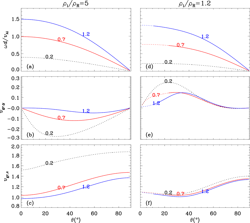
Figure 7: Dispersion properties of oblique quasi-kink modes in an asymmetric slab configuration, with the obliqueness measured by the angle $\theta$ between the equilibrium magnetic field $\bm{B}_{0}$ and a 2D wavevector $\bm{k}=k_{y}\bm{e}_{y}+k_{z}\bm{e}_{z}$. The combination $[\rho_{\rm i}/\rho_{\rm L},l/d]$ is fixed at $[10,0.3]$, whereas two values of $\rho_{\rm i}/\rho_{\rm R}$ are discriminated, one being $5$ (the left column) and the other being $1.2$ (right). Plotted are the $\theta$-dependencies of the oscillation frequency ($\omega$, the top row), the $y$-component of the group velocity ($v_{{\rm gr},y}$, middle), and (c) the $z$-component ($v_{{\rm gr},z}$, bottom). Several values of $kd$ are examined as labeled. The dotted (solid) portion in any curve corresponds to where $m_{\rm R}d<1/5$ ($m_{\rm R}d\geq 1/5$), with $m_{\rm R}d$ measuring the capability for the slab to trap oblique quasi-kink modes. See text for more details.

Figure 7 presents the $\theta$-dependencies of the oscillation frequency ($\omega$, the top row), the $y$-component of the group velocity ($v_{{\rm gr},y}$, middle), and the $z$-component ($v_{{\rm gr},z}$, bottom) for a number of values of $kd$ as labeled. Two values are examined for $\rho_{\rm i}/\rho_{\rm R}$, one being $5$ (the left column) and the other being $1.2$ (right). For any quantity, a solid curve is employed to connect its values for those $\theta$ where $m_{\rm R}d\geq 1/5$, whereas a dotted curve is adopted where the opposite is true. Note that a curve may not contain any solid or dotted portion, with the case for $kd=0.2$ ($kd=0.7$) in the left column being an example for the former (latter). Consider the left column first. One sees that the numerical results for both large and small values of $\theta$ are in excellent agreement with the analytical properties summarized for a “Fully Symmetric” configuration. This agreement occurs despite that the value adopted for $\rho_{\rm i}/\rho_{\rm R}$ in the resistive computations is quite some distance away from $\rho_{\rm i}/\rho_{\rm L}$. Particularly noteworthy is that $v_{{\rm gr},y}$ approaches zero from below when $\theta\to 90^{\circ}$ as anticipated (see Figure 7b). Likewise, $v_{{\rm gr},y}\to 0$ when $\theta\to 0$, and $v_{{\rm gr},y}$ for a given small $\theta$ is indeed negative (positive) when $kd$ is below (above) some threshold. This threshold $kd$ is nonetheless only marginally smaller than $1.2$, making the positive values of $v_{{\rm gr},y}$ at small $\theta$ for $kd=1.2$ differ little from zero. For the examined range of $kd$, it then holds in general that $v_{{\rm gr},y}$ tends to decrease with $\theta$ from zero to some local minimum before increasing towards zero when $\theta$ further increases. It also holds in general that $\omega$ monotonically decreases with $\theta$ for a fixed $k$, but is a monotonically increasing function of $k$ when $\theta$ is fixed (Figure 7a). Likewise, $v_{{\rm gr},z}$ turns out to increase (decrease) monotonically with $\theta$ ($k$) (Figure 7c). Now move on to the right column. The dispersion behavior is substantially more complicated, by which we mean particularly that some analytical expectations summarized for a “Fully Asymmetric” configuration do not apply. Take the behavior for $\theta\to 90^{\circ}$ for example. The numerically computed $v_{{\rm gr},y}$ is seen to approach zero from below rather than from above (Figure 7e), and $v_{{\rm gr},z}$ somehow decreases with $k$ rather than being $k$-independent (Figure 7f). These subtleties notwithstanding, our analytical expectations manage to capture some key features for us to proceed, the most noteworthy one being that $v_{{\rm gr},y}$ starts from being zero when $\theta\to 0$ and is consistently positive for small $\theta$. This feature, together with the analyitcal expectation that $v_{{\rm gr},y}$ is essentially zero for large $\theta$, then largely explain the behavior for $v_{{\rm gr},y}$ to be overall positive for the entire range of $\theta$. While only three values of $kd$ are presented, a parametric study indicates that the dispersion features, the sign of $v_{{\rm gr},y}$ in particular, are typical of what happens when $kd$ varies between $0.2$ and $1.2$. Consequently, that $m_{\rm R}d<1/5$ in some range of $\theta$ for some $kd$ does not seriously undermine the significance of Figure 7.

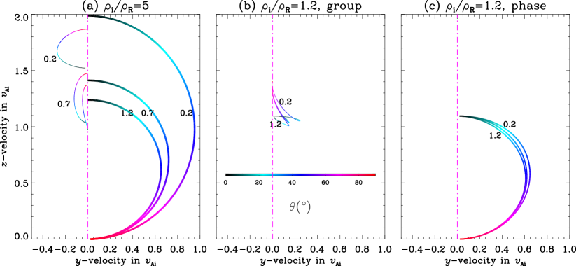
Figure 8: Phase (the thick curves) and group (thin) diagrams of oblique quasi-kink modes in an asymmetric slab configuration. The combination $[\rho_{\rm i}/\rho_{\rm L},l/d]$ is fixed at $[10,0.3]$, whereas two values of $\rho_{\rm i}/\rho_{\rm R}$ are discriminated, one being $5$ (the left panel) and the other being $1.2$ (the middle and right panels). The vertical dash-dotted line points in the direction of the equilibrium magnetic field $\bm{B}_{0}$. Any curve is color-coded by $\theta$, the angle that $\bm{k}$ makes with $\bm{B}_{0}$. See text for more details.

Figure 8 further collects the numerical results to produce the relevant phase and group diagrams, namely the trajectories that $\bm{v}_{\rm ph}$ (the thick curves) and $\bm{v}_{\rm gr}$ (thin) traverse in the velocity plane when $\theta$ varies. The magenta dash-dotted lines represent the vertical axis in this plane, pointing in the direction of the equilibrium magnetic field $\bm{B}_{0}$. Any curve is color-coded by $\theta$, and the pertinent value of $kd$ is placed adjacent to a curve when necessary. Note that the phase and group diagrams for $\rho_{\rm i}/\rho_{\rm R}=5$ are condensed into Figure 8a, whereas those for $\rho_{\rm i}/\rho_{\rm R}=1.2$ need to be plotted separately to avoid overlapping (Figures 8b and 8c). In comparison with Figure 7, one sees that Figure 8 better visualizes the differences in the dispersion behavior when different values are adopted for $\rho_{\rm i}/\rho_{\rm R}$. For instance, the $\bm{v}_{\rm ph}$ trajectories for $\rho_{\rm i}/\rho_{\rm R}=5$ are seen to possess a considerably stronger $k$-dependence than for $\rho_{\rm i}/\rho_{\rm R}=1.2$. Any $\bm{v}_{\rm gr}$ trajectory for $\rho_{\rm i}/\rho_{\rm R}=1.2$, on the other hand, tends to show a more complicated pattern, bending rather abruptly (e.g., $kd=1.2$) or even intersecting itself (e.g., $kd=0.7$) where the trajectory deviates the most from the $\bm{B}_{0}$-direction. More importantly, the $\bm{v}_{\rm gr}$ and $\bm{v}_{\rm ph}$ trajectories for $\rho_{\rm i}/\rho_{\rm R}=5$ are seen to lie essentially on opposite sides with respect to $\bm{B}_{0}$ (Figure 8a), whereas they are essentially located on the same side when $\rho_{\rm i}/\rho_{\rm R}=1.2$ (see Figures 8b and 8c). Evidently, this behavior derives from the difference in the signs of $v_{{\rm gr},y}$ between the computations with the two different values of $\rho_{\rm i}/\rho_{\rm R}$. Our discussions on $m_{\rm R}d$ therefore apply here as well, namely the significance of Figure 8 is not substantially compromised by the fact that $m_{\rm R}d$ may be small in some range of $\theta$ for some values of $kd$.

5.3 Discussion

We illustrate the observational implications of Figure 8 by considering the response of the asymmetric slab system therein to a small-amplitude exciter localized around the origin in all three directions. Recall that $\rho_{\rm i}/\rho_{\rm L}=10$. For the ease of description, let us suppose that the TLs are absent ($l=0$) even though our illustration is expected to hold unless the TLs are excessively thick. Suppose further that the initial perturbation is implemented via $v_{x}$. A close analogy can be drawn with the cylindrical study by Oliver et al. (2014, ORT14; also Oliver et al. 2015; Li et al. 2022). In general, both trapped modes (or equivalently “proper eigenmodes”) and improper continuum eigenmodes are excited. However, only trapped modes survive at large times, meaning that

$$v_{x}(x,y,z,t)=\int_{-\infty}^{\infty}dk_{y}\int_{-\infty}^{\infty}dk_{z}\sum_{j}\mathcal{F}_{j}(x;k_{y},k_{z}){\rm e}^{i(\omega_{j}t-k_{y}y-k_{z}z)}.$$ (38)

Briefly put, Equation (38) means that all values of $k_{y}$ and $k_{z}$ are involved given the localization of the initial perturbation. An EVP then ensues for any pair $[k_{y},k_{z}]$, the associated DR being Equation (34). The summation in Equation (38) incorporates all possible eigensolutions ($\omega_{j}$), with the contribution of the $j$-th solution (namely $\mathcal{F}_{j}$) determined by both its eigenfunction and the initial perturbation (see ORT14 for technical details). We proceed by assuming that only transverse fundamental quasi-kink modes are primarily excited, which is not that bold an assumption given the diversity of initial perturbations. The most straightforward application of Figure 8 then concerns the wave propagation in the $y$- and $z$-directions, meaning that it suffices to consider, say, the $x=0$ plane. Furthermore, we focus on those $(y,z,t)$ where the method of stationary phase (MSP) applies (e.g., Chapter 11 in W74). Seeing some $(y,z,t)$ as given, the MSP dictates that $v_{x}(x=0,y,z,t)$ is dominated by those wavepackets with central wavevectors $\bm{K}_{n}=K_{n,y}\bm{e}_{y}+K_{n,z}\bm{e}_{z}$ that solve

$$v_{{\rm gr},y}(\bm{K}_{n})=y/t,\quad v_{{\rm gr},z}(\bm{K}_{n})=z/t.$$ (39)

If $(y,z)$ is seen as variable, then the most prominent wave pattern at some given large time can be written as (see Equation (11.41) in W74)

$$v_{x}(x=0,y,z,t)\sim t^{-1}\sum_{n}\mathcal{G}_{n}(K_{n,y},K_{n,z}){\rm e}^{i\left[\omega(K_{n,y},K_{n,z})t-K_{n,y}y-K_{n,z}z\right]}.$$ (40)

Equation (40) can be seen as a predictive tool, the quantitative application of which is nonetheless not straightforward. One reason for us to say this is that Equation (40), while much simpler than Equation (38), still necessitates the summation over $n$ because the solution to Equation (39) is not unique even if only transverse fundamental quasi-kink modes arise. Regardless, the following morphological features can be predicted for those portions of a large-time wave pattern where most contributions come from the wavepackets with central wavevectors that lie in the range examined in Figure 8. For both values of $\rho_{\rm i}/\rho_{\rm R}$ therein, these portions will be concentrated around $\bm{B}_{0}$ (namely the $z$-axis) because so are the group trajectories. We deem this feature somehow striking because the fluid in the $x=0$ plane itself is uniform and the waves nonetheless belong to the fast family. Some subtle differences are then expected in the wave patterns for different values of $\rho_{\rm i}/\rho_{\rm R}$, to illustrate which point it suffices to consider positive $y$ and $z$. When $\rho_{\rm i}/\rho_{\rm R}=5$, the difference in the signs between $v_{{\rm gr},y}$ and $v_{{\rm ph},y}$ means that some iso-phase curves (say, where $v_{x}(x=0,y,z,t)=0$) will propagate toward the $z$-axis as time proceeds. In contrast, that $v_{{\rm gr},y}$ and $v_{{\rm ph},y}$ essentially possess the same sign for $\rho_{\rm i}/\rho_{\rm R}=1.2$ dictates that the associated iso-phase curves propagate away from the $z$-axis. Evidently, all these qualitative predictions need to be tested against time-dependent 3D numerical simulations, which have yet to conducted even for “Fully Symmetric” or “Fully Asymmetric” slabs to our knowledge despite the abundance of 2D ones (e.g., Murawski & Roberts, 1993; Ogrodowczyk & Murawski, 2006; Pascoe et al., 2013; Kolotkov et al., 2021; Guo et al., 2022). However, it is safe to conclude that our study highlights the importance of the phase and group trajectories as at least the first step toward a thorough understanding of the necessarily complicated 3D wave patterns in structured media. Conversely, these 3D patterns can be employed for seismological purposes, which looks promising given that stereoscopic techniques tend to mature with time (see e.g., Aschwanden, 2011, for a review) and have been employed in initial examinations on impulsively excited waves in, say, streamer stalks (Decraemer et al., 2020).

6 Summary

This study was largely motivated by some intensive recent interest in small-amplitude magnetoacoustic waves in static, straight, field-aligned, one-dimensional equilibria where the exteriors of a magnetic slab are different between the two sides (e.g., Allcock & Erdélyi, 2017; Zsámberger et al., 2018; Zsámberger & Erdélyi, 2021). We chose to work with zero-beta MHD such that the inhomogeneity is entirely in the equilibrium density $\rho_{0}(x)$, from which a uniform slab (with density $\rho_{\rm i}$) and its two uniform exteriors (with densities $\rho_{\rm L}$ and $\rho_{\rm R}$) are identified. By “left” we refer to the side that ensures $\rho_{\rm L}\leq\rho_{\rm R}$. Two aspects make our study new, one being that $\rho_{0}(x)$ is not piece-wise constant but varies continuously over some transition layer (TL) between the slab and either exterior, the other being that out-of-plane propagation is addressed ($k_{y}\neq 0$). Oblique quasi-kink modes, the focus of this study, are therefore absorbed via the Alfv$\acute{\rm e}$n resonance, their dispersion properties consistently computed with a resistive eigenmode approach. We additionally made some analytical progress in the thin-boundary (TB) limit, deriving a dispersion relation (DR, Equation (22)) for generic asymmetric configurations, and extending previous analytical studies on “Fully Symmetric” ($\rho_{\rm R}=\rho_{\rm L}$) or “Fully Asymmetric” ($\rho_{\rm R}=\rho_{\rm i}$) setups. Our findings can be summarized as follows.

Two features stand out in our results on resonant absorption. Technically, our resistive computations demonstrated that the TB expectations may hold well beyond their nominal range of applicability, thereby corroborating similar conclusions drawn for different coronal configurations. Physically, we found that the absorption rates may possess a nonmonotonic $\rho_{\rm i}/\rho_{\rm R}$-dependence when $\rho_{\rm i}/\rho_{\rm R}$ varies from the “Fully Symmetric” to the “Fully Asymmetric” limit. An energetics analysis yields that this behavior results from the difference between the two Alfv$\acute{\rm e}$n continua, which means particularly that the right resonance comes into play only when $\rho_{\rm i}/\rho_{\rm R}$ exceeds some threshold $(\rho_{\rm i}/\rho_{\rm R})_{\rm crit}$. Given the likely onset of the Kelvin-Helmholtz instability, we argued that two qualitatively different regimes may arise in the morphology of a coronal arcade when oscillating in a vertically polarized kink mode. While only one edge may be deformed when $\rho_{\rm i}/\rho_{\rm R}<(\rho_{\rm i}/\rho_{\rm R})_{\rm crit}$, both edges may be subject to deformation or even corrugation when the opposite is true.

We also examined oblique quasi-kink modes from the perspective of phase and group diagrams, an aspect that has not been addressed to our knowledge. We restricted ourselves to only two considerably different values of $\rho_{\rm i}/\rho_{\rm R}$. The group diagrams, namely the trajectories that the group velocity traverses in the velocity plane, share the similarity that they are concentrated around the equilibrium magnetic field $\bm{B}_{0}=B_{0}\bm{e}_{z}$. However, one key difference between the two sets of computations is that the phase and group trajectories lie essentially on the same side (different sides) relative to $\bm{B}_{0}$ when the equilibrium setup is not far from a “Fully Asymmetric” (“Fully Symmetric”) one. We placed our findings in the context of impulsively excited quasi-kink waves in slab-like configurations, expecting the following large-time behavior in the $y-z$ cut through the slab axis. Common to both $\rho_{\rm i}/\rho_{\rm R}$, the wave patterns are likely to be highly anisotropic, extending only to a limited angular distance from $\bm{B}_{0}$. However, some iso-phase curves may propagate toward (away from) $\bm{B}_{0}$ as time proceeds when the equilibrium is close to a “Fully Symmetric” (“Fully Asymmetric”) configuration.

Figure 3: Dispersion properties of resonantly damped oblique quasi-kink modes in an asymmetric slab configuration. Plotted here are the oscillation frequency ($\omega$, the upper row) and the ratio of the damping rate to the oscillation frequency ($-\gamma/\omega$, lower) against the dimensionless TL width ($l/d$). A fixed combination $[\rho_{\rm i}/\rho_{\rm L},k_{y}d,k_{z}d]=[10,0.5,\pi/50]$ is adopted, whereas a number of $\rho_{\rm i}/\rho_{\rm R}$ are examined as discriminated by the line styles. The black curves represent our resistive computations (labeled “Resis”). Also presented are two groups of solutions to the dispersion relation (Equation (22)) in the thin-boundary limit, one found numerically (labeled “TB num”, the red curves in the left column) and the other found analytically in an approximate manner (“TB analytic”, the blue curves in the right column). See text for more details.

References

- Allcock & Erdélyi (2017) Allcock, M., & Erdélyi, R. 2017, Sol. Phys., 292, 35, doi: 10.1007/s11207-017-1054-y
- Allcock & Erdélyi (2018) —. 2018, ApJ, 855, 90, doi: 10.3847/1538-4357/aaad0c
- Allcock et al. (2019) Allcock, M., Shukhobodskaia, D., Zsámberger, N. K., & Erdélyi, R. 2019, Frontiers in Astronomy and Space Sciences, 6, 48, doi: 10.3389/fspas.2019.00048
- Allian et al. (2019) Allian, F., Jain, R., & Hindman, B. W. 2019, ApJ, 880, 3, doi: 10.3847/1538-4357/ab264c
- Andries & Goossens (2007) Andries, J., & Goossens, M. 2007, Physics of Plasmas, 14, 052101, doi: 10.1063/1.2714513
- Andries et al. (2000) Andries, J., Tirry, W. J., & Goossens, M. 2000, ApJ, 531, 561, doi: 10.1086/308430
- Antolin & Van Doorsselaere (2019) Antolin, P., & Van Doorsselaere, T. 2019, Frontiers in Physics, 7, 85, doi: 10.3389/fphy.2019.00085
- Antolin et al. (2014) Antolin, P., Yokoyama, T., & Van Doorsselaere, T. 2014, ApJ, 787, L22, doi: 10.1088/2041-8205/787/2/L22
- Arregui (2015) Arregui, I. 2015, Philosophical Transactions of the Royal Society of London Series A, 373, 20140261, doi: 10.1098/rsta.2014.0261
- Arregui et al. (2007) Arregui, I., Terradas, J., Oliver, R., & Ballester, J. L. 2007, Sol. Phys., 246, 213, doi: 10.1007/s11207-007-9041-3
- Aschwanden (2011) Aschwanden, M. J. 2011, Living Reviews in Solar Physics, 8, 5, doi: 10.12942/lrsp-2011-5
- Aschwanden et al. (2004) Aschwanden, M. J., Nakariakov, V. M., & Melnikov, V. F. 2004, ApJ, 600, 458, doi: 10.1086/379789
- Banerjee et al. (2021) Banerjee, D., Krishna Prasad, S., Pant, V., et al. 2021, Space Sci. Rev., 217, 76, doi: 10.1007/s11214-021-00849-0
- Barbulescu & Erdélyi (2018) Barbulescu, M., & Erdélyi, R. 2018, Sol. Phys., 293, 86, doi: 10.1007/s11207-018-1305-6
- Brady & Arber (2005) Brady, C. S., & Arber, T. D. 2005, A&A, 438, 733, doi: 10.1051/0004-6361:20042527
- Braginskii (1965) Braginskii, S. I. 1965, Reviews of Plasma Physics, 1, 205
- Browning & Priest (1984) Browning, P. K., & Priest, E. R. 1984, A&A, 131, 283
- Cally (1991) Cally, P. S. 1991, Journal of Plasma Physics, 45, 453, doi: 10.1017/S002237780001583X
- Chen & Hasegawa (1974) Chen, L., & Hasegawa, A. 1974, Physics of Fluids, 17, 1399, doi: 10.1063/1.1694904
- Chen et al. (2018) Chen, S.-X., Li, B., Shi, M., & Yu, H. 2018, ApJ, 868, 5, doi: 10.3847/1538-4357/aae686
- Chen et al. (2021) Chen, S.-X., Li, B., Van Doorsselaere, T., et al. 2021, ApJ, 908, 230, doi: 10.3847/1538-4357/abd7f3
- Chen et al. (2011) Chen, Y., Feng, S. W., Li, B., et al. 2011, ApJ, 728, 147, doi: 10.1088/0004-637X/728/2/147
- Chen et al. (2010) Chen, Y., Song, H. Q., Li, B., et al. 2010, ApJ, 714, 644, doi: 10.1088/0004-637X/714/1/644
- De Moortel & Browning (2015) De Moortel, I., & Browning, P. 2015, Philosophical Transactions of the Royal Society of London Series A, 373, 20140269, doi: 10.1098/rsta.2014.0269
- De Moortel & Nakariakov (2012) De Moortel, I., & Nakariakov, V. M. 2012, Philosophical Transactions of the Royal Society of London Series A, 370, 3193, doi: 10.1098/rsta.2011.0640
- Decraemer et al. (2020) Decraemer, B., Zhukov, A. N., & Van Doorsselaere, T. 2020, ApJ, 893, 78, doi: 10.3847/1538-4357/ab8194
- Díaz et al. (2006) Díaz, A. J., Zaqarashvili, T., & Roberts, B. 2006, A&A, 455, 709, doi: 10.1051/0004-6361:20054430
- Edwin & Roberts (1982) Edwin, P. M., & Roberts, B. 1982, Sol. Phys., 76, 239, doi: 10.1007/BF00170986
- Edwin & Roberts (1983) —. 1983, Sol. Phys., 88, 179, doi: 10.1007/BF00196186
- Erdélyi & Morton (2009) Erdélyi, R., & Morton, R. J. 2009, A&A, 494, 295, doi: 10.1051/0004-6361:200810318
- Giagkiozis et al. (2016) Giagkiozis, I., Goossens, M., Verth, G., Fedun, V., & Van Doorsselaere, T. 2016, ApJ, 823, 71, doi: 10.3847/0004-637X/823/2/71
- Gijsen & Van Doorsselaere (2014) Gijsen, S. E., & Van Doorsselaere, T. 2014, A&A, 562, A38, doi: 10.1051/0004-6361/201322755
- Goedbloed et al. (2019) Goedbloed, H., Keppens, R., & Poedts, S. 2019, Magnetohydrodynamics of Laboratory and Astrophysical Plasmas (Cambridge University Press), doi: 10.1017/9781316403679
- Goossens et al. (2006) Goossens, M., Andries, J., & Arregui, I. 2006, Philosophical Transactions of the Royal Society of London Series A, 364, 433, doi: 10.1098/rsta.2005.1708
- Goossens et al. (2012) Goossens, M., Andries, J., Soler, R., et al. 2012, ApJ, 753, 111, doi: 10.1088/0004-637X/753/2/111
- Goossens et al. (2021) Goossens, M., Chen, S. X., Geeraerts, M., Li, B., & Van Doorsselaere, T. 2021, A&A, 646, A86, doi: 10.1051/0004-6361/202039780
- Goossens et al. (2011) Goossens, M., Erdélyi, R., & Ruderman, M. S. 2011, Space Sci. Rev., 158, 289, doi: 10.1007/s11214-010-9702-7
- Goossens et al. (1992) Goossens, M., Hollweg, J. V., & Sakurai, T. 1992, Sol. Phys., 138, 233, doi: 10.1007/BF00151914
- Goossens et al. (2014) Goossens, M., Soler, R., Terradas, J., Van Doorsselaere, T., & Verth, G. 2014, ApJ, 788, 9, doi: 10.1088/0004-637X/788/1/9
- Goossens et al. (2009) Goossens, M., Terradas, J., Andries, J., Arregui, I., & Ballester, J. L. 2009, A&A, 503, 213, doi: 10.1051/0004-6361/200912399
- Goossens et al. (2013) Goossens, M., Van Doorsselaere, T., Soler, R., & Verth, G. 2013, ApJ, 768, 191, doi: 10.1088/0004-637X/768/2/191
- Grossmann & Tataronis (1973) Grossmann, W., & Tataronis, J. 1973, Zeitschrift fur Physik, 261, 217, doi: 10.1007/BF01391914
- Guo et al. (2020) Guo, M., Li, B., & Van Doorsselaere, T. 2020, ApJ, 904, 116, doi: 10.3847/1538-4357/abc1df
- Guo et al. (2022) Guo, M., Li, B., Van Doorsselaere, T., & Shi, M. 2022, MNRAS, 515, 4055, doi: 10.1093/mnras/stac2006
- Guo et al. (2016) Guo, M.-Z., Chen, S.-X., Li, B., Xia, L.-D., & Yu, H. 2016, Sol. Phys., 291, 877, doi: 10.1007/s11207-016-0868-3
- Hasegawa & Chen (1974) Hasegawa, A., & Chen, L. 1974, Phys. Rev. Lett., 32, 454, doi: 10.1103/PhysRevLett.32.454
- Heyvaerts & Priest (1983) Heyvaerts, J., & Priest, E. R. 1983, A&A, 117, 220
- Hindman & Jain (2015) Hindman, B. W., & Jain, R. 2015, ApJ, 814, 105, doi: 10.1088/0004-637X/814/2/105
- Hindman & Jain (2018) —. 2018, ApJ, 858, 6, doi: 10.3847/1538-4357/aab9b1
- Hollweg & Yang (1988) Hollweg, J. V., & Yang, G. 1988, J. Geophys. Res., 93, 5423, doi: 10.1029/JA093iA06p05423
- Ionson (1978) Ionson, J. A. 1978, ApJ, 226, 650, doi: 10.1086/156648
- Jain et al. (2015) Jain, R., Maurya, R. A., & Hindman, B. W. 2015, ApJ, 804, L19, doi: 10.1088/2041-8205/804/1/L19
- Jess et al. (2015) Jess, D. B., Morton, R. J., Verth, G., et al. 2015, Space Sci. Rev., 190, 103, doi: 10.1007/s11214-015-0141-3
- Khomenko & Collados (2015) Khomenko, E., & Collados, M. 2015, Living Reviews in Solar Physics, 12, 6, doi: 10.1007/lrsp-2015-6
- Kolotkov et al. (2021) Kolotkov, D. Y., Nakariakov, V. M., Moss, G., & Shellard, P. 2021, MNRAS, 505, 3505, doi: 10.1093/mnras/stab1587
- Kwon et al. (2013) Kwon, R.-Y., Ofman, L., Olmedo, O., et al. 2013, ApJ, 766, 55, doi: 10.1088/0004-637X/766/1/55
- Lee & Roberts (1986) Lee, M. A., & Roberts, B. 1986, ApJ, 301, 430, doi: 10.1086/163911
- Leroy (1985) Leroy, B. 1985, Geophysical and Astrophysical Fluid Dynamics, 32, 123, doi: 10.1080/03091928508208781
- Li et al. (2020) Li, B., Antolin, P., Guo, M. Z., et al. 2020, Space Sci. Rev., 216, 136, doi: 10.1007/s11214-020-00761-z
- Li et al. (2022) Li, B., Chen, S.-X., & Li, A.-L. 2022, ApJ, 928, 33, doi: 10.3847/1538-4357/ac5402
- Lopin (2022) Lopin, I. 2022, MNRAS, 514, 4329, doi: 10.1093/mnras/stac1502
- Lopin & Nagorny (2015) Lopin, I., & Nagorny, I. 2015, ApJ, 810, 87, doi: 10.1088/0004-637X/810/2/87
- Luna et al. (2008) Luna, M., Terradas, J., Oliver, R., & Ballester, J. L. 2008, ApJ, 676, 717, doi: 10.1086/528367
- Luna et al. (2009) —. 2009, ApJ, 692, 1582, doi: 10.1088/0004-637X/692/2/1582
- Morton & Ruderman (2011) Morton, R. J., & Ruderman, M. S. 2011, A&A, 527, A53, doi: 10.1051/0004-6361/201016028
- Murawski & Roberts (1993) Murawski, K., & Roberts, B. 1993, Sol. Phys., 144, 101, doi: 10.1007/BF00667986
- Nakariakov & Kolotkov (2020) Nakariakov, V. M., & Kolotkov, D. Y. 2020, ARA&A, 58, 441, doi: 10.1146/annurev-astro-032320-042940
- Nakariakov & Verwichte (2005) Nakariakov, V. M., & Verwichte, E. 2005, Living Reviews in Solar Physics, 2, 3, doi: 10.12942/lrsp-2005-3
- Ogrodowczyk & Murawski (2006) Ogrodowczyk, R., & Murawski, K. 2006, Sol. Phys., 236, 273, doi: 10.1007/s11207-006-0018-4
- Oliver et al. (2014) Oliver, R., Ruderman, M. S., & Terradas, J. 2014, ApJ, 789, 48, doi: 10.1088/0004-637X/789/1/48
- Oliver et al. (2015) —. 2015, ApJ, 806, 56, doi: 10.1088/0004-637X/806/1/56
- Oxley et al. (2020a) Oxley, W., Zsámberger, N. K., & Erdélyi, R. 2020a, ApJ, 890, 109, doi: 10.3847/1538-4357/ab67b3
- Oxley et al. (2020b) —. 2020b, ApJ, 898, 19, doi: 10.3847/1538-4357/ab9639
- Pascoe & Nakariakov (2016) Pascoe, D. J., & Nakariakov, V. M. 2016, A&A, 593, A52, doi: 10.1051/0004-6361/201526546
- Pascoe et al. (2013) Pascoe, D. J., Nakariakov, V. M., & Kupriyanova, E. G. 2013, A&A, 560, A97, doi: 10.1051/0004-6361/201322678
- Poedts & Kerner (1991) Poedts, S., & Kerner, W. 1991, Phys. Rev. Lett., 66, 2871, doi: 10.1103/PhysRevLett.66.2871
- Rial et al. (2010) Rial, S., Arregui, I., Terradas, J., Oliver, R., & Ballester, J. L. 2010, ApJ, 713, 651, doi: 10.1088/0004-637X/713/1/651
- Rial et al. (2013) —. 2013, ApJ, 763, 16, doi: 10.1088/0004-637X/763/1/16
- Roberts (1981a) Roberts, B. 1981a, Sol. Phys., 69, 27, doi: 10.1007/BF00151253
- Roberts (1981b) —. 1981b, Sol. Phys., 69, 39, doi: 10.1007/BF00151254
- Roberts (2019) Roberts, B. 2019, MHD Waves in the Solar Atmosphere (Cambridge University Press), doi: 10.1017/9781108613774
- Robertson & Ruderman (2011) Robertson, D., & Ruderman, M. S. 2011, A&A, 525, A4, doi: 10.1051/0004-6361/201015525
- Robertson et al. (2010) Robertson, D., Ruderman, M. S., & Taroyan, Y. 2010, A&A, 515, A33, doi: 10.1051/0004-6361/201014055
- Rosenberg (1970) Rosenberg, H. 1970, A&A, 9, 159
- Ruderman (2003) Ruderman, M. S. 2003, A&A, 409, 287, doi: 10.1051/0004-6361:20031079
- Ruderman & Roberts (2002) Ruderman, M. S., & Roberts, B. 2002, ApJ, 577, 475, doi: 10.1086/342130
- Ruderman et al. (1995) Ruderman, M. S., Tirry, W., & Goossens, M. 1995, Journal of Plasma Physics, 54, 129, doi: 10.1017/S0022377800018407
- Sakurai et al. (1991) Sakurai, T., Goossens, M., & Hollweg, J. V. 1991, Sol. Phys., 133, 227, doi: 10.1007/BF00149888
- Schrijver (2007) Schrijver, C. J. 2007, ApJ, 662, L119, doi: 10.1086/519455
- Schrijver et al. (2002) Schrijver, C. J., Aschwanden, M. J., & Title, A. M. 2002, Sol. Phys., 206, 69, doi: 10.1023/A:1014957715396
- Sewell (1988) Sewell, G. 1988, The Numerical Solution of Ordinary and Partial Differential Equations (San Diego: Academic Press)
- Shukhobodskaia & Erdélyi (2018) Shukhobodskaia, D., & Erdélyi, R. 2018, ApJ, 868, 128, doi: 10.3847/1538-4357/aae83c
- Soler et al. (2013) Soler, R., Goossens, M., Terradas, J., & Oliver, R. 2013, ApJ, 777, 158, doi: 10.1088/0004-637X/777/2/158
- Soler & Luna (2015) Soler, R., & Luna, M. 2015, A&A, 582, A120, doi: 10.1051/0004-6361/201526919
- Soler & Terradas (2015) Soler, R., & Terradas, J. 2015, ApJ, 803, 43, doi: 10.1088/0004-637X/803/1/43
- Tataronis & Grossmann (1973) Tataronis, J., & Grossmann, W. 1973, Zeitschrift fur Physik, 261, 203, doi: 10.1007/BF01391913
- Tatsuno & Wakatani (1998) Tatsuno, T., & Wakatani, M. 1998, Journal of the Physical Society of Japan, 67, 2322, doi: 10.1143/JPSJ.67.2322
- Terradas et al. (2008) Terradas, J., Andries, J., Goossens, M., et al. 2008, ApJ, 687, L115, doi: 10.1086/593203
- Terradas et al. (2006) Terradas, J., Oliver, R., & Ballester, J. L. 2006, ApJ, 642, 533, doi: 10.1086/500730
- Thackray & Jain (2017) Thackray, H., & Jain, R. 2017, A&A, 608, A108, doi: 10.1051/0004-6361/201731193
- Tirry & Goossens (1996) Tirry, W. J., & Goossens, M. 1996, ApJ, 471, 501, doi: 10.1086/177986
- Van Doorsselaere et al. (2004) Van Doorsselaere, T., Andries, J., Poedts, S., & Goossens, M. 2004, ApJ, 606, 1223, doi: 10.1086/383191
- Van Doorsselaere et al. (2014) Van Doorsselaere, T., Gijsen, S. E., Andries, J., & Verth, G. 2014, ApJ, 795, 18, doi: 10.1088/0004-637X/795/1/18
- Van Doorsselaere et al. (2008) Van Doorsselaere, T., Ruderman, M. S., & Robertson, D. 2008, A&A, 485, 849, doi: 10.1051/0004-6361:200809841
- Van Doorsselaere et al. (2020) Van Doorsselaere, T., Srivastava, A. K., Antolin, P., et al. 2020, Space Sci. Rev., 216, 140, doi: 10.1007/s11214-020-00770-y
- Vasheghani Farahani et al. (2014) Vasheghani Farahani, S., Hornsey, C., Van Doorsselaere, T., & Goossens, M. 2014, ApJ, 781, 92, doi: 10.1088/0004-637X/781/2/92
- Verwichte et al. (2006a) Verwichte, E., Foullon, C., & Nakariakov, V. M. 2006a, A&A, 446, 1139, doi: 10.1051/0004-6361:20053955
- Verwichte et al. (2006b) —. 2006b, A&A, 449, 769, doi: 10.1051/0004-6361:20054398
- Verwichte et al. (2005) Verwichte, E., Nakariakov, V. M., & Cooper, F. C. 2005, A&A, 430, L65, doi: 10.1051/0004-6361:200400133
- Verwichte et al. (2004) Verwichte, E., Nakariakov, V. M., Ofman, L., & Deluca, E. E. 2004, Sol. Phys., 223, 77, doi: 10.1007/s11207-004-0807-6
- Wang et al. (2021) Wang, T., Ofman, L., Yuan, D., et al. 2021, Space Sci. Rev., 217, 34, doi: 10.1007/s11214-021-00811-0
- Wang & Solanki (2004) Wang, T. J., & Solanki, S. K. 2004, A&A, 421, L33, doi: 10.1051/0004-6361:20040186
- Wang et al. (2008) Wang, T. J., Solanki, S. K., & Selwa, M. 2008, A&A, 489, 1307, doi: 10.1051/0004-6361:200810230
- Wentzel (1979a) Wentzel, D. G. 1979a, A&A, 76, 20
- Wentzel (1979b) —. 1979b, ApJ, 227, 319, doi: 10.1086/156732
- Wentzel (1979c) —. 1979c, ApJ, 233, 756, doi: 10.1086/157437
- Whitham (1974) Whitham, G. 1974, Linear and Nonlinear Waves (Wiley). https://books.google.nl/books?id=f8oRAQAAIAAJ
- Wilhelm et al. (2011) Wilhelm, K., Abbo, L., Auchère, F., et al. 2011, A&A Rev., 19, 35, doi: 10.1007/s00159-011-0035-7
- Yu et al. (2021) Yu, H., Li, B., Chen, S., & Guo, M. 2021, Sol. Phys., 296, 95, doi: 10.1007/s11207-021-01839-9
- Yu et al. (2017) Yu, H., Li, B., Chen, S.-X., Xiong, M., & Guo, M.-Z. 2017, ApJ, 836, 1, doi: 10.3847/1538-4357/836/1/1
- Zajtsev & Stepanov (1975) Zajtsev, V. V., & Stepanov, A. V. 1975, Issledovaniia Geomagnetizmu Aeronomii i Fizike Solntsa, 37, 3
- Zsámberger et al. (2018) Zsámberger, N. K., Allcock, M., & Erdélyi, R. 2018, ApJ, 853, 136, doi: 10.3847/1538-4357/aa9ffe
- Zsámberger & Erdélyi (2020) Zsámberger, N. K., & Erdélyi, R. 2020, ApJ, 894, 123, doi: 10.3847/1538-4357/ab8791
- Zsámberger & Erdélyi (2021) —. 2021, ApJ, 906, 122, doi: 10.3847/1538-4357/abca9d
- Zsámberger & Erdélyi (2022) —. 2022, ApJ, 934, 155, doi: 10.3847/1538-4357/ac7be3
- Zsámberger et al. (2022a) Zsámberger, N. K., Sánchez Montoya, C. M., & Erdélyi, R. 2022a, ApJ, 937, 23, doi: 10.3847/1538-4357/ac8427
- Zsámberger et al. (2022b) Zsámberger, N. K., Tong, Y., Asztalos, B., & Erdélyi, R. 2022b, ApJ, 935, 41, doi: 10.3847/1538-4357/ac7ebf