A Survey on Causal Representation Learning and Future Work for Medical Image Analysis

Abstract

Statistical machine learning algorithms have achieved state-of-the-art results on benchmark datasets, outperforming humans in many tasks. However, the out-of-distribution data and confounder, which have an unpredictable causal relationship, significantly degrade the performance of the existing models. Causal Representation Learning (CRL) has recently been a promising direction to address the causal relationship problem in vision understanding. This survey presents recent advances in CRL in vision. Firstly, we introduce the basic concept of causal inference. Secondly, we analyze the CRL theoretical work, especially in invariant risk minimization, and the practical work in feature understanding and transfer learning. Finally, we propose a future research direction in medical image analysis and CRL general theory.

1 Introduction

Correlation does not imply causation geer2011correlation . One famous example is the Simpson’s paradoxwagner1982simpson (see Fig. 1). Even if the series of events do have causality, it is hard to distinguish that relationship. One effective way of learning causality is to conduct a randomized controlled trial (RCT), randomly assigning participants into a treatment group or a control group so that people can observe the effect via the outcome variable. However, RCT is inflexible because it targets the sample average, which makes the mechanism unclear. Another widely used information type is observational data, which records every event that could be observed. Nowadays, machine learning algorithms attempt to learn patterns by fitting the observational data, losing sight of the causality. This results in poor performance when generalizing the model to an unseen distribution or learning the wrong causality.

To escape the dilemma mentioned above, Pearl firstly introduced a causality system with the three-layer causal hierarchy, called Pearl Causal Hierarchy (PCH), which contains Association, Intervention, and Counterfactualspearl2009causal pearl2 pearl2009causality . To support this theory, Pearl developed structural causal model (SCM), which combines structural equation models (SEM), potential outcome framework, and the directed acyclic graphs (DAG)description1 description2 description3 description4 description5 for probabilistic reasoning and causal analysis, typically using the do-calculusdo1 . With these tools, causal analysis infers probabilities under not only statistical conditions but also the dynamics of probabilities under changing conditions pearl2009causality . Currently, causal inference is a popular research direction with comprehensive literature yao2021survey imbens2015causal gangl2010causal bareinboim2022pearl zhang2021causal , and is widely applied in decision evaluation (e.g. healthcare), counterfactual estimation (e.g. representation learning methods), and dealing with selection bias (e.g. advertising, recommendation) yao2021survey .

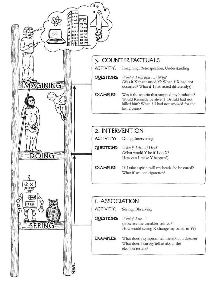
Figure 1: Three levels of Pearl Causal Hierarchy (PCH). (Drawing by picture ) The first level is association $P(y|x)$,(e.g. supervised or unsupervised learning). The second level is intervention $P(y|do(x),c)$, e.g.(feature learning, few-show learning). The third level is counterfactual $P(y_{x}|x^{\prime},y^{\prime})$, (e.g. zero-shot learning, long-tailed classification.)

Although most of the causal inference could be applied in low-dimensional data (e.g., tabular data, describable events), research in high-dimensional data is still a struggle. In computer vision, for example, which often suffers from confounder that the model tends to classify a cow in dessert as a camel. The invention of advanced network architecture (i.e. resnethe2016deep ,transformervaswani2017attention , etc.) may even enhance this misunderstanding. Recently, much research introduced the task-driven solution, attempting to discover the fundamental mechanism. (e.g. in image deraining, ren2019progressive zheng2022sapnet jiang2020multi introduced the progressive algorithm, in low-light image enhancement, cuiyou imitate the principle of camera imaging, in point cloud analysis, qi2017pointnet qi2017pointnet++ introduced point abstraction.) However, these models still struggle in o.o.d prediction.

Causal representation learning (CRL) is a useful tool to unscramble mechanisms. CRL assumes the data are latent causal variables that are causal related and satisfy conditional SCM, using non-linear mapping. With this assumption, CRL could discover the causal relationship via estimating the distribution after intervention if the causal latent variable and SCM are learnable. Moreover, CRL could even imagine the unseen data according to the counterfactual results, making models robust in the o.o.d prediction. However, distinguishing the confounder and discovering the SCM is very challenging. Therefore, some assumptions like sparsity and independent causal mechanism are introduced as an inductive bias in CRLscholkopf2021toward . Recently, theoretical works with CRL have been developed (e.g. Low-ranklow1 low2 , Generalized Independent Noise conditiongin1 gin2 , invariant risk minimizationd1-irm1 ; d1-irm2 ; d1-irm3 ; d1-irm4 ; d1-irm5 ; d1-irm6 ; d1-irm7 ; d1-irm8 ) and has shown promising performance in feature understanding (e.g. scene graph generation, pretraining, long-tailed data)wang2020visual tang2020unbiased f5 ; f6 ; f7 ; f8 ; f9 ; f10 ; f11 ; f12 ; f13 ; f14 ; f15 and transfer learning problem (e.g. adversarial methods, generalization, adaptation)d2-domain1 ; d2-domain2 ; d2-domain3 ; subbaswamy2020spec ; d2-domain4 ; d2-domain5 .

In this paper, we present a survey on CRL about its recent advances, with a special focus on the basic concept of causal inference (section 2), theoretical work, practical work(section 3), and future research directions in medical image analysismed3 (section 4).

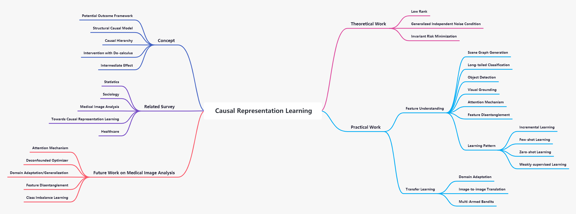
Figure 2: The mindmap of causal representation learning in vision

2 Concept of Causal Inference

	Condition
Treatment	Mild	Severe	Total	Causal
A	15% (210/1400)	30% (30/100)	16% (240/1500)	19.4%
B	10% (5/50)	20% (100/500)	19% (105/550)	12.9%

Table 1: The example of Simpson’s paradox. Although the total deaths of treatment A is less than deaths of treatment B, the treatment B is a worthy choice in terms of causal analysis. In naive method, for example, the treatment effect of A (16%), is given by $\frac{1400}{1500}(0.15)+\frac{100}{1500}(0.30)$. In causal analysis, the treatment effect of A (19.4%) is given by $\frac{1450}{2050}(0.15)+\frac{600}{2050}(0.30)$.

In this section, several concepts of causal reasoning are introduced, including potential outcome framework, structural causal model(SCM), and causal graphs via do-calculus.

2.1 Potential outcome framework

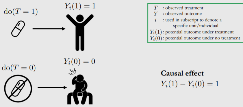
Figure 3: Example of the potential outcomes (Drawn by neal2020introduction ). The treatment effect are measured on whether to take the drug or not.

An example in Fig.3 shows how the potential outcomes framework works. However, we are in a dilemma that we cannot observe the causal effect on the same person. If one person takes the drug, we will lose the information of the person not taking the drug. This dilemma is known as the ”fundamental problem of causal inference”zhang2021causal .

2.2 Structural Causal Model

Firstly, we define the symbols.

• $X$, random variable

• $P\left(Y_{x}\right):=P(Y\mid do(X=x))$

• path $(X,Y)$: any path from X to Y.

• collider $Z$, $X\rightarrow Z\leftarrow Y,X\perp Y,X\not\perp Y\mid Z$.

The structural causal modelpearl2009causal pearl2009causality is a 4-tuple $\langle\mathbf{U},\mathbf{V},\mathcal{F},P(\mathbf{U})\rangle$, where:

• $\mathbf{U}$ is a set of background variables (exogenous variables), determined by factors outside the model.

• $\mathbf{V}$ is a set $\left\{V_{1},V_{2},\ldots,V_{n}\right\}$ of variables, called endogenous, determined by other variables within the model

• $\mathcal{F}$ is a set of functions $\left\{f_{1},f_{2},\ldots,f_{n}\right\}$, each $f_{i}$ is a mapping from $U_{i}\cup PA_{i}$(PA: parents) to $V_{i}$, where $U_{i}\subseteq U$ and $PA_{i}$ is a set of causes of $V_{i}$. The entire set $\mathcal{F}$ forms a mapping from $\mathbf{U}$ to $\mathbf{V}$. That is, for $i$ = 1,…,n, $v_{i}\leftarrow f_{i}\left(pa_{i},v_{i}\right)$.

• $P(\mathbf{U})$ is a probability function defined over the domain of $\mathbf{U}$.

For example, suppose that there exists a causal relationship between treatment solution $X$ and lung function $Y$ of an asthma patient. Simultaneously, suppose that $Y$ also relies on the level of air pollution $Z$. Under this circumstance, $X$ and $Y$ are endogenous variables, $Z$ is exogenous variables. Therefore, the SCM can be instantiated as,

$$U=\{Z,U_{x},U_{y}\},V=\{X,Y\},F=\{f_{X},f_{Y}\}$$ (1)

$$f_{X}:X\leftarrow f_{X}(U_{x})$$

$$f_{Y}:Y\leftarrow f_{Y}(X,Z,U_{y})$$

2.3 Causal Hierarchy

2.3.1 Level1 seeing

For any SCM, the formula,

$$P^{\mathcal{M}}(\mathbf{Y}=\mathbf{y})=\sum_{\{\mathbf{u}\mid\mathbf{Y}(\mathbf{u})=\mathbf{y}\}}P(\mathbf{u})$$ (2)

could estimate any joint distribution of $\mathbf{Y}\subset\mathbf{V}$ given by $\mathbf{Y}(U=u)$. Take the image classification task as an example. $\mathbf{V}=\mathbf{X}\bigcup\mathbf{Y}$, $X$ represents the images, $Y$ represents the labels. The aim is to model $P(\mathbf{Y}|\mathbf{X})$. At this level, we could only build the model by fitting the distribution of observational data.

2.3.2 Level2 doing

In the level of doing, a hypothesis is proposed and then verified. In this condition, a new SCM is built: $\mathcal{M}_{\mathbf{x}}=\left\langle\mathbf{U},\mathbf{V},\mathcal{F}_{\mathbf{x}},P(\mathbf{U})\right\rangle$, where $\mathcal{F}_{\mathbf{X}}=\left\{f_{i}:V_{i}\notin\mathbf{X}\right\}\cup(\mathbf{X}\leftarrow\mathbf{x})$. Therefore, $P^{\mathcal{M}}$ can be estimated by,

$$P^{\mathcal{M}}\left(\mathbf{Y}_{\mathbf{x}}=\mathbf{y}_{\mathbf{x}}\right)=\sum_{\left\{\mathbf{u}\mid\mathbf{Y}_{\mathbf{x}}(\mathbf{u})=\mathbf{y}_{\mathbf{x}}\right\}}P(\mathbf{u})$$ (3)

where $\mathbf{Y}_{\mathbf{x}}(\mathbf{u})$ represents $\mathcal{F}_{\mathrm{x}}(U=u)$.

2.3.3 Level3 imaging

In the level of imaging, the target is to know the effect whether another decision had been made, which can be formulated by,

$$P\left(Y_{x^{\prime}}^{\prime}\mid X=x,Y=y\right)$$ (4)

Namely, imaging $do\left(X=x^{\prime}\right)$ given $X=x,Y=y$. Based on this, the joint distribution $P^{\mathcal{M}}$ can be estimated by,

$$P^{\mathcal{M}}\left(\mathbf{y}_{\mathbf{x}},\cdots,\mathbf{z}_{\mathbf{w}}\right)=\sum_{\left\{\mathbf{u}\mid\mathbf{Y}_{\mathbf{x}}(\mathbf{u})=\mathbf{y}_{\mathbf{x}},\cdots,\mathbf{Z}_{\mathbf{w}}(\mathbf{u})=\mathbf{z}\right\}}P(\mathbf{u})$$ (5)

for any $\mathbf{Y},\mathbf{Z},\cdots,\mathbf{X},\mathbf{W}\subset\mathbf{V}$.

2.4 Intervention with do-calculus

2.4.1 D-separation

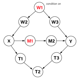
Figure 4: The demonstration for the d-separation. W1 and M1 are conditioned, which block all possible way from $X\rightarrow Y$. Therefore, X,Y are d-separated.

Two sets of nodes $X$ and $Y$ are d-separated by a set of nodes $Z$ if all of the paths between any node in $X$ and any node in $Y$ are blocked by $Z$. In Fig. 4, we provide an example to illustrate d-separation. If $X$ is the cause, $Y$ is the effect. The other node is confounding. If W1/W2/W3 and M1/M2 are conditioned on, $X$ and $Y$ are d-separated. If T2 is conditioned on, $X$ and $Y$ are not d-separated because the relationship between $X$ and $Y$ could be found by intervening T2. If both T1 and T2 are conditioned on, $X$ and $Y$ are d-separated because T1 blocks the information path at the bottom of the figure. This concept explains why $X\rightarrow M1\rightarrow M2\rightarrow Y$ is causal association and $X\rightarrow W1\rightarrow W2\rightarrow W3\rightarrow Y$, $X\rightarrow T1\rightarrow T2\rightarrow T3\rightarrow Y$ are non-causal associations.

2.4.2 Intervention

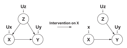
Figure 5: After the intervention on $X=x$, the edge from $Z\rightarrow X$ should be deleted.

We use $do(X=x)$ to represent intervention, $P(Y=y|do(X=x))$ represents the probability of $Y=y$ when making $X=x$. In the graphical model, one edge is deleted to represent the intervention on a particular node. From Fig.5, two invariant equations can be formulated by,

$$P_{m}(Y=y|Z=z,X=x)=P(Y=y|Z=z,X=x)$$ (6)

$$P_{m}(Z=z)=P(Z=z)$$

$Z$ and $X$ are d-separated after the modification, indicating that,

$$P_{m}(Z=z|X=x)=P_{m}(Z=z)=P(Z=z)$$ (7)

Therefore,

$$P(Y=y|do(X=x))=P_{m}(Y=y|X=x)$$ (8)

$$=\sum_{z}{P_{m}(Y=y|X=x,Z=z)P_{m}(Z=z|X=x)}$$

$$=\sum_{z}{P_{m}(Y=y|X=x,Z=z)P_{m}(Z=z)}$$

Finally, the causal effect formula before intervention can be obtained using the relationship of invariance,

$$P(Y=y|do(X=x))=\sum_{z}P(Y=y|X=x,Z=z)P(Z=z)$$ (9)

This formula is called the adjustment formula, calculating the relationship between $X$ and $Y$ For every value of $Z$.

Consider the example in Table.1 and the causal graph in Fig.5. $X=A/B$ donates to patients who take the drug A/B. $Z=Mild/Severe$ donates the level of illness. $Y$ donates the death rate.
The effect of taking the drug A:

$$E[Y|do(X=A)]=\frac{1450}{2050}(0.15)+\frac{600}{2050}(0.30)\approx 0.194$$ (10)

The effect of taking the drug B:

$$E[Y|do(X=B)]=\frac{1450}{2050}(0.10)+\frac{600}{2050}(0.20)\approx 0.129$$ (11)

The result indicates that treatment B has a better effect which is contradictory to the statistical results.

2.4.3 Backdoor criterion

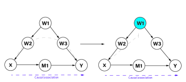
Figure 6: The example of the backdoor adjustment. The second line in Equ.12: W is a sufficient adjustment set, blocking all backdoor paths, only reserving the causation $X\rightarrow Y$. Third line in Equ.12: $do(X)$ blocks all T’s parents.

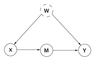
Figure 7: The example of the frontdoor adjustment. Typically, we do twice backdoor adjustments. Firstly, from $X\rightarrow M$, there is no backdoor path. Secondly, from $M\rightarrow Y$, T block the backdoor path $M\leftarrow X\leftarrow W\rightarrow Y$. Therefore, the final equation is defined in step 3.

$W$ is said to satisfy the backdoor criterion about $(X,Y)$, if $W$:

• blocks all paths between $X$ and $Y$.

• keeps the same directed paths from $X\rightarrow Y$.

• does not produce a new path.

Backdoor adjustment: if $W$ satisfies the backdoor criterion, then ATE (Average Treatment Effect) is identified.

$$P(y\mid do(X)) =\sum_{w}P(y\mid do(X),w)P(w\mid do(X))$$ (12)

$$=\sum_{w}P(y\mid X,w)P(w\mid do(X))$$

$$=\sum_{w}P(y\mid X,w)P(w)$$

2.4.4 Frontdoor criterion

$W$ is said to satisfy the backdoor criterion about $(X,Y)$, if:

• $W$ blocks all possible directed path from $X\rightarrow Y$.

• There is no backdoor path from $X\rightarrow W$

• All possible paths from $W\rightarrow Y$ are blocked by $X$.

Frontdoor adjustment:

• X on M: $P(m\mid do(x))=P(m\mid x)$

• M on Y: $P(y\mid do(m))=\sum_{x}P(y\mid m,x)P(x)$

• X on Y: $P(y\mid do(x))=\sum_{m}P(m\mid do(x))P(y\mid do(m))=\sum_{m}P(m\mid x)\sum_{x^{\prime}}P\left(y\mid m,x^{\prime}\right)P\left(x^{\prime}\right)$

2.4.5 Intermediate Effect

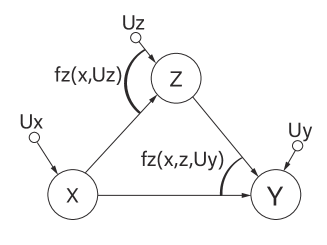
Figure 8: The mediation model without confounding.

In a causal model, a classical intermediate problem can be defined as:

$$x=f_{X}\left(U_{X}\right),z=f_{Z}\left(x,U_{Z}\right),y=f_{Y}\left(x,z,U_{Y}\right)$$ (13)

where $X$ donates treatment, $Z$ donates mediator, $Y$ donates outcome. $f_{X},f_{Z},f_{Y}$ are any function. $U_{X},U_{Z},U_{Y}$ are background variables (see. Fig.8). Based on this, the effect is analyzed by the intervention as follows,
Average Treatment Effect:

$$ATE =E[Y_{1}]-E[Y_{0}]$$ (14)

$$=E[Y\mid do(X=1)]-E[Y\mid do(X=0)]]$$

Controlled Direct Effect:

$$CDE(z)=E\left[Y_{1,Z}-Y_{0,Z}\right]$$ (15)

$$=E[Y\mid do(X=1,Z=z)]-E[Y\mid do(X=0,Z=z)]$$

Natural Direct Effect:

$$NDE=E\left[Y_{1,Z_{0}}-Y_{0,Z_{0}}\right]$$ (16)

Natural Indirect Effect:

$$NIE=E\left[Y_{0,Z_{1}}-Y_{0,Z_{0}}\right]$$ (17)

Total Direct Effect:

$$TDE=E\left[Y_{1,Z_{1}}-Y_{0,Z_{1}}\right]$$ (18)

Total Indirect Effect:

$$TIE=E\left[Y_{1,Z_{1}}-Y_{1,Z_{0}}\right]$$ (19)

Figure 9: The general workflow for causal representation learning in vision.

3 Causal Representation Learning in Vision

In this section, we introduce recent advances of CRL in theoretical works and practical works.

3.1 Theoretical Work

Traditional machine learning methods attempt to minimize the empirical risk (ERM). However, these methods can not be generalized to the unseen domain. Moreover, ERM is often over-parameterized, resulting in the discovery of spurious correlations. Based on the concept of causal inference, invariant risk minimizationd1-irm1 is introduced to solve the problems above. Consider a data representation $\Phi:\mathcal{X}\rightarrow\mathcal{H}$. we desire an invariant predictor across the environment $w\circ\Phi$. If there exists a predictor $w:\mathcal{H}\rightarrow\mathcal{Y}$ achieve optimal performance in every environment $\mathcal{E}_{\mathrm{tr}}$ such that $w\in\underset{\bar{w}:\mathcal{H}\rightarrow\mathcal{Y}}{\arg\min}R^{e}(\bar{w}\circ\Phi)$. Therefore, the constrained optimization problem is defined as:

$$\begin{array}[]{ll}\min_{\begin{subarray}{c}\Phi:\mathcal{X}\rightarrow\mathcal{H}\\ w:\mathcal{H}\rightarrow\mathcal{Y}\end{subarray}}&\sum_{e\in\mathcal{E}_{\mathrm{tr}}}R^{e}(w\circ\Phi)\\ \text{ subject to }&w\in\underset{\bar{w}:\mathcal{H}\rightarrow\mathcal{Y}}{\arg\min}R^{e}(\bar{w}\circ\Phi),\text{ for all }e\in\mathcal{E}_{\mathrm{tr}}\end{array}$$ (20)

To solve it via gradient descent method, an alternative penalty term is proposed,

$$\min_{\Phi:\mathcal{X}\rightarrow\mathcal{Y}}\sum_{e\in\mathcal{E}_{\mathrm{tr}}}R^{e}(\Phi)+\lambda\cdot\left\|\nabla_{w\mid w=1.0}R^{e}(w\cdot\Phi)\right\|^{2}$$ (21)

where $\mathrm{D}$ measures the risk when changing the environment, $\lambda\in[0,\infty)$ is a hyper-parameter balancing the ERM and the IRM. This paper only discussed the linear condition of $w$. In the colored MNIST synthetic task, the IRM method achieved 66.9$\%$ accuracy, whereas the ERM method could only achieve 17.1$\%$ accuracy, even lower than random guessing.

Despite the excellent performance on linear conditions, d1-irm2 proved that IRM can not find the optimal invariant predictor on most occasions and even suffer from a catastrophic failure in a particular condition. This paper first introduced and analyzed the non-linear scene. d1-irm3 deeply discussed the limitation of the IRM and proved that the IRM prefers an invariant predictor with worse o.o.d generalization. Moreover, the invariant loses its effect when using IRM on empirical samples rather than the population distributions. To address the problem that the IRM fails in the non-linear condition, d1-irm4 utilized the Bayesian inference to diminish the over-fitting problem and tricks like ELBO and reparameterization to accelerate convergence speed. d1-irm6 proposed sparse IRM to prevent the spurious correlation leaking to sub-models. On the dataset side, d1-irm5 proposed a Heterogeneous Risk Minimization (HRM) structure to address the mixture of multi-source data without a source label. Based on this work, d1-irm8 extended to kernel space, enhancing the ability to deal with more complex data and invariant relationships. d1-irm7 thought that the IRM method could not deal with the relationship between input and output in different domains. Therefore, d1-irm7 tried to modify the parameters to make the model robust when domain shifting based on mate-learning structure.

IRM method also mutually benefited from another theory. li2022invariant combined information bottleneck with IRM for domain adaptation. The loss is designed in a mutual information expression, whose structure is similar to the IRM.

Task	Performance Improvement over 2nd Model
Scene Graph Generationtang2020unbiased	Predicate Classification	Scene Graph Classification	Scene Graph Detection
	51.1%	56.4%	31.3%
	Zero-Shot Relationship Retrieval	Sentence-to-Graph Retrieval
	25.0%	33.7%
Image Captioningf8	Karpathy Splitkarpathy2015deep 5 Captions	Karpathy Split Whole Set	MS-COCOlin2014microsoft
	0.250%	1.55%	1.02%
Attention Mechanismf10	CNN-Based NICOhe2019nico	CNN-Based ImageNet-9deng2009imagenet	CNN-Based ImageNet-A
	8.72%	1.15%	8.33%
	ViT-Based NICO	ViT-Based ImageNet-9	ViT-Based ImageNet-A
	8.08%	2.78%	12.7%
Few-shot Learningf14	miniImageNet	tieredImageNet
	2.40%	0.94%
Long-tailed Classificationf13	LVIS V1.0gupta2019lvis val set	ImageNet-LT	LVIS V0.5 val set
	29.2%	17.3%	19.1%
	LVIS V0.5 eval test server
	18.8%
Incremental Learningf12	CIFAR-100cifar100	ImageNet-Sub	ImageNet-Full
	6.17%	4.76%	3.49%
Image Recognitionwang2020visual	MS-COCO	Open Imageskuznetsova2020open	VQA2.0 testantol2015vqa
	1.41%	1.09%	0.560%
Visual Groundingf5	RefCOCOkazemzadeh2014referitgame	RefCOCO+	RefCOCOg
	2.09%	2.36%	1.77%
	ReferIt Game	Flickr30K Entitiesplummer2015flickr30k
	1.14%	0.36%
Weakly-Supervised Learningf15	PASCAL VOC 2012pascal-voc-2012	MSCOCO
	1.84%	2.45%

Table 2: The performance improvement table for causal representation learning in practical works. Most of the works are plug-and-play and robust to other downstream tasks with only a few costs in total parameters.

3.2 Practical Work

Feature understanding and transfer learning are two specific research applications in CRL. Confounders are common in vision datasets, which mislead the machine model into catching the bad relationship. Research in feature understanding in CRL attempts to build the SCM and intervene in the node to discover the causal relationship. For transfer learning, statistical methods suffer from the o.o.d data. Discovering the causal or avoiding the adaptation risk reduce the complexity of training a new transfer learning algorithm and improve performance. This section will present the recent CRL advances in feature understanding and transfer learning.

3.2.1 Feature understanding

In object detection tasks, the highly correlated objects tend to occur in the same image (e.g. the chair and human, because people could sit on the chair instead of commensalism). VC R-CNNwang2020visual thought that observational bias made the model ignore the common causal relationship. They introduced an intervention (confounder dictionary) to measure the true causal effect.

In scene graph generation, tang2020unbiased compared the counterfactual scene and factual scene, using a Total Direct Effect (TDE) analysis framework to remove the bias in training. f9 proposed Align-RCNN to discover the feature relationship and concatenate those features dynamically.

In visual grounding (visual language tasks), the location of the target bounding box highly depends on the query instead of causal reasoning. f5 proposed a plug-and-play framework Referring Expression Deconfounder (RED), to make the backdoor adjustment to find the causal relationship between images and sentences.

In image captioning (visual language tasks), f8 thought that the pre-training model contains the confounder. The authors introduced the backdoor adjustment to deconfound the bias. Few-shot learningwang2020generalizing also requires the pre-training model. Similarly, f14 proposed three solutions, including feature-wise adjustment, class-wise adjustment, and class-wise adjustment. These operations do not need to modify the backbone and could be applied easily in zero-shot learning, meta-learninghospedales2021meta etc.

In the attention mechanism, most models worked well due to the i.i.d of the data. However, the o.o.d data degrades the performance when using attention. f10 proposed Casual Attention Module (Caam) on original CBAM-based CNNwoo2018cbam and ViTdosovitskiy2020image . This method utilized the IRM and adversarial traininggoodfellow2020generative with a partitioned dataset to discover confounding factor characteristics.

In feature (disentanglement) representation learning, the classical work simCLRchen2020simple proposed a Self-Supervised Learning (SSL), using a contrastive objective method to recognize similar images. However, the generalization performance and the interpretability are poor. f7 introduced Iterative Partition-based Invariant Risk Minimization (IP-IRM), combining feature disentanglement (data partition) and IRM. This method could discover the critical causal representation for classification tasks. f11 proposed a counterfactual generation framework for zero-shot learning taskslarochelle2008zero based on counterfactual faithfulness theorem. It designed a two-element classifier, disentangling the feature in class and sample.

In incremental learningmasana2020class , f12 used causal-effect theory to explain the forget and anti-forget. It designed models for distilling the causal effect of data, colliding effect, and removing SGD momentumsutskever2013importance (optimizer) effect of guaranteeing the effectiveness of introducing new data to learn. The interference of the SGD momentum also occurs in long-tailed classification because the update direction of SGD contains the information on data distribution. f13 designed a multi-head normalized classifier in training and made counterfactual TDE inference in testing to remove the excessive tendency for head class.

In weakly-supervised learningzhou2018brief for semantic segmentation, the problems often occur in pseudo-masks, for example, object ambiguity, incomplete background, and incomplete foreground. f15 introduced a causal intervention——blocking the connection between context prior and images to remove the fake association between label and images. f15 proposed a context adjustment for the unknown context prior, that is, using a class-specific average mask to approximately constructing a confounder set. chen2022c proposed a category causality chain and an anatomy-causality chain to solve the ambiguous boundary and co-occurrence problems in medical image segmentation.

3.2.2 Transfer learning

One of the popular research directions in transfer learning is domain adaptation. subbaswamy2020spec defined invariance specification: a 2-tuple $\langle\mathcal{P},\mathbf{M}\rangle$, where $\mathcal{P}$ donates graphical representation, $\mathbf{M}$ donates a group of variable (control the data from different environments). If an invariance spec is found, we could get a stable representation such that the model can be applied to the target domain. Similarly, d2-domain1 considered domain adaptation as an inference problem, constructing a DAG and solving it by Bayesian inference.

In image-to-image translation, d2-domain2 concluded a DAG and developed an important reweighting-based learning method. This method can automatically select the images and perform translation simultaneously.

In general, transfer learning, kunzel2018transfer introduced the new problem of transfer learning for estimating heterogeneous treatment effects and developed several methods (e.g. Y-Learner). rojas2018invariant proposed invariant models for transfer learning. zhang2017transfer utilized a causal approach to Multi-Armed Bandits in reinforcement learning.magliacane2018domain exploited causal inference to predict invariant conditional distribution in domain adaptation without prior knowledge of the causal graph and the type of interventions.

4 Future Work on Medical Image Analysis

Medical image analysis is a high-risk task, significantly requiring an explainable framework so that doctors and patients can rely on the diagnosis. The current works still lack interpretability and are treated as a black box. Causal representation learning is a promising learning paradigm for medical image analysis. In this section, we mention some prospective research directions.

4.1 Attention mechanism

Attention mechanism is widely applied in medical image analysis, and has shown promising results in lots of datasets and tasksatt1 att2 att3 att4 att5 att6 , especially for pure attention model (e.g. ViTdosovitskiy2020image , Swin-Transformerliu2021swin , Swin-UNetcao2021swin ). The attention mechanism will bring interpretability to the model. For example, in organ segmentation (e.g. cardiac, brain), attention could highlight the features of a region and suppress other noisy parts. However, the attention mechanism suffers from the data distribution shift (CNN-based attention) and the small scale of datasets (Transformer based). gonccalves2022survey shown that the results are noisy on some datasets, even for the cases of attention mechanisms. The causal attention module (Caam)tang2020unbiased is a promising method to solve this problem without changing the original framework.

4.2 Deconfounded optimizer

Most of the works have various settings of the optimizer, and the performance will be damaged if we change to another optimizer. As f12 f13 mentioned above, the optimizer (e.g. SGD momentum) can be a confounder in incremental learning and long-tailed classification. The design of a multi-head normalized classifier and counterfactual TDE inference could be a solution in the medical field.

4.3 Domain adaptation/generalization

The data distribution shift problem would decrease the performance of the original model due to the various sources from different hospitals. Recently, domain adaptationda1 da2 da3 da4 da5 da6 and domain generalizationdg1 dg2 dg3 dg4 dg5 techniques increased a great deal of accuracy (from $\approx 10\%$ to $\approx 70\%$ in these tasks. However, the model must be trained again when adding a new source for adaptation, and the tricks for domain generalization heavily depend on data pre-processing. Additionally, the performance ($\approx 70\%$) still can not be trusted and applied in clinical application. The series works of IRM d1-irm1 provide a new general solution for domain adaptation/generalization problems.

4.4 Feature disentanglement

Feature disentanglement attempts to desperate independent feature to make the model explainable. Specifically, classical feature disentanglement methods utilized the Variational Autoencodervae or GANgoodfellow2020generative with a restriction in different channels (e.g. minimize mutual information) to disentangle the high-level semantic representation. In domain adaptation, dis1 aimed to find the domain-specific feature and the domain invariant feature to make the model robust. In multi-task learning, dis2 proposed a dual-stream network to share the common feature in latent space. dis3 utilized a VAE to learn a multi-channel spatial representation of the anatomy. However, the restriction for disentanglement is still loose and lacks interpretability in the current work. We could refer to the concept of IP-IRMf7 to discover the causal representation of medical images.

4.5 Class imbalance learning

The solution to the class imbalance problem traditionally relies on the data pre-processing (e.g. oversamplingkotsiantis2006handling , re-weightingzhang2021learning etc.). But, we can not know the data distribution before training. Additionally, the trick, like re-weighting, will lead the head categories under-fitted. We could refer to f13 to invent a multi-head normalized classifier in training and make counterfactual TDE inference in testing to solve the long-tailed problem.

5 Conclusion and Prospect

This paper reviewed the development of causal representation learning from concept to application. Firstly, we introduce the basic knowledge of causal inference. Secondly, we analyze the theoretical works on IRM and practical works on feature understanding and transfer learning. The existing method shows promising results on benchmark datasets (the performance upgraded over 3-5$\%$ in many areas). Most of the works will not increase the complexity or parameter of the model (with a simple intervention or adjustment), but they are very effective and robust in different tasks. Finally, we also mention some future research directions in general CRL as follows:

• A well-defined causal graph is essential. However, some scenes, like anomaly detection, are very complicated. The performance of causal inference is sensitive to the causal graph.

• The suitable approximation of operation (intervention, backdoor/frontdoor adjustment) on a node in the causal graph is hard to design.

• Although causal inference is a promising way toward an explainable AI, a complete theory is required with mathematics definition.

• We should explore the effect of causal representation learning in downstream applications or tasks (e.g. medical image analysis, low-level vision, etc.)

References

- (1) D. E. Geer Jr, “Correlation is not causation,” IEEE Security & Privacy, vol. 9, no. 2, pp. 93–94, 2011.
- (2) C. H. Wagner, “Simpson’s paradox in real life,” The American Statistician, vol. 36, no. 1, pp. 46–48, 1982.
- (3) J. Pearl, “Causal inference in statistics: An overview,” Statistics surveys, vol. 3, pp. 96–146, 2009.
- (4) I. Shpitser and J. Pearl, “Complete identification methods for the causal hierarchy,” Journal of Machine Learning Research, vol. 9, pp. 1941–1979, 2008.
- (5) J. Pearl, Causality. Cambridge university press, 2009.
- (6) J. Splawa-Neyman, D. M. Dabrowska, and T. Speed, “On the application of probability theory to agricultural experiments. essay on principles. section 9.” Statistical Science, pp. 465–472, 1990.
- (7) D. B. Rubin, “Estimating causal effects of treatments in randomized and nonrandomized studies.” Journal of educational Psychology, vol. 66, no. 5, p. 688, 1974.
- (8) J. Pearl, Probabilistic reasoning in intelligent systems: networks of plausible inference. Morgan kaufmann, 1988.
- (9) P. Spirtes, C. N. Glymour, R. Scheines, and D. Heckerman, Causation, prediction, and search. MIT press, 2000.
- (10) J. Pearl et al., “Models, reasoning and inference,” Cambridge, UK: CambridgeUniversityPress, vol. 19, no. 2, 2000.
- (11) J. Pearl, “A probabilistic calculus of actions,” in Uncertainty Proceedings 1994. Elsevier, 1994, pp. 454–462.
- (12) L. Yao, Z. Chu, S. Li, Y. Li, J. Gao, and A. Zhang, “A survey on causal inference,” ACM Transactions on Knowledge Discovery from Data (TKDD), vol. 15, no. 5, pp. 1–46, 2021.
- (13) G. W. Imbens and D. B. Rubin, Causal inference in statistics, social, and biomedical sciences. Cambridge University Press, 2015.
- (14) M. Gangl, “Causal inference in sociological research,” Annual review of sociology, vol. 36, pp. 21–47, 2010.
- (15) E. Bareinboim, J. D. Correa, D. Ibeling, and T. Icard, “On pearl’s hierarchy and the foundations of causal inference,” in Probabilistic and Causal Inference: The Works of Judea Pearl, 2022, pp. 507–556.
- (16) W. Zhang, R. Ramezani, and A. Naeim, “Causal inference in medicine and in health policy, a summary,” arXiv preprint arXiv:2105.04655, 2021.
- (17) M. Harel, “Lmu, cmsi 498: your window into the cromulent world of cognitive systems,” 2019.
- (18) K. He, X. Zhang, S. Ren, and J. Sun, “Deep residual learning for image recognition,” in Proceedings of the IEEE conference on computer vision and pattern recognition, 2016, pp. 770–778.
- (19) A. Vaswani, N. Shazeer, N. Parmar, J. Uszkoreit, L. Jones, A. N. Gomez, Ł. Kaiser, and I. Polosukhin, “Attention is all you need,” Advances in neural information processing systems, vol. 30, 2017.
- (20) D. Ren, W. Zuo, Q. Hu, P. Zhu, and D. Meng, “Progressive image deraining networks: A better and simpler baseline,” in Proceedings of the IEEE/CVF Conference on Computer Vision and Pattern Recognition, 2019, pp. 3937–3946.
- (21) S. Zheng, C. Lu, Y. Wu, and G. Gupta, “Sapnet: Segmentation-aware progressive network for perceptual contrastive deraining,” in Proceedings of the IEEE/CVF Winter Conference on Applications of Computer Vision, 2022, pp. 52–62.
- (22) K. Jiang, Z. Wang, P. Yi, C. Chen, B. Huang, Y. Luo, J. Ma, and J. Jiang, “Multi-scale progressive fusion network for single image deraining,” in Proceedings of the IEEE/CVF conference on computer vision and pattern recognition, 2020, pp. 8346–8355.
- (23) Z. Cui, K. Li, L. Gu, S. Su, P. Gao, Z. Jiang, Y. Qiao, and T. Harada, “You only need 90k parameters to adapt light: A light weight transformer for image enhancement and exposure correction.”
- (24) C. R. Qi, H. Su, K. Mo, and L. J. Guibas, “Pointnet: Deep learning on point sets for 3d classification and segmentation,” in Proceedings of the IEEE conference on computer vision and pattern recognition, 2017, pp. 652–660.
- (25) C. R. Qi, L. Yi, H. Su, and L. J. Guibas, “Pointnet++: Deep hierarchical feature learning on point sets in a metric space,” Advances in neural information processing systems, vol. 30, 2017.
- (26) B. Schölkopf, F. Locatello, S. Bauer, N. R. Ke, N. Kalchbrenner, A. Goyal, and Y. Bengio, “Toward causal representation learning,” Proceedings of the IEEE, vol. 109, no. 5, pp. 612–634, 2021.
- (27) C.-X. Ren, X.-L. Xu, and H. Yan, “Generalized conditional domain adaptation: A causal perspective with low-rank translators,” IEEE transactions on cybernetics, vol. 50, no. 2, pp. 821–834, 2018.
- (28) S. Basu, X. Li, and G. Michailidis, “Low rank and structured modeling of high-dimensional vector autoregressions,” IEEE Transactions on Signal Processing, vol. 67, no. 5, pp. 1207–1222, 2019.
- (29) F. Xie, R. Cai, B. Huang, C. Glymour, Z. Hao, and K. Zhang, “Generalized independent noise condition for estimating latent variable causal graphs,” Advances in Neural Information Processing Systems, vol. 33, pp. 14 891–14 902, 2020.
- (30) ——, “Generalized independent noise condition for estimating linear non-gaussian latent variable graphs,” 2020.
- (31) M. Arjovsky, L. Bottou, I. Gulrajani, and D. Lopez-Paz, “Invariant risk minimization,” arXiv preprint arXiv:1907.02893, 2019.
- (32) E. Rosenfeld, P. Ravikumar, and A. Risteski, “The risks of invariant risk minimization,” arXiv preprint arXiv:2010.05761, 2020.
- (33) P. Kamath, A. Tangella, D. Sutherland, and N. Srebro, “Does invariant risk minimization capture invariance?” in International Conference on Artificial Intelligence and Statistics. PMLR, 2021, pp. 4069–4077.
- (34) Y. Lin, H. Dong, H. Wang, and T. Zhang, “Bayesian invariant risk minimization,” in Proceedings of the IEEE/CVF Conference on Computer Vision and Pattern Recognition, 2022, pp. 16 021–16 030.
- (35) J. Liu, Z. Hu, P. Cui, B. Li, and Z. Shen, “Heterogeneous risk minimization,” in International Conference on Machine Learning. PMLR, 2021, pp. 6804–6814.
- (36) X. Zhou, Y. Lin, W. Zhang, and T. Zhang, “Sparse invariant risk minimization,” in International Conference on Machine Learning. PMLR, 2022, pp. 27 222–27 244.
- (37) M. Zhang, H. Marklund, N. Dhawan, A. Gupta, S. Levine, and C. Finn, “Adaptive risk minimization: Learning to adapt to domain shift,” Advances in Neural Information Processing Systems, vol. 34, pp. 23 664–23 678, 2021.
- (38) J. Liu, Z. Hu, P. Cui, B. Li, and Z. Shen, “Kernelized heterogeneous risk minimization,” arXiv preprint arXiv:2110.12425, 2021.
- (39) T. Wang, J. Huang, H. Zhang, and Q. Sun, “Visual commonsense r-cnn,” in Proceedings of the IEEE/CVF Conference on Computer Vision and Pattern Recognition, 2020, pp. 10 760–10 770.
- (40) K. Tang, Y. Niu, J. Huang, J. Shi, and H. Zhang, “Unbiased scene graph generation from biased training,” in Proceedings of the IEEE/CVF conference on computer vision and pattern recognition, 2020, pp. 3716–3725.
- (41) J. Huang, Y. Qin, J. Qi, Q. Sun, and H. Zhang, “Deconfounded visual grounding,” in Proceedings of the AAAI Conference on Artificial Intelligence, vol. 36, no. 1, 2022, pp. 998–1006.
- (42) M. Li, F. Feng, H. Zhang, X. He, F. Zhu, and T.-S. Chua, “Learning to imagine: Integrating counterfactual thinking in neural discrete reasoning,” in Proceedings of the 60th Annual Meeting of the Association for Computational Linguistics (Volume 1: Long Papers), 2022, pp. 57–69.
- (43) T. Wang, Z. Yue, J. Huang, Q. Sun, and H. Zhang, “Self-supervised learning disentangled group representation as feature,” Advances in Neural Information Processing Systems, vol. 34, pp. 18 225–18 240, 2021.
- (44) X. Yang, H. Zhang, and J. Cai, “Deconfounded image captioning: A causal retrospect,” IEEE Transactions on Pattern Analysis and Machine Intelligence, 2021.
- (45) M. Tajrobehkar, K. Tang, H. Zhang, and J.-H. Lim, “Align r-cnn: A pairwise head network for visual relationship detection,” IEEE Transactions on Multimedia, vol. 24, pp. 1266–1276, 2021.
- (46) T. Wang, C. Zhou, Q. Sun, and H. Zhang, “Causal attention for unbiased visual recognition,” in Proceedings of the IEEE/CVF International Conference on Computer Vision, 2021, pp. 3091–3100.
- (47) Z. Yue, T. Wang, Q. Sun, X.-S. Hua, and H. Zhang, “Counterfactual zero-shot and open-set visual recognition,” in Proceedings of the IEEE/CVF Conference on Computer Vision and Pattern Recognition, 2021, pp. 15 404–15 414.
- (48) X. Hu, K. Tang, C. Miao, X.-S. Hua, and H. Zhang, “Distilling causal effect of data in class-incremental learning,” in Proceedings of the IEEE/CVF Conference on Computer Vision and Pattern Recognition, 2021, pp. 3957–3966.
- (49) K. Tang, J. Huang, and H. Zhang, “Long-tailed classification by keeping the good and removing the bad momentum causal effect,” Advances in Neural Information Processing Systems, vol. 33, pp. 1513–1524, 2020.
- (50) Z. Yue, H. Zhang, Q. Sun, and X.-S. Hua, “Interventional few-shot learning,” Advances in neural information processing systems, vol. 33, pp. 2734–2746, 2020.
- (51) D. Zhang, H. Zhang, J. Tang, X.-S. Hua, and Q. Sun, “Causal intervention for weakly-supervised semantic segmentation,” Advances in Neural Information Processing Systems, vol. 33, pp. 655–666, 2020.
- (52) K. Zhang, M. Gong, P. Stojanov, B. Huang, Q. Liu, and C. Glymour, “Domain adaptation as a problem of inference on graphical models,” Advances in Neural Information Processing Systems, vol. 33, pp. 4965–4976, 2020.
- (53) S. Xie, M. Gong, Y. Xu, and K. Zhang, “Unaligned image-to-image translation by learning to reweight,” in Proceedings of the IEEE/CVF International Conference on Computer Vision, 2021, pp. 14 174–14 184.
- (54) B. Huang, K. Zhang, M. Gong, and C. Glymour, “Causal discovery and forecasting in nonstationary environments with state-space models,” in International conference on machine learning. PMLR, 2019, pp. 2901–2910.
- (55) A. Subbaswamy and S. Saria, “I-spec: An end-to-end framework for learning transportable, shift-stable models,” arXiv preprint arXiv:2002.08948, 2020.
- (56) B. Huang, K. Zhang, J. Zhang, J. D. Ramsey, R. Sanchez-Romero, C. Glymour, and B. Schölkopf, “Causal discovery from heterogeneous/nonstationary data.” J. Mach. Learn. Res., vol. 21, no. 89, pp. 1–53, 2020.
- (57) B. Huang, F. Feng, C. Lu, S. Magliacane, and K. Zhang, “Adarl: What, where, and how to adapt in transfer reinforcement learning,” arXiv preprint arXiv:2107.02729, 2021.
- (58) D. C. Castro, I. Walker, and B. Glocker, “Causality matters in medical imaging,” Nature Communications, vol. 11, no. 1, pp. 1–10, 2020.
- (59) B. Neal, “Introduction to causal inference from a machine learning perspective,” Course Lecture Notes (draft), 2020.
- (60) B. Li, Y. Shen, Y. Wang, W. Zhu, D. Li, K. Keutzer, and H. Zhao, “Invariant information bottleneck for domain generalization,” in Proceedings of the AAAI Conference on Artificial Intelligence, vol. 36, no. 7, 2022, pp. 7399–7407.
- (61) A. Karpathy and L. Fei-Fei, “Deep visual-semantic alignments for generating image descriptions,” in Proceedings of the IEEE conference on computer vision and pattern recognition, 2015, pp. 3128–3137.
- (62) T.-Y. Lin, M. Maire, S. Belongie, J. Hays, P. Perona, D. Ramanan, P. Dollár, and C. L. Zitnick, “Microsoft coco: Common objects in context,” in European conference on computer vision. Springer, 2014, pp. 740–755.
- (63) Y. He, Z. Shen, and P. Cui, “Nico: A dataset towards non-iid image classification,” 2019.
- (64) J. Deng, W. Dong, R. Socher, L.-J. Li, K. Li, and L. Fei-Fei, “Imagenet: A large-scale hierarchical image database,” in 2009 IEEE conference on computer vision and pattern recognition. Ieee, 2009, pp. 248–255.
- (65) A. Gupta, P. Dollar, and R. Girshick, “Lvis: A dataset for large vocabulary instance segmentation,” in Proceedings of the IEEE/CVF conference on computer vision and pattern recognition, 2019, pp. 5356–5364.
- (66) A. Krizhevsky, V. Nair, and G. Hinton, “Cifar-100 (canadian institute for advanced research).” [Online]. Available: http://www.cs.toronto.edu/~kriz/cifar.html
- (67) A. Kuznetsova, H. Rom, N. Alldrin, J. Uijlings, I. Krasin, J. Pont-Tuset, S. Kamali, S. Popov, M. Malloci, A. Kolesnikov et al., “The open images dataset v4,” International Journal of Computer Vision, vol. 128, no. 7, pp. 1956–1981, 2020.
- (68) S. Antol, A. Agrawal, J. Lu, M. Mitchell, D. Batra, C. L. Zitnick, and D. Parikh, “Vqa: Visual question answering,” in Proceedings of the IEEE international conference on computer vision, 2015, pp. 2425–2433.
- (69) S. Kazemzadeh, V. Ordonez, M. Matten, and T. Berg, “Referitgame: Referring to objects in photographs of natural scenes,” in Proceedings of the 2014 conference on empirical methods in natural language processing (EMNLP), 2014, pp. 787–798.
- (70) B. A. Plummer, L. Wang, C. M. Cervantes, J. C. Caicedo, J. Hockenmaier, and S. Lazebnik, “Flickr30k entities: Collecting region-to-phrase correspondences for richer image-to-sentence models,” in Proceedings of the IEEE international conference on computer vision, 2015, pp. 2641–2649.
- (71) M. Everingham, L. Van Gool, C. K. I. Williams, J. Winn, and A. Zisserman, “The PASCAL Visual Object Classes Challenge 2012 (VOC2012) Results,” http://www.pascal-network.org/challenges/VOC/voc2012.
- (72) Y. Wang, Q. Yao, J. T. Kwok, and L. M. Ni, “Generalizing from a few examples: A survey on few-shot learning,” ACM computing surveys (csur), vol. 53, no. 3, pp. 1–34, 2020.
- (73) T. Hospedales, A. Antoniou, P. Micaelli, and A. Storkey, “Meta-learning in neural networks: A survey,” IEEE transactions on pattern analysis and machine intelligence, vol. 44, no. 9, pp. 5149–5169, 2021.
- (74) S. Woo, J. Park, J.-Y. Lee, and I. S. Kweon, “Cbam: Convolutional block attention module,” in Proceedings of the European conference on computer vision (ECCV), 2018, pp. 3–19.
- (75) A. Dosovitskiy, L. Beyer, A. Kolesnikov, D. Weissenborn, X. Zhai, T. Unterthiner, M. Dehghani, M. Minderer, G. Heigold, S. Gelly et al., “An image is worth 16x16 words: Transformers for image recognition at scale,” arXiv preprint arXiv:2010.11929, 2020.
- (76) I. Goodfellow, J. Pouget-Abadie, M. Mirza, B. Xu, D. Warde-Farley, S. Ozair, A. Courville, and Y. Bengio, “Generative adversarial networks,” Communications of the ACM, vol. 63, no. 11, pp. 139–144, 2020.
- (77) T. Chen, S. Kornblith, M. Norouzi, and G. Hinton, “A simple framework for contrastive learning of visual representations,” in International conference on machine learning. PMLR, 2020, pp. 1597–1607.
- (78) H. Larochelle, D. Erhan, and Y. Bengio, “Zero-data learning of new tasks.” in AAAI, vol. 1, no. 2, 2008, p. 3.
- (79) M. Masana, X. Liu, B. Twardowski, M. Menta, A. D. Bagdanov, and J. van de Weijer, “Class-incremental learning: survey and performance evaluation on image classification,” arXiv preprint arXiv:2010.15277, 2020.
- (80) I. Sutskever, J. Martens, G. Dahl, and G. Hinton, “On the importance of initialization and momentum in deep learning,” in International conference on machine learning. PMLR, 2013, pp. 1139–1147.
- (81) Z.-H. Zhou, “A brief introduction to weakly supervised learning,” National science review, vol. 5, no. 1, pp. 44–53, 2018.
- (82) Z. Chen, Z. Tian, J. Zhu, C. Li, and S. Du, “C-cam: Causal cam for weakly supervised semantic segmentation on medical image,” in Proceedings of the IEEE/CVF Conference on Computer Vision and Pattern Recognition, 2022, pp. 11 676–11 685.
- (83) S. R. Künzel, B. C. Stadie, N. Vemuri, V. Ramakrishnan, J. S. Sekhon, and P. Abbeel, “Transfer learning for estimating causal effects using neural networks,” arXiv preprint arXiv:1808.07804, 2018.
- (84) M. Rojas-Carulla, B. Schölkopf, R. Turner, and J. Peters, “Invariant models for causal transfer learning,” The Journal of Machine Learning Research, vol. 19, no. 1, pp. 1309–1342, 2018.
- (85) J. Zhang and E. Bareinboim, “Transfer learning in multi-armed bandit: a causal approach,” in Proceedings of the 16th Conference on Autonomous Agents and MultiAgent Systems, 2017, pp. 1778–1780.
- (86) S. Magliacane, T. Van Ommen, T. Claassen, S. Bongers, P. Versteeg, and J. M. Mooij, “Domain adaptation by using causal inference to predict invariant conditional distributions,” Advances in neural information processing systems, vol. 31, 2018.
- (87) W. Zhu, L. Sun, J. Huang, L. Han, and D. Zhang, “Dual attention multi-instance deep learning for alzheimer’s disease diagnosis with structural mri,” IEEE Transactions on Medical Imaging, vol. 40, no. 9, pp. 2354–2366, 2021.
- (88) A. Sinha and J. Dolz, “Multi-scale self-guided attention for medical image segmentation,” IEEE journal of biomedical and health informatics, vol. 25, no. 1, pp. 121–130, 2020.
- (89) X. Wang, S. Han, Y. Chen, D. Gao, and N. Vasconcelos, “Volumetric attention for 3d medical image segmentation and detection,” in International conference on medical image computing and computer-assisted intervention. Springer, 2019, pp. 175–184.
- (90) N. Abraham and N. M. Khan, “A novel focal tversky loss function with improved attention u-net for lesion segmentation,” in 2019 IEEE 16th international symposium on biomedical imaging (ISBI 2019). IEEE, 2019, pp. 683–687.
- (91) R. Azad, M. Asadi-Aghbolaghi, M. Fathy, and S. Escalera, “Attention deeplabv3+: Multi-level context attention mechanism for skin lesion segmentation,” in European conference on computer vision. Springer, 2020, pp. 251–266.
- (92) C. Li, Y. Tan, W. Chen, X. Luo, Y. Gao, X. Jia, and Z. Wang, “Attention unet++: A nested attention-aware u-net for liver ct image segmentation,” in 2020 IEEE International Conference on Image Processing (ICIP). IEEE, 2020, pp. 345–349.
- (93) Z. Liu, Y. Lin, Y. Cao, H. Hu, Y. Wei, Z. Zhang, S. Lin, and B. Guo, “Swin transformer: Hierarchical vision transformer using shifted windows,” in Proceedings of the IEEE/CVF International Conference on Computer Vision, 2021, pp. 10 012–10 022.
- (94) H. Cao, Y. Wang, J. Chen, D. Jiang, X. Zhang, Q. Tian, and M. Wang, “Swin-unet: Unet-like pure transformer for medical image segmentation,” arXiv preprint arXiv:2105.05537, 2021.
- (95) T. Gonçalves, I. Rio-Torto, L. F. Teixeira, and J. S. Cardoso, “A survey on attention mechanisms for medical applications: are we moving towards better algorithms?” 2022.
- (96) F. Wu and X. Zhuang, “Cf distance: A new domain discrepancy metric and application to explicit domain adaptation for cross-modality cardiac image segmentation,” IEEE Transactions on Medical Imaging, vol. 39, no. 12, pp. 4274–4285, 2020.
- (97) C. Chen, Q. Dou, H. Chen, J. Qin, and P. A. Heng, “Unsupervised bidirectional cross-modality adaptation via deeply synergistic image and feature alignment for medical image segmentation,” IEEE transactions on medical imaging, vol. 39, no. 7, pp. 2494–2505, 2020.
- (98) Q. Dou, C. Ouyang, C. Chen, H. Chen, B. Glocker, X. Zhuang, and P.-A. Heng, “Pnp-adanet: Plug-and-play adversarial domain adaptation network at unpaired cross-modality cardiac segmentation,” IEEE Access, vol. 7, pp. 99 065–99 076, 2019.
- (99) Q. Dou, C. Ouyang, C. Chen, H. Chen, and P.-A. Heng, “Unsupervised cross-modality domain adaptation of convnets for biomedical image segmentations with adversarial loss,” arXiv preprint arXiv:1804.10916, 2018.
- (100) F. Wu and X. Zhuang, “Unsupervised domain adaptation with variational approximation for cardiac segmentation,” IEEE Transactions on Medical Imaging, vol. 40, no. 12, pp. 3555–3567, 2021.
- (101) M. Gu, S. Vesal, R. Kosti, and A. Maier, “Few-shot unsupervised domain adaptation for multi-modal cardiac image segmentation,” arXiv preprint arXiv:2201.12386, 2022.
- (102) Q. Liu, C. Chen, J. Qin, Q. Dou, and P.-A. Heng, “Feddg: Federated domain generalization on medical image segmentation via episodic learning in continuous frequency space,” in Proceedings of the IEEE/CVF Conference on Computer Vision and Pattern Recognition, 2021, pp. 1013–1023.
- (103) L. Zhang, X. Wang, D. Yang, T. Sanford, S. Harmon, B. Turkbey, B. J. Wood, H. Roth, A. Myronenko, D. Xu et al., “Generalizing deep learning for medical image segmentation to unseen domains via deep stacked transformation,” IEEE transactions on medical imaging, vol. 39, no. 7, pp. 2531–2540, 2020.
- (104) H. Li, Y. Wang, R. Wan, S. Wang, T.-Q. Li, and A. Kot, “Domain generalization for medical imaging classification with linear-dependency regularization,” Advances in Neural Information Processing Systems, vol. 33, pp. 3118–3129, 2020.
- (105) L. Li, V. A. Zimmer, W. Ding, F. Wu, L. Huang, J. A. Schnabel, and X. Zhuang, “Random style transfer based domain generalization networks integrating shape and spatial information,” in International Workshop on Statistical Atlases and Computational Models of the Heart. Springer, 2020, pp. 208–218.
- (106) L. Li, V. A. Zimmer, J. A. Schnabel, and X. Zhuang, “Atrialgeneral: Domain generalization for left atrial segmentation of multi-center lge mris,” in International Conference on Medical Image Computing and Computer-Assisted Intervention. Springer, 2021, pp. 557–566.
- (107) D. P. Kingma and M. Welling, “Auto-encoding variational bayes,” arXiv preprint arXiv:1312.6114, 2013.
- (108) C. Pei, F. Wu, L. Huang, and X. Zhuang, “Disentangle domain features for cross-modality cardiac image segmentation,” Medical Image Analysis, vol. 71, p. 102078, 2021.
- (109) H. Che, H. Jin, and H. Chen, “Learning robust representation for joint grading of ophthalmic diseases via adaptive curriculum and feature disentanglement,” in International Conference on Medical Image Computing and Computer-Assisted Intervention. Springer, 2022, pp. 523–533.
- (110) A. Chartsias, T. Joyce, G. Papanastasiou, S. Semple, M. Williams, D. E. Newby, R. Dharmakumar, and S. A. Tsaftaris, “Disentangled representation learning in cardiac image analysis,” Medical image analysis, vol. 58, p. 101535, 2019.
- (111) S. Kotsiantis, D. Kanellopoulos, P. Pintelas et al., “Handling imbalanced datasets: A review,” GESTS international transactions on computer science and engineering, vol. 30, no. 1, pp. 25–36, 2006.
- (112) Z. Zhang and T. Pfister, “Learning fast sample re-weighting without reward data,” in Proceedings of the IEEE/CVF International Conference on Computer Vision, 2021, pp. 725–734.