Flows For The Masses:
A multi-fluid non-linear perturbation theory for massive neutrinos

Abstract

Velocity dispersion of the massive neutrinos presents a daunting challenge for non-linear cosmological perturbation theory. We consider the neutrino population as a collection of non-linear fluids, each with uniform initial momentum, through an extension of the Time Renormalization Group perturbation theory. Employing recently-developed Fast Fourier Transform techniques, we accelerate our non-linear perturbation theory by more than two orders of magnitude, making it quick enough for practical use. After verifying that the neutrino mode-coupling integrals and power spectra converge, we show that our perturbation theory agrees with N-body neutrino simulations to within $10\%$ for neutrino fractions $\Omega_{\nu,0}h^{2}\leq 0.005$ up to wave numbers of $k=1~{}h/$Mpc, an accuracy consistent with $\leq 2.5\%$ errors in the neutrino mass determination. Non-linear growth represents a $>10\%$ correction to the neutrino power spectrum even for density fractions as low as $\Omega_{\nu,0}h^{2}=0.001$, demonstrating the limits of linear theory for accurate neutrino power spectrum predictions. Our code FlowsForTheMasses is avaliable online at github.com/upadhye/FlowsForTheMasses .

1 Introduction

Cosmic surveys are rapidly closing in on the sum of neutrino masses $\sum m_{\nu}$, one of the final unmeasured parameters of the Standard Model of particle physics. Joint analyses using restrictive assumptions about the dark energy find $95\%$ CL upper bounds on $\sum m_{\nu}$ ranging from $0.09$ eV to $0.14$ eV [1, 2, 3, 4], about twice the lower bound from neutrino oscillation experiments [5, 6]. Yet the case for considering larger neutrino masses remains compelling. Allowing a time-varying dark energy equation of state, or analyzing different combinations of cosmological data, can weaken the upper bound on the sum of neutrino masses to $\approx 0.5$ eV or larger [7, 8, 9]. Neutrinos and other hot dark matter may help resolve long-running tensions in the cosmic expansion rate [10, 11, 12, 13, 14], measures of the clustering amplitude [15, 16, 17], and laboratory oscillation experiments [18, 19, 20], though others cast doubt upon such resolutions [21, 22]. Independently of these tensions, constraints are weak on the distribution functions of muon, tau, and hypothetical sterile neutrinos, while substantial deviations from the Fermi-Dirac distribution can make larger-mass neutrinos consistent with observations [23, 24].

Neutrinos, especially those with larger masses, present several unique cosmic signatures which may allow for their definitive detection. They introduce a scale-dependence into the dark matter halo bias [25, 26, 27, 28]; a dipole distortion in galaxy cross-correlations due to their relative velocities [29, 30, 31, 32]; a long-range correlation in galactic rotation directions [33]; “wakes” caused by neutrinos coherently free-streaming past collapsed halos [34, 35]; non-Gaussianity due to their clustering in voids [36]; a suppression in mass accretion by dark matter halos [37]; and an environment-dependence of the halo mass function due to differential capture of neutrinos by halos [38]. Quantifying these effects requires accurate computations of the formation of large-scale structure in the non-linear regime.

Chief among the obstacles to such a computation is the large thermal velocity dispersion of the neutrino population, which requires that we follow its full six-dimensional phase space, rather than the three dimensions characterizing cold species such as the baryons. The most accurate approach is an N-body computer simulation realizing the cold dark matter (CDM) and baryons as a set of point particles, with neutrinos treated through either perturbation theory responding to non-linear CDM+baryon clustering [39, 40, 41, 42, 43, 44, 45, 46, 47] or as point particles themselves [48, 49, 50, 51, 52, 53, 54, 55, 56, 57, 58]. Since perturbation theory is more accurate for weakly-clustering neutrinos with high thermal velocities, while an N-body treatment more accurately captures non-linear neutrino clustering, hybrid simulations combine the two approaches, selectively realizing a low-velocity portion of the neutrino population as particles [59]. In the absence of a complete non-linear neutrino perturbation theory, N-body and hybrid techniques have provided the only accurate computations of the non-linear neutrino clustering power.

We present the first fully non-linear perturbative calculation of the massive neutrino power spectrum. Our theoretical advance represents the convergence of three distinct currents in cosmological perturbation theory: non-linear perturbation theory, multi-fluid treatments of hot dark matter, and Fast Fourier Transform (FFT) acceleration techniques. Firstly, in response to observations of the matter and galaxy power spectra pushing to ever-smaller length scales, non-linear perturbation theory was developed to extend the reach of cosmological perturbation theory [60, 61, 62, 63, 64, 65, 66, 67, 68, 69, 70]. The Time-Renormalization Group (Time-RG) perturbation theory of Refs. [68, 69] and the bispectrum of Ref. [71] are of particular interest to us here.

Secondly, Dupuy and Bernardeau formulated a multi-fluid linear perturbation theory for massive neutrinos [72, 73, 74]. The hot neutrino gas, with a thermal velocity dispersion described by a Fermi-Dirac distribution of momenta, is subdivided into bins, each characterized by a uniform initial velocity. Importantly, this theory is Lagrangian in momentum space, meaning that neutrinos cannot jump from one velocity bin to another, simplifying the theoretical description. Reference [45] developed a multi-fluid linear response calculation in which a non-relativistic version of this binned perturbation theory was used to track the response of massive neutrinos to the clustering of the cold dark matter (CDM) and baryons.

Thirdly, FFT techniques were applied by Refs. [75, 76, 77, 7] to reducing the computational expense of non-linear perturbation theory by orders of magnitude. By contrast to linear theory, non-linear perturbation theory couples different wave numbers. It quantifies these couplings through multi-dimensional mode-coupling integrals which represent the bulk of its computational cost. Time-RG perturbation theory is especially expensive due to requiring the computation of mode-coupling integrals at each time step. Its advantage is its ready applicability to multiple species which cluster differently and to expansion histories very different from that of the Einstein-de Sitter cosmology. Reference [7] used FFTs to accelerate Time-RG and the galaxy bias of Ref. [78], then applied them to a data analysis.

In this article, we construct an FFT-accelerated non-linear multi-fluid perturbation theory for massive neutrinos, which we call FlowsForTheMasses. We begin by extending Time-RG perturbation theory to a fluid with a spatially-uniform velocity $\vec{v}$. Rather than depending solely upon the wave number $k$, the linear multi-fluid theory has a preferred direction $\hat{v}$, with perturbations dependent upon both $k$ and $\hat{k}\cdot\hat{v}$, the cosine of the angle between the velocity and the Fourier vector. The bispectrum $B(\vec{k},\vec{q},\vec{p})$, or Fourier-transformed three-point correlation function, is an object of central importance in Time-RG. In the case of a non-zero velocity, the bipsectrum also gains a dependence upon the angles between its three wave vectors and the velocity. We generalize the bispectrum integrals of Time-RG, which quantify non-linear corrections to the power spectrum, to apply to a fluid with a uniform background velocity. Then we derive the equations of motion of these generalized bispectrum integrals, whose non-linear contribution, in turn, is sourced by generalized mode-coupling integrals.

Next, we proceed to a systematic study of these mode-coupling integrals. In ordinary Time-RG, assuming a power spectrum tracked using $N_{k}\sim 100$ wave number bins, the computation of a two-dimensional mode-coupling integral at each of the $N_{k}$ points involves a computational cost ${\mathcal{O}}(N_{k}^{3})$. In our extension to multi-fluid perturbation theory, the number of these mode-coupling integrals also grows as a high power of $N_{\mu}$, the number of angular modes which we use to track the dependence of perturbations upon the angle between $\vec{k}$ and $\vec{v}$. Thus FFT acceleration, which reduces the computational cost of a single mode-coupling integral from ${\mathcal{O}}(N_{k}^{3})$ to ${\mathcal{O}}(N_{k}\log N_{k})$, is essential to our method. After considerable algebra, we derive mode-coupling integrals that are percent-level accurate over our region of interest, and we use FFT acceleration to reduce their computational cost by a factor of four hundred.

Finally, we put our perturbation theory to the test against the hybrid neutrino N-body simulation of Ref. [79], which itself is based upon a multi-fluid treatment of the neutrinos. This hybrid simulation can track individual neutrino fluids, either using the multi-fluid linear response of Ref. [45], or by realizing them as massive particles, each beginning with a velocity $\vec{v}$ in addition to any velocity kicks it receives from the local gravitational potential. We confirm the accuracy of our perturbation theory, particularly at early times, $z\gtrsim 1$, and higher velocities, $v/c\gtrsim 0.2\%$. Our results accord with our intuition that non-linear perturbation theory will lose accuracy as the non-linear corrections come to dominate the power. Nevertheless, we find that even our fully perturbative computation agrees with simulations to $<10\%$ at $z=0$ for neutrino fractions up to $\Omega_{\nu,0}h^{2}=0.005$ and $k\leq 1~{}h/$Mpc.

High-velocity neutrinos are particularly difficult for N-body particle simulations. Firstly, they require small time steps, since they move quickly past collapsed structures which could deflect them. Secondly, momentum shells at higher $|\vec{p}|$ occupy more phase space volume, meaning that more particles are necessary in order to keep shot noise under control. Thus our work points the way to a hybrid multi-fluid non-linear-response simulation in which each neutrino fluid would be evolved linearly until its dimensionless power spectrum exceeded a predetermined threshold. Then it would be evolved non-linearly until the non-linear corrections themselves became a significant portion of the total power, at which point it could be converted into simulation particles. Our non-linear multi-fluid perturbation theory of massive neutrinos, when integrated into a hybrid simulation, promises several advantages:

1. Non-linear corrections make perturbative neutrino calculations more accurate.

2. Error in the perturbative calculation may be estimated using the ratio of non-linear corrections to the linear power.

3. Multi-fluid perturbation theory offers fine-grained information about the velocity distribution of neutrino particles.

4. Conversion to particles may be delayed relative to linear theory, reducing their velocities and alleviating the resulting shot noise.

5. Several neutrino fluids may be handled entirely using non-linear perturbation theory, avoiding a particle treatment altogether.

This paper is organized as follows. Section 2 describes the three strands woven together in the rest of the paper: multi-fluid linear theory, Time-RG perturbation theory, and FFT acceleration of mode-coupling integrals. These three are joined in Sec. 3, which derives the equations of motion in our FlowsForTheMasses perturbation theory and defines the necessary mode-coupling integrals. In Secs. 4 and 5, we compute these FFT-accelerated integrals and test them against a direct numerical integration. Section 6 assembles these pieces into a complete non-linear perturbation theory, tests its convergence, and then compares it to the results of a hybrid N-body simulation, while Sec. 7 concludes.

2 Background

2.1 Multi-fluid perturbation theory

Cosmological neutrinos are characterized by a Fermi-Dirac distribution of velocities in the early universe after they have decoupled from electrons, positrons, and photons during big bang nucleosynthesis. However, cosmological perturbation theory is founded upon the continuity and Euler equations governing the dynamics of fluids, which have well-defined velocity fields. Multi-fluid perturbation theory resolves this conflict by discretizing the Fermi-Dirac distribution, with each bin corresponding to a uniform zeroth-order comoving velocity field.

Let $\breve{\psi}_{\alpha a}(\eta,\vec{x},\vec{v}_{\alpha})$ be a Gaussian random perturbation variable for a neutrino fluid $\alpha$ with velocity $\vec{v}_{\alpha}=v_{\alpha}\hat{v}_{\alpha}$ relative to the total matter density. The index $a$ is $0$ for the density contrast $\delta_{\alpha}$ and $1$ for $\theta_{\alpha}:=-\vec{\nabla}\cdot\vec{V}_{\alpha}/{\mathcal{H}}$, the dimensionless divergence of the peculiar velocity field $\vec{V}_{\alpha}$. The time variable $\eta=\ln(a/a_{\mathrm{in}})$ for some initial scale factor $a_{\mathrm{in}}$.

Reference [80] expands its Fourier transform $\breve{\psi}_{\alpha,a}(\eta,\vec{k},\vec{v}_{\alpha})$ in Legendre moments as

$$\breve{\psi}_{\alpha a}(\eta,\vec{k},\vec{v}_{\alpha})=\sum_{\ell}(-i)^{\ell}\mathcal{P}_{\ell}(\hat{k}\cdot\hat{v}_{\alpha})\breve{\psi}_{\alpha a\ell}(\eta,\vec{k},v_{\alpha})$$ (2.1)

where the $\breve{\psi}_{\alpha,a,\ell}$ are random variables; note a difference in the Legendre expansion convention. These can further be expanded as

$$\breve{\psi}_{\alpha a\ell}(\eta,\vec{k},v_{\alpha})=\sum_{m}\breve{C}_{\alpha a\ell m}(k)Y_{\ell m}(\hat{k})\psi_{\alpha a\ell}(\eta,k,v_{\alpha})$$ (2.2)

where the $\breve{C}_{\alpha a\ell m}$ are random variables specified at the initial time, and the $\psi_{\alpha a\ell}(\eta,k,v_{\alpha})$ are transfer functions whose normalizations we define later. This is a spherical harmonic expansion of $\breve{\psi}_{\alpha a}$ in which the coefficient $\mathcal{P}_{\ell}(\hat{k}\cdot\hat{v}_{\alpha})\psi_{\alpha a\ell}\breve{C}_{\alpha a\ell m}$ of $Y_{\ell m}$ is explicitly dependent upon the angle between the Fourier vector and the velocity direction.

In the subhorizon limit of linear perturbation theory, the Fourier space equations of motion obeyed by the $\breve{\psi}_{\alpha a}(\eta,\vec{k},\vec{v}_{\alpha})$ are Eqs. (3.2, 3.4) of Ref. [45],

$$\breve{\psi}_{\alpha 0}^{\prime} = -\frac{i\vec{k}\cdot\vec{v}_{\alpha}}{{\mathcal{H}}}\breve{\psi}_{\alpha 0}+\breve{\psi}_{\alpha 1}$$ (2.3)

$$\breve{\psi}_{\alpha 1}^{\prime} = -\left(1+\frac{{\mathcal{H}}^{\prime}}{{\mathcal{H}}}\right)\breve{\psi}_{\alpha 1}-\frac{i\vec{k}\cdot\vec{v}_{\alpha}}{{\mathcal{H}}}\breve{\psi}_{\alpha 1}-\frac{k^{2}}{{\mathcal{H}}^{2}}\breve{\Phi}$$ (2.4)

where primes denote derivatives with respect to $\eta$. The gravitational potential $\breve{\Phi}$ is a random variable proportional to the density-weighted sums of all density contrasts, hence it is independent of $\hat{v}_{\alpha}$ and only depends upon the monopole perturbations $\breve{\psi}_{\alpha a0}$.

By substituting the Legendre polynomial expansion of Eqs. (2.1, 2.2) and noting that $(2\ell+1)\mu\mathcal{P}_{\ell}(\mu)=\ell\mathcal{P}_{\ell-1}(\mu)+(\ell+1)\mathcal{P}_{\ell+1}(\mu)$, we find the evolution equations of the $\psi_{\alpha a\ell}(\eta,k,v_{\alpha})$:

$$(\psi_{\alpha 0\ell})^{\prime} = \psi_{\alpha 1\ell}+\frac{kv_{\alpha}}{{\mathcal{H}}}\left(\frac{\ell}{2\ell-1}\psi_{\alpha 0,\ell-1}-\frac{\ell+1}{2\ell+3}\psi_{\alpha 0,\ell+1}\right)$$ (2.5)

$$(\psi_{\alpha 1\ell})^{\prime} = -\delta^{\mathrm{(K)}}_{0\ell}\frac{k^{2}}{{\mathcal{H}}^{2}}\Phi-\left(1+\frac{{\mathcal{H}}^{\prime}}{{\mathcal{H}}}\right)\psi_{\alpha 1,\ell}+\frac{kv_{\alpha}}{{\mathcal{H}}}\left(\frac{\ell}{2\ell-1}\psi_{\alpha 1,\ell-1}-\frac{\ell+1}{2\ell+3}\psi_{\alpha 1,\ell+1}\right)$$ (2.6)

$$k^{2}\Phi = -\frac{3}{2}{\mathcal{H}}^{2}\left(\Omega_{\mathrm{cb}}(\eta)\delta_{\mathrm{cb}}+\sum_{\alpha=0}^{N_{\tau}-1}\Omega_{\alpha}(\eta)\psi_{\alpha 00}\right)$$ (2.7)

where $\delta^{\mathrm{(K)}}$ is the Kronecker delta. Time-dependent density fractions in Eq. (2.7) are $\Omega_{\mathrm{cb}}(\eta)=\Omega_{\mathrm{cb},0}{\mathcal{H}}_{0}^{2}{\mathcal{H}}^{-2}a(\eta)^{-1}$ and $\Omega_{\alpha}(\eta)=\Omega_{\alpha,0}{\mathcal{H}}_{0}^{2}{\mathcal{H}}^{-2}a(\eta)^{-1}(1-v_{\alpha}^{2})^{-1/2}$ [45]. Coupling between different Legendre moments occurs only through free-streaming terms proportional to $kv_{\alpha}/{\mathcal{H}}$.

Note that the direction of the velocity $\vec{v}_{\alpha}$ has disappeared from the equations of motion, Eqs. (2.5-2.7), in favor of the Legendre index $\ell$ for the angle between $\vec{k}$ and $\vec{v}_{\alpha}$. This reflects the fact that perturbations with different velocities, $\vec{v}_{\alpha}\neq\vec{v}_{\alpha^{\prime}}$ but identical speeds, $v_{\alpha}=v_{\alpha^{\prime}}$, evolve in the same way. Henceforth we employ the term flow to denote the set of all fluids with the same speed $v$. The index $\alpha$ in the above equations of motion is then reinterpreted as a flow index, describing all fluids making up the flow characterized by the speed $v_{\alpha}$. The multi-flow perturbation theory developed here is a special case of multi-fluid perturbation theories, which could in general treat the different fluids making up a flow differently. Following Ref. [45], we discretize the Fermi-Dirac distribution into bins of equal number density.

For compactness, we recast Eqs. (2.5-2.6) using a $2\times 2$ linear evolution matrix $\Xi_{\alpha ab\ell}(\eta,\vec{k})$. Furthermore, we use a shorthand in which the time-dependence of perturbations is suppressed, and their dependence on a wave number is expressed as a superscript. Thus $\breve{\psi}_{\alpha a}^{\vec{k}}(\vec{v}_{\alpha})$ represents $\breve{\psi}_{\alpha a}(\eta,\vec{k},\vec{v}_{\alpha})$ and $\psi_{\alpha a\ell}^{k}$ represents $\psi_{\alpha a\ell}(\eta,k,v_{\alpha})$; in the latter case, $v_{\alpha}$ is already specified by $\alpha$. In this notation, the linear equation of motion for the transfer function is

$${\psi_{\alpha a\ell}^{k}}^{\prime} = -\Xi_{\alpha ac\ell}^{k}\psi_{\alpha c\ell}^{k}$$ (2.8)

$$\Xi_{\alpha ab\ell}^{k} = \left[\begin{array}[]{cc}0&-1\\ \frac{k^{2}\Phi^{k}}{{\mathcal{H}}^{2}\psi_{\alpha 00}^{k}}\delta^{\mathrm{(K)}}_{\ell 0}&1+\frac{{\mathcal{H}}^{\prime}}{{\mathcal{H}}}\end{array}\right]-\frac{kv_{\alpha}}{{\mathcal{H}}}\!\left(\!\frac{\ell}{2\ell-1}\frac{\psi_{\alpha a,\ell-1}^{k}}{\psi_{\alpha a\ell}^{k}}\!-\!\frac{\ell+1}{2\ell+3}\frac{\psi_{\alpha a,\ell+1}^{k}}{\psi_{\alpha a\ell}^{k}}\!\right)\boldsymbol{1}\qquad$$ (2.11)

where summation over the repeated index $c$ in Eq. (2.8) is implicit, and $\boldsymbol{1}$ is the $2\times 2$ identity matrix. Rows and columns refer, respectively, to the $a$ and $b$ indices of $\Xi_{\alpha ab\ell}^{k}$.

We define the power spectrum of flow $\alpha$ as

$$(2\pi)^{3}\delta^{\mathrm{(D)}}(\vec{k}-\vec{k}^{\prime})P_{\alpha ab}(\eta,\vec{k},\vec{v}_{\alpha})=(2\pi)^{3}\delta^{\mathrm{(D)}}(\vec{k}-\vec{k}^{\prime})P_{\alpha ab}^{\vec{k}}:=\left<\breve{\psi}_{\alpha a}^{\vec{k}*}\breve{\psi}_{\alpha b}^{\vec{k}^{\prime}}\right>=\left<\breve{\psi}_{\alpha a}^{-\vec{k}}\breve{\psi}_{\alpha b}^{\vec{k}^{\prime}}\right>.$$ (2.12)

The third equality follows from the fact that $\breve{\psi}_{\alpha a}(\eta,\vec{x},\vec{v}_{\alpha})$ is real, implying $(\breve{\psi}_{\alpha a}^{\vec{k}})^{*}=\breve{\psi}_{\alpha a}^{-\vec{k}}$. We have yet to choose normalizations for the random variables $\breve{C}^{k}_{\alpha a\ell m}$ and the transfer functions $\psi^{k}_{\alpha a\ell}$. Perturbations with different $\ell$ should be uncorrelated, while in linear theory, $\delta$ and $\theta$ are perfectly correlated, so $\left<\breve{C}^{k*}_{\alpha a\ell m}\breve{C}^{k}_{\alpha b\ell^{\prime}m^{\prime}}\right>$ should be proportional to $\delta^{\mathrm{(K)}}_{\ell,\ell^{\prime}}\delta^{\mathrm{(K)}}_{m,m^{\prime}}$. We choose

$$\left<\breve{C}^{k*}_{\alpha a\ell m}\breve{C}^{k}_{\alpha b\ell^{\prime}m^{\prime}}\right>=\frac{4\pi}{2\ell+1}\delta^{\mathrm{(K)}}_{\ell,\ell^{\prime}}\delta^{\mathrm{(K)}}_{m,m^{\prime}}V$$ (2.13)

pushing all non-random dependence on $k$ into the transfer functions. With this definition, we may substitute $\breve{\psi}_{\alpha a}$ into Eq. (2.12) to find the power and its linear evolution:

$$P_{\alpha ab}^{\vec{k}} = \sum_{\ell}\mathcal{P}_{\ell}(\mu_{\alpha})^{2}\psi^{k}_{\alpha a\ell}\psi^{k}_{\alpha b\ell}=:\sum_{\ell}\mathcal{P}_{\ell}(\mu_{\alpha})^{2}P^{k}_{\alpha ab\ell}$$ (2.14)

$${P_{\alpha ab\ell}^{k}}^{\prime} = -\Xi_{\alpha ac\ell}^{k}P_{\alpha cb\ell}^{k}-\Xi_{\alpha bc\ell}^{k}P_{\alpha ac\ell}^{k}.$$ (2.15)

where we have defined $\mu_{\alpha}:=\hat{k}\cdot\hat{v}_{\alpha}$ and $P_{\alpha ab\ell}:=\psi_{\alpha a\ell}\psi_{\alpha b\ell}$. Thus the transfer functions in our convention also contain the linear growth factors and the power spectrum normalization. Since the $\psi_{\alpha a\ell}^{k}$ may be negative while the $P_{\alpha aa\ell}^{k}$ are positive by definition, we cannot express $\Xi_{\alpha ab\ell}^{k}$ as functions of the $P_{\alpha ab\ell}^{k}$ alone. Thus we regard the $\psi_{\alpha a\ell}^{k}$ as more fundamental to multi-fluid perturbation theory than the power spectra $P_{\alpha ab\ell}^{k}$.

2.2 Time-Renormalization Group perturbation theory

Above we considered linear evolution, but the continuity and Euler equations of fluid dynamics are quadratic in the density and velocity. In the case of interest here, with an irrotational peculiar velocity field $\vec{\nabla}\times\vec{V}_{\alpha}=0$ allowing the representation of the peculiar velocity by a scalar perturbation $\theta_{\alpha}$, these equations take the form

$$(\breve{\psi}_{\alpha a}^{\vec{k}})^{\prime} = -\breve{\Xi}_{\alpha ab}^{\vec{k}}\breve{\psi}_{\alpha b}^{\vec{k}}+\int\frac{d^{3}q}{(2\pi)^{3}}\frac{d^{3}p}{(2\pi)^{3}}(2\pi)^{3}\delta^{\mathrm{(D)}}(\vec{k}-\vec{q}-\vec{p})\gamma_{abc}^{\vec{k}\vec{q}\vec{p}}\breve{\psi}_{\alpha b}^{\vec{q}}\breve{\psi}_{\alpha c}^{\vec{p}}$$ (2.16)

$$= -\breve{\Xi}_{\alpha ab}^{\vec{k}}\breve{\psi}_{\alpha b}^{\vec{k}}+\int_{\vec{q}}\gamma_{abc}^{\vec{k}\vec{q}\vec{p}}\breve{\psi}_{\alpha b}^{\vec{q}}\breve{\psi}_{\alpha c}^{\vec{p}}$$

$$\gamma_{001}^{\vec{k}\vec{q}\vec{p}} = \frac{(\vec{q}+\vec{p})\cdot\vec{p}}{2p^{2}},\quad\gamma_{010}^{\vec{k}\vec{q}\vec{p}}=\frac{(\vec{q}+\vec{p})\cdot\vec{q}}{2q^{2}}=\gamma_{001}^{\vec{k}\vec{p}\vec{q}},\quad\gamma_{111}^{\vec{k}\vec{q}\vec{p}}=\frac{(\vec{q}+\vec{p})^{2}\vec{q}\cdot\vec{p}}{2q^{2}p^{2}}$$ (2.17)

and all other $\gamma_{abc}^{\vec{k}\vec{q}\vec{p}}$ zero. Here we have employed the shorthand $\int_{\vec{q}}X(\vec{k},\vec{q},\vec{p})$, given any function $X$, for $\int\frac{d^{3}q}{(2\pi)^{3}}\frac{d^{3}p}{(2\pi)^{3}}(2\pi)^{3}\delta^{\mathrm{(D)}}(\vec{k}-\vec{q}-\vec{p})X(\vec{k},\vec{q},\vec{p})$.

In this subsection we restrict our consideration to cold fluids for which only the monopole power spectrum $P_{\alpha ab0}^{k}$ is nonzero. Evolution of this power spectrum is governed by

$${P_{\alpha ab}^{\vec{k}}}^{\prime}=-\Xi_{\alpha ac0}^{k}P_{\alpha cb}^{\vec{k}}-\Xi_{\alpha bc0}^{k}P_{\alpha ac}^{\vec{k}}+I_{\alpha,acd,bcd}^{\vec{k}}+I_{\alpha,bcd,acd}^{\vec{k}}.$$ (2.18)

Here, the $I$ are integrals over the bispectrum $B_{\alpha abc}^{\vec{k}\vec{q}\vec{p}}$:

$$(2\pi^{3})^{3}\delta^{\mathrm{(D)}}(\vec{k}-\vec{q}-\vec{p})B_{\alpha abc}^{\vec{k}\vec{q}\vec{p}} = \left<\breve{\psi}_{\alpha a}^{\vec{k}*}\breve{\psi}_{\alpha b}^{\vec{q}}\breve{\psi}_{\alpha c}^{\vec{p}}\right>$$ (2.19)

$$I_{\alpha,acd,bef}^{\vec{k}} := \int_{\vec{q}}\gamma_{acd}^{\vec{k}\vec{q}\vec{p}}B_{\alpha bef}^{\vec{k}\vec{q}\vec{p}}.$$ (2.20)

Further application of the non-linear evolution Eq. (2.16) shows that the bispectrum depends upon the four-point function, which in turn depends upon the five-point function, and so forth. The continuity and Euler equations give rise to an infinite tower of evolution equations.

Time-RG perturbation theory makes two approximations:

1. truncation of the infinite hierarchy of evolution equations by neglecting the trispectrum, the connected part of the four-point function; and

2. closure of the linear evolution of the $I_{\alpha,acd,bef}^{\vec{k}}$, in the sense that $(I_{\alpha,acd,bef}^{\vec{k}})^{\prime}$ depends upon the bispectrum only through the set of $I_{\alpha,acd,bef}^{\vec{k}}$.

Specifically, truncation is the approximation that

$$\left<\breve{\psi}_{\alpha a}^{\vec{k}_{1}}\breve{\psi}_{\alpha b}^{\vec{k}_{2}}\breve{\psi}_{\alpha c}^{\vec{k}_{3}}\breve{\psi}_{\alpha d}^{\vec{k}_{4}}\right>\approx\left<\breve{\psi}_{\alpha a}^{\vec{k}_{1}}\breve{\psi}_{\alpha b}^{\vec{k}_{2}}\right>\left<\breve{\psi}_{\alpha c}^{\vec{k}_{3}}\breve{\psi}_{\alpha d}^{\vec{k}_{4}}\right>+\left<\breve{\psi}_{\alpha a}^{\vec{k}_{1}}\breve{\psi}_{\alpha c}^{\vec{k}_{3}}\right>\left<\breve{\psi}_{\alpha b}^{\vec{k}_{2}}\breve{\psi}_{\alpha d}^{\vec{k}_{4}}\right>+\left<\breve{\psi}_{\alpha a}^{\vec{k}_{1}}\breve{\psi}_{\alpha d}^{\vec{k}_{4}}\right>\left<\breve{\psi}_{\alpha b}^{\vec{k}_{2}}\breve{\psi}_{\alpha c}^{\vec{k}_{3}}\right>.$$ (2.21)

Using Eq. (2.12) we may reduce the right hand side to a series of power spectrum pairs. Thus the non-linear evolution of the bispectrum is governed by

$$(B_{\alpha abc}^{\vec{k}\vec{q}\vec{p}})^{\prime} = -\Xi_{\alpha ad0}^{k}B_{\alpha dbc}^{\vec{k}\vec{q}\vec{p}}-\Xi_{\alpha bd0}^{q}B_{\alpha adc}^{\vec{k}\vec{q}\vec{p}}-\Xi_{\alpha cd0}^{p}B_{\alpha abd}^{\vec{k}\vec{q}\vec{p}}\ldots$$ (2.22)

$$+2\gamma_{ade}^{\vec{k}\vec{q}\vec{p}}P_{\alpha db}^{\vec{q}}P_{\alpha ec}^{\vec{p}}+2\gamma_{bde}^{\vec{q},\vec{p},-\vec{k}}P_{\alpha dc}^{\vec{p}}P_{\alpha ea}^{\vec{k}}+2\gamma_{cde}^{\vec{p},-\vec{k},\vec{q}}P_{\alpha da}^{\vec{k}}P_{\alpha eb}^{\vec{q}}$$

in the Time-RG truncation approximation.

Evolution of the bispectrum integral $I_{\alpha,acd,bef}^{\vec{k}}$ is determined by the substitution of Eq. (2.22) into the derivative of Eq. (2.20), that is, $(I_{\alpha,acd,bef}^{\vec{k}})^{\prime}=\int_{\vec{q}}\gamma_{acd}^{\vec{k}\vec{q}\vec{p}}(B_{\alpha bef}^{\vec{k}\vec{q}\vec{p}})^{\prime}$. The first term on the right hand side of Eq. (2.22) presents no problems, since the linear evolution matrix can be pulled outside of the integral, resulting in $-\Xi_{\alpha bg0}^{k}I_{\alpha,acd,gef}^{\vec{k}}$. However, in the second and third terms, $\Xi_{\alpha}$ depends upon one of the integration variables and cannot be factored out. The Time-RG closure approximation, $\Xi_{\alpha bd0}^{q}\approx\Xi_{\alpha bd0}^{k}$ and $\Xi_{\alpha cd0}^{p}\approx\Xi_{\alpha cd0}^{k}$ inside these integrals, allows us to treat the second and third terms in $(I_{\alpha,acd,bef}^{\vec{k}})^{\prime}$ just like the first, resulting in the linear terms $-\Xi_{\alpha bg0}^{k}I_{\alpha,acd,gef}^{\vec{k}}-\Xi_{\alpha eg0}^{k}I_{\alpha,acd,bgf}^{\vec{k}}-\Xi_{\alpha fg0}^{k}I_{\alpha,acd,beg}^{\vec{k}}$.

Scale-dependence of $\Xi_{\alpha ab0}^{k}$ is limited to its $\Xi_{\alpha 100}^{k}$ component. Furthermore, the most common application of Time-RG is to the combined CDM+baryon fluid, making up a fraction $f_{\mathrm{cb}}\approx 1$ of the total matter, in the presence of a massive neutrino population making up a fraction $f_{\nu}\ll 1$ which is treated linearly. In this case, the scale dependence of $\Xi_{\alpha 100}^{k}$ is suppressed by the ratio $f_{\nu}/f_{\mathrm{cb}}\ll 1$. Thus $\Xi_{\alpha ab0}^{q}$ is approximately $\Xi_{\alpha ab0}^{k}$ across the full range of $q$. Reference [81] finds the error resulting from the closure approximation to be negligible.

Finally, Time-RG evolution of $I_{\alpha,acd,bef}^{\vec{k}}$ includes a non-linear correction arising from the final three terms on the right side of Eq. (2.22). We define the mode-coupling integral

$$A_{\alpha,acd,bef}^{\vec{k}}:=\int_{\vec{q}}\gamma_{acd}^{\vec{k}\vec{q}\vec{p}}\left[\gamma_{bgh}^{\vec{k}\vec{q}\vec{p}}P_{\alpha ge}^{\vec{q}}P_{\alpha hf}^{\vec{p}}+\gamma_{egh}^{\vec{q},-\vec{p},\vec{k}}P_{\alpha gf}^{\vec{p}}P_{\alpha hb}^{\vec{k}}+\gamma_{fgh}^{\vec{p},\vec{k},-\vec{q}}P_{\alpha gb}^{\vec{k}}P_{\alpha he}^{\vec{q}}\right].$$ (2.23)

Summation over the repeated $g$ and $h$ indices is implicit. With this definition, along with the closure approximation, the non-linear evolution of $I_{\alpha,acd,bef}^{\vec{k}}$ is quantified by

$$(I_{\alpha,acd,bef}^{\vec{k}})^{\prime} = -\Xi_{\alpha bg0}^{k}I_{\alpha,acd,gef}^{\vec{k}}-\Xi_{\alpha eg0}^{k}I_{\alpha,acd,bgf}^{\vec{k}}-\Xi_{\alpha fg0}^{k}I_{\alpha,acd,beg}^{\vec{k}}+2A_{\alpha,acd,bef}^{\vec{k}}.$$ (2.24)

Time-RG evolution of cold matter perturbations is thus governed by Eq. (2.18) and Eq. (2.24). Initial conditions set $P_{\alpha ab}^{\vec{k}}$ to its linear approximation and $I_{\alpha,acd,bef}^{\vec{k}}$ to zero or $2A_{\alpha,acd,bef}^{\vec{k}}$ [82]. By contrast to linear perturbation theory, in which the power at each wave number $\vec{k}$ evolves independently, the mode-coupling integrals couple power spectra at different wave numbers.

2.3 Fast Fourier Transform acceleration

Numerical calculation of the mode-coupling integrals of Eq. (2.23) is the most computationally expensive step in Time-RG perturbation theory. Over the past several years, FFT-based techniques such as FAST-PT have been developed by Refs. [75, 76, 77] to accelerate the computation of perturbation theory integrals. Reference [7] applied these techniques to Time-RG in redshift space, whose line of sight direction is conceptually similar to the velocity direction $\hat{v}_{\alpha}$ for a moving fluid. Here we briefly summarize the FAST-PT method for Time-RG.

Note that out of the three terms on the right hand side of Eq. (2.23), the second can be transformed into the third by simultaneously switching the indices $c\leftrightarrow d$ and $e\leftrightarrow f$ as well as the wave numbers $\vec{q}\leftrightarrow\vec{p}$. This follows from the symmetry $\gamma_{acb}^{\vec{k}\vec{p}\vec{q}}=\gamma_{abc}^{\vec{k}\vec{q}\vec{p}}$ of Eq. (2.17). Thus the integrand of $A_{\alpha,acd,bef}^{\vec{k}}$ contains two types of terms, those in which both power spectra depend upon the integration variables and those in whicn only one power spectrum does. We refer to these respectively as $P^{(2,2)}$-type and $P^{(1,3)}$-type terms by analogy with Standard Perturbation Theory, which expands $\delta(\vec{k})=\sum_{n}\delta^{[n]}(\vec{k})$ in perturbative orders and finds two leading-order corrections to the power, $P^{(2,2)}(k)\propto\left<\delta^{[2]}(\vec{k})^{*}\delta^{[2]}(\vec{k})\right>$ and $P^{(1,3)}(k)\propto\left<\delta^{[1]}(\vec{k})^{*}\delta^{[3]}(\vec{k})+\delta^{[3]}(\vec{k})^{*}\delta^{[1]}(\vec{k})\right>$, respectively integrating over two and one power spectra.

The FAST-PT technique of Ref. [75] computes $P^{(2,2)}$-type terms, in which both power spectra in the integrand depend upon integration variables, by expanding them in terms of

$$J_{\alpha\beta\ell}(k)=\int_{\vec{q}}q^{\alpha}p^{\beta}{\mathcal{P}}_{\ell}(\mu_{pq})P(q)P(p)$$ (2.25)

with $\mu_{pq}:=\hat{p}\cdot\hat{q}$ and both power spectra inside the integrand being the linear $\delta$ power spectra. Reference [75] demonstrates that $J_{\alpha\beta\ell}(k)$ can be computed rapidly through a discrete convolution followed by an inverse discrete Fourier transform.

Meanwhile, $P^{(1,3)}$-type terms such as the third term on the right side of Eq. (2.23) can be reduced to integrals over a single variable $x=q/k$ by pulling all factors independent of $\vec{q}$ and $\vec{p}$ outside of their integrands. The result is an integral of the form $k^{3}P_{gb}(k)\int dx\,x^{2}P_{he}(kx)G(x)$ with $G$ determined by the indices $a$, $c$, $d$, $b$, $e$, $f$, $g$, and $h$. Defining $w=-\log(x)$, ${\tilde{P}}(w)=P_{he}(e^{w})$, and ${\tilde{G}}(w)=G(e^{-w})e^{-3w}$, we recognize this as the convolution of $\tilde{G}$ and $\tilde{P}$, which may be computed directly or using the FFT algorithm, as discussed in Ref. [75].

While a brute-force numerical computation such as that described in Ref. [68] requires ${\mathcal{O}}(N_{k}^{3})$ operations, for $N_{k}$ wave numbers, the FAST-PT computation needs only ${\mathcal{O}}(N_{k}\log(N_{k}))$, representing a significant acceleration of the most computationally-expensive integrals in Time-RG perturbation theory. FAST-PT computation of all $P^{(2,2)}$-type and $P^{(1,3)}$-type components of the Time-RG mode-coupling integral of Eq. (2.23) was worked out in detail in Ref. [7] for the purpose of constraining the neutrino masses. In order to study redshift-space distortions, that reference extended Time-RG to the case of a preferred direction, which is directly relevant to the massive neutrino streams considered here.

3 Non-linear perturbation theory for massive neutrinos

3.1 Extension of Time-RG for hot dark matter

Time-RG perturbation theory for cold matter is based upon the non-linear evolution equation for a single perturbation, Eq. (2.16), applied to the power spectrum and bispectrum. Time-RG as formulated in Ref. [68] evolved the three CDM+baryon power spectra, $P_{00}$, $P_{01}$, and $P_{11}$, along with the bispectrum integrals. Though the linear $P_{01}$ is simply the geometric mean of $P_{00}$ and $P_{11}$, non-linear evolution allows for the density-velocity correlation coefficient $P_{01}/\sqrt{P_{00}P_{11}}$ to fall below unity. Thus the two perturbations $\delta$ and $\theta$ are no longer sufficient for capturing all information contained in the power spectra.

In this work we evolve the perturbations $\delta$ and $\theta$ themselves, rather than the power spectra, in order to define $\Xi_{\alpha ab\ell}^{k}$ as in Eq. (2.11). As a result we must define a third perturbation $\chi:=1-P_{01}/\sqrt{P_{00}P_{11}}$ quantifying this density-velocity correlation. Generalizing to the angle-dependent $\psi_{\alpha a\ell}^{k}$ of Eq. (2.2), we define

$$\psi_{\alpha 2\ell}^{k}:=\chi_{\alpha\ell}^{k}:=1-P_{\alpha 01,\ell}^{k}/\sqrt{P_{\alpha 00,\ell}^{k}P_{\alpha 11,\ell}^{k}}\quad\Longleftrightarrow\quad P_{\alpha 01,\ell}^{k}=\left(1-\chi_{\alpha\ell}^{k}\right)\psi_{\alpha 0\ell}^{k}\psi_{\alpha 1\ell}^{k}.$$ (3.1)

We thus replace the linear power spectrum of Eq. (2.14) by

$$P_{\alpha ab}^{\vec{k}} = \sum_{\ell}\mathcal{P}_{\ell}(\mu_{\alpha})^{2}\left[1-\left(1-\delta^{\mathrm{(K)}}_{ab}\right)\chi_{\alpha\ell}^{k}\right]\psi^{k}_{\alpha a\ell}\psi^{k}_{\alpha b\ell}=:\sum_{\ell}\mathcal{P}_{\ell}(\mu_{\alpha})^{2}P^{k}_{\alpha ab\ell}$$ (3.2)

$$\Rightarrow P_{\alpha ab\ell}^{k} = \left[1-\left(1-\delta^{\mathrm{(K)}}_{ab}\right)\chi_{\alpha\ell}^{k}\right]\psi^{k}_{\alpha a\ell}\psi^{k}_{\alpha b\ell}$$ (3.3)

where $a,b\in\{0,1\}$. The quantity in square brackets is unity if $a$ equals $b$ and $1-\chi_{\alpha\ell}^{k}$ otherwise. Derivatives of the perturbations follow directly from Eq. (3.3),

$$(\psi_{\alpha a\ell}^{k})^{\prime} = \frac{(P_{\alpha aa\ell}^{k})^{\prime}}{2\psi_{\alpha a\ell}^{k}}\quad\textrm{if}~{}a\in\{0,1\}$$ (3.4)

$$(\psi_{\alpha 2\ell}^{k})^{\prime} = (\chi_{\alpha\ell}^{k})^{\prime}=-\frac{(P_{\alpha 01\ell}^{k})^{\prime}}{\delta_{\alpha\ell}^{k}\theta_{\alpha\ell}^{k}}+(1-\chi_{\alpha\ell}^{k})\frac{(\delta_{\alpha\ell}^{k})^{\prime}}{\delta_{\alpha\ell}^{k}}+(1-\chi_{\alpha\ell}^{k})\frac{(\theta_{\alpha\ell}^{k})^{\prime}}{\theta_{\alpha\ell}^{k}},$$ (3.5)

given Time-RG calculations of the power spectrum derivatives.

Large flow velocities $\vec{v}_{\alpha}$ directly affect the non-linear evolution of massive neutrinos and other hot dark matter. Dupuy and Bernardeau argue in Refs. [72, 73, 74] that the vertex function $\gamma_{acd}^{\vec{k}\vec{q}\vec{p}}$ in Eq. (2.16) should be replaced by

$${\tilde{\gamma}}_{acd}^{\vec{k}\vec{q}\vec{p}} := \sqrt{1-v_{\alpha}^{2}}\gamma_{acd}^{\vec{k}\vec{q}\vec{p}}-v_{\alpha}^{2}\sqrt{1-v_{\alpha}^{2}}\Delta_{acd}^{\vec{k}\vec{q}\vec{p}}$$ (3.6)

$$\Delta_{001}^{\vec{k}\vec{q}\vec{p}} := \Delta_{010}^{\vec{k}\vec{p}\vec{q}}:=\frac{[(\vec{q}+\vec{p})\cdot\hat{v}_{\alpha}](\vec{p}\cdot\hat{v}_{\alpha})}{2p^{2}},\quad\Delta_{111}^{\vec{k}\vec{q}\vec{p}}:=\frac{\left|\vec{q}+\vec{p}\right|^{2}(\vec{q}\cdot\hat{v}_{\alpha})(\vec{p}\cdot\hat{v}_{\alpha})}{2q^{2}p^{2}}$$ (3.7)

with all other $\Delta_{acd}^{\vec{k}\vec{q}\vec{p}}$ zero. Each splits into $\eta$-dependent but wave-number-independent factors, $\sqrt{1-v_{\alpha}^{2}}$ and $v_{\alpha}^{2}$, and $\eta$-independent but wave-number-dependent factors, $\gamma_{acd}^{\vec{k}\vec{q}\vec{p}}$ and $\Delta_{acd}^{\vec{k}\vec{q}\vec{p}}$.

Time-dependent factors can be pulled outside of integrals over wave numbers. Thus Eqs. (2.18-2.20) readily generalize to

$${P_{\alpha ab}^{\vec{k}}}^{\prime} = -\sum_{j=0}{\mathcal{P}}_{j}(\mu_{\alpha})^{2}\left[\Xi_{\alpha acj}^{k}P_{\alpha cbj}^{k}+\Xi_{\alpha bcj}^{k}P_{\alpha acj}^{k}\right]+\sqrt{1-v_{\alpha}^{2}}\left(I_{\alpha,acd,bcd}^{\vec{k}}+I_{\alpha,bcd,acd}^{\vec{k}}\right)\ldots$$ (3.8)

$$-v_{\alpha}^{2}\sqrt{1-v_{\alpha}^{2}}\left(D_{\alpha,acd,bcd}^{\vec{k}}+D_{\alpha,bcd,acd}^{\vec{k}}\right)$$

$$D_{\alpha,acd,bef}^{\vec{k}} := \int_{\vec{q}}\Delta_{acd}^{\vec{k}\vec{q}\vec{p}}B_{\alpha bef}^{\vec{k}\vec{q}\vec{p}}$$ (3.9)

where $D_{\alpha,acd,bef}$ is a second bispectrum integral. Since we now consider a non-zero velocity $\vec{v}_{\alpha}$, the power spectrum of Eqs. (3.2-3.3) and the bispectrum of Eq. (2.19), hence also the bispectrum integrals $I_{\alpha,acd,bef}^{\vec{k}}$ and $D_{\alpha,acd,bef}^{\vec{k}}$, depend upon $\mu_{\alpha}=\hat{k}\cdot\hat{v}_{\alpha}$.

Mode-coupling integrals defined in Eq. (2.23) are also modified through the replacement of $\gamma_{acd}^{\vec{k}\vec{q}\vec{p}}$ by ${\tilde{\gamma}}_{acd}^{\vec{k}\vec{q}\vec{p}}$. Each term in the integrand of $A_{\alpha,acd,bef}$ has two vertex functions, one with indices $a$, $c$, and $d$, and the second whose indices are contracted with those of the power spectra, while ${\tilde{\gamma}}_{acd}^{\vec{k}\vec{q}\vec{p}}$ itself has two terms. Thus replacing $\gamma_{acd}^{\vec{k}\vec{q}\vec{p}}\rightarrow{\tilde{\gamma}}_{acd}^{\vec{k}\vec{q}\vec{p}}$ and pulling wave-number-independent factors outside of the integral leads to four sets of mode-coupling integrals, a significant increase in computational cost. Further complications arise from the fact that the $\Delta_{acd}^{\vec{k}\vec{q}\vec{p}}$, unlike the $\gamma_{acd}^{\vec{k}\vec{q}\vec{p}}$, depend upon the direction of $\vec{v}_{\alpha}$.

However, our aim in this article is not a fully relativistic non-linear perturbation theory. Relativistic corrections to linear theory are important only around horizon scales $k\sim{\mathcal{H}}$, while non-linear corrections are important only at far larger $k$. Thus we proceed as in Ref. [45] by neglecting ${\mathcal{O}}(v_{\alpha}^{2})$ non-linear terms. Since $\Delta_{acd}^{\vec{k}\vec{q}\vec{p}}$ itself enters into ${\tilde{\gamma}}_{acd}^{\vec{k}\vec{q}\vec{p}}$ with a factor $v_{\alpha}^{2}$, we may entirely neglect $D_{\alpha,acd,bef}^{\vec{k}}$ and all mode-coupling integrals containing $\Delta_{acd}^{\vec{k}\vec{q}\vec{p}}$ from our evolution equations. The resulting power spectrum evolution equation, and the perturbation equations implied by Eqs. (3.4-3.5), with $I_{\alpha,acd,bef}^{\vec{k}}$ defined as in Eq. (2.20), are

$$(P_{\alpha ab}^{\vec{k}})^{\prime} = -\sum_{j=0}{\mathcal{P}}_{j}(\mu_{\alpha})^{2}\left[\Xi_{\alpha acj}^{k}P_{\alpha cbj}^{k}+\Xi_{\alpha bcj}^{k}P_{\alpha acj}^{k}\right]+\left(I_{\alpha,acd,bcd}^{\vec{k}}+I_{\alpha,bcd,acd}^{\vec{k}}\right)$$ (3.10)

$$(\delta_{\alpha\ell}^{k})^{\prime} = \tfrac{kv_{\alpha}}{{\mathcal{H}}}\left(\tfrac{\ell}{2\ell-1}\delta_{\alpha,\ell-1}^{k}-\tfrac{\ell+1}{2\ell+3}\delta_{\alpha,\ell+1}^{k}\right)+\theta_{\alpha\ell}^{k}+\tfrac{2}{\delta_{\alpha\ell}^{k}}I_{\alpha,001,001,\ell}^{k}$$ (3.11)

$$(\theta_{\alpha\ell}^{k})^{\prime} = -\delta^{\mathrm{(K)}}_{\ell 0}\tfrac{k^{2}\Phi^{k}}{{\mathcal{H}}^{2}}-\left(1+\tfrac{{\mathcal{H}}^{\prime}}{{\mathcal{H}}}\right)\theta_{\alpha\ell}^{k}+\tfrac{kv_{\alpha}}{{\mathcal{H}}}\left(\tfrac{\ell}{2\ell-1}\theta_{\alpha,\ell-1}^{k}-\tfrac{\ell+1}{2\ell+3}\theta_{\alpha,\ell+1}^{k}\right)+\tfrac{1}{\theta_{\alpha\ell}^{k}}I_{\alpha,111,111,\ell}^{k}\qquad$$ (3.12)

$$(\chi_{\alpha\ell}^{k})^{\prime} = \tfrac{2(1-\chi_{\alpha\ell}^{k})}{(\delta_{\alpha\ell}^{k})^{2}}I_{\alpha,001,001,\ell}^{k}+\tfrac{1-\chi_{\alpha\ell}^{k}}{(\theta_{\alpha\ell}^{k})^{2}}I_{\alpha,111,111,\ell}^{k}-\tfrac{2}{\delta_{\alpha\ell}^{k}\theta_{\alpha\ell}^{k}}I_{\alpha,001,101,\ell}^{k}-\tfrac{1}{\delta_{\alpha\ell}^{k}\theta_{\alpha\ell}^{k}}I_{\alpha,111,011,\ell}^{k}.$$ (3.13)

These are the principal results of this subsection. As expected, the derivative of $\chi_{\alpha\ell}^{k}$ is nonzero only when the bispectrum integrals are as well.

3.2 Evolution of the $I_{\alpha,acd,bef,j}^{k}$

Next, we extend the evolution equations of the bispectrum and bispectrum integral, respectively Eq. (2.22) and Eq. (2.24), to the case of a neutrino flow with non-zero $v_{\alpha}$. Since the bispectrum is negligible in linear perturbation theory, applicable at early times, the dependence of the bispectrum upon the direction of $\vec{v}_{\alpha}$ is due entirely to the power spectrum pairs on the right side of Eq. (2.22). Thus the bispectrum depends upon $k$, $q$, $p$, $\mu_{\alpha}:=\hat{k}\cdot\hat{v}_{\alpha}$, $\mu_{\alpha q}:=\hat{q}\cdot\hat{v}_{\alpha}$, and $\mu_{\alpha p}:=\hat{p}\cdot\hat{v}_{\alpha}$, with $\vec{k}=\vec{q}+\vec{p}$ implying the constraint that $k\mu_{\alpha}=q\mu_{\alpha q}+p\mu_{\alpha p}$.

References [83, 84] study the angle-dependence of the bispectrum in the presence of a preferred direction $\hat{s}$. They find that $B(\vec{k}_{1},\vec{k}_{2},\vec{k}_{3})$, with $\vec{k}_{1}+\vec{k}_{2}+\vec{k}_{3}=0$, can be parameterized in terms of $k_{1}$, $k_{2}$, $k_{3}$, and two angles, $\varpi_{i}$ and $\varphi_{ij}$, for any given $i,j\in\{1,~{}2,~{}3\}$ such that $i\neq j$. The first is the angle between $\vec{k}_{i}$ and $\hat{s}$, that is, $\varpi_{i}:=\cos^{-1}(\hat{k}_{i}\cdot\hat{s})$. The second, $\varphi_{ij}$, is the azimuthal angle of $\vec{k}_{j}$ in the plane perpendicular to $\vec{k}_{i}$, that is, the angle between $\vec{k}_{j}-(\vec{k}_{j}\cdot\hat{k}_{i})\hat{k}_{i}$ and $\hat{s}-(\hat{s}\cdot\hat{k}_{i})\hat{k}_{i}$. In terms of these, the bispectrum may be expressed as

$$B^{\vec{k}_{1}\vec{k}_{2}\vec{k}_{3}}=\sum_{\ell=0}^{\infty}\sum_{m=-\ell}^{\ell}Y_{\ell m}(\varpi_{i},\varphi_{ij})B^{k_{1}k_{2}k_{3}}_{\ell m,ij}.$$ (3.14)

Here, $B^{k_{1}k_{2}k_{3}}_{\ell m,ij}$ is a function of the wave numbers $k_{1}$, $k_{2}$, and $k_{3}$ and the integer indices $\ell$ and $m$ that is specific to our choices of $i$ and $j$.

Defining $\mu_{\alpha q}:=\hat{q}\cdot\hat{v}_{\alpha}$ and $\mu_{\alpha p}:=\hat{p}\cdot\hat{v}_{\alpha}$, let $\varpi_{k}:=\cos^{-1}(\mu_{\alpha})$, $\varpi_{q}:=\cos^{-1}(\mu_{\alpha q})$, and $\varpi_{p}:=\cos^{-1}(\mu_{\alpha p})$. In each case, the integer $j$ used to define $\varphi_{ij}$ may be chosen arbitrarily. Then we have three equivalent representations of the bispectrum,

$$\sum_{\ell=0}^{\infty}\sum_{m=-\ell}^{\ell}\!\!Y_{\ell m}(\!\varpi_{k},\varphi_{k}\!)B^{kqp}_{\ell m,(k)j}=\sum_{\ell=0}^{\infty}\sum_{m=-\ell}^{\ell}\!\!Y_{\ell m}(\!\varpi_{q},\varphi_{q}\!)B^{kqp}_{\ell m,(q)j}=\sum_{\ell=0}^{\infty}\sum_{m=-\ell}^{\ell}\!\!Y_{\ell m}(\!\varpi_{p},\varphi_{p}\!)B^{kqp}_{\ell m,(p)j}.$$ (3.15)

The first, second, and third forms, respectively, are useful for extending the first, second, and third terms on the right hand side of Eq. (2.22). With the angle-dependent power spectrum of Eq. (2.14) obeying the evolution Eq. (3.10),

$$(B_{\alpha abc}^{\vec{k}\vec{q}\vec{p}})^{\prime} = -\sum_{\ell=0}^{\infty}\sum_{m=-\ell}^{\ell}\Xi_{\alpha ad\ell}^{k}Y_{\ell m}(\varpi_{k},\varphi_{k})B^{kqp}_{dbc,\ell m,(k)j}-\sum_{\ell=0}^{\infty}\sum_{m=-\ell}^{\ell}\Xi_{\alpha bd\ell}^{q}Y_{\ell m}(\varpi_{q},\varphi_{q})B^{kqp}_{adc,\ell m,(q)j}\ldots$$ (3.16)

$$-\sum_{\ell=0}^{\infty}\sum_{m=-\ell}^{\ell}\Xi_{\alpha cd\ell}^{p}Y_{\ell m}(\varpi_{p},\varphi_{p})B^{kqp}_{abd,\ell m,(p)j}\ldots$$

$$+2\gamma_{ade}^{\vec{k}\vec{q}\vec{p}}P_{\alpha db}^{\vec{q}}P_{\alpha ec}^{\vec{p}}+2\gamma_{bde}^{\vec{q},\vec{p},-\vec{k}}P_{\alpha dc}^{\vec{p}}P_{\alpha ea}^{\vec{k}}+2\gamma_{cde}^{\vec{p},-\vec{k},\vec{q}}P_{\alpha da}^{\vec{k}}P_{\alpha eb}^{\vec{q}}.$$

Since $\mu_{\alpha}$, $\mu_{\alpha q}$, and $\mu_{\alpha p}$ are related by $k\mu_{\alpha}=q\mu_{\alpha q}+p\mu_{\alpha p}$, Eq. (3.16) is consistent with the result of Ref. [83] that $B_{\alpha abc}^{\vec{k}\vec{q}\vec{p}}$ may be expressed in terms of $k$, $q$, $p$, and two angles. Equivalently, since $p$ may be expressed as a function of $k$, $q$, and $\hat{k}\cdot\hat{q}$ using $p^{2}=k^{2}+q^{2}-2kq\hat{k}\cdot\hat{q}$, the bispectrum may be expressed as a function of $k$, $\mu_{\alpha}$, and $\vec{q}$, which allows us to extend the definition of $I_{\alpha,acd,bef}^{\vec{k}}$ of Eq. (2.20) to the case of massive neutrino flows.

Similarly, since $I_{\alpha,acd,bef}^{\vec{k}}$ is initially negligible, the dependence of $I_{\alpha,acd,bef}^{\vec{k}}$ upon the direction of $\vec{v}_{\alpha}$ through $\mu_{\alpha}$ is determined by the mode-coupling integrals $A_{\alpha,acd,bef}^{\vec{k}}$. We will show in Sec. 4 that $A_{\alpha,acd,bef}^{\vec{k}}$ can itself be expanded in squares of Legendre polynomials, $A_{\alpha,acd,bef}^{\vec{k}}=\sum_{j=0}^{\infty}{\mathcal{P}}_{j}(\mu_{\alpha})^{2}A_{\alpha,acd,bef,j}^{k}$. Thus $I_{\alpha,acd,bef}^{\vec{k}}$ must have a similar expansion,

$$I_{\alpha,acd,bef}^{\vec{k}}=\sum_{j=0}^{\infty}{\mathcal{P}}_{j}(\mu_{\alpha})^{2}I_{\alpha,acd,bef,j}^{k},$$ (3.17)

with the evolution of $I_{\alpha,acd,bef,j}^{k}$ depending upon $A_{\alpha,acd,bef,j}^{k}$.

The Time-RG closure approximation discussed in Sec. 2.2 is complicated by the fact that neutrinos are not the dominant clustering species. Thus neglecting the difference between $\Xi_{\alpha ab\ell}^{k}$ and $\Xi_{\alpha ab\ell}^{q}$ for $q\neq k$ is no longer an ${\mathcal{O}}(f_{\nu}/f_{\mathrm{cb}})$ approximation. On the other hand, neutrinos are significantly more linear than the CDM and baryons. The wave number at which non-linear corrections dominate the neutrino power spectrum is typically much larger than the neutrino free-streaming wave number $\sim{\mathcal{H}}/v_{\alpha}$. Thus we seek a closure approximation appropriate to the free-streaming limit $kv_{\alpha}/{\mathcal{H}}\gg 1$.

Free streaming washes out the clustering sourced by the gravitational potential $\Phi$. Thus our closure approximation in the free-streaming limit is to neglect both the free-streaming terms and $\Phi$ in $\Xi_{\alpha abj}^{q}$. We adopt the following equation of motion for the bispectrum integral:

$$(I_{\alpha,acd,bef,j}^{k})^{\prime} = -\Xi_{\alpha bgj}^{k}I_{\alpha,acd,gef,j}^{k}-{\tilde{\Xi}}_{\alpha egj}^{k}I_{\alpha,acd,bgf,j}^{k}-{\tilde{\Xi}}_{\alpha fgj}^{k}I_{\alpha,acd,beg,j}^{k}+2A_{\alpha,acd,bef,j}^{k}$$ (3.18)

$$\Xi_{\alpha abj}^{k} = \left[\begin{array}[]{cc}0&-1\\ \frac{k^{2}\Phi^{k}}{{\mathcal{H}}^{2}\psi_{\alpha 00}^{k}}\delta^{\mathrm{(K)}}_{j0}{}{}&1\!+\!\frac{{\mathcal{H}}^{\prime}}{{\mathcal{H}}}\end{array}\right]-\frac{kv_{\alpha}}{{\mathcal{H}}}\!\left(\!\frac{j}{2j-1}\frac{\psi_{\alpha a,j-1}^{k}}{\psi_{\alpha aj}^{k}}\!-\!\frac{j+1}{2j+3}\frac{\psi_{\alpha a,j+1}^{k}}{\psi_{\alpha aj}^{k}}\!\right)\left[\begin{array}[]{cc}1&0\\ 0&1\end{array}\right]\qquad$$ (3.23)

$${\tilde{\Xi}}_{\alpha abj}^{k} = \left[\begin{array}[]{cc}0{}{}{}&-1\\ 0{}{}{}&1+\frac{{\mathcal{H}}^{\prime}}{{\mathcal{H}}}\end{array}\right]$$ (3.26)

where summation over the repeated index $g$ is implicit and $\Xi_{\alpha abj}^{k}$ is identical to that of Eq. (2.11). Equations (3.10-3.13) and (3.18-3.26) are the main results of this Section.

Quantifying the accuracy of Eq. (3.18) relative to a direct integration of Eq. (3.16) is prohibitively computationally expensive. Discretizing $k$, $q$, and $p$ with $\sim 100$ values each implies $\sim 10^{6}$ combinations of $k$, $q$, and $p$. Further, truncating $\ell$ at $\sim 10$ in each summation of Eq. (3.16) implies $\sim 200$ quantities $B^{kqp}_{abc,\ell m,(k)j}$, for each of eight possible combinations of the indices $a$, $b$, and $c$, at each $(k,q,p)$ combination. Solving this system of $\sim 1.6$ billion coupled evolution equations is beyond the scope of this article. Instead, Sec. 6 tests the resulting power spectrum by comparison with an N-body particle simulation.

3.3 Mode-coupling integrals

Extension of the mode-coupling integrals to the case of a massive neutrino flow is straightforward; we need only substitute the angle-dependent power spectrum of Eq. (2.14) into the definition Eq. (2.23) of $A_{\alpha,acd,bef}^{\vec{k}}$. Splitting the result into terms $A_{\alpha,acd,bef}^{(2,2)\vec{k}}$ of $P^{(2,2)}$-type and $A_{\alpha,acd,bef}^{(1,3)\vec{k}}$ of $P^{(1,3)}$-type, as discussed in Sec. 2.3, we have

$$A_{\alpha,acd,bef}^{\vec{k}} = A_{\alpha,acd,bef}^{(2,2)\vec{k}}+A_{\alpha,adc,bfe}^{(1,3)\vec{k}}+A_{\alpha,acd,bef}^{(1,3)\vec{k}}$$ (3.27)

$$A_{\alpha,acd,bef}^{(2,2)\vec{k}} = \sum_{\ell=0}^{\infty}\sum_{m=0}^{\infty}\int_{\vec{q}}\gamma_{acd}^{\vec{k}\vec{q}\vec{p}}\gamma_{bgh}^{\vec{k}\vec{q}\vec{p}}{\mathcal{P}}_{\ell}(\mu_{\alpha q})^{2}{\mathcal{P}}_{m}(\mu_{\alpha p})^{2}P_{\alpha ge\ell}^{q}P_{\alpha hfm}^{p}$$ (3.28)

$$A_{\alpha,acd,bef}^{(1,3)\vec{k}} = \sum_{\ell=0}^{\infty}\sum_{m=0}^{\infty}\int_{\vec{q}}\gamma_{acd}^{\vec{k}\vec{q}\vec{p}}\gamma_{fgh}^{\vec{p},\vec{k},-\vec{q}}{\mathcal{P}}_{\ell}(\mu_{\alpha})^{2}{\mathcal{P}}_{m}(\mu_{\alpha q})^{2}P_{\alpha gb\ell}^{k}P_{\alpha hem}^{q}.$$ (3.29)

Equation (3.10) for the power spectrum, Eq. (3.18) for the bispectrum integrals, and Eq. (3.27) for the mode-coupling integrals, define our non-linear perturbation theory for flows of massive neutrinos, which we will call FlowsForTheMasses.

Mode-coupling integrals represent the most computationally expensive part of this perturbation theory. Fourteen combinations of $a$, $c$, $d$, $b$, $e$, and $f$ yield unique and non-zero $A_{\alpha,acd,bef}^{\vec{k}}$. Truncating its expansion in polynomials in $\mu_{\alpha}$ after $\sim 10$ terms, and similarly truncating the $\ell$ and $m$ summations at $\sim 10$, implies $\sim 14000$ separate mode-coupling integrals, a thousandfold increase over ordinary Time-RG. Thus the FFT acceleration techniques summarized in Sec. 2.3 are necessary. Use of the FAST-PT acceleration requires that the integrand of each $A_{\alpha,acd,bef}^{(2,2)\vec{k}}$ depend only upon $q$, $p$, and $\mu_{pq}$ alone, and that the integrand of each $A_{\alpha,acd,bef}^{(1,3)\vec{k}}$ depend only upon $q$ alone. Deriving, implementing, and testing FFT-accelerated $A_{\alpha,acd,bef}^{(2,2)\vec{k}}$ and $A_{\alpha,acd,bef}^{(1,3)\vec{k}}$ will be carried out in the next two sections. Readers not interested in the details of this acceleration may wish to skip to Sec. 5.4, while readers looking for greater detail are inivited to study Appendices A and B after the next two sections.

4 Mode-coupling integrals of $P^{(2,2)}$-type

Evaluation of the $P^{(2,2)}$-type term, Eq. (3.28), is the goal of this Section. Our starting point is the observation in Sec. 3.2 that the bispectrum for a fluid of velocity $\vec{v}_{\alpha}$ is a function of $k$, $\mu_{\alpha}$, and $\vec{q}$, and motivating a set of angular coordinates for $\vec{q}$ integration. Since ${\mathcal{P}}_{\ell}(\mu_{\alpha q})^{2}{\mathcal{P}}_{m}(\mu_{\alpha p})^{2}$ is the only part of that integrand which cannot be expresed solely in terms of $q$, $p$, and $\mu_{pq}$, necessary for FAST-PT integration, we integrate directly over the remaining integration variable in order to reduce Eq. (3.28) to a series of terms of the form of Eq. (2.25).

4.1 Coordinate system and basis

We begin by defining a coordinate system for $\vec{q}$ integration of Eq. (3.28) after the Dirac delta function has fixed $\vec{p}$ to $\vec{k}-\vec{q}$. Let $\hat{k}$ be the vertical axis ($z_{k}$ axis) of the space of $\vec{q}$ vectors and $\vartheta$ be the angle between $\hat{k}$ and $\hat{q}$, so that $\cos(\vartheta):=c_{\vartheta}:=\hat{k}\cdot\hat{q}$. Given a flow $\alpha$ with velocity $\vec{v}_{\alpha}$, which we assume not to be parallel to $\hat{k}$, define the $x_{k}$ axis so that $\vec{v}_{\alpha}$ lies in the $x_{k}z_{k}$ plane, and the $y_{k}$ axis by $\hat{z}_{k}\times\hat{x}_{k}=\hat{y}_{k}$. Then, for a given $\vec{q}$, let $\varphi$ be the angle between the projection of $\vec{q}$ onto the $x_{k}y_{k}$ plane, $\vec{q}-(\vec{q}\cdot\hat{k})\hat{k}$, and the $x_{k}$ axis.

In this coordinate system, and defining the shorthand $\nu_{\alpha}:=\sqrt{1-\mu_{\alpha}^{2}}$, $s_{\vartheta}:=\sin(\vartheta)$, $\tilde{c}_{\vartheta}:=-(qc_{\vartheta}-k)/p$, and $\tilde{s}_{\vartheta}:=-qs_{\vartheta}/p$, we have the following identities:

$$\vec{v}_{\alpha} = v_{\alpha}\nu_{\alpha}\hat{x}_{k}+v_{\alpha}\mu_{\alpha}\hat{z}_{k}$$ (4.1)

$$\vec{q} = qs_{\vartheta}\cos(\varphi)\hat{x}_{k}+qs_{\vartheta}\sin(\varphi)\hat{y}_{k}+qc_{\vartheta}\hat{z}_{k}$$ (4.2)

$$\vec{p} = -qs_{\vartheta}\cos(\varphi)\hat{x}_{k}-qs_{\vartheta}\sin(\varphi)\hat{y}_{k}-(qc_{\vartheta}-k)\hat{z}_{k}$$ (4.3)

$$\vec{v}_{\alpha}\cdot\vec{q} = qv_{\alpha}\nu_{\alpha}s_{\vartheta}\cos(\varphi)+qv_{\alpha}\mu_{\alpha}c_{\vartheta}$$ (4.4)

$$\vec{v}_{\alpha}\cdot\vec{p} = -qv_{\alpha}\nu_{\alpha}s_{\vartheta}\cos(\varphi)-(qc_{\vartheta}-k)v_{\alpha}\mu_{\alpha}$$ (4.5)

$$\mu_{pq} := \hat{q}\cdot\hat{p}=\frac{kc_{\vartheta}}{p}-\frac{q}{p}\Rightarrow c_{\vartheta}=\frac{p}{k}\mu_{pq}+\frac{q}{k}$$ (4.6)

$$\mu_{\alpha q} := \hat{v}_{\alpha}\cdot\hat{q}=\nu_{\alpha}s_{\vartheta}\cos(\varphi)+\mu_{\alpha}c_{\vartheta}=\nu_{\alpha}s_{\vartheta}\cos(\varphi)+\left(\frac{p}{k}\mu_{pq}+\frac{q}{k}\right)\mu_{\alpha}$$ (4.7)

$$\mu_{\alpha p} := \hat{v}_{\alpha}\cdot\hat{p}=\nu_{\alpha}\tilde{s}_{\vartheta}\cos(\varphi)+\mu_{\alpha}\tilde{c}_{\vartheta}=\nu_{\alpha}\tilde{s}_{\vartheta}\cos(\varphi)+\left(\frac{q}{k}\mu_{pq}+\frac{p}{k}\right)\mu_{\alpha}$$ (4.8)

The vertex functions $\gamma_{acd}$ can now be expressed as

$$\gamma_{001}^{\vec{k}\vec{q}\vec{p}} = \frac{1}{2}\left(1+\frac{q}{p}\mu_{pq}\right)=\frac{k}{4q}\,\frac{\tfrac{q}{k}c_{\vartheta}-1}{c-\tfrac{1}{2}(\tfrac{q}{k}+\tfrac{k}{q})}\quad\textrm{and}\quad\gamma_{001}^{\vec{p},\vec{k},-\vec{q}}=\frac{1}{2}\left(1-\frac{k}{q}c_{\vartheta}\right)$$ (4.9)

$$\gamma_{010}^{\vec{k}\vec{q}\vec{p}} = \frac{1}{2}\left(1+\frac{p}{q}\mu_{pq}\right)=\frac{k}{2q}c_{\vartheta}\quad\textrm{and}\quad\gamma_{010}^{\vec{p},\vec{k},-\vec{q}}=\frac{1}{2}\left(1-\frac{q}{k}c_{\vartheta}\right)$$ (4.10)

$$\gamma_{111}^{\vec{k}\vec{q}\vec{p}} = \mu_{pq}^{2}+\frac{1}{2}\left(\frac{q}{p}+\frac{p}{q}\right)\mu_{pq}=\frac{k}{4q}\,\frac{1-\tfrac{k}{q}c_{\vartheta}}{c-\tfrac{1}{2}(\tfrac{q}{k}+\tfrac{k}{q})}\quad\textrm{and}\quad\gamma_{111}^{\vec{p},\vec{k},-\vec{q}}=c_{\vartheta}^{2}-\frac{1}{2}\left(\frac{q}{k}+\frac{k}{q}\right)c_{\vartheta}.\qquad$$ (4.11)

Since the power spectrum of Eq. (2.14) is expanded in the squares of Legendre polynomials, we summarize here the coefficients used to transform between this and other polynomial bases. Legendre polynomials ${\mathcal{P}}_{\ell}(\mu)$ can be expressed in terms of integer powers $\mu^{L}$ as:

$${\mathcal{P}}_{\ell}(\mu) = \sum_{L}{\mathcal{R}}_{L\ell}\mu^{L}\quad\longleftrightarrow\quad\mu^{L}=\sum_{\ell}{\mathcal{R}}^{-1}_{\ell L}{\mathcal{P}}_{\ell}(\mu)$$ (4.12)

$$\mathrm{where}\quad{\mathcal{R}}_{L\ell} = \left\{\begin{array}[]{ll}\frac{2^{\ell}{\mathcal{E}}_{\ell+L}}{L!(\ell-L)!}\left(\frac{L-\ell+1}{2}\right)_{\ell}&\textrm{if }0\leq L\leq\ell\\ 0&\textrm{otherwise}\end{array}\right.$$ (4.15)

$${\mathcal{E}}_{n} = \left\{\begin{array}[]{ll}1&\textrm{if $n$ is an even integer}\\ 0&\textrm{otherwise}\end{array}\right.\textrm{ and }{\mathcal{O}}_{n}=\left\{\begin{array}[]{ll}1&\textrm{if $n$ is an odd integer}\\ 0&\textrm{otherwise}\end{array}\right.\quad$$ (4.20)

and $(x)_{n}:=\Gamma(x+n)/\Gamma(x)$ is the Pocchammer symbol. For squares of Legendre polynomials:

$${\mathcal{P}}_{\ell}(\mu)^{2} = \sum_{L}\sum_{M}\mu^{L+M}{\mathcal{R}}_{L\ell}{\mathcal{R}}_{M\ell}=:\sum_{L}{\mathcal{Q}}_{L\ell}\mu^{2L}\quad\longleftrightarrow\quad\mu^{2L}=\sum_{\ell}{\mathcal{Q}}^{-1}_{\ell L}{\mathcal{P}}_{\ell}(\mu)^{2}\qquad$$ (4.21)

$$\mathrm{where}\quad{\mathcal{Q}}_{L\ell} := \sum_{M=\max(0,2L-\ell)}^{\min(\ell,2L)}{\mathcal{R}}_{M,\ell}{\mathcal{R}}_{2L-M,\ell}.$$ (4.22)

Each of ${\mathcal{R}}_{L\ell}$, ${\mathcal{R}}^{-1}_{\ell L}$, ${\mathcal{Q}}_{L\ell}$, and ${\mathcal{Q}}^{-1}_{\ell L}$ is an upper-triangular matrix whose entries vanish when the first (row) index is greater than the second (column) index. Henceforth we use capital letters for the even-integer-power basis and lower-case letters for the Legendre-squared basis.

Coefficients of these basis functions transform in the opposite sense. If some function $x(\mu)=\sum_{\ell}x_{\ell}{\mathcal{P}}_{\ell}(\mu)^{2}=\sum_{L}x_{L}\mu^{2L}$, then

$$x = \sum_{\ell}x_{\ell}\sum_{L}{\mathcal{Q}}_{L\ell}\mu^{2L}=\sum_{L}\mu^{2L}\left(\sum_{\ell}{\mathcal{Q}}_{L\ell}x_{\ell}\right)\Rightarrow x_{L}=\sum_{\ell}{\mathcal{Q}}_{L\ell}x_{\ell}$$ (4.23)

$$x = \sum_{L}x_{L}\sum_{\ell}{\mathcal{Q}}^{-1}_{\ell L}{\mathcal{P}}_{\ell}(\mu)^{2}=\sum_{\ell}{\mathcal{P}}_{\ell}(\mu)^{2}\left(\sum_{L}{\mathcal{Q}}^{-1}_{\ell L}x_{L}\right)\Rightarrow x_{\ell}=\sum_{L}{\mathcal{Q}}^{-1}_{\ell L}x_{L}\qquad$$ (4.24)

and similarly, if $y(\mu)=\sum_{\ell}y_{\ell}{\mathcal{P}}_{\ell}(\mu)=\sum_{L}y_{L}\mu^{L}$, then $y_{L}=\sum_{\ell}{\mathcal{R}}_{L\ell}y_{\ell}\longleftrightarrow y_{\ell}=\sum_{L}{\mathcal{R}}^{-1}_{\ell L}y_{L}$.

4.2 Angular averages of Legendre polynomial products

Dependence of the factor ${\mathcal{P}}_{\ell}(\mu_{\alpha q})^{2}{\mathcal{P}}_{m}(\mu_{\alpha p})^{2}$ in Eq. (3.28) upon $\varphi$ prevents its reduction to terms of the form of Eq. (2.25), necessary for FFT-accelerated integration. Our next step is to integrate explicitly over $\varphi$, allowing us to replace ${\mathcal{P}}_{\ell}(\mu_{\alpha q})^{2}{\mathcal{P}}_{m}(\mu_{\alpha p})^{2}$ by its angular average

$$\left<{\mathcal{P}}_{\ell}(\mu_{\alpha q})^{2}{\mathcal{P}}_{m}(\mu_{\alpha p})^{2}\right>_{\varphi}:=\int_{0}^{2\pi}\frac{d\varphi}{2\pi}{\mathcal{P}}_{\ell}(\mu_{\alpha q})^{2}{\mathcal{P}}_{m}(\mu_{\alpha p})^{2}.$$ (4.25)

Henceforth, we use triangular braces with one or more angles in the subscript, as above, to denote averaging over those angles.

Using the basis transformation coefficients of Sec. 4.1, we may expand this average.

$$\left<{\mathcal{P}}_{\ell}(\mu_{\alpha q})^{2}{\mathcal{P}}_{m}(\mu_{\alpha p})^{2}\right>_{\varphi} = \sum_{L=0}^{\ell}\sum_{M=0}^{m}{\mathcal{Q}}_{L\ell}{\mathcal{Q}}_{Mm}\left<\mu_{\alpha q}^{2L}\mu_{\alpha p}^{2M}\right>_{\varphi}$$ (4.26)

$$\left<\mu_{\alpha q}^{2L}\mu_{\alpha p}^{2M}\right>_{\varphi} =: \sum_{J=0}^{\infty}\mu_{\alpha}^{2J}\rho_{JLM}(c_{\vartheta},s_{\vartheta},\tilde{c}_{\vartheta},\tilde{s}_{\vartheta})$$ (4.27)

$$\Rightarrow\left<{\mathcal{P}}_{\ell}(\mu_{\alpha q})^{2}{\mathcal{P}}_{m}(\mu_{\alpha p})^{2}\right>_{\varphi} = \sum_{j=0}^{\infty}{\mathcal{P}}_{j}(\mu_{\alpha})^{2}\sum_{L=0}^{\ell}\sum_{M=0}^{m}\sum_{J=j}^{\infty}{\mathcal{Q}}_{L\ell}{\mathcal{Q}}_{Mm}{\mathcal{Q}}^{-1}_{jJ}\rho_{JLM}(c_{\vartheta},s_{\vartheta},\tilde{c}_{\vartheta},\tilde{s}_{\vartheta}).\qquad~{}$$ (4.28)

The second line above defines the quantity $\rho_{JLM}$, which is independent of $\varphi$, after which Eq. (4.28) expresses the angular average in the desired ${\mathcal{P}}_{j}(\mu_{\alpha})^{2}$ basis with $\varphi$-independent coefficients. Thus we have reduced the goal of this subsection to a computation of $\rho_{JLM}$.

The product $\mu_{\alpha q}^{2L}\mu_{\alpha p}^{2M}$ is expanded in binomial series as

$$\mu_{\alpha q}^{2L}\mu_{\alpha p}^{2M} = \sum_{i=0}^{2L}\sum_{j=0}^{2M}\binom{2L}{i}\binom{2M}{j}(\mu_{\alpha}c_{\vartheta})^{2L-i}(\mu_{\alpha}\tilde{c}_{\vartheta})^{2M-j}(s_{\vartheta}\nu_{\alpha}\cos\varphi)^{i}(\tilde{s}_{\vartheta}\nu_{\alpha}\cos\varphi)^{j}$$ (4.29)

$$= \sum_{i=0}^{2L}\sum_{j=0}^{2M}\binom{2L}{i}\binom{2M}{j}c_{\vartheta}^{2L-i}\tilde{c}_{\vartheta}^{2M-j}s_{\vartheta}^{i}\tilde{s}_{\vartheta}^{j}\mu_{\alpha}^{2L+2M-i-j}(\nu_{\alpha}\cos\varphi)^{i+j}.\qquad$$

The angular average over odd powers of $\cos\varphi$ vanishes, while that over even powers is

$$\left<\cos(\varphi)^{2r}\right>_{\varphi}=\frac{(2r)!}{4^{r}(r!)^{2}}=:\kappa_{r}~{}.$$ (4.30)

Defining $r=(i+j)/2$, we recast the summation of the $\varphi$ average as

$$\left<\mu_{\alpha q}^{2L}\mu_{\alpha p}^{2M}\right>_{\varphi} = \sum_{r=0}^{L+M}\sum_{i=0}^{2L}\binom{2L}{i}\binom{2M}{2r-i}c_{\vartheta}^{2L-i}\tilde{c}_{\vartheta}^{2M+i-2r}s_{\vartheta}^{i}\tilde{s}_{\vartheta}^{2r-i}\mu_{\alpha}^{2L+2M-2r}\nu_{\alpha}^{2r}\kappa_{r}.\qquad$$ (4.31)

In our binomial factor convention, $\binom{n}{i}$ vanishes for all integers $n$ and $i$ unless $0\leq i\leq n$. Thus the summand is non-zero only for $\max(0,2r-2M)\leq i\leq\min(2L,2r)$.

Next, we expand $\nu_{\alpha}^{2r}=(1-\mu_{\alpha}^{2})^{r}$ in binomial series.

$$\left<\mu_{\alpha q}^{2L}\mu_{\alpha p}^{2M}\right>_{\varphi} = \sum_{r=0}^{L+M}\!\sum_{i=0}^{2L}\binom{\!2L\!}{\!i\!}\binom{\!2M\!}{\!2r\!-\!i\!}c_{\vartheta}^{2L-i}\tilde{c}_{\vartheta}^{2M+i-2r}s_{\vartheta}^{i}\tilde{s}_{\vartheta}^{2r-i}\mu_{\alpha}^{2L+2M-2r}\kappa_{r}\sum_{s=0}^{r}\binom{r}{s}(-1)^{r-s}\mu_{\alpha}^{2r-2s}$$ (4.32)

$$= \sum_{s=0}^{L+M}\sum_{r=s}^{L+M}\sum_{i=0}^{2L}\binom{2L}{i}\binom{2M}{2r-i}\binom{r}{s}(-1)^{r-s}\kappa_{r}\mu_{\alpha}^{2L+2M-2s}c_{\vartheta}^{2L-i}\tilde{c}_{\vartheta}^{2M+i-2r}s_{\vartheta}^{i}\tilde{s}_{\vartheta}^{2r-i}$$

$$= \sum_{J=0}^{L+M}\mu_{\alpha}^{2J}\sum_{t=0}^{J}\sum_{i=0}^{2L}(-1)^{J-t}\binom{2L}{i}\binom{2M}{i+2t-2L}\binom{L+M-t}{J-t}\ldots$$

$$\qquad\qquad\qquad\times\kappa_{L+M-t}c_{\vartheta}^{2L-i}\tilde{c}_{\vartheta}^{i+2t-2L}s_{\vartheta}^{i}\tilde{s}_{\vartheta}^{2L+2M-2t-i}$$

where in the final equality we have changed summation variables to $J=L+M-s$ and $t=L+M-r$. From this expression we may immediately write down $\rho_{JLM}$,

$$\rho_{JLM}(c_{\vartheta},s_{\vartheta},\tilde{c}_{\vartheta},\tilde{s}_{\vartheta}) = \sum_{t=0}^{J}\sum_{i=0}^{2L}(-1)^{J-t}\binom{2L}{i}\binom{2M}{i+2t-2L}\binom{L+M-t}{J-t}\ldots$$ (4.33)

$$\qquad\qquad\times\kappa_{L+M-t}c_{\vartheta}^{2L-i}\tilde{c}_{\vartheta}^{i+2t-2L}s_{\vartheta}^{i}\tilde{s}_{\vartheta}^{2L+2M-2t-i}$$

with $J$ restricted to the range $[0,L+M]$.

Using the identities $c_{\vartheta}^{2}+s_{\vartheta}^{2}=1$, $\tilde{c}_{\vartheta}^{2}+\tilde{s}_{\vartheta}^{2}=1$, and $c_{\vartheta}\tilde{c}_{\vartheta}+s_{\vartheta}\tilde{s}_{\vartheta}=\mu_{pq}$, we eliminate $c_{\vartheta}$ and $\tilde{c}_{\vartheta}$ in favor of $s_{\vartheta}$ and $\tilde{s}_{\vartheta}$. The $i$ summation may be split into low values $0\leq i\leq 2L-t$ and high values $2L-t+1\leq i\leq 2L$, with the exponent of $\tilde{c}_{\vartheta}$ being greater than that of $c_{\vartheta}$ for high $i$. After some algebra we arrive at the expression

$$\left<\mu_{\alpha q}^{2L}\mu_{\alpha p}^{2M}\right>_{\varphi} = \sum_{J=0}^{L+M}\mu_{\alpha}^{2J}\sum_{g=L+M-J}^{L+M}\rho_{JLMg}$$ (4.34)

$$\rho_{JLMg} = \sum_{e=0}^{J}{\hat{h}}^{JLM}_{0eg}s_{\vartheta}^{2g-2M+e}\tilde{s}_{\vartheta}^{2M-e}\mu_{pq}^{e}+\sum_{e=0}^{J-1}{\hat{h}}^{JLM}_{1eg}s_{\vartheta}^{2L-e}\tilde{s}_{\vartheta}^{2g-2L+e}\mu_{pq}^{e}\qquad$$ (4.35)

$${\hat{h}}^{JLM}_{0eg} = \sum_{r=L+M-J}^{g}\sum_{n=0}^{L+r-M}(-1)^{J+L+M+g+e}\kappa_{r}\binom{2L}{n}\binom{2M}{2r-n}\ldots$$ (4.36)

$$\qquad\times\binom{r}{L+M-J}\binom{2M-2r+n}{e}\binom{L+r-M-n}{g+e+r-n-2M}$$

$${\hat{h}}^{JLM}_{1eg} = \sum_{r=L+M-J}^{\min(g,L+M-e-1)}\sum_{n=L+r-M+1}^{2L}(-1)^{J+L+M+g+e}\kappa_{r}\binom{2L}{n}\binom{2M}{2r-n}\ldots$$ (4.37)

$$\qquad\times\binom{r}{L+M-J}\binom{2L-n}{e}\binom{M+n-L-r}{g+n+e-2L-r}$$

FAST-PT computation of $P^{(2,2)}$-type integrals requires that the integrand be expanded in terms proportional to $(q/k)^{A}(p/k)^{B}\mu_{pq}^{C}P_{\alpha ab\ell}^{q}P_{\alpha cdm}^{p}$ for integers $A$, $B$, and $C\geq 0$, as in Eq. (2.25). Thus we substitute $s_{\vartheta}=(p/k)\sqrt{1-\mu_{pq}^{2}}$ and $\tilde{s}_{\vartheta}=-(q/k)\sqrt{1-\mu_{pq}^{2}}$. Defining ${\hat{h}}^{JLM}_{1Jg}$ to be zero, we may combine the two $e$ sums as

$$\rho_{JLMg}=(1-\mu_{pq}^{2})^{g}\left(\frac{p}{k}\right)^{2g}\sum_{e=0}^{J}\left[{\hat{h}}^{JLM}_{0eg}\left(\frac{q}{p}\right)^{2M-e}\!\!\!+{\hat{h}}^{JLM}_{1eg}\left(\frac{q}{p}\right)^{2g-2L+e}\right]\mu_{pq}^{e}.\quad$$ (4.38)

Finally, we change bases to the squared Legendre polynomials:

$$\left<{\mathcal{P}}_{\ell}(\mu_{\alpha q})^{2}{\mathcal{P}}_{m}(\mu_{\alpha p})^{2}\right>_{\varphi} = \sum_{j=0}^{\ell+m}{\mathcal{P}}_{j}(\mu_{\alpha})^{2}\sum_{g=0}^{\ell+m}\sum_{e=0}^{\ell+m-g}\sum_{f=0}^{g-{\mathcal{O}}_{e}}h^{jlm}_{efg}\left(\frac{p}{k}\right)^{2g}(1-\mu_{pq}^{2})^{g}\mu_{pq}^{e}\left(\frac{q}{p}\right)^{2f+{\mathcal{O}}_{e}}\quad$$ (4.39)

$$h^{jlm}_{efg} := \sum_{L=0}^{\ell}\sum_{J=j}^{L+f+\frac{e+{\mathcal{O}}_{e}}{2}}{\mathcal{Q}}^{-1}_{jJ}{\mathcal{Q}}_{L\ell}{\mathcal{Q}}_{f+\frac{e+{\mathcal{O}}_{e}}{2},m}{\hat{h}}^{J,L,f+\frac{e+{\mathcal{O}}_{e}}{2}}_{0eg}\ldots$$ (4.40)

$$+\sum_{M=0}^{m}\sum_{J=j}^{g+M-f+\frac{e-{\mathcal{O}}_{e}}{2}}{\mathcal{Q}}^{-1}_{jJ}{\mathcal{Q}}_{Mm}{\mathcal{Q}}_{g-f+\frac{e-{\mathcal{O}}_{e}}{2},\ell}{\hat{h}}^{J,g-f+\frac{e-{\mathcal{O}}_{e}}{2},M}_{1eg}$$

which is the goal of this subsection.

Before proceeding, we note a symmetry in the $h^{jlm}_{efg}$ coefficients. The angular average $\left<{\mathcal{P}}_{\ell}(\mu_{\alpha q})^{2}{\mathcal{P}}_{m}(\mu_{\alpha p})^{2}\right>_{\varphi}$ is invariant under the transformation $\ell\leftrightarrow m$ and $\vec{q}\leftrightarrow\vec{p}$. Applying this transformation to the right hand side of Eq. (4.39), and changing from the summation variable $f$ to $f^{\prime}:=g-{\mathcal{O}}_{e}-f$, shows that the identity

$$h^{jm\ell}_{e,g-{\mathcal{O}}_{e}-f,g}=h^{j\ell m}_{efg}$$ (4.41)

is implied by this invariance.

4.3 FAST-PT computation of $P^{(2,2)}$-type terms

Each $A_{\alpha,acd,bef}^{(2,2)\vec{k}}$ integrand is the product of two power spectra with two vertex functions. Since this product of vertex functions can be decomposed into terms containing integer powers of $p/q$ and $\mu_{pq}$, we may decompose each $A_{\alpha,acd,bef}^{(2,2)\vec{k}}$ into integrals whose integrands are proportional to $(p/q)^{B}\mu_{pq}^{N}$ times the product of two power spectra:

$$S_{\alpha,BN,ab,cd}^{\vec{k}} := \int_{\vec{q}}\left(\frac{p}{q}\right)^{B}\mu_{pq}^{N}P_{\alpha ab}^{\vec{q}}P_{\alpha cd}^{\vec{q}}=\sum_{\ell=0}^{\infty}\sum_{m=0}^{\infty}\int_{\vec{q}}\left<{\mathcal{P}}_{\ell}(\mu_{\alpha q})^{2}{\mathcal{P}}_{m}(\mu_{\alpha p})^{2}\right>_{\varphi}P_{\alpha ab\ell}^{q}P_{\alpha cdm}^{p}\quad\quad$$ (4.42)

$$=: \sum_{j=0}^{\infty}{\mathcal{P}}_{j}(\mu)^{2}S_{\alpha,BNj,ab,cd}^{k}$$ (4.43)

$$S_{\alpha,BNj,ab,cd}^{k} =: \sum_{\ell=0}^{\infty}\sum_{m=0}^{\infty}S_{\alpha,BNj,ab\ell,cdm}^{k}$$ (4.44)

$$S_{\alpha,BNj,ab\ell,cdm}^{k} = \sum_{g=0}^{\ell+m}\sum_{e=0}^{\ell+m-g}\sum_{f=0}^{g-{\mathcal{O}}_{e}}h^{jlm}_{efg}\int_{\vec{q}}\left(\frac{p}{k}\right)^{2g}\left(\frac{q}{p}\right)^{2f\!+\!{\mathcal{O}}_{e}\!-\!B}\!\!\!\!\!\!(1-\mu_{pq}^{2})^{g}\mu_{pq}^{e+N}P_{\alpha ab\ell}^{q}P_{\alpha cdm}^{p}.$$ (4.45)

Expanding the $(1-\mu_{pq}^{2})^{g}\mu_{pq}^{e+N}$ factor in Eq. (4.45) in binomial series and changing bases to Legendre polynomials, we rewrite the integral in that equation as

$$k^{-2g}\sum_{n=0}^{g}\sum_{\lambda=0}^{e+N+2n}(-1)^{n}\binom{g}{n}{\mathcal{R}}^{-1}_{\lambda,e+N+2n}\int_{\vec{q}}q^{2f+{\mathcal{O}}_{e}-B}p^{2g-2f-{\mathcal{O}}_{e}+B}{\mathcal{P}}_{\lambda}(\mu_{pq})P_{\alpha ab\ell}^{q}P_{\alpha cdm}^{p}.$$

Defining $J_{\alpha,AB\lambda,ab\ell,cdm}^{k}$ as in Ref. [75]

$$J_{\alpha,AB\lambda,ab\ell,cdm}^{k}=\int_{\vec{q}}q^{A}p^{B}{\mathcal{P}}_{\lambda}(\mu_{pq})P_{\alpha ab\ell}^{q}P_{\alpha cdm}^{p}$$ (4.46)

we see that $S_{\alpha,BNj,ab\ell,cdm}^{k}$ may be written as a linear combination of $J_{\alpha,AB\lambda,ab\ell,cdm}^{k}$ integrals.

Because our subsequent treatment of $S_{\alpha,BNj,ab\ell,cdm}^{k}$ closely parallels that of Ref. [75] we will be brief. The Fourier transform of $J_{\alpha,AB\lambda,ab\ell,cdm}^{k}$ is

$$J_{\alpha,AB\lambda,ab\ell,cdm}(\vec{r}) = \int\!\!\!\!\frac{d^{3}k}{(2\pi)^{3}}e^{i\vec{k}\cdot\vec{r}}J_{\alpha,AB\lambda,ab\ell,cdm}^{k}=\int\!\!\!\frac{d^{3}q}{(2\pi)^{3}}\frac{d^{3}p}{(2\pi)^{3}}e^{i\vec{q}\cdot\vec{r}+i\vec{p}\cdot\vec{r}}q^{\alpha}p^{\beta}{\mathcal{P}}_{\lambda}(\mu_{pq})P_{\alpha ab\ell}^{q}P_{\alpha cdm}^{p}.$$

Using the spherical harmonic expansions

$${\mathcal{P}}(\hat{q}\cdot\hat{p})=\frac{4\pi}{2\ell+1}\sum_{m=-\ell}^{\ell}Y_{lm}(\hat{q})^{*}Y_{lm}(\hat{p})\quad\textrm{and}\quad e^{i\vec{q}\cdot\vec{r}}=4\pi\sum_{\ell}i^{\ell}j_{\ell}(qr)\sum_{m=-\ell}^{\ell}Y_{lm}(\hat{q})^{*}Y_{lm}(\hat{r})$$

we may factor the $\vec{q}$ and $\vec{p}$ integrals. Integrating directly over both $\hat{q}$ and $\hat{p}$ results in

$$J_{\alpha,AB\lambda,ab\ell,cdm}(\vec{r})=\frac{(-1)^{\lambda}}{4\pi^{4}}\!\!\!\int_{0}^{\infty}\!\!\!\!\!dqq^{A+2}j_{\lambda}(qr)P_{\alpha ab\ell}^{q}\!\!\int_{0}^{\infty}\!\!\!\!\!dpp^{B+2}j_{\lambda}(pr)P_{\alpha cdm}^{p}=:\frac{(-1)^{\lambda}}{4\pi^{4}}I_{A\lambda}(r)I_{B\lambda}(r)$$

reducing the problem to the computation of the single-dimensional integral $I_{A\lambda}$.

FFT-based acceleration of this integral proceeds by extending the $k$ range of the power spectrum in both directions. Assume a power spectrum defined at $N_{k}$ points, with an even spacing ${\mathcal{D}}_{k}$ in $\log(k)$ such that $k_{i+1}=e^{{\mathcal{D}}_{k}}k_{i}$, and with $N_{k}$ equal to $2^{n}$ for some positive integer $n$ as required by the FFT algorithm. We extrapolate it by $3N_{k}/2$ in either direction, as in Ref. [7]. Extrapolation uses a power law and then tapers off the power spectrum to zero in both directions. Since discrete Fourier transforms such as the FFT assume a periodic input function, this zero-padding is necessary to avoid jump discontinuities in the power. The total number of points in this extrapolated, zero-padded power spectrum is now $N_{k\mathrm{p}}=4N_{k}$. Further, as described in Ref. [75] the power spectrum is tilted by a factor $k^{-\nu_{\mathrm{FFT}}}$, with $\nu_{\mathrm{FFT}}=-2$, as a means of controlling divergences. Its discrete Fourier transform is

$$c_{\alpha,ab\ell,n} = \sum_{h=0}^{N_{k\mathrm{p}}}P_{\alpha ab\ell}(k_{h})k_{h}^{-\nu_{\mathrm{FFT}}}e^{-2\pi ihn/N_{k\mathrm{p}}}={\mathscr{F}}\left\{P_{\alpha ab\ell}(k_{h})k_{h}^{-\nu_{\mathrm{FFT}}}\right\}_{n}^{h}$$ (4.47)

$$\Rightarrow P_{\alpha ab\ell}(k_{h}) = \sum_{n}c_{\alpha,ab\ell,n}k_{h}^{\nu_{\mathrm{FFT}}+2\pi in/(N_{k\mathrm{p}}{\mathcal{D}}_{k})}.$$ (4.48)

Here ${\mathscr{F}}$ represents the discrete Fourier transform, for which we may use an FFT.

With this theoretical machinery and the definitions

$$g(x,y) := \int_{0}^{\infty}dz\,{\mathcal{J}}_{x}(z)z^{y}=\frac{\Gamma[(x+y+1)/2]}{\Gamma[(x-y+1)/2]}$$ (4.49)

$$g_{\lambda An} := g\left(\lambda+\frac{1}{2},\nu_{\mathrm{FFT}}+A+\frac{3}{2}+\frac{2\pi in}{N_{k}{\mathcal{D}}_{k}}\right).$$ (4.50)

in terms of Bessel function ${\mathcal{J}}$, we reduce $I_{A\lambda}$ to

$$I_{A\lambda}(r)=\sqrt{\frac{\pi}{2}}\sum_{n}c_{\alpha,ab\ell,n}g_{\lambda An}r^{-3-\nu_{\mathrm{FFT}}-A-2\pi in/(N_{k\mathrm{p}}{\mathcal{D}}_{k})}2^{\nu_{\mathrm{FFT}}+A+3/2+2\pi in/(N_{k\mathrm{p}}{\mathcal{D}}_{k})}.$$

Multiplying two such integrals, we recover $J_{\alpha,AB\lambda,ab\ell,cdm}(\vec{r})$:

$$J_{\alpha,AB\lambda,ab\ell,cdm}(\vec{r})=\frac{(-1)^{\lambda}}{(2\pi)^{3}}\sum_{n}\sum_{s}c_{\alpha,ab\ell,n}c_{\alpha,cdm,s}g_{\lambda An}g_{\lambda Bs}2^{\frac{2\pi i(n+s)}{N_{k\mathrm{p}}{\mathcal{D}}_{k}}}r^{-6-2\nu_{\mathrm{FFT}}-A-B-\frac{2\pi i(n+s)}{N_{k\mathrm{p}}{\mathcal{D}}_{k}}}.$$

Changing the inner summation index from $s$ to $t=s+n$ reveals a discrete convolution:

$$C_{\alpha,AB\lambda t,ab\ell,cdm}=\sum_{n}c_{\alpha,ab\ell,n}g_{\lambda An}c_{\alpha,cdm,t-n}g_{\lambda,B,t-n}.$$ (4.51)

Though a brute-force evaluation of this quantity for all $2N_{k\mathrm{p}}$ values of $t$ would require ${\mathcal{O}}(N_{k\mathrm{p}}^{2})$, steps, it may be computed in only ${\mathcal{O}}(N_{k\mathrm{p}}\log(N_{k\mathrm{p}}))$ by multiplying the FFTs of the two quantities $c_{\alpha,ab\ell,n}g_{\lambda An}$ and $c_{\alpha,cdm,n}g_{\lambda,B,n}$ to be convolved, then taking the inverse FFT of the result. Fourier transforming $J_{\alpha,AB\lambda,ab\ell,cdm}(\vec{r})$ back to $\vec{k}$-space and defining $F_{t}:=\int_{0}^{\infty}dz\sin(z)z^{-5-2\nu_{\mathrm{FFT}}-A-B-2\pi it/(N_{k\mathrm{p}}{\mathcal{D}}_{k})}$ results in

$$J_{\alpha,AB\lambda,ab\ell,cdm}^{k_{u}} = \int_{0}^{\infty}dr4\pi r^{2}j_{0}(k_{u}r)J_{\alpha,AB\lambda,ab\ell,cdm}(r)$$ (4.52)

$$= \frac{(-1)^{\lambda}}{\pi^{2}}2^{2+2\nu_{\mathrm{FFT}}+A+B}\sum_{t}C_{\alpha,AB\lambda t,ab\ell,cdm}F_{t}2^{\frac{2\pi it}{N_{k\mathrm{p}}{\mathcal{D}}_{k}}}k_{u}^{3+2\nu_{\mathrm{FFT}}+A+B+\frac{2\pi it}{N_{k\mathrm{p}}{\mathcal{D}}_{k}}}$$

$$= \frac{(-1)^{\lambda}}{2\pi^{2}}(2k_{u})^{3+2\nu_{\mathrm{FFT}}+A+B}{\mathscr{F}}^{-1}\left\{C_{\alpha,AB\lambda t,ab\ell,cdm}F_{t}2^{\frac{2\pi it}{N_{k\mathrm{p}}{\mathcal{D}}_{k}}}\right\}^{t}_{u}$$

Thus the elementary $P^{(2,2)}$-type integral $J_{\alpha,AB\lambda,ab\ell,cdm}^{k}$ has been expressed as an inverse FFT of a discrete convolution, allowing its computation in ${\mathcal{O}}(N_{k\mathrm{p}}\log(N_{k\mathrm{p}}))$ steps.

We began the FFT acceleration procedure with a decomposition of $S_{\alpha,BNj,ab\ell,cdm}^{k}$ into $J_{\alpha,AB\lambda,ab\ell,cdm}^{k}$ integrals. Reassembling these parts into the whole, we find after some bookkeeping of summation indices that

$$S_{\alpha,BNj,ab\ell,cdm}^{k_{u}} = \sum_{g=0}^{\ell+m}\frac{4^{g}(2k_{u})^{3+2\nu}}{2\pi^{2}}{\mathscr{F}}^{-1}\left\{\sum_{\lambda=0}^{\ell+m+g+N}\sum_{f=0}^{f_{\mathrm{max}}}F_{t}2^{\frac{2\pi it}{N_{k\mathrm{p}}{\mathcal{D}}_{k}}}{\tilde{C}}_{\alpha,BNgt,ab\ell,cdm}\right\}^{t}_{u}\qquad$$ (4.53)

$${\tilde{C}}_{\alpha,BNgt,ab\ell,cdm} := C_{\alpha,2f+{\mathcal{O}}_{\lambda+N}-B,2g-2f-{\mathcal{O}}_{\lambda+N}+B,\lambda,t,ab\ell,cdm}\ldots$$ (4.54)

$$\times\sum_{w=w_{\mathrm{min}}}^{w_{\mathrm{max}}}\sum_{v=v_{\mathrm{min}}}^{g}(-1)^{\lambda+v}\binom{g}{v}{\mathcal{R}}^{-1}_{\lambda,N+2v+2w+{\mathcal{O}}_{\lambda+N}}h^{j\ell m}_{2w+{\mathcal{O}}_{\lambda+N},f,g}$$

$$w_{\mathrm{min}} := \max(0,\tfrac{\lambda-N-{\mathcal{O}}_{\lambda+N}}{2}-g),\quad w_{\mathrm{max}}:=(\ell+m-g-{\mathcal{O}}_{\ell+m+g})/2$$

$$f_{\mathrm{max}} := \min(m,g)-{\mathcal{O}}_{\lambda+N},\qquad\quad v_{\mathrm{min}}:=(\lambda-N-{\mathcal{O}}_{\lambda+N})/2-w$$

Since the summations in Eq. (4.54) are independent of $t$, they need only be computed once for each $\lambda$ and $f$. The final result, Eq. (4.53), is the FFT-accelerated mode-coupling integral from which we will construct the $A_{\alpha,acd,bef}^{\vec{k}}$ integrals. Its computational cost scales with $N_{k\mathrm{p}}$ as ${\mathcal{O}}(N_{k\mathrm{p}}\log(N_{k\mathrm{p}}))$ as was the case with $J_{\alpha,AB\lambda,ab\ell,cdm}^{k}$.

We will see that the $P^{(2,2)}$-type mode-coupling integrals dominate the total computational cost. Suppose that we truncate the summations over angular modes, $\ell,~{}m<N_{\mu,\mathrm{NL}}$, in the non-linear integrals of Eq. (4.45). Since $j$, $g$, $e$, and $f$ can each take $\sim N_{\mu,\mathrm{NL}}$ values, the total number of FFT-accelerated integrals making up all of the $S_{\alpha,BNj,ab\ell,cdm}^{k}$, hence the total computational cost of the $P^{(2,2)}$-type mode-coupling integrals, scales as ${\mathcal{O}}(N_{\mu,\mathrm{NL}}^{6})$.

4.4 Decomposition of $A_{\alpha,}^{(2,2)}$ integrals

The goal of this Section is to decompose the $(2,2)$-type components of the mode-coupling integral $A_{\alpha,acd,bef}^{\vec{k}}$ of Eq. (3.28). Products of the vertex functions can be expanded as

$$\gamma_{001}^{\vec{k}\vec{q}\vec{p}}\gamma_{001}^{\vec{k}\vec{q}\vec{p}} = \frac{1}{4}+\frac{1}{2}\frac{q}{p}\mu_{pq}+\frac{1}{4}\frac{q^{2}}{p^{2}}\mu_{pq}^{2}$$ (4.55)

$$\gamma_{001}^{\vec{k}\vec{q}\vec{p}}\gamma_{010}^{\vec{k}\vec{q}\vec{p}} = \frac{1}{4}+\frac{1}{4}\left(\frac{q}{p}+\frac{p}{q}\right)\mu_{pq}+\frac{1}{4}\mu_{pq}^{2}$$ (4.56)

$$\gamma_{001}^{\vec{k}\vec{q}\vec{p}}\gamma_{111}^{\vec{k}\vec{q}\vec{p}} = \frac{1}{4}\left(\frac{q}{p}+\frac{p}{q}\right)\mu_{pq}+\frac{1}{4}\left(3+\frac{q^{2}}{p^{2}}\right)\mu_{pq}^{2}+\frac{1}{2}\frac{q}{p}\mu_{pq}^{3}$$ (4.57)

$$\gamma_{010}^{\vec{k}\vec{q}\vec{p}}\gamma_{010}^{\vec{k}\vec{q}\vec{p}} = \frac{1}{4}+\frac{1}{2}\frac{p}{q}\mu_{pq}+\frac{1}{4}\frac{p^{2}}{q^{2}}\mu_{pq}^{2}$$ (4.58)

$$\gamma_{010}^{\vec{k}\vec{q}\vec{p}}\gamma_{111}^{\vec{k}\vec{q}\vec{p}} = \frac{1}{4}\left(\frac{q}{p}+\frac{p}{q}\right)\mu_{pq}+\frac{1}{4}\left(3+\frac{p^{2}}{q^{2}}\right)\mu_{pq}^{2}+\frac{1}{2}\frac{p}{q}\mu_{pq}^{3}$$ (4.59)

$$\gamma_{111}^{\vec{k}\vec{q}\vec{p}}\gamma_{111}^{\vec{k}\vec{q}\vec{p}} = \frac{1}{4}\left(2+\frac{q^{2}}{p^{2}}+\frac{p^{2}}{q^{2}}\right)\mu_{pq}^{2}+\left(\frac{q}{p}+\frac{p}{q}\right)\mu_{pq}^{3}+\mu_{pq}^{4}.$$ (4.60)

Substituting these into the expression for $A_{\alpha,acd,bef}^{(2,2)\vec{k}}$, we may immediately expand these mode-coupling integrals in terms of the $S_{\alpha,BN,ab,cd}^{\vec{k}}$ integrals:

$$A_{\alpha,001,0ef}^{(2,2)\vec{k}} = \frac{1}{4}S_{\alpha,00,e0,f1}^{\vec{k}}+\frac{1}{2}S_{\alpha,-1,1,e0,f1}^{\vec{k}}+\frac{1}{4}S_{\alpha,-2,2,e0,f1}^{\vec{k}}+\frac{1}{4}S_{\alpha,00,e1,f0}^{\vec{k}}\ldots$$ (4.61)

$$+\frac{1}{4}S_{\alpha,-1,1,e1,f0}^{\vec{k}}+\frac{1}{4}S_{\alpha,11,e1,f0}^{\vec{k}}+\frac{1}{4}S_{\alpha,02,e1,f0}^{\vec{k}}$$

$$A_{\alpha,001,1ef}^{(2,2)\vec{k}} = \frac{1}{4}S_{\alpha,-1,1,e1,f1}^{\vec{k}}+\frac{1}{4}S_{\alpha,11,e1,f1}^{\vec{k}}+\frac{3}{4}S_{\alpha,02,e1,f1}^{\vec{k}}+\frac{1}{4}S_{\alpha,-2,2,e1,f1}^{\vec{k}}+\frac{1}{2}S_{\alpha,-1,3,e1,f1}^{\vec{k}}\qquad$$ (4.62)

$$A_{\alpha,111,0ef}^{(2,2)\vec{k}} = \frac{1}{4}S_{\alpha,-1,1,e0,f1}^{\vec{k}}+\frac{1}{4}S_{\alpha,11,e0,f1}^{\vec{k}}+\frac{3}{4}S_{\alpha,02,e0,f1}^{\vec{k}}+\frac{1}{4}S_{\alpha,-2,2,e0,f1}^{\vec{k}}+\frac{1}{2}S_{\alpha,-1,3,e0,f1}^{\vec{k}}\ldots$$ (4.63)

$$+\frac{1}{4}S_{\alpha,11,e1,f0}^{\vec{k}}+\frac{1}{4}S_{\alpha,-1,1,e1,f0}^{\vec{k}}+\frac{3}{4}S_{\alpha,02,e1,f0}^{\vec{k}}+\frac{1}{4}S_{\alpha,22,e1,f0}^{\vec{k}}+\frac{1}{2}S_{\alpha,13,e1,f0}^{\vec{k}}$$

$$A_{\alpha,111,1ef}^{(2,2)\vec{k}} = \frac{1}{2}S_{\alpha,02,e1,f1}^{\vec{k}}+\frac{1}{4}S_{\alpha,-2,2,e1,f1}^{\vec{k}}+\frac{1}{4}S_{\alpha,22,e1,f1}^{\vec{k}}+S_{\alpha,-1,3,e1,f1}^{\vec{k}}\ldots$$ (4.64)

$$+S_{\alpha,13,e1,f1}^{\vec{k}}+S_{\alpha,04,e1,f1}^{\vec{k}}.$$

The above is a “catalog” expanding $A_{\alpha,acd,bef}^{(2,2)\vec{k}}$ in terms of the $S$ integrals of Eq. (4.45), allowing for the rapid computation of the mode-coupling integrals using FFT techniques.

5 Mode-coupling integrals of $P^{(1,3)}$-type

Computation of $A_{\alpha,acd,bef}^{(1,3)\vec{k}}$, as defined in Eq. (3.29), is the goal of the present Section. Reduction of this integral to a convolution, necessary for its acceleration, requires that its integrand depend only upon the single integration variable $q$. Thus we must explicitly integrate over both $\vartheta$ and $\varphi$ in order to proceed. We begin by averaging over $\vartheta$ and $\varphi$ factors containing integer powers of $c_{\vartheta}$, $s_{\vartheta}$, and $\mu_{\alpha q}$. By analogy with the $S_{\alpha,BN,ab,cd}^{\vec{k}}$ integrals of Sec. 4, we then define $P^{(1,3)}$-type mode-coupling terms from which we create a catalog of $A_{\alpha,acd,bef}^{(1,3)\vec{k}}$ values. Concluding this Section is a numerical test of the full $A_{\alpha,acd,bef}^{\vec{k}}$ integrals.

5.1 Angular averages of elementary terms

Our first goal is to show that the integrand of $A_{\alpha,acd,bef}^{(1,3)\vec{k}}$ may be explicitly averaged over $\vartheta$ and $\varphi$, leaving only one integral to be carried out numerically. The chief difficulty is that the vertex factors $\gamma_{001}^{\vec{k}\vec{q}\vec{p}}$ and $\gamma_{111}^{\vec{k}\vec{q}\vec{p}}$ have $p^{2}=k^{2}+q^{2}-2kqc_{\vartheta}$ in their denominators, giving rise to badly-behaved terms which must be handled carefully. Thus we begin by performing $\vartheta$ averages over elementary terms into which we will later decompose the integrals $A_{\alpha,acd,bef}^{(1,3)\vec{k}}$. As a shorthand, we define the dimensionless variables $x:=q/k$, $y(x)=(x+x^{-1})/2$, and $z(x):=(x-x^{-1})/2$. After $\vartheta$ averaging, all that remains is an integral over $x>0$.

Terms without $p^{2}$ in their denominators are trivial. Once again using the convention that angles in the subscript of triangular brackets denote averages over those angles, we have

$$\left<s_{\vartheta}^{2r}c_{\vartheta}^{n}\right>_{\vartheta} = {\mathcal{E}}_{n}\frac{\Gamma(r+1)\Gamma(\tfrac{n+1}{2})}{2\Gamma(r+\tfrac{n}{2}+\tfrac{3}{2})}$$ (5.1)

$$\left<c_{\vartheta}^{m}\mu_{\alpha q}^{n}\right>_{\vartheta,\varphi} = {\mathcal{E}}_{m+n}\sum_{r=0}^{n/2}\binom{n}{2r}\kappa_{r}\mu_{\alpha}^{n-2r}\nu_{\alpha}^{2r}\frac{\Gamma(r+1)\Gamma(\tfrac{n+1}{2})}{2\Gamma(r+\tfrac{n}{2}+\tfrac{3}{2})}$$ (5.2)

(Recall the definitions of ${\mathcal{E}}_{n}$ and ${\mathcal{O}}_{n}$ from Eq. (4.20).) Our convention for summations is that $\sum_{i=A}^{B}$ denotes a summation over all integers in the closed interval $[A,B]$, even if $A$ and $B$ are not integers. Thus the actual upper limit of $s$ summation, for example, is $(n-{\mathcal{O}}_{n})/2$.

Terms with denominators proportional to $p^{2}$, when integrated over $\vartheta$, give rise to terms proportional to ${\mathscr{L}}:=\ln\left|\frac{1+x}{1-x}\right|$ which must then be integrated over $x$. However, this factor has a logarithmic singularity at $x=1$. Its Taylor series is

$${\mathscr{L}}(x):=\ln\left|\frac{1+x}{1-x}\right|=\left\{\begin{array}[]{cl}2\sum_{j=0}^{\infty}\frac{x^{2j+1}}{2j+1}&\textrm{ for $x<1$}\\ 2\sum_{j=0}^{\infty}\frac{x^{-(2j+1)}}{2j+1}&\textrm{ for $x>1$}\end{array}\right..$$ (5.3)

For each integer $N$, we define a function

$$\lambda_{N}(x):=\left\{\begin{array}[]{cl}0&\textrm{ for $N=0$}\\ \frac{1}{2}(1-x^{N})\ln\left|\frac{1+x}{1-x}\right|+\sum_{j=0}^{(N-1)/2}\frac{x^{N}-2j-1}{2j+1}&\textrm{ for $N>0$}\\ \lambda_{-N}(x^{-1})=\frac{1}{2}(1-x^{N})\ln\left|\frac{1+x}{1-x}\right|+\sum_{j=0}^{(-N-1)/2}\frac{x^{N}+2j+1}{2j+1}&\textrm{ for $N<0$}\end{array}\right.$$ (5.4)

that is finite and bounded for all positive real $x$. In the remainder of this subsection, we will compute all necessary angular averages with $p^{2}$ in the denominator, expressed as sums of $\lambda_{N}$ functions and integer powers of $x$.

The simplest such angular average is

$$\left<\frac{zc_{\vartheta}^{n}}{c_{\vartheta}-y}\right>_{\vartheta}=-zy^{n}{\mathscr{L}}+z\sum_{j=0}^{(n-1)/2}\frac{y^{n-2j-1}}{2j+1}$$ (5.5)

for integer $n\geq 0$. After some algebra, we expand the first term on the right hand side as

$$-zy^{n}{\mathscr{L}} = \frac{1}{2^{n}}\sum_{i=0}^{n+1}b^{(n)}_{i}\lambda_{n+1-2i}(x)-\frac{1}{2^{n}}\sum_{j=0}^{(n-1)/2}U^{(n)}_{j}(x^{n-2j}-x^{-n+2j})$$ (5.6)

$$\mathrm{where}\quad b^{(n)}_{i} := \binom{n}{i}-\binom{n}{i-1}\quad\mathrm{and}\quad U^{(n)}_{j}:=\sum_{i=0}^{j}\frac{b^{(n)}_{i}}{2j-2i+1}.$$ (5.7)

The second term on the right hand side of Eq. (5.5) can be recast as

$$z\sum_{j=0}^{(n-1)/2}\frac{y^{n-2j-1}}{2j+1} = \frac{1}{2^{n}}\sum_{j=0}^{(n-1)/2}V^{(n)}_{j}(x^{n-2j}-x^{-n+2j})\quad\mathrm{where}\quad V^{(n)}_{j}:=\sum_{i=0}^{j}\frac{4^{i}b^{(n-2i-1)}_{j-i}}{2i+1}.\qquad$$ (5.8)

The final step is to show that $U^{(n)}_{j}$ and $V^{(n)}_{j}$ are equal. Defining $u_{n}(\xi):=\sum_{j=0}^{\infty}U^{(n)}_{j}\xi^{2j}$ and $v_{n}(\xi):=\sum_{j=0}^{\infty}V^{(n)}_{j}\xi^{2j}$, we will show that $u_{n}(\xi)=v_{n}(\xi)=(\xi^{-1}-\xi)(1+\xi^{2})^{n}{\mathrm{arctanh}}(\xi)$. Since the $U^{(n)}_{j}$ and $V^{(n)}_{j}$ are Taylor series coefficients of this function, they must also be equal.

For $u_{n}$, after reversing the summation order of $j$ and $i$, we have

$$u_{n}(\xi) = \sum_{i=0}^{\infty}\sum_{j=i}^{\infty}\binom{n}{i}\frac{\xi^{2j}}{2j-2i+1}-\sum_{i=1}^{\infty}\sum_{j=i}^{\infty}\binom{n}{i-1}\frac{\xi^{2j}}{2j-2i+1}$$

$$= \sum_{i=0}^{\infty}\sum_{j^{\prime}=0}^{\infty}\binom{n}{i}\frac{\xi^{2j^{\prime}+2i}}{2j^{\prime}+1}-\sum_{i=1}^{\infty}\sum_{j^{\prime}=0}^{\infty}\binom{n}{i-1}\frac{\xi^{2j^{\prime}+2i}}{2j^{\prime}+1}$$

$$= \xi^{-1}{\mathrm{arctanh}}(\xi)\sum_{i=0}^{\infty}\binom{n}{i}\xi^{2i}-\xi^{-1}{\mathrm{arctanh}}(\xi)\sum_{i^{\prime}=0}^{\infty}\binom{n}{i^{\prime}}\xi^{2i^{\prime}+2}$$

$$= (\xi^{-1}-\xi)(1+\xi^{2})^{n}{\mathrm{arctanh}}(\xi)$$

with $j^{\prime}:=j-i$ and $i^{\prime}:=i-1$ and the Taylor series ${\mathrm{arctanh}}(\xi)=\sum_{j=0}^{\infty}\tfrac{\xi^{2j+1}}{2j+1}$.

The complication for $v_{n}(\xi)$ is that, for $2j>n-1$, the upper arguments of the binomial coefficients become negative. Using the standard generalization $\binom{n}{i}=(-1)^{i}\binom{i-n-1}{i}$ to extend the binomial coefficients to negative $n$, we have

$$v_{n}(\xi) = \sum_{i=0}^{\infty}\sum_{j^{\prime}=0}^{\infty}\binom{n-2i-1}{j^{\prime}}\frac{4^{i}\xi^{2j^{\prime}+2i}}{2i+1}-\sum_{i=0}^{\infty}\sum_{j^{\prime}=1}^{\infty}\binom{n-2i-1}{j^{\prime}-1}\frac{4^{i}\xi^{2j^{\prime}+2i}}{2i+1}$$

$$= \sum_{i=0}^{\infty}\frac{(2\xi)^{2i}}{2i+1}\sum_{j^{\prime}=0}^{\infty}\binom{n-2i-1}{j^{\prime}}\xi^{2j^{\prime}}-\xi^{2}\sum_{i=0}^{\infty}\frac{(2\xi)^{2i}}{2i+1}\sum_{j^{\prime\prime}=0}^{\infty}\binom{n-2i-1}{j^{\prime\prime}}\xi^{2j^{\prime\prime}}$$

$$= \sum_{i=0}^{\infty}\frac{(2\xi)^{2i}}{2i+1}(1+\xi^{2})^{n-2i-1}-\xi^{2}\sum_{i=0}^{\infty}\frac{(2\xi)^{2i}}{2i+1}(1+\xi^{2})^{n-2i-1}$$

$$= \frac{1}{2}(\xi^{-1}-\xi)(1+\xi^{2})^{n}{\mathrm{arctanh}}\left(\frac{2\xi}{1+\xi^{2}}\right)$$

with $j^{\prime\prime}:=j^{\prime}-1$. Note that these extended binomial coefficients are used only in this particular proof. In practice we only need $V^{(n)}_{j}$ for $2j\leq n-1$, for which the upper argument of each binomial coefficient is non-negative. The hyperbolic arctangent can be simplified as:

$${\mathrm{arctanh}}\left(\frac{2\xi}{1+\xi^{2}}\right)=\frac{1}{2}\ln\left|\frac{1+\tfrac{2\xi}{1+\xi^{2}}}{1-\tfrac{2\xi}{1+\xi^{2}}}\right|=\ln\left|\frac{1+\xi}{1-\xi}\right|=2\,{\mathrm{arctanh}}(\xi).$$

Thus $U^{(n)}_{j}$ and $V^{(n)}_{j}$ are equal, and

$$\left<\frac{zc_{\vartheta}^{n}}{c_{\vartheta}-y}\right>_{\vartheta}=\frac{1}{2^{n}}\sum_{i=0}^{n+1}b^{(n)}_{i}\lambda_{n+1-2i}(x).$$ (5.9)

A more general term multiplies the above by $x^{m}$ for integer $m$. Note that

$$x\lambda_{N}(x)=\lambda_{N+1}(x)-\lambda_{1}(x)+1+\left\{\begin{array}[]{cl}\frac{1}{N+1}&\textrm{if $N\geq 0$ is even;}\\ \frac{x}{N}&\textrm{if $N\leq-1$ is odd;}\\ 0&\textrm{otherwise.}\end{array}\right.$$ (5.10)

Applying this repeatedly, we find that for any positive integer $m$,

$$\left<\frac{zx^{m}c_{\vartheta}^{n}}{c_{\vartheta}-y}\right>_{\vartheta} = \frac{1}{2^{n}}\sum_{i=0}^{n+1}b^{(n)}_{i}\lambda_{m+n+1-2i}(x)-\frac{1}{2^{n}}\sum_{j=0}^{m}\sigma^{(m,n)}_{j}x^{j}$$ (5.11)

$$\left<\frac{zx^{-m}c_{\vartheta}^{n}}{c_{\vartheta}-y}\right>_{\vartheta} = -\frac{1}{2^{n}}\sum_{i=0}^{n+1}b^{(n)}_{i}\lambda_{2i-m-n-1}(x)+\frac{1}{2^{n}}\sum_{j=0}^{m}\sigma^{(m,n)}_{j}x^{-j}$$ (5.12)

where the coefficients $\sigma^{(m,n)}_{j}$ are defined recursively for non-negative integers $m$ and $n$ by

$$\sigma^{(0,n)}_{0} = 0\quad\mathrm{and}\quad\sigma^{(m,n)}_{0}={\mathcal{E}}_{m+n}\sum_{i=0}^{(m+n)/2}\frac{b^{(n)}_{i}}{m+n-2i+1}\textrm{ for $m\geq 1$}$$ (5.13)

$$\sigma^{(m,n)}_{1} = \sigma^{(m-1,n)}_{0}+{\mathcal{O}}_{m+n}\sum_{i=0}^{(n-m+1)/2}\frac{b^{(n)}_{i}}{n-m-2i+2}\textrm{ for $m\geq 1$}$$ (5.14)

$$\sigma^{(m,n)}_{j} = \sigma^{(m-1,n)}_{j-1}\textrm{ for $m\geq 1$ and $j\geq 2$}.$$ (5.15)

The most general elementary $\varphi$ average with $p^{2}$ in the denominator is

$$\left<\frac{z\mu_{\alpha q}^{\ell}x^{m}c_{\vartheta}^{n}}{c_{\vartheta}-y}\right>_{\!\!\vartheta,\varphi} = \sum_{r=0}^{\ell/2}\binom{\ell}{2r}\kappa_{r}\mu_{\alpha}^{\ell-2r}\nu_{\alpha}^{2r}\sum_{s=0}^{r}(-1)^{r-s}\binom{r}{s}\left<\frac{zx^{m}c_{\vartheta}^{\ell+n-2s}}{c_{\vartheta}-y}\right>_{\vartheta}$$

$$= \sum_{t=0}^{\ell/2}\mu_{\alpha}^{{\mathcal{O}}_{\ell}+2t}\sum_{s=0}^{\ell/2}(-1)^{s+t}\left<\frac{zx^{m}c_{\vartheta}^{\ell+n-2s}}{c_{\vartheta}-y}\right>_{\!\!\vartheta}\ldots$$

$$\times\sum_{r=0}^{\min(s,t)}\kappa_{\frac{\ell-{\mathcal{O}}_{\ell}}{2}-r}\binom{\ell}{2r+{\mathcal{O}}_{\ell}}\binom{\frac{\ell-{\mathcal{O}}_{\ell}}{2}-r}{s-r}\binom{\frac{\ell-{\mathcal{O}}_{\ell}}{2}-r}{t-r}.$$ (5.17)

This may be expressed more concisely by defining the functions

$${\mathcal{L}}_{\ell mn}(\mu_{\alpha},x) := \sum_{r=0}^{\ell/2}\!\binom{\!\ell\!}{\!2r\!}\kappa_{r}\mu_{\alpha}^{\ell-2r}\nu_{\alpha}^{2r}\!\!\sum_{s=0}^{r}\!\binom{r}{s}(-1)^{r-s}\!\!\!\!\sum_{i=0}^{\ell+n-2s+1}\frac{b^{(\ell+n-2s)}_{i}\lambda_{\ell+m+n+1-2s-2i}(x)}{2^{\ell+n-2s}}\qquad$$ (5.18)

$${\mathcal{M}}^{(j)}_{\ell mn}(\mu_{\alpha}) := \sum_{r=0}^{\ell/2}\binom{\ell}{2r}\kappa_{r}\mu_{\alpha}^{\ell-2r}\nu_{\alpha}^{2r}\sum_{s=0}^{r}\binom{r}{s}(-1)^{r-s}\frac{\sigma^{(|m|,\ell+n-2s)}_{j}}{2^{\ell+n-2s}}.$$ (5.19)

Appendix A expands and simplifies these polynomials in $\mu_{\alpha}$ for cases of interest here,

$${\mathcal{L}}_{2L,m,n}(\mu_{\alpha},x) = \sum_{t=0}^{L}(-1)^{t}\binom{L}{t}\mu_{\alpha}^{2t}\sum_{v=0}^{2L+n+1}{\hat{g}}_{Lntv}\,\lambda_{m-2L-n-1+2v}(x)$$ (5.20)

$${\mathcal{M}}^{(j)}_{2L,m,2I+{\mathcal{O}}_{j}-m}(\mu_{\alpha}) = \sum_{t=0}^{L}{\hat{d}}^{(j)}_{LmIt}\mu^{2t}$$ (5.21)

where ${\hat{g}}_{Lntv}$ and ${\hat{d}}^{(j)}_{LmIt}$ are respectively given by Eq. (A.10) and Eqs. (A.11-A.12). In terms of these, we rewrite the expressions for the general elementary terms as

$$\left<\mu_{\alpha q}^{\ell}x^{m}c_{\vartheta}^{n}\right>_{\!\!\vartheta,\varphi} = x^{m}{\mathcal{M}}^{(1)}_{\ell,1,n}(\mu_{\alpha})$$ (5.22)

$$\left<\frac{z\mu_{\alpha q}^{\ell}x^{m}c_{\vartheta}^{n}}{c_{\vartheta}-y}\right>_{\!\!\vartheta,\varphi} = {\mathcal{L}}_{\ell mn}(\mu_{\alpha},x)-{\mathrm{sign}}(m)\sum_{j=0}^{|m|}x^{j\cdot{\mathrm{sign}}(m)}{\mathcal{M}}^{(j)}_{\ell,|m|,n}(\mu_{\alpha}).\qquad$$ (5.23)

Equations (5.22, 5.23) are the key results of this subsection.

5.2 $P^{(1,3)}$-type power spectrum integrals

Since the vertex factors $\gamma_{abc}$ of Eqs. (4.9-4.11) can all be expanded in terms containing only integer powers of $x$ and $c_{\vartheta}$, the $A_{\alpha,acd,bef}^{(1,3)\vec{k}}$ of Eq. (3.29) can themselves be expanded in

$$\mu_{\alpha}^{2I}\int_{\vec{q}}\left<\mu_{\alpha q}^{2L}x^{m}c_{\vartheta}^{n}\right>_{\!\!\vartheta,\varphi}P_{\alpha abi}^{k}P_{\alpha cd\ell}^{q}\quad\textrm{ and }\quad\mu_{\alpha}^{2I}\int_{\vec{q}}\left<\frac{z\mu_{\alpha q}^{2L}x^{m}c_{\vartheta}^{n}}{c_{\vartheta}-y}\right>_{\!\!\vartheta,\varphi}P_{\alpha abi}^{k}P_{\alpha cd\ell}^{q}.$$

The evenness of the exponents of $\mu_{\alpha}$ and $\mu_{\alpha q}$ is due to the fact that power spectra are expanded in terms of the squares of Legendre polynomials, which are necessarily even in their respective arguments. Thus the above may be expressed using ${\mathcal{L}}_{2L,m,n}$ and ${\mathcal{M}}^{(r)}_{2L,m,n}$.

Consider a term $zx^{m}c_{\vartheta}^{n}/(c_{\vartheta}-y)$ arising from a pair of vertex factors. Multiplying by the power spectra and integrating, we have

$$\int_{\vec{q}}\frac{zx^{m}c_{\vartheta}^{n}}{c_{\vartheta}-y}P_{\alpha ab}^{\vec{k}}P_{\alpha cd}^{\vec{q}} = \int_{\vec{q}}\frac{zx^{m}c_{\vartheta}^{n}}{c_{\vartheta}-y}\sum_{i,\ell}{\mathcal{P}}_{i}(\mu_{\alpha})^{2}{\mathcal{P}}_{\ell}(\mu_{\alpha q})^{2}P_{\alpha abi}^{k}P_{\alpha cd\ell}^{q}$$ (5.24)

$$= \sum_{i,\ell}\sum_{I,L}\int_{\vec{q}}\frac{zx^{m}c_{\vartheta}^{n}}{c_{\vartheta}-y}\mu_{\alpha}^{2I}\mu_{\alpha q}^{2L}{\mathcal{Q}}_{Ii}{\mathcal{Q}}_{L\ell}P_{\alpha abi}^{k}P_{\alpha cd\ell}^{q}$$

$$= \sum_{i,\ell}\sum_{I,L}{\mathcal{Q}}_{Ii}{\mathcal{Q}}_{L\ell}\mu_{\alpha}^{2I}\Bigg{[}\int_{\vec{q}}{\mathcal{L}}_{2L,m,n}(\mu_{\alpha},x)P_{\alpha abi}^{k}P_{\alpha cd\ell}^{q}\ldots$$

$$\quad-{\mathrm{sign}}(m)\sum_{r=0}^{|m|}{\mathcal{M}}^{(r)}_{2L,m,n}(\mu_{\alpha})\int_{\vec{q}}x^{r\,{\mathrm{sign}}(m)}P_{\alpha abi}^{k}P_{\alpha cd\ell}^{q}\Bigg{]}.\qquad$$

Similarly, considering a term $x^{m}c_{\vartheta}^{n}$, we have

$$\int_{\vec{q}}x^{m}c_{\vartheta}^{n}P_{\alpha ab}^{\vec{k}}P_{\alpha cd}^{\vec{q}} = \sum_{i,\ell}\sum_{I,L}{\mathcal{Q}}_{Ii}{\mathcal{Q}}_{L\ell}\mu_{\alpha}^{2I}\int_{\vec{q}}x^{m}c_{\vartheta}^{n}\mu_{\alpha q}^{2L}P_{\alpha abi}^{k}P_{\alpha cd\ell}^{q}$$ (5.25)

$$= \sum_{i,\ell}\sum_{I,L}{\mathcal{Q}}_{Ii}{\mathcal{Q}}_{L\ell}\mu_{\alpha}^{2I}{\mathcal{M}}^{(1)}_{2L,1,n}(\mu_{\alpha})\int_{\vec{q}}x^{m}P_{\alpha abi}^{k}P_{\alpha cd\ell}^{q}.$$

These motivate the definitions

$$W_{\alpha,abcd,tnr}^{\vec{k}} = \sum_{i,\ell}\sum_{I,L}{\mathcal{Q}}_{Ii}{\mathcal{Q}}_{L\ell}\mu_{\alpha}^{2I}{\mathcal{M}}^{(r)}_{2L,t,n}(\mu_{\alpha})\int_{\vec{q}}P_{\alpha abi}^{k}P_{\alpha cd\ell}^{q}$$ (5.26)

$$Z_{\alpha,abcd,tn}^{\vec{k}} = \sum_{i,\ell}\sum_{I,L}{\mathcal{Q}}_{Ii}{\mathcal{Q}}_{L\ell}\mu_{\alpha}^{2I}\int_{\vec{q}}{\mathcal{L}}_{2L,t,n}(\mu_{\alpha},x)P_{\alpha abi}^{k}P_{\alpha cd\ell}^{q}$$ (5.27)

where $i$ and $\ell$ are summed from $0$ to $\infty$; $I$ from $0$ to $i$; and $L$ from $0$ to $\ell$. Each of these integrals, in turn, may be further decomposed.

We simplify $W_{\alpha,abcd,tnr}^{\vec{k}}$ by noting that, for given $i$ and $\ell$, the summand is an even polynomial in $\mu_{\alpha}$ multiplying a single integral over $\vec{q}$. Thus we may define $d^{j\ell m}_{tIr}$ by

$$\sum_{j=0}^{\infty}{\mathcal{P}}_{j}(\mu_{\alpha})^{2}d^{j\ell m}_{tIr} = \sum_{L=0}^{\ell}\sum_{M=0}^{m}{\mathcal{Q}}_{L\ell}{\mathcal{Q}}_{Mm}\mu_{\alpha}^{2L}{\mathcal{M}}^{(r)}_{2M,t,2I+{\mathcal{O}}_{r}-t}(\mu_{\alpha})$$

$$\Rightarrow d^{j\ell m}_{tIr} = \sum_{M=0}^{m}\sum_{L=0}^{M}\sum_{J=\max(L,j)}^{\ell+L}{\mathcal{Q}}^{-1}_{jJ}{\mathcal{Q}}_{J-L,\ell}{\mathcal{Q}}_{Mm}\hat{d}^{(r)}_{MtIL}.$$ (5.28)

This allows the expression of $W_{\alpha,abcd,tnr}^{\vec{k}}$ in squared Legendre polynomials:

$$W_{\alpha,abcd,tnr}^{\vec{k}} = \sum_{j=0}^{\infty}{\mathcal{P}}_{j}(\mu_{\alpha})^{2}W_{\alpha,abcd,tnr,j}^{k}$$ (5.29)

$$W_{\alpha,abcd,tnr,j}^{k} = \sum_{\ell=0}^{\infty}\sum_{m=0}^{\infty}d^{j\ell m}_{tIr}W_{\alpha,ab\ell,cdm}^{k}\quad\textrm{ with }I:=\frac{t+n-r}{2}$$ (5.30)

$$W_{\alpha,ab\ell,cdm}^{k} = \int_{\vec{q}}P_{\alpha ab\ell}^{k}P_{\alpha cdm}^{q}.$$ (5.31)

In the same manner, by applying the appropriate basis transformations to ${\hat{g}}_{Lntv}$ of Eq. (A.10), we may expand $Z_{\alpha,abcd,tn}^{\vec{k}}$ in squared Legendre polynomials:

$$g^{j\ell m}_{nv} = \!\!\!\!\sum_{M=M_{\min}}^{m}\sum_{L=0}^{M}\sum_{J=\max(L,j)}^{\ell+L}\!\!\!\!\!\!\!\!\!{\mathcal{Q}}^{-1}_{jJ}{\mathcal{Q}}_{J-L,\ell}{\mathcal{Q}}_{Mm}(\!-1\!)^{L}\binom{\!M\!}{\!L\!}{\hat{g}}_{M,n,L,v\!+\!M\!-\!m}\qquad$$ (5.32)

$$M_{\min} = \max(0,m-v,v-m-n-1)$$ (5.33)

$$Z_{\alpha,abcd,tn}^{\vec{k}} = \sum_{j=0}^{\infty}{\mathcal{P}}_{j}(\mu_{\alpha})^{2}Z_{\alpha,abcd,tn,j}^{k}$$ (5.34)

$$Z_{\alpha,abcd,tn,j}^{k} = \sum_{\ell=0}^{\infty}\sum_{m=0}^{\infty}\sum_{v=0}^{2m+n+1}g^{j\ell m}_{nv}Z_{\alpha,ab\ell,cdm,t-2m-n-1+2v}^{k}$$ (5.35)

$$Z_{\alpha,ab\ell,cdm,N}^{k} = \int_{\vec{q}}\lambda_{N}(q/k)P_{\alpha ab\ell}^{k}P_{\alpha cdm}^{q}$$ (5.36)

In the next subsection, we will use these integrals, $W_{\alpha,abcd,tnr,j}^{k}$ and $Z_{\alpha,abcd,tn,j}^{k}$, as the building blocks of the $P^{(1,3)}$-type mode-coupling integrals.

5.3 Decomposition of $A_{\alpha,acd,bef}^{(1,3)}$ integrals

Section 3.3 split $A_{\alpha,acd,bef}^{\vec{k}}$ of Eq. (3.27) into a single $P^{(2,2)}$-type term as well as two $P^{(1,3)}$-type terms, $A_{\alpha,acd,bef}^{(1,3)\vec{k}}$ and $A_{\alpha,adc,bfe}^{(1,3)\vec{k}}$. In the subsequent Section, Eqs. (4.9-4.11) expanded the vertex factors in terms of $x=q/k$ and $c_{\vartheta}$. Proceeding as in Sec. 4.4, we construct a catalog of $P^{(1,3)}$-type contributions to $A_{\alpha,acd,bef}^{\vec{k}}$.

Including both $P^{(1,3)}$-type terms from Eq. (3.27), the catalog of terms is

$$A_{\alpha,001,bef}^{(1,3)\vec{k}}+A_{\alpha,010,bfe}^{(1,3)\vec{k}} = -\frac{1}{4}W_{\alpha,1bef,121}^{\vec{k}}+\delta^{\mathrm{(K)}}_{f,1}\frac{1}{4}W_{\alpha,1b1e,121}^{\vec{k}}\ldots$$ (5.37)

$$+\frac{\delta^{\mathrm{(K)}}_{f,0}}{8}\Big{[}W_{\alpha,0b1e,101}^{\vec{k}}-W_{\alpha,0b1e,110}^{\vec{k}}+Z_{\alpha,0b1e,00}^{\vec{k}}-Z_{\alpha,0b1e,-1,1}^{\vec{k}}\ldots$$

$$~{}~{}~{}~{}~{}~{}~{}+W_{\alpha,1b0e,101}^{\vec{k}}+W_{\alpha,1b0e,110}^{\vec{k}}+Z_{\alpha,1b0e,00}^{\vec{k}}-Z_{\alpha,1b0e,11}^{\vec{k}}\Big{]}$$

$$A_{\alpha,111,bef}^{(1,3)\vec{k}}+A_{\alpha,111,bfe}^{(1,3)\vec{k}} = \frac{\delta^{\mathrm{(K)}}_{e,0}}{8}\Big{[}W_{\alpha,0b1f,200}^{\vec{k}}-W_{\alpha,0b1f,310}^{\vec{k}}+Z_{\alpha,0b1f,-2,0}^{\vec{k}}-Z_{\alpha,0b1f,-3,1}^{\vec{k}}\ldots$$ (5.38)

$$~{}~{}~{}~{}~{}~{}~{}+W_{\alpha,1b0f,200}^{\vec{k}}-W_{\alpha,1b0f,110}^{\vec{k}}+Z_{\alpha,1b0f,-2,0}^{\vec{k}}-Z_{\alpha,1b0f,-1,1}^{\vec{k}}\Big{]}\ldots$$

$$+\frac{\delta^{\mathrm{(K)}}_{f,0}}{8}\Big{[}W_{\alpha,0b1e,200}^{\vec{k}}-W_{\alpha,0b1e,310}^{\vec{k}}+Z_{\alpha,0b1e,-2,0}^{\vec{k}}-Z_{\alpha,0b1e,-3,1}^{\vec{k}}\ldots$$

$$~{}~{}~{}~{}~{}~{}~{}+W_{\alpha,1b0e,200}^{\vec{k}}-W_{\alpha,1b0e,110}^{\vec{k}}+Z_{\alpha,1b0e,-2,0}^{\vec{k}}-Z_{\alpha,1b0e,-1,1}^{\vec{k}}\Big{]}.$$

FFT acceleration results in several additional terms which are divergent, but which precisely cancel divergent terms arising from $P^{(2,2)}$-type mode-coupling integrals, as discussed in Appendix B. These have not been included in the above catalog.

Our FFT-accelerated computation of all mode-coupling integrals is now complete. We will conclude this section with numerical tests of the mode-coupling integrals computed above.

5.4 Tests of $A_{\alpha,acd,bef}^{\vec{k}}$ computation

The culmination of Sections 4-5 is a complete FFT-accelerated calculation of the mode-coupling integrals $A_{\alpha,acd,bef,j}^{k}$ of Eqs. (3.27-3.29), with $P^{(2,2)}$-type terms given by Eqs. (4.61-4.64) and $P^{(1,3)}$-type terms by Eqs. (5.37-5.38). Before applying these to a Time-RG computation of neutrino clustering, we quantify their accuracy by comparing them to a direct, brute-force numerical integration of Eq. (2.23) in Figs. 1-2.

Mode-coupling integrals were calculated using linear $z=0$ neutrino power spectra for a cosmology with $\Omega_{\nu,0}h^{2}=0.01$, and for a neutrino flow with $v_{\alpha}=0.00154$, which were themselves computed using the methods of Ref. [45]. Direct integration used absolute and relative error tolerances of $\epsilon_{\mathrm{abs}}=10^{-16}$ and $\epsilon_{\mathrm{rel}}=10^{-7}$. Both integration methods input $N_{\mu,\mathrm{NL}}=3$ angular modes into the non-linear mode-coupling integrals. Figures 1-2 show both the value of each $A_{\alpha,acd,bef,j}^{k}$ and the error in the FFT-accelerated computation.

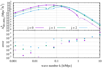
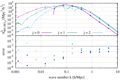
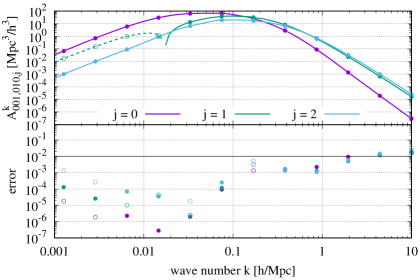
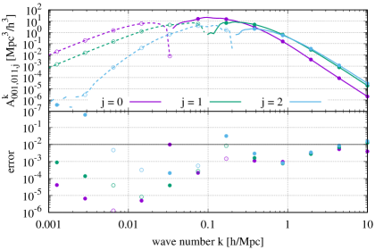
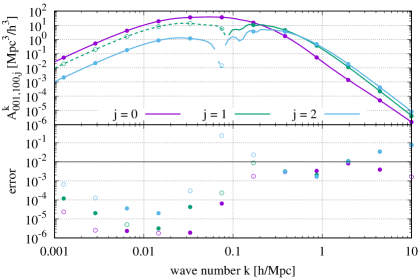
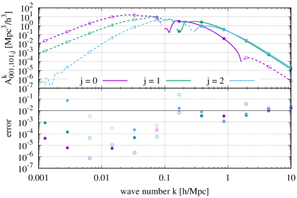
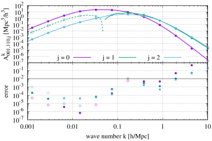
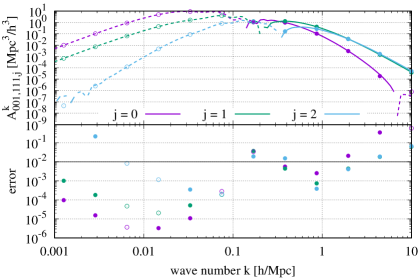
Figure 1: Mode-coupling integrals $A_{\alpha,001,bef,j}^{k}$ of Eqs. (3.27-3.29) computed using the FFT techniques of Sections 4-5 (lines) compared against direct numerical integration of Eq. (2.23) (points). Dashed lines and open points denote negative values. Within each plot, the upper panel shows $A_{\alpha,001,bef,j}^{k}$ and the lower panel the fractional error in the FFT computation. The $A_{\alpha,001,bef,j}^{k}$ are plotted using $z=0$ linear power spectra and $N_{\mu,\mathrm{NL}}=3$ angular modes for a neutrino flow with $v_{\alpha}=0.00154=461$ km/s.

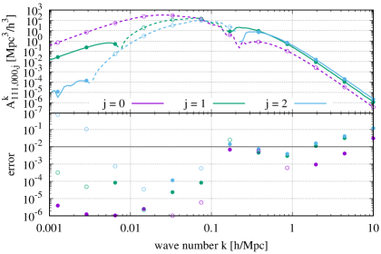
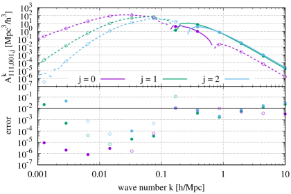
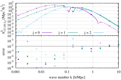
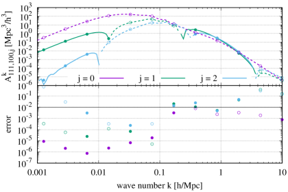
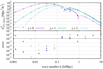
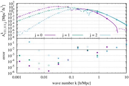
Figure 2: Similar to Fig. 1 but for $A_{\alpha,111,bef,j}^{k}$. The symmetry $A_{\alpha,111,bef,j}^{k}=A_{\alpha,111,bfe,j}^{k}$ means that there are only six unique integrals of this type.

Errors in the FFT-accelerated mode-coupling integrals are less than $1\%$ over a broad range of wave numbers, with a few important exceptions:

1. regions near a zero of a given mode-coupling integral;

2. small scales, corresponding to wave numbers $k\gtrsim 2~{}h/$Mpc;

3. large scales, corresponding to wave numbers $k\lesssim 0.005~{}h/$Mpc, particularly for $j>1$.

Fourier transforms mix numerical errors across the entire $k$ range. Each $A_{\alpha,acd,bef,j}^{k}$ has a large dynamic range, so FFT acceleration turns small relative errors around the peak of $A_{\alpha,acd,bef,j}^{k}$ into large relative errors where $A_{\alpha,acd,bef,j}^{k}$ is small. Since the power spectra for higher Legendre moments are suppressed by more factors of $kv_{\alpha}/{\mathcal{H}}$, which is small at low $k$, this translates into larger low-$k$ errors for larger $j$.

Note, however, that within a large range of wave numbers around the free-streaming scale, $k_{\mathrm{FS}}\approx 0.2~{}h/$Mpc for this model, the error in a particular FFT-accelerated $A_{\alpha,acd,bef,j}^{k}$ exceeds $1\%$ only where that integral is small, and therefore subdominant to other mode-coupling integrals. Moreover, $j=0$ mode-coupling integrals, which have the most direct impact on the monopole power spectrum, tend to be the most accurate.

Acceleration substantially improves the speed of the mode-coupling integral computation. Direct numerical integration with tolerances of $\epsilon_{\mathrm{abs}}=10^{-6}$ and $\epsilon_{\mathrm{rel}}=10^{-2}$ required $1800$ sec on a quad-core desktop computer. FFT acceleration reduced the running time to $4.6$ sec, speeding the calculation by a factor of about $400$.

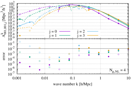
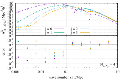
Figure 3: Similar to Fig. 1 but for $N_{\mu,\mathrm{NL}}=4$. Only the mode-coupling integrals $A_{\alpha,001,001,j}^{k}$ (left) and $A_{\alpha,111,101,j}^{k}$ (right) are shown.

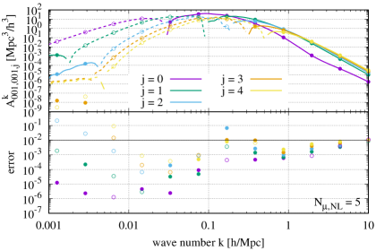
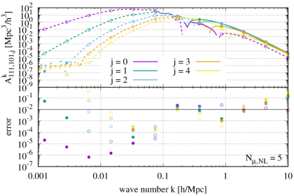
Figure 4: Similar to Fig. 1 but for $N_{\mu,\mathrm{NL}}=5$. Only the mode-coupling integrals $A_{\alpha,001,001,j}^{k}$ (left) and $A_{\alpha,111,101,j}^{k}$ (right) are shown.

Next, we consider the accuracy and computational expense of mode-coupling integrals with more angular modes $N_{\mu,\mathrm{NL}}$. We focus on two representative mode-coupling integrals: $A_{\alpha,001,001,j}^{k}$, the non-linear source for $I_{\alpha,001,001,j}^{k}$, which enhances density clustering; and $A_{\alpha,111,101,j}^{k}$, because it has the largest errors in the $0.1~{}h/{\rm Mpc}<k<1~{}h/{\rm Mpc}$ range.

Figures 3 and 4 plot these two mode-coupling integrals for $N_{\mu,\mathrm{NL}}$ of $4$ and $5$, respectively. Most encouragingly, $A_{\alpha,001,001,j}^{k}$ is accurate to $\leq 1\%$ for $k$ within an order of magnitude of the free-streaming scale $k\sim 0.2~{}h/$Mpc except for $A_{\alpha,001,001,2}^{k}$ and $A_{\alpha,001,001,3}^{k}$ near their zeros. Furthermore, increasing $N_{\mu,\mathrm{NL}}$ does not appear to worsen errors in $A_{\alpha,111,101,j}^{k}$, which for $N_{\mu,\mathrm{NL}}=5$ remain under $3\%$ over the same $k$ range.

Examination of the higher-$j$ mode-coupling integrals shows a floor $\sim 10^{-6}~{}{\rm Mpc}^{3}/h^{3}$ below which $A_{\alpha,acd,bef,j}^{k}$ becomes dominated by noise. This floor is about seven or eight orders of magnitude below the peak of each mode-coupling integral. For all $j$ shown, mode-coupling integrals become noise-dominated well below $k=0.01~{}h/$Mpc. Fortunately, neutrino non-linearities are negligible in that regime. In order to prevent this numerical noise from contaminating our calculation, we neglect non-linear corrections below some $k_{\rm low}\sim 0.01~{}h/$Mpc, following the suggestion of Ref. [85] for ordinary Time-RG.

Increasing $N_{\mu,\mathrm{NL}}$ from $3$ to $4$ and $5$ increases the computation time for the full set of mode-coupling integrals from $4.6$ sec to $23.5$ sec and $87$ sec, respectively on a four-processor desktop computer. FFT acceleration therefore provides non-linear mode-coupling integrals at a reasonable computational cost, and with $\sim 1\%$-level accuracy over a broad range of scales on either side of the free-streaming scale. In the next Section we include these mode-coupling integrals in a complete non-linear perturbation theory for the massive neutrinos.

6 FlowsForTheMasses and non-linear enhancement of neutrino power

6.1 Procedure, convergence, and computational cost

At last we assemble the multi-fluid linear theory of Sec. 2.1 and Refs. [72, 73, 45], the non-linear equations of motion from Sec. 3, and the non-linear mode-coupling integrals of Secs. 4 and 5, into a complete non-linear perturbative code using multiple flows to represent the massive neutrinos, which we call FlowsForTheMasses.

Throughout this Section, unless otherwise identified, we assume a $\nu\Lambda$CDM cosmology with the following parameters:

$$h = 0.6766;\quad n_{\mathrm{s}}=0.9665;\quad A_{\mathrm{s}}=2.135\times 10^{-9};$$

$$\Omega_{\mathrm{m},0}h^{2} = 0.14175;\quad\Omega_{\mathrm{b},0}h^{2}=0.02242;\quad\Omega_{\nu,0}h^{2}=0.005.$$ (6.1)

This neutrino density is near the upper limit allowed by recent analyses such as Refs. [7, 9] provided that the dark energy equation of state and its first derivative are also allowed to vary. We treat the three neutrino species as degenerate, corresponding to a single neutrino mass $m_{\nu}=0.155$ eV and a free-streaming scale $k_{\mathrm{FS}}=0.13(1+z)^{-1/2}~{}h/$Mpc [86, 87].

Section 5.4 noted a numerical noise arising at $k\lesssim 0.01~{}h/$Mpc for mode-coupling integrals $A_{\alpha,acd,bef,j}^{k}$ with $j\gtrsim 3$. Since non-linear corrections to neutrino clustering are negligible in that region, FlowsForTheMasses smoothly turns off low-$k$ non-linear corrections by multiplying each mode-coupling integral in Eq. (3.18) by a low-$k$ suppression factor:

$$A_{\alpha,acd,bef,j}^{k}\longrightarrow A_{\alpha,acd,bef,j}^{k}\times\frac{2}{[1+e^{(k_{\rm low}/k)^{4}}]}\quad\mathrm{with}~{}k_{\rm low}=0.01~{}h/\mathrm{Mpc.}$$ (6.2)

$N_{\mu,\mathrm{NL}}$	$1$	$2$	$3$	$4$	$5$	$6$	$7$	$8$	$9$
Cost [sec]	$0.079$	$0.58$	$4.6$	$23.5$	$87$	$250$	$630$	$1380$	$2780$
$k_{\mathrm{stab}}$ [$h/$Mpc]	$\geq 10$	$\geq 10$	$\geq 10$	$4.8$	$4.4$	$4.4$	$3.7$	$3.7$	$0$

Table 1: Computational cost and stability region of FlowsForTheMasses integration vs. number of angular modes $N_{\mu,\mathrm{NL}}$ used in non-linear mode-coupling integrals. The cost is the time required to run a full set of mode-coupling integrals $A_{\alpha,acd,bef,j}^{k}$ for a single fluid at a single time step over $N_{k}=128$ logarithmically-spaced wave numbers $k$ on a standard four-processor desktop machine. The numerical stability threshold $k_{\mathrm{stab}}$ is the maximum wave number to which the equations of motion, Eqs. (3.10-3.13), can be integrated for the model of Eq. (6.1), as discussed in Sec. 6.2. For $N_{\mu,\mathrm{NL}}=9$, instabilities prevented integration of the equations of motion below $z=0.7$.

Table 1 lists the computational cost of a mode-coupling integral computation for a range of $N_{\mu,\mathrm{NL}}$. Even including the $400$-fold speed improvement through FFT acceleration techniques in FlowsForTheMasses, neutrino mode-coupling integrals for large $N_{\mu,\mathrm{NL}}$ remain computationally expensive, due to the ${\mathcal{O}}(N_{\mu,\mathrm{NL}}^{6})$ scaling of the $P^{(2,2)}$-type integrals identified in Sec. 4.3. The running times in the table, for a single fluid $\alpha$ at a single time step, assuming $N_{k}=128$ wave numbers, is approximated by ($0.005N_{\mu,\mathrm{NL}}^{6}+0.07N_{\mu,\mathrm{NL}}^{2}$) seconds.

We mitigate this computational cost in two ways. Firstly, we do not include non-linear corrections for a given flow $\alpha$ until its maximum dimensionless density monopole power $\Delta_{\alpha 000}^{2}(k)=k^{3}P_{\alpha 000}^{k}/(2\pi^{2})$ exceeds a predetermined threshold of $\Delta^{2}_{\mathrm{thresh}}=10^{-4}$. Following Ref. [82], we initialize $I_{\alpha,acd,bef,j}^{k}$ to $2A_{\alpha,acd,bef,j}^{k}$ once this threshold is reached.

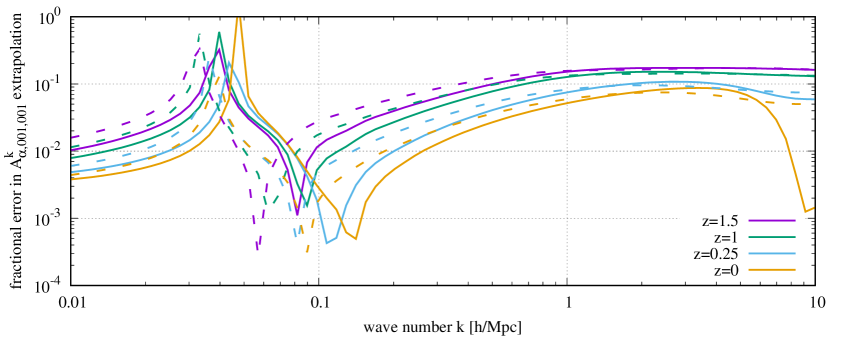
Figure 5: Maximum extrapolation error in mode-coupling integrals $A_{\alpha,001,001,0}^{k}$ for $\alpha=0$ (solid) and $\alpha=1$ (dashed). We fix $N_{\mu,\mathrm{NL}}=3$.

Secondly, even when this threshold is crossed, we restrict computation of neutrino mode-coupling integrals to the $N_{a}=50$ scale factors $a_{n}=0.02n$ for $1\leq n\leq N_{a}$. Between these computation times, we approximate each $A_{\alpha,acd,bef,j}^{k}$ as scaling like the clustering-limit monopole power spectra in its integrand, that is, as $(\delta_{\alpha,0}^{0})^{3-b-e-f}(\theta_{\alpha,0}^{0})^{1+b+e+f}$. The error associated with this approximation is greatest just before one of the $a_{n}$, when mode-coupling integrals from step $a_{n-1}$ are extrapolated all the way to $a_{n}$.

Figure 5 quantifies the maximum error in $A_{\alpha,001,001,0}^{k}$ resulting from this extrapolation for the case of $N_{\tau}=10$ flows. Around $k_{\mathrm{FS}}$ the error is no more than $4\%$ for $z\leq 1.5$. At $z=0$, where non-linear corrections are most significant, the error is $<1\%$ around $k=k_{\mathrm{FS}}$ and no more than $6\%$ at any $k_{\mathrm{FS}}\leq k\leq 1~{}h/$Mpc. Aside from $k\approx 0.04~{}h/$Mpc, where the mode-coupling integrals pass through zero, the maximum error resulting from this extrapolation for $z\leq 0.25$ is $\lesssim 10\%$. This decrease in error with rising scale factor is due to our choice of $a_{n}$, since the fractional increase $(a_{n+1}-a_{n})/a_{n}$ is lower at larger scale factors.

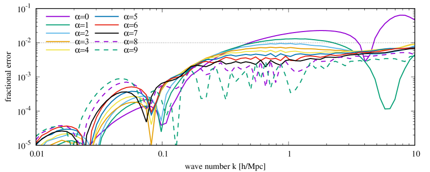
Figure 6: Density monopole errors at $z=0$ associated with neglecting neutrino non-linearity below the threshold $\Delta^{2}_{\mathrm{thresh}}=10^{-4}$ and computing mode-coupling integrals only at $a_{n}=0.02n$.

Combined errors due to both of these approximations are quantified by reducing both the $\Delta^{2}$ threshold and the spacing between mode-coupling recomputations. Figure 6 compares our default calculation above to one whose threshold is ten times smaller, $\Delta^{2}_{\mathrm{thresh}}=10^{-5}$, and whose mode-coupling integrals are computed four times more frequently, $a_{n}=0.005n$. In the $k\leq 1~{}h/$Mpc range, the resulting error is about $2\%$ for $\alpha=0$. Across the entire $k$ range, errors are under $1.5\%$ for $\alpha=1$, and under a percent for all higher-$\alpha$ flows. Thus we regard these two approximations as well-founded. Henceforth we use $\Delta^{2}_{\mathrm{thresh}}=10^{-4}$ and $a_{n}=0.02n$ in all of our FlowsForTheMasses computations.

Also listed in Table 1 is the maximum wave number $k_{\mathrm{kstab}}$ to which our integration of the equations of motion is stable. In practice we integrate Eqs. (3.10-3.13) using a $5$th-order Runge-Kutta method with adaptive step size control, as implemented in the GNU Scientific Library (GSL) of Ref. [88]. We begin with $k_{\mathrm{stab}}$ set to the maximum wave number considered, $10~{}h/$Mpc. Each time that the GSL integrator is unable to progress, we reduce $k_{\mathrm{stab}}$ by one step, or a factor of $\exp({\mathcal{D}}_{k})$, and resume integration.

Evidently, FlowsForTheMasses is numerically stable for a broad range of wave numbers reaching $\approx 30$ times the free-streaming scale. For $N_{\mu,\mathrm{NL}}\geq 6$, we have also raised $k_{\mathrm{low}}$ in Eq. (6.2) to $0.05~{}h/$Mpc to mitigate low-$k$ noise. For $N_{\mu,\mathrm{NL}}=9$, the highest value considered here, we were unable to integrate the equations of motion all the way to $z=0$. Integration reached $z=0.7$ with a stability threshold of $0.5~{}h/$Mpc before failing. Henceforth we only consider $N_{\mu,\mathrm{NL}}\leq 8$. We also caution that, for a large number $N_{\tau}$ of flows, the slowest will be much more non-linear than those considered here, hence will reach our non-linear threshold $\Delta^{2}_{\mathrm{thresh}}=10^{-4}$ sooner, leaving more time for numerical instabilities to develop.

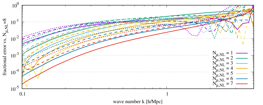
Figure 7: Convergence of the $z=0$ density monopole perturbation $\delta_{\alpha 0}^{k}$ for $\alpha=0$ (solid lines), $\alpha=1$ (dashed), and $\alpha=2$ (dotted), assuming $N_{\tau}=10$ flows in total. The error in each perturbation is quantified by comparison to the $N_{\mu,\mathrm{NL}}=8$ case.

Finally, we discuss convergence of the code with increasing $N_{\mu,\mathrm{NL}}$. Again considering $N_{\tau}=10$ flows, Fig. 7 quantifies the error in each $\delta_{\alpha 0}^{k}$ for a given $N_{\mu,\mathrm{NL}}$ by comparison to $N_{\mu,\mathrm{NL}}=8$. At the free-streaming scale, perturbation theory is accurate at the percent level for $N_{\mu,\mathrm{NL}}\geq 3$. In the range $k\lesssim 2~{}h/$Mpc, perturbation theory is converging, in the sense that its errors continue declining as $N_{\mu,\mathrm{NL}}$ is increased. For $k\leq 1~{}h/$Mpc, the $\alpha=0$ density monopoles are $8\%$ accurate for $N_{\mu,\mathrm{NL}}=5$, $4\%$ for $N_{\mu,\mathrm{NL}}=6$, and $2.5\%$ for $N_{\mu,\mathrm{NL}}=7$. Thus FlowsForTheMasses is convergent and accurate for computing the neutrino power spectrum all the way up to $k=1~{}h/$Mpc. In the remainder of this Section, we will: (i) couple neutrinos to a Time-RG CDM+baryon fluid, illustrating the high-$z$ and qualitative low-$z$ behavior of their non-linear corrections; (ii) couple neutrinos to a more accurate calculation of CDM+baryon clustering emulated from N-body simulations, providing neutrino power computations that are reliable even at low redshifts; (iii) describe a set of simulations carried out by a companion article, Ref. [79]; (iv) demonstrate the accuracy of FlowsForTheMasses using these simulations; and (v) explore the dependency of non-linearity upon neutrino mass.

6.2 FlowsForTheMasses with Time-RG perturbations for CDM, baryons

As a first application of FlowsForTheMasses, we pair it with a Time-RG perturbative evolution of the CDM+baryon fluid. We begin by considering the neutrino power spectra themselves. Working in the cosmological model of Eq. (6.1), we discretize the massive neutrino population into $N_{\tau}=10$ velocity bins, with $0\leq\alpha\leq 9$, and $N_{\mu}=10$ angular modes, with $0\leq\ell\leq 9$. Velocities corresponding to these bins are listed in Table 2. Figure 8 shows our monopole ($\ell=0$) power spectra for several values of $N_{\mu,\mathrm{NL}}$, the number of angular modes used to compute the mode-coupling integrals. Note that $N_{\mu,\mathrm{NL}}$ of one is equivalent to the ordinary Time-RG of Ref. [68] with a modified linear evolution matrix $\Xi_{\alpha ab0}^{k}$, while increasing $N_{\mu,\mathrm{NL}}$ includes more of the corrections developed in this work.

$\alpha$	$0$	$1$	$2$	$3$	$4$	$5$	$6$	$7$	$8$	$9$
$v_{\alpha}/c$	$0.00101$	$0.0016$	$0.00204$	$0.00245$	$0.00286$	$0.0033$	$0.0038$	$0.00442$	$0.00528$	$0.00697$

Table 2: Velocities $v_{\alpha}$ at $z=0$ for $N_{\tau}=10$ flows in the cosmological model of Eq. (6.1).

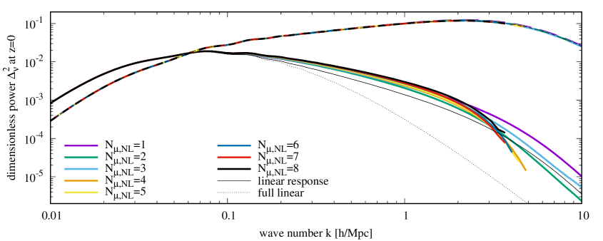
Figure 8: Dimensionless $z=0$ neutrino monopole power spectra $\Delta^{2}_{aa0}(k)=\frac{k^{3}}{2\pi^{2}}P_{aa0}(k)$ for a range of $N_{\mu,\mathrm{NL}}$, for the model of Eq. (6.1). Solid lines show the $\delta$ power spectrum ($a=0$) and dashed lines the $\theta$ power spectrum ($a=1$). The multi-fluid linear response of Ref. [45] is shown for comparison.

Velocity power spectra are large at small scales due to free streaming. Non-linear corrections to them are negligibly small, a few percent at most, for all $N_{\mu,\mathrm{NL}}$. Evidently, linear response accurately captures the behavior of the neutrino velocity dispersion power spectrum down to very small scales, $k=10~{}h/$Mpc. Thus the remainder of this Section will focus on the power spectra of density perturbations.

Regarding the density power spectra in Fig. 8, all of the non-linear power spectra $N_{\mu,\mathrm{NL}}\geq 1$ in the region $k\sim 1~{}h/$Mpc are $\sim 2$ times larger than the linear response power spectrum. At somewhat smaller scales, $k\gtrsim 2~{}h/{\rm Mpc}$, $N_{\mu,\mathrm{NL}}$ of $1$ overpredicts clustering relative to larger values, while $N_{\mu,\mathrm{NL}}$ of $2$ underpredicts it. Evidently from Eq. (3.11), free-streaming suppression of the monopole $\delta_{\alpha 0}^{k}$ is proportional to the dipole $\delta_{\alpha 1}^{k}$. By including a non-linear enhancement to this dipole, $N_{\mu,\mathrm{NL}}=2$ indirectly suppresses the monopole. In turn, $N_{\mu,\mathrm{NL}}=3$ includes an enhancement of the quadrupole $\delta_{\alpha 2}^{k}$, which indirectly enhances the monopole by suppressing the dipole. Thus we recommend at least $N_{\mu,\mathrm{NL}}=3$.

At still smaller scales, $2~{}h/{\rm Mpc}<k\lesssim 4~{}h/{\rm Mpc}$, power spectra using the higher $N_{\mu,\mathrm{NL}}$ drop sharply, falling below the linear response power. For $N_{\mu,\mathrm{NL}}\geq 4$, we encounter the numerical instabilities listed in Table 1. Integration of the equations of motion fails to converge for $k\gtrsim 4~{}h/$Mpc, suggesting that this drop below $4~{}h/$Mpc is the result of the same numerical instability. References [82, 85, 45] have noted and mitigated small-scale numerical instabilities in ordinary Time-RG for a cold fluid. These are due in part to the scalarized equations of motion for $\delta$ and $\theta$ neglecting small-scale velocity vorticity. Our perturbation theory appears to exacerbate these small-scale instabilities at high $N_{\mu,\mathrm{NL}}$.

Neutrino clustering is dominated at very large scales, $k\ll k_{\mathrm{FS}}$, by fully linear growth; at intermediate scales, $k\sim k_{\mathrm{FS}}$, by linear response to non-linear CDM+baryon growth; and at small scales, $k\gg k_{\mathrm{FS}}$, by non-linear growth. We define the non-linear enhancement

$$E_{\alpha a\ell}^{k}:=P_{\alpha aa\ell}^{k}/P_{\alpha aa\ell}^{\mathrm{[MFLR]}k}-1$$ (6.3)

where $P_{\alpha aa\ell}^{\mathrm{[MFLR]}k}$ is the power spectrum computed using the Multi-Fluid Linear Response (MFLR) method of Ref. [45]. We will devote the remainder of this Section to computing $E_{\alpha a\ell}^{k}$ and comparing it against the enhancement seen in N-body simulations including massive neutrino particles. We begin with the calculation described above, with FlowsForTheMasses coupled to CDM and baryons evolved using Time-RG perturbation theory.

Here we study the enhancement in the region $k\leq 1~{}h/$Mpc, well below the unphysical power suppression at $k\sim 4~{}h/$Mpc. We begin with the total monopole enhancement

$$E_{\Sigma\alpha,a,0}^{k}:=\left(\Sigma_{\alpha}\psi_{\alpha a0}^{k}/N_{\tau}\right)^{2}/\left(\Sigma_{\alpha}\psi_{\alpha a0}^{[\mathrm{MFLR}]k}/N_{\tau}\right)^{2}-1.$$ (6.4)

Figure 9 shows the total enhancements of the density and velocity power spectra. Density enhancement rises from a few percent at the free-streaming scale to $\approx 100\%$ at $k=1~{}h/$Mpc. The enhancement for $N_{\mu,\mathrm{NL}}=7$ is within $5\%$ of that for $N_{\mu,\mathrm{NL}}=8$ up to $k=0.4~{}h/$Mpc; within $10\%$ up to $k=0.7~{}h/$Mpc, or about five times $k_{\mathrm{FS}}$; and within $14\%$ up to $k=1~{}h/$Mpc. Velocity enhancement is no more than a few percent for any $N_{\mu,\mathrm{NL}}$.

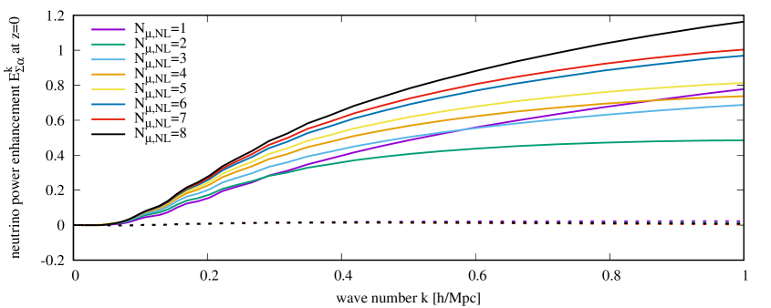
Figure 9: Monopole non-linear enhancement of Eq. (6.4) at $z=0$ for the model of Eq. (6.1). Solid lines show the density ($a=0$) enhancement and dashed lines the velocity ($a=1$) enhancement.

Considering the neutrino power, rather than the enhancement, $N_{\mu,\mathrm{NL}}=3$ agrees with $N_{\mu,\mathrm{NL}}=8$ to $10\%$ up to $k=0.3~{}h/$Mpc and to $20\%$ up to $k=0.8~{}h/$Mpc. Meanwhile, $N_{\mu,\mathrm{NL}}$ of $4$ and $5$ are accurate to $10\%$ up to $k$ of $0.4~{}h/$Mpc and $0.5~{}h/$Mpc, respectively, and to $<20\%$ across the entire range $k\leq 1~{}h/$Mpc, while $N_{\mu,\mathrm{NL}}$ of $6$ and $7$ are accurate to $5\%$ up to $k$ of $0.4~{}h/$Mpc and $0.7~{}h/$Mpc, respectively, and to $<10\%$ for $k\leq 1~{}h/$Mpc.

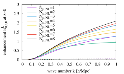
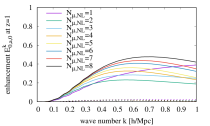
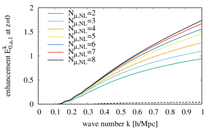
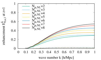
Figure 10: Neutrino enhancement $E_{\alpha a\ell}^{k}$ for $\alpha=0$; $\ell$ of $0$ (top row) and $1$ (bottom row); at $z=0$ (left column) and $z=1$ (right column) for a range of $N_{\mu,\mathrm{NL}}$. Enhancements to $P_{\alpha 00\ell}^{k}$ are shown as solid lines and those to $P_{\alpha 11\ell}^{k}$ as dotted lines.

Next, we consider the power enhancement for the individual $\alpha=0$ flow using Eq. (6.3). Figure 10 shows the density and velocity enhancements for $\ell=0$ and $1$, each at redshifts $0$ and $1$. Dipole enhancements are not shown for $N_{\mu,\mathrm{NL}}=1$, which only applies non-linear corrections to the monopole. Since $\alpha=0$ corresponds to the slowest-moving, hence the most strongly-clustering, of the neutrino flows, its $z=0$ density enhancement is approximately twice the average value of Fig. 9. For $N_{\mu,\mathrm{NL}}=8$ and $k=1~{}h/$Mpc, the enhancement is greater than two, implying that non-linear corrections more than triple the $\alpha=0$ linear response power spectrum at this scale. Even at $z=1$, non-linear corrections represent an $\approx 50\%$ enhancement to the linear response power. The dipole density power enhancements at both redshifts are comparable in magnitude to the monopole enhancements.

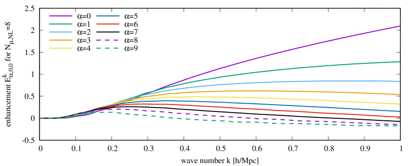
Figure 11: Neutrino density monopole enhancement for all $\alpha$, at $z=0$, with $N_{\mu,\mathrm{NL}}=8$ fixed.

Figure 11 fixes $N_{\mu,\mathrm{NL}}=8$ and displays the density monopole enhancements for all $0\leq\alpha<N_{\tau}=10$. The enhancement for $\alpha=1$ plateaus at about two-thirds the value of $E_{000}^{1~{}h/{\rm Mpc}}$, while $E_{200}^{k}$ peaks at less than half of this value. The total density monopole enhancement for $5\leq\alpha\leq 9$, or Eq. (6.4) but with both summations limited to $5\leq\alpha\leq 9$, peaks at $28\%$. However, these flows cluster so weakly that this enhancement always represents less than $1\%$ of the total power. Thus a high-accuracy calculation of the neutrino power spectrum could neglect non-linearity in these flows altogether. Similarly, neglecting the flows $3\leq\alpha\leq 9$ would only introduce a $3.5\%$ error into a power spectrum calculation.

In summary, we have shown that our self-contained non-linear perturbative calculation for massive neutrinos and the CDM+baryon fluid has converged at the ${\mathcal{O}}(10\%)$ level across the range $k\lesssim 1~{}h/$Mpc. Non-linear growth increases the density power in the model of Eq. (6.1) by a factor of more than $2$ at $k=1~{}h/$Mpc, meaning that it cannot be neglected in any computation of the neutrino power spectrum.

6.3 FlowsForTheMasses with N-body CDM+baryon source

One source of error in the previous Section is its use of Time-RG perturbation theory for the CDM+baryon fluid, whose clustering is highly non-linear at small scales and late times. References [81, 7] show that Time-RG is roughly accurate down to $z\approx 1$ but breaks down for $z\lesssim 0.5$. Since the CDM+baryon fluid makes up the significant majority of the total matter, and hence the gravitational source for neutrino clustering, its Time-RG perturbation theory errors impact our $E_{\alpha aj}^{k}$ calculations.

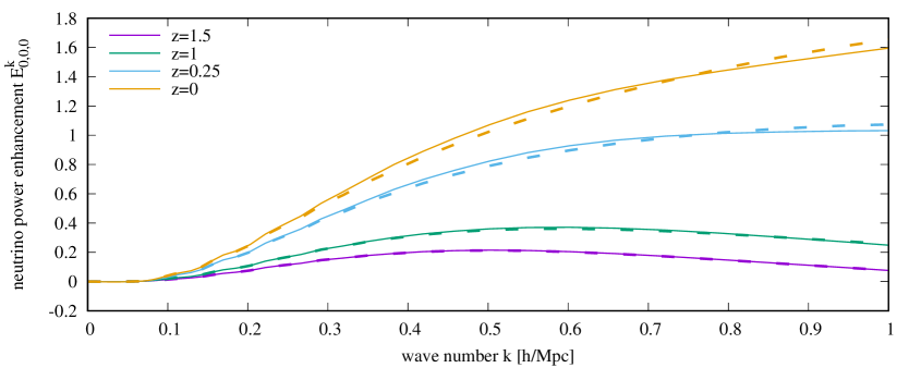
Figure 12: Neutrino density monopole enhancement for $\alpha=0$, for a range of $z$, with $N_{\mu,\mathrm{NL}}=5$ fixed. Solid lines show the neutrino $E_{\alpha,0,0}^{k}$ using the emulated CDM+baryon power spectrum of Ref. [89], while dashed lines use Time-RG for the CDM and baryons as in Sec. 6.2.

In order to quantify this error, we include in FlowsForTheMasses the CDM+baryon power spectrum computed by the Mira-Titan IV emulator of Ref. [89]. This is calibrated against a suite of N-body simulations which account for neutrinos purely linearly, an approximation whose impact on the CDM+baryon power was limited to $\lesssim 0.1\%$ in Ref. [45]. Specifically, for $z\leq 2$ we replace the CDM+baryon density $\delta_{\mathrm{cb}}$ in $\Phi$ of Eq. (2.7) by the square root of the corresponding emulator power. Above $z=2$, the upper limit of the emulated power spectrum, we return to Time-RG for the CDM and baryons.

Neutrino power spectra resulting from this emulated CDM+baryon source are somewhat smaller than those in Fig. 8, for example about $10\%$ smaller at $z=0$ and $k=1~{}h/$Mpc. Importantly, the breakdown in FlowsForTheMasses around $k=4~{}h/$Mpc for $N_{\mu,\mathrm{NL}}\geq 4$ persists. Thus this instability affects neutrino perturbation theory directly, rather than through a Time-RG error in the CDM+baryon sector.

Figure 12 compares the $\alpha=0$ neutrino density monopole enhancements for emulated and perturbative CDM+baryon sources. Differences are small at high redshifts, amounting to just $0.9\%$ of the linear response power spectrum at $z=1$ and $k=1~{}h/$Mpc. This difference rises to $6\%$ at $z=0$. Thus Time-RG perturbation theory for the CDM+baryon fluid accurately quantifies the neutrino non-linear enhancement down to $z=1$, and is sufficiently accurate for estimates and convergence tests of FlowsForTheMasses even at lower redshifts.

6.4 Hybrid N-body neutrino simulations

Hybrid N-body simulations carried out in our companion paper, Ref. [79], and run on the Katana cluster [90], also divided the neutrino population into $N_{\tau}$ flows. Each of these was evolved using either the multi-fluid linear response perturbation theory of Ref. [45] or through a realization as dynamical particles whose masses, positions, and velocities quantified the density and velocity perturbations of that flow. This hybrid simulation procedure was implemented by modifying the Gadget-4 code of Ref. [91] based upon the earlier modifications of Ref. [45]. In practice our simulations use $N_{\tau}=20$ flows but realize pairs of flows as particles, making the first pair similar to our $\alpha=0$ flow above, the next pair to $\alpha=1$, etc.

Reference [79] showed that non-linear clustering of neutrinos for the model of Eq. (6.1) represented only a $0.2\%$ correction to the total matter power spectrum, which sources the gravitational potential. Thus we quantify the non-linear enhancement $E_{\alpha a\ell}^{k}$ of a single flow $\alpha$ by realizing only that flow as simulation particles, while all others are tracked using multi-fluid linear response, with the resulting error well below a percent.

Each of our hybrid N-body simulations uses $512^{3}$ particles for the CDM+baryon fluid and an additional $512^{3}$ for the neutrino flow being realized as particles. All particles were initialized at $z=99$ using the Zel’dovich approximation for initial velocities, which Ref. [92] showed to be $\approx 2\%$ accurate for $k\leq 1~{}h/$Mpc, and we included an additional randomly-directed comoving velocity of magnitude $v_{\alpha}$ for the neutrino particles. Weak neutrino clustering at small scales makes the neutrino power spectrum especially prone to contamination by shot noise. We mitigated this through the use of small simulation volumes, cubic boxes with edge lengths $L$ of either $256$ Mpc$/h$ or $128$ Mpc/h, and for which we assumed periodic boundary conditions. The larger-box simulation used a force-softening length of $20$ kpc$/h$, while the smaller-box simulation used $10$ kpc$/h$. From each simulated power spectrum we subtracted the approximate shot noise $L^{3}/N$, though residual noise remains.

6.5 Comparison to hybrid N-body simulations

We begin with a test of FlowsForTheMasses in conjuction with Time-RG perturbation theory for the CDM+baryon fluid, as discussed in Sec. 6.2. Since the CDM and baryons cluster very non-linearly at late times, their perturbative treatment is unreliable for $z\lesssim 0.5$. Thus in Fig. 13 we compare the N-body and perturbative enhancements only at $z=1$. N-body enhancements are smoothed using a centered $20$-point moving average.

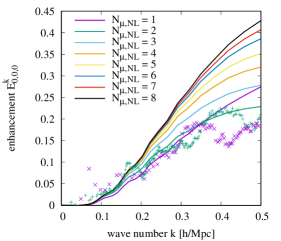
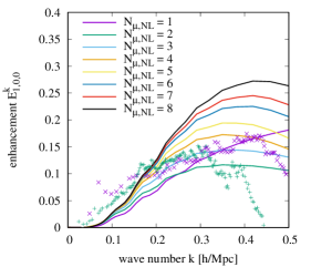
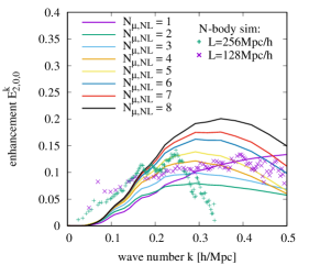
Figure 13: Neutrino density monopole enhancement for $\alpha$ of $0$, $1$, and $2$ at redshift $z=1$. Shown are the non-linear perturbative calculations (thick lines) and hybrid N-body computations (points).

Neutrino clustering at $z=1$ is weak and its power spectrum is dominated by linear response. Thus N-body measurements of the enhancement are quite noisy. Figure 13 shows that the N-body enhancement drops below all of the perturbative calculations at $k=0.5~{}h/$Mpc for $\alpha=0$ and even falls below zero for larger $\alpha$. Focusing on the region $k\lesssim 2k_{\mathrm{FS}}\approx 0.25~{}h/$Mpc, we see close agreement between N-body and perturbative $E_{\alpha 00}^{k}$. Agreement is closest for $N_{\mu,\mathrm{NL}}\geq 3$, though noise in the N-body enhancements makes a more detailed comparison difficult. At larger scales, $k\lesssim k_{\mathrm{FS}}$, perturbation theory underpredicts power by a few percent, possibly due to the free-streaming closure approximation of Sec. 3.2.

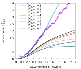
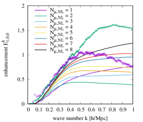
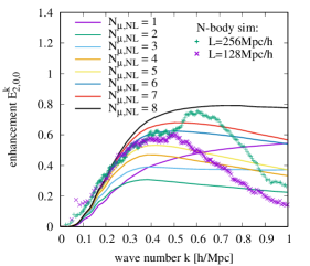
Figure 14: Neutrino density monopole enhancement for $\alpha$ of $0$, $1$, and $2$ at redshift $z=0$. CDM+baryon power below a redshift of $2$ was computed using the emulator of Ref. [89]. Shown are the non-linear perturbative calculations (thick lines) as well as hybrid N-body computations (points).

Testing FlowsForTheMasses at $z=0$ requires a more accurate calculation of the CDM+baryon power such as that emulated in Ref. [89], as discussed in Sec. 6.3. Figure 14 compares our perturbation theory sourced by this emulated power to the hybrid simulation for $\alpha$ of $0$, $1$, and $2$ at $z=0$. The N-body enhancements are substantially less noisy than those at $z=1$. Since neutrinos cluster more strongly at late times, particularly on small scales, residual shot noise represents a smaller error at $z=0$.

Evidently perturbation theory for $\alpha=2$ agrees closely with the N-body enhancement in Fig. 14 (right). Agreement is best for $N_{\mu,\mathrm{NL}}\geq 3$ in the region $k\leq 2k_{\mathrm{FS}}\approx 0.25~{}h/$Mpc and for $N_{\mu,\mathrm{NL}}\geq 5$ in the region $k\leq 4k_{\mathrm{FS}}\approx 0.5~{}h/$Mpc. Beyond this $k$ range, the N-body enhancement becomes noisy and its agreement with perturbation theory difficult to assess. Moreover, at $k\gtrsim 0.5~{}h/$Mpc we see disagreements between our own simulations, with the $L=256$ Mpc$/h$ box likely suffering from larger residual shot noise, but the $L=128$ Mpc$/h$ box systematically underpredicting power due to neglecting perturbations larger than the box size. Nevertheless, we may conclude that FlowsForTheMasses accurately captures the non-linear enhancement for $\alpha\geq 2$, or $80\%$ of the total neutrino population for the model of Eq. (6.1), down to $z=0$, over the range $k\lesssim 4k_{\mathrm{FS}}$.

Perturbation theory is still impressive for the second-slowest flow, $\alpha=1$. It agrees reasonably well with simulations up to $k/k_{\mathrm{FS}}$ of $1.5-2$. Even up to $k=1~{}h/$Mpc, the perturbation theory error in $E_{1,0,0}^{k}$ is limited to about $0.5$, representing an $\approx 25\%$ in the density monopole power spectrum for that flow. Since $\alpha=1$ itself represents $10\%$ of the neutrino population, perturbation theory is useful for this flow in an accurate calculation of the total neutrino power spectrum.

N-body power for the slowest flow, shown in Fig. 14 (left), is far in excess of any of the perturbative calculations for $k\gtrsim 3k_{\mathrm{FS}}$. Perturbation theory has clearly converged in this region; errors in $\delta_{00}^{3k_{\mathrm{FS}}}$ for $N_{\mu,\mathrm{NL}}$ of $1-7$, relative to $N_{\mu,\mathrm{NL}}=8$, are respectively $8\%$, $7\%$, $4.5\%$, $2.6\%$, $1.6\%$, $0.79\%$, and $0.34\%$. Thus we must conclude that perturbation theory itself is inaccurate for $\alpha=0$ at small scales. This accords with our intuition that perturbation theory will break down as $E_{\alpha a\ell}^{k}$ approaches unity for a given $\alpha$. A percent-level-accurate computation of the small-scale neutrino power spectrum must use a particle treatment at least for flow $\alpha=0$ in the range $z<1$.

Finally, we consider the accuracy of the FlowsForTheMasses computation of the total neutrino power spectrum with an emulated CDM+baryon power. Reference [45] demonstrated that $N_{\tau}=50$ and $N_{\mu}=20$ provides $3\%$ accuracy in the linear perturbations up to $k=1~{}h/$Mpc, so we adopt those values here. We note a caveat for large $N_{\mu}$ such as $20$. Mode-coupling integrals integrate over the product of two power spectra. Thus truncating Eq. (2.14) for power spectra used in mode-couplings at $\ell=N_{\mu,\mathrm{NL}}-1$ allows the $A_{\alpha,acd,bef}^{\vec{k}}$ themselves to depend upon $\mathcal{P}_{j}(\mu_{\alpha})^{2}$ for $j$ as high as $2N_{\mu,\mathrm{NL}}-2$. Our procedure necessarily neglects $A_{\alpha,acd,bef,j}^{k}$ for which $j\geq N_{\mu}$, so raising $N_{\mu}$ to $20$ includes more high-$j$ mode-coupling integrals, making the computation more vulnerable to low-$k$ noise. Consequently, we raise $k_{\mathrm{low}}$ in Eq. (6.2) to $0.02(1+j)~{}h/$Mpc for $N_{\mu,\mathrm{NL}}=7$ and $0.01(1+j^{2})~{}h/$Mpc for $N_{\mu,\mathrm{NL}}=8$. For $N_{\mu,\mathrm{NL}}=8$, we further reduce $N_{k}$ to $64$ and $k_{\mathrm{max}}$ to $1~{}h/$Mpc in order to reduce numerical instability and computational expense. Total running times using $32$ CPUs on the Katana Cluster [90] are $27$ hours for $N_{\mu,\mathrm{NL}}=6$ and $N_{k}=128$; $66$ hours for $N_{\mu,\mathrm{NL}}=7$ and $N_{k}=128$; and $75$ hours for $N_{\mu,\mathrm{NL}}=8$ and $N_{k}=64$.

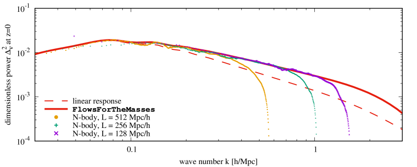
Figure 15: Dimensionless neutrino density monopole power $\Delta^{2}_{\nu}(k)$ for the model of Eq. (6.1) at redshift $z=0$. The solid line shows FlowsForTheMasses with $N_{\tau}=50$ flows, $N_{\mu}=20$ angular modes, and $N_{\mu,\mathrm{NL}}=7$; the dashed line shows multi-fluid linear response with the same $N_{\tau}$ and $N_{\mu}$; and points show the N-body power spectra with shot noise subtracted.

Figure 15 compares the resulting total neutrino power spectrum for the model of Eq. (6.1) to our hybrid N-body simulation. The N-body power realizes the slowest half of the neutrino population as particles while following the rest using multi-fluid linear response, an approximation shown in Sec. 6.2 to be accurate to within $1\%$. Agreement between FlowsForTheMasses and the N-body power is evident over a large range of wave numbers up to $k=1~{}h/$Mpc, even as both rise to more than twice the linear response power.

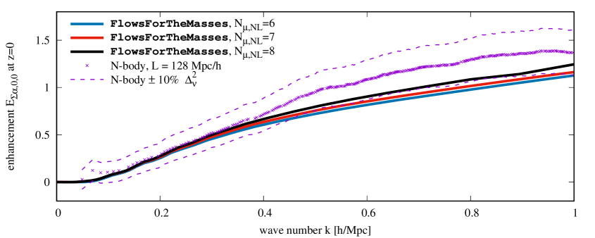
Figure 16: Neutrino density monopole enhancement $E_{\Sigma\alpha,0,0}^{k}$ for the model of Eq. (6.1) at redshift $z=0$, using FlowsForTheMasses with $N_{\tau}=50$ flows and $N_{\mu}=20$ angular modes. N-body points are smoothed using a $100$-point centered moving average.

Shown in Fig. 16 is the corresponding neutrino enhancement $E_{\Sigma\alpha,0,0}^{k}$. Up to simulation noise, the enhancements agree to $\approx 0.1$ at low $k$ and $\approx 0.2$ for $k\gtrsim 0.5~{}h/$Mpc, where $E_{\Sigma\alpha,0,0}^{k}\approx 1$. This corresponds to an agreement of $<10\%$ in the neutrino power spectra, which is impressive considering that perturbation theory was used for all neutrino flows, even the slowest. We have therefore confirmed that FlowsForTheMasses alone can predict the neutrino power spectrum to an accuracy of $10\%$ all the way up to $k=1~{}h/$Mpc for $\Omega_{\nu,0}h^{2}$ up to $0.005$, corresponding to $\sum m_{\nu}=0.47$ eV. This includes nearly the entire $95\%$CL range of Ref. [7], which allowed for substantial variations in the dark energy equation of state.

6.6 Variation of neutrino fraction

Now that we have confirmed the accuracy of a purely perturbative calculation of the non-linear neutrino power spectrum using FlowsForTheMasses, we consider the impact of varying the neutrino fraction $\Omega_{\nu,0}h^{2}$. We do so while keeping constant all other model parameters in Eq. (6.1). Since greater $\Omega_{\nu,0}h^{2}$ implies a greater non-linear enhancement, hence greater errors in perturbation theory, restricting $\Omega_{\nu,0}h^{2}\leq 0.005$ means that the perturbative power spectrum should be accurate to $<10\%$ across this entire range.

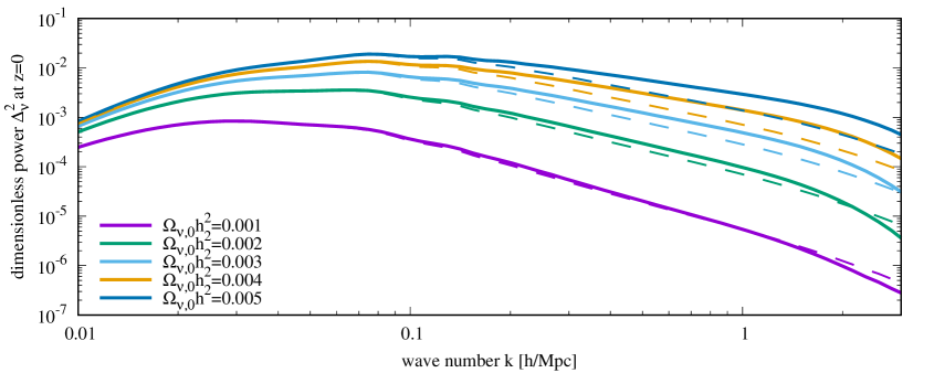
Figure 17: Dimensionless neutrino density monopole power $\Delta^{2}_{\nu}(k)$ at redshift $z=0$, using FlowsForTheMasses with $N_{\tau}=50$ flows, $N_{\mu}=20$ angular modes, and $N_{\mu,\mathrm{NL}}=6$. All cosmological parameters in Eq. (6.1) are held constant except for $\Omega_{\nu,0}h^{2}$. Thick solid lines show a FlowsForTheMasses perturbative calculation, while thin dashed lines show multi-fluid linear response.

Our results are displayed in Fig. 17. At linear scales, $k\sim 0.01~{}h/$Mpc, all power spectra are similar due to having the same normalization $A_{\rm s}$. Around the free-streaming scales, $k\sim 0.1~{}h/$Mpc for these models, significant differences in the power spectra are apparent, and non-linear enhancement has risen to $\sim 10\%$. On non-linear scales, $k\gtrsim 0.5~{}h/$Mpc, non-linear corrections are significant, doubling the power spectrum for the larger $\Omega_{\nu,0}h^{2}$. Non-linear enhancement is large enough at $k\sim 1~{}h/$Mpc that neglecting it would cause us to confuse $\Omega_{\nu,0}h^{2}$ of $0.004$ for $0.005$, a significant error in the neutrino mass fraction.

Meanwhile, for $\Omega_{\nu,0}h^{2}=0.001$, the non-linear correction peaks at $13\%$ around $k=0.2~{}h/$Mpc. Thus a power spectrum computation with an accuracy goal of $\lesssim 10\%$ may neglect a particle treatment of neutrinos up to $\Omega_{\nu,0}h^{2}=0.005$, and may neglect non-linear corrections altogether up to $\Omega_{\nu,0}h^{2}\approx 0.001$. For $\Omega_{\nu,0}h^{2}=0.002$, the non-linear correction plateaus at $38\%$ around $k=1~{}h/$Mpc. Our result is somewhat more pessimistic than that of Ref. [45], which estimated that fewer than $1\%$ of neutrinos cluster non-linearly for $\Omega_{\nu,0}h^{2}=0.002$.

Well below the free-streaming length scale, Refs. [86, 87] show that the linear response neutrino power scales as $(k_{\mathrm{FS}}/k)^{4}$ times the total matter power. Assuming all parameters except for $\Omega_{\nu,0}h^{2}$ in Eq. (6.1) are held constant, this in turn scales as $(\Omega_{\nu,0}h^{2})^{4}$. Figure 17 shows that the non-linear neutrino power spectra scale similarly. For example, at $k=1~{}h/$Mpc, the ratio of power spectra with $\Omega_{\nu,0}h^{2}$ of $0.004$ and $0.005$ is $0.47=0.83^{4}$, compared with $0.8^{4}$ predicted by the scaling relation; at $k=2~{}h/$Mpc, the ratio is $0.404=0.797^{4}$. This means that the $<10\%$ accuracy of our non-linear perturbative power spectrum is sufficient for a $<2.5\%$ accuracy in $\Omega_{\nu,0}h^{2}$, and hence the sum of neutrino masses.

7 Conclusions

We have derived, implemented, and validated the accuracy of a new non-linear cosmological perturbation theory for massive neutrinos and other hot dark matter species, which we call FlowsForTheMasses. Deriving the equations of motion, Eqs. (3.10-3.13), based upon an extension of the Time-RG perturbation theory, and Eqs. (3.18-3.26) for the bispectrum integrals, we identified the extended mode-coupling integrals $A_{\alpha,acd,bef,j}^{k}$ as the most computationally expensive components of the perturbation theory. Sections 4 and 5 constructed the computational machinery of FlowsForTheMasses by using Fast Fourier Transforms to accelerate the mode-coupling computations by more than two orders of magnitude.

In Sec. 6 we confirmed the convergence and accuracy of FlowsForTheMasses for neutrino power spectrum computations. Even for neutrino fractions as high as $\Omega_{\nu,0}h^{2}=0.005$, around the maximum allowed by the current data when the dark energy is allowed substantial freedom to vary, we find in Figs. 15 and 16 that a purely perturbative computation of the neutrino power spectrum agrees with N-body simulations to better than $10\%$ up to $k=1~{}h/$Mpc, an impressive feat. Errors will be even smaller for the lower-mass neutrinos preferred by the data under restrictive assumptions about the dark energy.

Moreover, the bulk of this error is due to the $\sim 10\%$ of the neutrinos which begin with the lowest velocities. It is precisely these which are most amenable to an N-body treatment. FlowsForTheMasses holds the most promise in combination with particle simulations, since perturbation theory is most accurate for precisely those fast-moving, weakly-clustering neutrinos that present the most challenges to simulations. Non-linear perturbation theory can accurately evolve $80\%-90\%$ of the neutrino population for $\Omega_{\nu,0}h^{2}$ as high as $0.005$. It can also allow the remaining neutrinos to be initialized as particles later, when their thermal velocities are smaller, minimizing the resulting shot noise in their velocities.

Acknowledgments

The authors are grateful to J. Kwan, I. G. McCarthy, M. Mosbech, and V. Yankelevich for insightful discussions. JZC acknowledges support from an Australian Government Research Training Program Scholarship. AU is supported by the European Research Council (ERC) under the European Union’s Horizon 2020 research and innovation programme (grant agreement No. 769130). Y³W is supported by the Australian Research Council (ARC) Future Fellowship (project FT180100031). This research is enabled by the ARC Discovery Project (project DP170102382) funding scheme, and includes computations using the computational cluster Katana supported by Research Technology Services at UNSW Sydney.

Appendix A Expansions of ${\mathcal{L}}_{\ell mn}$ and ${\mathcal{M}}_{\ell mn}^{(j)}$

Our goal is to expand the functions ${\mathcal{L}}_{\ell mn}$ and ${\mathcal{M}}_{\ell mn}^{(j)}$ of Eqs. (5.18-5.19). We begin with ${\mathcal{M}}_{\ell mn}^{(1)}(\mu_{\alpha})$. The quantities $\sigma^{(m,n)}_{1}$ of Eq. (5.14) may be evaluated exactly for several useful values. For $I:=(n-m+1)/2$ an integer,

$$\sigma^{(m,n)}_{1} = \sum_{i=0}^{2I+m}\frac{b^{(2I+m-1)}_{i}}{2I-2i+1}=\sum_{i=0}^{2I+m-1}\frac{\binom{2I+m-1}{i}}{2I-2i+1}-\sum_{i=0}^{2I+m-1}\frac{\binom{2I+m-1}{i}}{2I-2i-1}$$ (A.1)

$$= \int d\xi\sum_{i=0}^{2I+m-1}\binom{2I+m-1}{i}\xi^{2I-2i}-\int d\xi\sum_{i=0}^{2I+m-1}\binom{2I+m-1}{i}\xi^{2I-2i-2}$$

$$= \int d\xi\,\xi^{2I}(1+\xi^{-2})^{2I+m-1}-\int d\xi\,\xi^{2I-2}(1+\xi^{-2})^{2I+m-1}$$

$$= \!-\frac{{}_{2}F_{1}(\!1\!-2I\!-\!m,\!\tfrac{3}{2}\!-\!I\!-\!m,\!\tfrac{5}{2}\!-\!I\!-\!m,\!-1\!)}{2I+2m-3}+\frac{{}_{2}F_{1}(\!1\!-\!2I\!-\!m,\!\tfrac{1}{2}\!-\!I\!-\!m,\!\tfrac{3}{2}\!-\!I\!-\!m,\!-1\!)}{2I+2m-1}\qquad$$

where the integrals are evaluated at $\xi=1$. For $m$ ranging from $1$ to $6$, the first hypergeometric function in the final expression is, respectively: $-2^{2I}\tfrac{2I-1}{2I+1}$; $0$; $2^{2I+2}$; $2^{2I+4}$; $2^{2I+5}(\tfrac{3}{2}-\tfrac{1}{2I+5})$; and $2^{2I+7}\tfrac{2I+5}{2I+7}$. The second hypergeometric function may be obtained from the first by substituting $I^{\prime}=I-1$ and $m^{\prime}=m+2$ for $I$ and $m$, respectively.

Now ${\mathcal{M}}^{(1)}_{\ell mn}(\mu_{\alpha})$ can be written down exactly for all cases of interest here. If the sum of $\ell$, $m$, and $n$ is even, then ${\mathcal{M}}^{(j)}_{\ell mn}(\mu_{\alpha})$ vanishes. Restricting ourselves to even $\ell$ and defining the integers $L=\ell/2$ and $i=L+(m+n-1)/2$, we find that

$${\mathcal{M}}^{(1)}_{2L,1,n}(\mu) = \frac{\Gamma(L+\tfrac{1}{2})\Gamma(i-L+\tfrac{1}{2})}{2\sqrt{\pi}\Gamma(i+\tfrac{3}{2})}s^{(L,i)}_{\mathrm{e}}(\mu^{2})$$ (A.2)

$${\mathcal{M}}^{(1)}_{2L,2,n}(\mu) = \frac{\Gamma(L+\tfrac{1}{2})\Gamma(i-L+\tfrac{1}{2})}{\sqrt{\pi}\Gamma(i+\tfrac{3}{2})}s^{(L,i)}_{\mathrm{e}}(\mu^{2})$$ (A.3)

$${\mathcal{M}}^{(1)}_{2L,3,n}(\mu) = \frac{2\Gamma(L\!+\!\tfrac{1}{2})\Gamma(i\!-\!L\!+\!\tfrac{1}{2})}{\sqrt{\pi}\Gamma(i+\tfrac{3}{2})}s^{(L,i)}_{\mathrm{e}}(\mu^{2})-\frac{\Gamma(L\!+\!\tfrac{1}{2})\Gamma(i\!-\!L\!-\!\tfrac{1}{2})}{\sqrt{\pi}\Gamma(i+\tfrac{1}{2})}s^{(L,i-1)}_{\mathrm{e}}(\mu^{2})\qquad$$ (A.4)

$$\mathrm{where}\quad s^{(L,i)}_{\mathrm{e}}(\mu^{2}) := \sum_{n=0}^{i-L}\binom{i-L}{n}\binom{L}{n}\frac{n!\sqrt{\pi}}{\Gamma(n+\tfrac{1}{2})}\mu^{2n}.$$ (A.5)

Simplification of ${\mathcal{L}}_{\ell mn}(\mu,x)$ and ${\mathcal{M}}^{(0)}_{\ell mn}(\mu)$ is more difficult. Each consists of an outer sum over $r$ and an inner sum over $s$. Begin with the outer sum of the quantity

$$X_{\ell mnr}:=\left\{\begin{array}[]{cl}\sum_{s=0}^{r}(-1)^{r+s}\binom{r}{s}\sum_{i=0}^{\ell+n+1-2s}\frac{b^{(\ell+n-2s)}_{i}\lambda_{\ell+m+n+1-2s-2i}(x)}{2^{\ell+n-2s}}&\textrm{for ${\mathcal{L}}_{\ell mn}$}\\ \sum_{s=0}^{r}(-1)^{r+s}\binom{r}{s}\frac{\sigma^{(|m|,\ell+n-2s)}_{0}}{2^{\ell+n-2s}}&\textrm{for ${\mathcal{M}}^{(0)}_{\ell mn}$}\end{array}\right..$$ (A.6)

The outer summation is then $\sum_{r=0}^{\ell/2}\binom{\ell}{2r}\kappa_{r}\mu_{\alpha}^{\ell-2r}\nu_{\alpha}^{2r}X_{\ell mnr}$. Defining the integer $L=(\ell-{\mathcal{O}}_{\ell})/2$ and expanding in binomial series, we find $\mu_{\alpha}^{\ell-2r}\nu_{\alpha}^{2r}=\sum_{t=0}^{r}(-1)^{t-r}\binom{r}{t}\mu_{\alpha}^{{\mathcal{O}}_{\ell}+2L-2t}$. Writing factorials in terms of the Gamma function, we have $\binom{\ell}{2r}\kappa_{r}=\frac{1}{r!}\binom{L}{r}\frac{\Gamma(L+1/2+{\mathcal{O}}_{\ell})}{\Gamma(L+1/2+{\mathcal{O}}_{\ell}-r)}$. Thus each outer summation may be rearranged into

$$\sum_{r=0}^{\ell/2}\binom{\ell}{2r}\kappa_{r}\mu_{\alpha}^{\ell-2r}\nu_{\alpha}^{2r}X_{\ell mnr}=\sum_{t=0}^{L}(-1)^{t}\binom{L}{t}\mu_{\alpha}^{{\mathcal{O}}_{\ell}+2t}\sum_{r=0}^{t}\frac{(-1)^{r}}{(L-r)!}\binom{t}{r}\frac{\Gamma(L+{\mathcal{O}}_{\ell}+\tfrac{1}{2})}{\Gamma(r+{\mathcal{O}}_{\ell}+\tfrac{1}{2})}X_{\ell,m,n,L-r}\qquad\quad$$ (A.7)

making its expansion in powers of $\mu_{\alpha}$ explicit.

Our strategy for the inner summation of ${\mathcal{L}}_{\ell mn}$ is to pull the $\lambda_{N}(x)$ function outside of the $i$ and $s$ summations. The remaining quantities are wave-number-independent numerical constants which may be computed in advance. Thus we change summation indices from $i$ to $v:=\ell+n+1-s-i$, with the result that

$$X_{\ell mnr}^{({\mathcal{L}})} = \sum_{s=0}^{r}(-1)^{r-s}\binom{r}{s}\sum_{v=s}^{\ell+n+1}\frac{b^{(\ell+n-2s)}_{\ell+n+1-s-v}}{2^{\ell+n-2s}}\lambda_{m-\ell-n-1+2v}(x)$$ (A.8)

$$= \sum_{v=0}^{\ell+n+1}\lambda_{m-\ell-n-1+2v}(x)\sum_{s=0}^{v}(-1)^{r-s+1}\binom{r}{s}\frac{b^{(\ell+n-2s)}_{v-s}}{2^{\ell+n-2s}}$$

where we have used the identity $b^{(n)}_{i}=-b^{(n)}_{n+1-i}$. We may also pull $\lambda$ outside of one of the outer sums, the one over $r$. Again restricting $\ell$ to even numbers, $\ell=2L$, we have

$$\sum_{r=0}^{t}(-1)^{r}\binom{t}{r}\frac{(r+\tfrac{1}{2})_{L-r}}{(L-r)!}X_{2L,m,n,L-r}$$ (A.10)

$$\qquad\quad=\sum_{r=0}^{t}\binom{t}{r}\frac{(r+\tfrac{1}{2})_{L-r}}{(L-r)!}\sum_{v=0}^{2L+n+1}\lambda_{m-2L-n-1+2v}(x)\sum_{s=0}^{v}(-1)^{L+s+1}\binom{L-r}{s}\frac{b^{(2L+n-2s)}_{v-s}}{2^{2L+n-2s}}$$

$$\qquad\quad=\sum_{v=0}^{2L+n+1}\lambda_{m-2L-n-1+2v}(x)\sum_{r=0}^{t}\sum_{s=0}^{v}(-1)^{L+s+1}\binom{t}{r}\binom{L-r}{s}\frac{(r+\tfrac{1}{2})_{L-r}}{(L-r)!}\frac{b^{(2L+n-2s)}_{v-s}}{2^{2L+n-2s}}\qquad$$

$$\Rightarrow{\mathcal{L}}_{2L,m,n}(\mu_{\alpha},x)=\sum_{t=0}^{L}(-1)^{t}\binom{L}{t}\mu_{\alpha}^{2t}\sum_{v=0}^{2L+n+1}{\hat{g}}_{Lntv}\,\lambda_{m-2L-n-1+2v}(x)$$

$${\hat{g}}_{Lntv}:=\sum_{r=0}^{t}\sum_{s=0}^{v}(-1)^{L+s+1}\binom{t}{r}\binom{L-r}{s}\frac{(r+\tfrac{1}{2})_{L-r}}{(L-r)!}\frac{b^{(2L+n-2s)}_{v-s}}{2^{2L+n-2s}}$$

where $(y)_{z}:=\Gamma(y+z)/\Gamma(y)$ is the Pochhammer symbol.

Computation of ${\mathcal{M}}^{(0)}_{\ell mn}(\mu_{\alpha})$ with $\ell=2L$ is simpler. Since ${\mathcal{M}}^{(0)}_{2L,m,n}(\mu_{\alpha})$ vanishes unless $m+n$ is even, let $I:=(m+n)/2$ be an integer. Then we may replace $n$ by $2I-m$. Since $X_{\ell mnr}^{({\mathcal{M}})}$ is now independent of $\mu_{\alpha}$ and $x$, we immediately express ${\mathcal{M}}^{(0)}_{2L,m,2I-m}(\mu_{\alpha})$ in terms of wave-number-independent numerical coefficients.

Collecting our results for ${\mathcal{M}}_{\ell mn}^{(j)}=\sum_{t}{\hat{d}}^{(j)}_{LmIt}\mu_{\alpha}^{2t}$, we have:

$${\hat{d}}^{(0)}_{LmIt}=(-1)^{t+L}\binom{L}{t}\sum_{r=0}^{t}\frac{(r+\tfrac{1}{2})_{L-r}}{(L-r)!}\binom{t}{r}\sum_{v=0}^{L+I}\frac{1}{1+2v}\sum_{s=0}^{L+I-v}(-1)^{s}\binom{L-r}{s}\frac{b^{(2L+2I-2s-m)}_{L+I-s-v}}{2^{2L+2I-2s-m}}\qquad$$ (A.11)

$${\hat{d}}^{(1)}_{L1It}=\frac{t!}{2}\binom{I}{t}\binom{L}{t}\frac{(t+1/2)_{L-t}}{(I+1/2)_{L+1}},\quad{\hat{d}}^{(1)}_{L2It}=2{\hat{d}}^{(1)}_{L1It},\quad{\hat{d}}^{(1)}_{L3It}=4{\hat{d}}^{(1)}_{L1It}-2{\hat{d}}^{(1)}_{L,1,I-1,t}.$$ (A.12)

Since $j$ may be lowered using the recursion relation of Eq. (5.15), the above completely specify all ${\mathcal{M}}_{\ell mn}^{(j)}$ of interest to us here.

Appendix B Divergence cancellation

Omitted from the catalog of $P^{(1,3)}$-type $A_{\alpha,acd,bef,j}^{k}$ integrals in Sec. 5.3 are several divergent terms which cancel against similar divergences in the $P^{(2,2)}$-type terms $S_{\alpha,\pm 2,2,e1,fb}^{\vec{k}}$ and $S_{\alpha,-\pm 2,2,eb,f1}^{\vec{k}}$ in the catalog of Sec. 4.4. This cancellation was considered thorougly in Ref. [75], which argued that it was a necessary consequence of the translation invariance of observable power spectra. One-loop corrections $P^{(2,2)}$ and $P^{(1,3)}$ are not observable individually, but only together, thus IR divergences in each must cancel when they are added.

Since we need not modify their argument, our task here is one of bookkeeping to ensure that divergences in our $A_{\alpha,acd,bef,j}^{(2,2)k}$ and $A_{\alpha,acd,bef,j}^{(1,3)k}$ do actually cancel when these are combined into $A_{\alpha,acd,bef,j}^{k}$. For convenience we expand the power in a basis of even powers of $\mu_{\alpha}$:

$$P_{\alpha ab}^{\vec{k}}=\sum_{L}\mu_{\alpha}^{2L}P_{\alpha abL}^{k}\quad\textrm{with}\quad P_{\alpha abL}^{k}=\sum_{\ell=L}^{\infty}{\mathcal{Q}}_{L\ell}P_{\alpha ab\ell}^{k}.$$ (B.1)

Mode-coupling integrals of $P^{(1,3)}$ type have the following divergent terms:

$$A_{\alpha,001,bef}^{\vec{k}} ~{}:~{} -\frac{1}{4}\sum_{L=0}^{\infty}\sum_{M=0}^{\infty}\mu_{\alpha}^{2L}{\mathcal{M}}_{2M,1,2}^{(1)}(\mu_{\alpha})P_{\alpha beL}^{k}\int_{\vec{q}}x^{-2}P_{\alpha f1M}(kx)$$ (B.2)

$$A_{\alpha,111,bef}^{\vec{k}} ~{}:~{} -\frac{1}{4}\sum_{L=0}^{\infty}\sum_{M=0}^{\infty}\mu_{\alpha}^{2L}{\mathcal{M}}_{2M,1,2}^{(1)}(\mu_{\alpha})P_{\alpha beL}^{k}\int_{\vec{q}}x^{-2}P_{\alpha f1M}(kx)\ldots$$ (B.3)

$$-\frac{1}{4}\sum_{L=0}^{\infty}\sum_{M=0}^{\infty}\mu_{\alpha}^{2L}{\mathcal{M}}_{2M,1,2}^{(1)}(\mu_{\alpha})P_{\alpha bfL}^{k}\int_{\vec{q}}x^{-2}P_{\alpha e1M}(kx)$$

where $x$ represents either $q/k$ or $p/k$.

Since $S_{\alpha,BN,ab,cd}^{\vec{k}}=S_{\alpha,-B,N,cd,ab}^{\vec{k}}$, without loss of generality we exclusively consider small-$p$ divergences in $S_{\alpha,-2,N,ab,cd}^{\vec{k}}$. Such divergences arise in the monopole terms, $\lambda=0$, of Eq. (2.25), and specifically, $J_{\alpha,A,-2,0,abL,cdM}^{k}=\int_{\vec{q}}q^{A}p^{-2}{\mathcal{P}}_{0}(\mu_{pq})P_{\alpha abL}^{q}P_{\alpha cdM}^{p}$ for integer $A$. Near $p=0$, $q\rightarrow k$, so this integral behaves as $k^{A-2}P_{\alpha abL}^{k}\int_{\vec{q}}x^{-2}P_{\alpha cdM}(kx)$ with $x=p/k$. Already this resembles the divergent integrals in Eqs. (B.2-B.3); all that remains is to compute the coefficients and $\mu_{\alpha}$-dependences of these $J$ monopole terms.

We start with Eq. (4.31). Making the replacements $c_{\vartheta}=(p\mu_{pq}+q)/k$, $\tilde{c}_{\vartheta}=(q\mu_{pq}+p)/k$, $s_{\vartheta}=p\sqrt{1-\mu_{pq}^{2}}/k$, and $\tilde{s}_{\vartheta}=-q\sqrt{1-\mu_{pq}^{2}}/k$, we see that

$$c_{\vartheta}^{2L-i}\tilde{c}_{\vartheta}^{2M+i-2r}s_{\vartheta}^{i}\tilde{s}_{\vartheta}^{2r-i} = \left(\frac{q}{k}\right)^{2L}\left(\frac{p}{k}\right)^{2M}\sum_{a=0}^{r}\sum_{b=0}^{2L-i}\sum_{d=0}^{2M-2r+i}\!\!(-1)^{i+a}\binom{\!r\!}{\!a\!}\binom{\!2L\!-\!i\!}{b}\binom{\!2M\!-\!2r\!+\!i\!}{d}\ldots$$

$$\qquad\qquad\qquad\qquad\qquad\qquad\qquad\times\mu_{pq}^{2a+b+d}(q/p)^{2r-2i-b+d}.$$

The exponent of $p$ is smallest when $d$ takes its maximum value and $i$ and $b$ their minimum values, resulting in the cancellation of all powers of $p$, and a summand proportional to $(q/k)^{2L+2M}$, which is unity in the low-$p$ limit. The resulting exponent of $\mu_{pq}$ is $2a+2M-2r$.

Inserting this into Eq. (4.31) for $\left<\mu_{\alpha q}^{2L}\mu_{\alpha p}^{2M}\right>_{\varphi}$, and this in turn into Eq. (4.42) for $S_{\alpha,-2,N,ab,cd}^{\vec{k}}$, we see that the divergent terms may only arise from

$$\sum_{r=0}^{L+M}\mu_{\alpha}^{2L+2M-2r}\nu_{\alpha}^{2r}\kappa_{r}\binom{\!2M\!}{\!2r\!}\int_{\vec{q}}\left(\frac{q}{k}\right)^{2L+2M}\left(\frac{p}{q}\right)^{-2}P_{\alpha abL}^{q}P_{\alpha cdM}^{p}\sum_{a=0}^{r}(-1)^{a}\binom{\!r\!}{\!a\!}\mu_{pq}^{2a+2M+N-2r}.$$

Furthermore, only even powers of $\mu_{pq}$ contribute to a monopole term, so divergences are only present for even $N$. Assuming $N$ to be even, the projection of $\mu_{pq}^{2a+2M+N-2r}$ on the monopole is $(2a+2M+N-2r+1)^{-1}$. Changing summation variables from $a$ to $s:=r-a$, we see that the divergent term in $S_{\alpha,-2,N,ab,cd}^{\vec{k}}$ is the summation over $L$ and $M$ of:

$$\!\!\!\!\!\!\!\!\!\!\!\!\!\!\!\!\!\!\frac{J_{\alpha,2L+2M+2,-2,0,abL,cdM}^{k}}{k^{2L+2M}}\sum_{r=0}^{L+M}\mu_{\alpha}^{2L+2M-2r}\nu_{\alpha}^{2r}\kappa_{r}\binom{\!2M\!}{\!2r\!}\sum_{s=0}^{r}\frac{(-1)^{r-s}\binom{r}{s}}{2M\!+\!N\!-\!2s\!+\!1}$$

$$= \frac{J_{\alpha,2L+2M+2,-2,0,abL,cdM}^{k}}{k^{2L+2M}}\sum_{r=0}^{L+M}\mu_{\alpha}^{2L+2M-2r}\nu_{\alpha}^{2r}\kappa_{r}\binom{\!2M\!}{\!2r\!}\sum_{s=0}^{r}\frac{(-1)^{r-s}\binom{r}{s}\sigma_{1}^{(1,2M+N-2s)}}{2^{2M+N-2s}}$$

$$= \frac{J_{\alpha,2L+2M+2,-2,0,abL,cdM}^{k}}{k^{2L+2M}}\mu_{\alpha}^{2L}{\mathcal{M}}_{2M,1,2}^{(1)}(\mu_{\alpha}).$$

Thus our result is

$$\left.S_{\alpha,-2,N,ab,cd}^{\vec{k}}\right|_{\rm div}=\sum_{L=0}^{\infty}\sum_{M=0}^{\infty}\frac{J_{\alpha,2L+2M+2,-2,0,abL,cdM}^{k}}{k^{2L+2M}}\mu_{\alpha}^{2L}{\mathcal{M}}_{2M,1,N}^{(1)}(\mu_{\alpha}).$$ (B.4)

Evidently the $\mu_{\alpha}$-dependent factors $\mu_{\alpha}^{2L}{\mathcal{M}}_{2M,1,N}^{(1)}(\mu_{\alpha})$ in Eq. (B.4) are the same as those in Eqs. (B.2-B.3) provided that $N=2$, which is the case for all divergent terms in Eqs. (4.61-4.64). Further, the numerical factor of $1/4$ multiplying $S_{\alpha,-2,2,eb,f1}^{\vec{k}}$ in Eqs. (4.61-4.62) is precisely what we need to cancel the divergence in Eq. (B.2). The divergent terms in Eqs. (4.63-4.64), $\frac{1}{4}\left.S_{\alpha,-2,2,eb,f1}^{\vec{k}}\right|_{\rm div}$ and $\frac{1}{4}\left.S_{\alpha,2,2,e1,fb}^{\vec{k}}\right|_{\rm div}=\frac{1}{4}\left.S_{\alpha,-2,2,fb,e1}^{\vec{k}}\right|_{\rm div}$, cancel those in Eq. (B.3).

References

- [1] N. Aghanim et al. Planck 2018 results. VI. Cosmological parameters. Astron. Astrophys., 641:A6, 2020. [Erratum: Astron.Astrophys. 652, C4 (2021)].
- [2] Nathalie Palanque-Delabrouille, Christophe Yèche, Nils Schöneberg, Julien Lesgourgues, Michael Walther, Solène Chabanier, and Eric Armengaud. Hints, neutrino bounds and WDM constraints from SDSS DR14 Lyman- and Planck full-survey data. JCAP, 04:038, 2020.
- [3] Shadab Alam et al. Completed SDSS-IV extended Baryon Oscillation Spectroscopic Survey: Cosmological implications from two decades of spectroscopic surveys at the Apache Point Observatory. Phys. Rev. D, 103(8):083533, 2021.
- [4] T. M. C. Abbott et al. Dark Energy Survey Year 3 results: Constraints on extensions to CDM with weak lensing and galaxy clustering. Phys. Rev. D, 107(8):083504, 2023.
- [5] P.F. de Salas, D.V. Forero, C.A. Ternes, M. Tórtola, and J.W.F. Valle. Status of neutrino oscillations 2018: 3 hint for normal mass ordering and improved CP sensitivity. Phys. Lett. B, 782:633–640, 2018.
- [6] Ivan Esteban, M.C. Gonzalez-Garcia, Alvaro Hernandez-Cabezudo, Michele Maltoni, and Thomas Schwetz. Global analysis of three-flavour neutrino oscillations: synergies and tensions in the determination of , , and the mass ordering. JHEP, 01:106, 2019.
- [7] Amol Upadhye. Neutrino mass and dark energy constraints from redshift-space distortions. JCAP, 05:041, 2019.
- [8] Tilman Tröster et al. KiDS-1000 Cosmology: Constraints beyond flat CDM. Astron. Astrophys., 649:A88, 2021.
- [9] Raphael Sgier, Christiane Lorenz, Alexandre Refregier, Janis Fluri, Dominik Zürcher, and Federica Tarsitano. Combined -point analysis of the Cosmic Microwave Background and Large-Scale Structure: implications for the -tension and neutrino mass constraints. 10 2021.
- [10] Subhajit Ghosh, Rishi Khatri, and Tuhin S. Roy. Can dark neutrino interactions phase out the Hubble tension? Phys. Rev. D, 102(12):123544, 2020.
- [11] Kun-Feng Lyu, Emmanuel Stamou, and Lian-Tao Wang. Self-interacting neutrinos: Solution to Hubble tension versus experimental constraints. Phys. Rev. D, 103(1):015004, 2021.
- [12] Miguel Escudero and Samuel J. Witte. The hubble tension as a hint of leptogenesis and neutrino mass generation. Eur. Phys. J. C, 81(6):515, 2021.
- [13] Yuchao Gu, Lei Wu, and Bin Zhu. Axion dark radiation: Hubble tension and the Hyper-Kamiokande neutrino experiment. Phys. Rev. D, 105(9):095008, 2022.
- [14] Rong-Gen Cai, Zong-Kuan Guo, Shao-Jiang Wang, Wang-Wei Yu, and Yong Zhou. No-go guide for late-time solutions to the Hubble tension: matter perturbations. 2 2022.
- [15] Alexie Leauthaud et al. Lensing is Low: Cosmology, Galaxy Formation, or New Physics? Mon. Not. Roy. Astron. Soc., 467(3):3024–3047, 2017.
- [16] Johannes U. Lange, Alexie Leauthaud, Sukhdeep Singh, Hong Guo, Rongpu Zhou, Tristan L. Smith, and Francis-Yan Cyr-Racine. On the halo-mass and radial scale dependence of the lensing is low effect. Mon. Not. Roy. Astron. Soc., 502(2):2074–2086, 2021.
- [17] A. Amon et al. Consistent lensing and clustering in a low- Universe with BOSS, DES Year 3, HSC Year 1 and KiDS-1000. Mon. Not. Roy. Astron. Soc., 518(1):477–503, 2023.
- [18] K.N. Abazajian et al. Light Sterile Neutrinos: A White Paper. 4 2012.
- [19] C. A. Argüelles, I. Esteban, M. Hostert, Kevin J. Kelly, J. Kopp, P. A. N. Machado, I. Martinez-Soler, and Y. F. Perez-Gonzalez. MicroBooNE and the e Interpretation of the MiniBooNE Low-Energy Excess. Phys. Rev. Lett., 128(24):241802, 2022.
- [20] A. A. Aguilar-Arevalo et al. MiniBooNE and MicroBooNE Combined Fit to a 3+1 Sterile Neutrino Scenario. Phys. Rev. Lett., 129(20):201801, 2022.
- [21] Thejs Brinckmann, Jae Hyeok Chang, and Marilena LoVerde. Self-interacting neutrinos, the Hubble parameter tension, and the cosmic microwave background. Phys. Rev. D, 104(6):063523, 2021.
- [22] Shouvik Roy Choudhury, Steen Hannestad, and Thomas Tram. Updated constraints on massive neutrino self-interactions from cosmology in light of the tension. JCAP, 03:084, 2021.
- [23] Isabel M. Oldengott, Gabriela Barenboim, Sarah Kahlen, Jordi Salvado, and Dominik J. Schwarz. How to relax the cosmological neutrino mass bound. JCAP, 04:049, 2019.
- [24] James Alvey, Miguel Escudero, and Nashwan Sabti. What can CMB observations tell us about the neutrino distribution function? JCAP, 02(02):037, 2022.
- [25] Marilena LoVerde. Halo bias in mixed dark matter cosmologies. Phys. Rev. D, 90(8):083530, 2014.
- [26] Chi-Ting Chiang, Wayne Hu, Yin Li, and Marilena Loverde. Scale-dependent bias and bispectrum in neutrino separate universe simulations. Phys. Rev. D, 97(12):123526, 2018.
- [27] Chi-Ting Chiang, Marilena LoVerde, and Francisco Villaescusa-Navarro. First detection of scale-dependent linear halo bias in -body simulations with massive neutrinos. Phys. Rev. Lett., 122(4):041302, 2019.
- [28] Arka Banerjee, Emanuele Castorina, Francisco Villaescusa-Navarro, Travis Court, and Matteo Viel. Weighing neutrinos with the halo environment. JCAP, 06:032, 2020.
- [29] Hong-Ming Zhu, Ue-Li Pen, Xuelei Chen, Derek Inman, and Yu Yu. Measurement of Neutrino Masses from Relative Velocities. Phys. Rev. Lett., 113:131301, 2014.
- [30] Derek Inman, Hao-Ran Yu, Hong-Ming Zhu, J. D. Emberson, Ue-Li Pen, Tong-Jie Zhang, Shuo Yuan, Xuelei Chen, and Zhi-Zhong Xing. Simulating the cold dark matter-neutrino dipole with TianNu. Phys. Rev. D, 95(8):083518, 2017.
- [31] Hong-Ming Zhu and Emanuele Castorina. Measuring dark matter-neutrino relative velocity on cosmological scales. Phys. Rev. D, 101(2):023525, 2020.
- [32] Shuren Zhou et al. Sensitivity tests of cosmic velocity fields to massive neutrinos. Mon. Not. Roy. Astron. Soc., 512(3):3319–3330, 2022.
- [33] Hao-Ran Yu, Ue-Li Pen, and Xin Wang. Parity-odd Neutrino Torque Detection. Phys. Rev. D, 99(12):123532, 2019.
- [34] Hong-Ming Zhu, Ue-Li Pen, Xuelei Chen, and Derek Inman. Probing Neutrino Hierarchy and Chirality via Wakes. Phys. Rev. Lett., 116(14):141301, 2016.
- [35] Derek Inman, J. D. Emberson, Ue-Li Pen, Alban Farchi, Hao-Ran Yu, and Joachim Harnois-Déraps. Precision reconstruction of the cold dark matter-neutrino relative velocity from -body simulations. Phys. Rev. D, 92(2):023502, 2015.
- [36] Yu Liu, Yu Yu, Hao-Ran Yu, and Pengjie Zhang. Neutrino effects on the morphology of cosmic large-scale structure. Phys. Rev. D, 101(6):063515, 2020.
- [37] Hiu Wing Wong and Ming-chung Chu. Effects of neutrino masses and asymmetries on dark matter halo assembly. JCAP, 03(03):066, 2022.
- [38] Hao-Ran Yu et al. Differential Neutrino Condensation onto Cosmic Structure. Nature Astronomy, 1:0143, 9 2017.
- [39] Jacob Brandbyge and Steen Hannestad. Grid Based Linear Neutrino Perturbations in Cosmological N-body Simulations. JCAP, 05:002, 2009.
- [40] Yacine Ali-Haimoud and Simeon Bird. An efficient implementation of massive neutrinos in non-linear structure formation simulations. Mon. Not. Roy. Astron. Soc., 428:3375–3389, 2012.
- [41] Maria Archidiacono and Steen Hannestad. Efficient calculation of cosmological neutrino clustering in the non-linear regime. JCAP, 06:018, 2016.
- [42] Jeppe Dakin, Jacob Brandbyge, Steen Hannestad, Troels Haugbølle, and Thomas Tram. COCEPT: Cosmological neutrino simulations from the non-linear Boltzmann hierarchy. JCAP, 02:052, 2019.
- [43] Ian G. Mccarthy, Simeon Bird, Joop Schaye, Joachim Harnois-Deraps, Andreea S. Font, and Ludovic Van Waerbeke. The BAHAMAS project: the CMB–large-scale structure tension and the roles of massive neutrinos and galaxy formation. Mon. Not. Roy. Astron. Soc., 476(3):2999–3030, 2018.
- [44] Simeon Bird, Yacine Ali-Haïmoud, Yu Feng, and Jia Liu. An Efficient and Accurate Hybrid Method for Simulating Non-Linear Neutrino Structure. Mon. Not. Roy. Astron. Soc., 481(2):1486–1500, 2018.
- [45] Joe Zhiyu Chen, Amol Upadhye, and Yvonne Y. Y. Wong. The cosmic neutrino background as a collection of fluids in large-scale structure simulations. JCAP, 03:065, 2021.
- [46] Joe Zhiyu Chen, Amol Upadhye, and Yvonne Y. Y. Wong. One line to run them all: SuperEasy massive neutrino linear response in -body simulations. JCAP, 04:078, 2021.
- [47] Derek Inman and Hao-ran Yu. Simulating the Cosmic Neutrino Background using Collisionless Hydrodynamics. Astrophys. J. Suppl., 250(1):21, 2020.
- [48] Jacob Brandbyge, Steen Hannestad, Troels Haugbølle, and Bjarne Thomsen. The Effect of Thermal Neutrino Motion on the Non-linear Cosmological Matter Power Spectrum. JCAP, 08:020, 2008.
- [49] Matteo Viel, Martin G. Haehnelt, and Volker Springel. The effect of neutrinos on the matter distribution as probed by the Intergalactic Medium. JCAP, 06:015, 2010.
- [50] Francisco Villaescusa-Navarro, Federico Marulli, Matteo Viel, Enzo Branchini, Emanuele Castorina, Emiliano Sefusatti, and Shun Saito. Cosmology with massive neutrinos I: towards a realistic modeling of the relation between matter, haloes and galaxies. JCAP, 03:011, 2014.
- [51] Emanuele Castorina, Carmelita Carbone, Julien Bel, Emiliano Sefusatti, and Klaus Dolag. DEMNUni: The clustering of large-scale structures in the presence of massive neutrinos. JCAP, 07:043, 2015.
- [52] Arka Banerjee and Neal Dalal. Simulating nonlinear cosmological structure formation with massive neutrinos. JCAP, 11:015, 2016.
- [53] Arka Banerjee, Devon Powell, Tom Abel, and Francisco Villaescusa-Navarro. Reducing Noise in Cosmological N-body Simulations with Neutrinos. JCAP, 09:028, 2018.
- [54] Jacob Brandbyge, Steen Hannestad, and Thomas Tram. Momentum space sampling of neutrinos in -body simulations. JCAP, 03:047, 2019.
- [55] Adrian E. Bayer, Arka Banerjee, and Yu Feng. A fast particle-mesh simulation of non-linear cosmological structure formation with massive neutrinos. JCAP, 01:016, 2021.
- [56] Willem Elbers, Carlos S. Frenk, Adrian Jenkins, Baojiu Li, and Silvia Pascoli. An optimal non-linear method for simulating relic neutrinos. Mon. Not. Roy. Astron. Soc., 507(2):2614–2631, 2021.
- [57] Willem Elbers. Geodesic motion and phase-space evolution of massive neutrinos. JCAP, 11:058, 2022.
- [58] G. Parimbelli, C. Carbone, J. Bel, B. Bose, M. Calabrese, E. Carella, and M. Zennaro. DEMNUni: comparing nonlinear power spectra prescriptions in the presence of massive neutrinos and dynamical dark energy. JCAP, 11:041, 2022.
- [59] Jacob Brandbyge and Steen Hannestad. Resolving Cosmic Neutrino Structure: A Hybrid Neutrino N-body Scheme. JCAP, 01:021, 2010.
- [60] Martin Crocce and Roman Scoccimarro. Renormalized cosmological perturbation theory. Phys. Rev. D, 73:063519, 2006.
- [61] Martin Crocce and Roman Scoccimarro. Memory of initial conditions in gravitational clustering. Phys. Rev. D, 73:063520, 2006.
- [62] Patrick McDonald. Dark matter clustering: a simple renormalization group approach. Phys. Rev. D, 75:043514, 2007.
- [63] Patrick Valageas. Large-N expansions applied to gravitational clustering. Astron. Astrophys., 465:725, 2007.
- [64] Martin Crocce and Roman Scoccimarro. Nonlinear Evolution of Baryon Acoustic Oscillations. Phys. Rev. D, 77:023533, 2008.
- [65] Takahiko Matsubara. Resumming Cosmological Perturbations via the Lagrangian Picture: One-loop Results in Real Space and in Redshift Space. Phys. Rev. D, 77:063530, 2008.
- [66] Atsushi Taruya and Takashi Hiramatsu. A Closure Theory for Non-linear Evolution of Cosmological Power Spectra. Astrophys. J., 674:617, 2008.
- [67] Takahiko Matsubara. Nonlinear perturbation theory with halo bias and redshift-space distortions via the Lagrangian picture. Phys. Rev. D, 78:083519, 2008. [Erratum: Phys.Rev.D 78, 109901 (2008)].
- [68] Massimo Pietroni. Flowing with Time: a New Approach to Nonlinear Cosmological Perturbations. JCAP, 10:036, 2008.
- [69] Julien Lesgourgues, Sabino Matarrese, Massimo Pietroni, and Antonio Riotto. Non-linear Power Spectrum including Massive Neutrinos: the Time-RG Flow Approach. JCAP, 06:017, 2009.
- [70] Mathias Garny and Petter Taule. Loop corrections to the power spectrum for massive neutrino cosmologies with full time- and scale-dependence. JCAP, 01:020, 2021.
- [71] Florian Führer and Yvonne Y. Y. Wong. Higher-order massive neutrino perturbations in large-scale structure. JCAP, 03:046, 2015.
- [72] Hélène Dupuy and Francis Bernardeau. Describing massive neutrinos in cosmology as a collection of independent flows. JCAP, 01:030, 2014.
- [73] Hélène Dupuy and Francis Bernardeau. Cosmological Perturbation Theory for streams of relativistic particles. JCAP, 03:030, 2015.
- [74] Hélène Dupuy and Francis Bernardeau. On the importance of nonlinear couplings in large-scale neutrino streams. JCAP, 08:053, 2015.
- [75] Joseph E. McEwen, Xiao Fang, Christopher M. Hirata, and Jonathan A. Blazek. FAST-PT: a novel algorithm to calculate convolution integrals in cosmological perturbation theory. JCAP, 09:015, 2016.
- [76] Xiao Fang, Jonathan A. Blazek, Joseph E. McEwen, and Christopher M. Hirata. FAST-PT II: an algorithm to calculate convolution integrals of general tensor quantities in cosmological perturbation theory. JCAP, 02:030, 2017.
- [77] Marcel Schmittfull, Zvonimir Vlah, and Patrick McDonald. Fast large scale structure perturbation theory using one-dimensional fast Fourier transforms. Phys. Rev. D, 93(10):103528, 2016.
- [78] Patrick McDonald and Arabindo Roy. Clustering of dark matter tracers: generalizing bias for the coming era of precision LSS. JCAP, 08:020, 2009.
- [79] Joe Zhiyu Chen, Markus R. Mosbech, Amol Upadhye, and Yvonne Y. Y. Wong. Hybrid multi-fluid-particle simulations of the cosmic neutrino background. JCAP, 03:012, 2023.
- [80] Chung-Pei Ma and Edmund Bertschinger. Cosmological perturbation theory in the synchronous and conformal Newtonian gauges. Astrophys. J., 455:7–25, 1995.
- [81] Amol Upadhye, Rahul Biswas, Adrian Pope, Katrin Heitmann, Salman Habib, Hal Finkel, and Nicholas Frontiere. Large-Scale Structure Formation with Massive Neutrinos and Dynamical Dark Energy. Phys. Rev. D, 89(10):103515, 2014.
- [82] Benjamin Audren and Julien Lesgourgues. Non-linear matter power spectrum from Time Renormalisation Group: efficient computation and comparison with one-loop. JCAP, 10:037, 2011.
- [83] Roman Scoccimarro, H. M. P. Couchman, and Joshua A. Frieman. The Bispectrum as a Signature of Gravitational Instability in Redshift-Space. Astrophys. J., 517:531–540, 1999.
- [84] Victoria Yankelevich and Cristiano Porciani. Cosmological information in the redshift-space bispectrum. Mon. Not. Roy. Astron. Soc., 483(2):2078–2099, 2019.
- [85] Adrian Vollmer, Luca Amendola, and Riccardo Catena. Efficient implementation of the Time Renormalization Group. Phys. Rev. D, 93(4):043526, 2016.
- [86] Andreas Ringwald and Yvonne Y.Y. Wong. Gravitational clustering of relic neutrinos and implications for their detection. JCAP, 12:005, 2004.
- [87] Yvonne Y.Y. Wong. Higher order corrections to the large scale matter power spectrum in the presence of massive neutrinos. JCAP, 10:035, 2008.
- [88] M. Galassi et al. GNU Scientific Library Reference Manual - Third Edition. 2009.
- [89] Kelly R. Moran, Katrin Heitmann, Earl Lawrence, Salman Habib, Derek Bingham, Amol Upadhye, Juliana Kwan, David Higdon, and Richard Payne. The Mira–Titan Universe – IV. High-precision power spectrum emulation. Mon. Not. Roy. Astron. Soc., 520(3):3443–3458, 2023.
- [90] Katana, 2010. Published online at https://doi.org/10.26190/669x-a286 .
- [91] Volker Springel, Rüdiger Pakmor, Oliver Zier, and Martin Reinecke. Simulating cosmic structure formation with the gadget-4 code. Mon. Not. Roy. Astron. Soc., 506(2):2871–2949, 2021.
- [92] Willem Elbers, Carlos S. Frenk, Adrian Jenkins, Baojiu Li, and Silvia Pascoli. Higher order initial conditions with massive neutrinos. Mon. Not. Roy. Astron. Soc., 516(3):3821–3836, 2022.