A Constrained Spatial Autoregressive Model for Interval-valued data

Abstract

Interval-valued data receives much attention due to its wide applications in the fields of finance, econometrics, meteorology and medicine. However, most regression models developed for interval-valued data assume observations are mutually independent, not adapted to the scenario that individuals are spatially correlated. We propose a new linear model to accommodate to areal-type spatial dependency existed in interval-valued data. Specifically, spatial correlation among centers of responses are considered. To improve the new model’s prediction accuracy, we add three inequality constrains. Parameters are obtained by an algorithm combining grid search technique and the constrained least squares method. Numerical experiments are designed to examine prediction performances of the proposed model. We also employ a weather dataset to demonstrate usefulness of our model.

1 Introduction

Rapid development of information technology makes collect and store data at a low cost, resulting in huge, heterogeneous, imprecise, and structured data sets to be analyzed. Particularly, we may deal with a type of data, whose units of information are intervals consisted of lower and upper bounds. The new-type data arise in various contexts.

For example, if our question of interest involves community features, then there is a need to aggregate classical numerical data table of individuals into a smaller data sheet of groups (Billard and Diday (2003); Wei et al. (2017)). The requirement of data confidentiality or lower computation complexity can produce such intervals as well. We summarize these sources of intervals as information gathering. What’s more, some real data endowed with variability are naturally represented by an interval, for instance, daily temperature with the maximum and the minimum values, stock prices at the opening and the closing (Lim (2016); Sun et al. (2022)). Imprecise observations and uncertainty are the third way causing intervals, which takes advantages of intervals to represent error measurements or error estimations of possible values.

We call this complex data interval-valued data. Modeling real data by intervals, we can better take fluctuations, oscillations of variables into consideration, and understand things from a more comprehensive view (Wang et al. (2012)). Since Diday (1988) proposed the concept of symbolic data analysis, interval-valued data, as the most common type of symbolic data, has been extensively studied.

Regression analysis as one of the most popular approaches in statistics, exploring how a dependent variable changes as one or more covariates are changed, has been extended to investigate interval-valued data as well. Currently, discussing the relation between interval-valued responses and interval-valued predictors receives the most attention. As the data units are comprised of two bounds, not just single points, applying classical linear models to interval-valued data should be careful. Two paths of modelling interval-valued data in regressions have been developed(Sun (2016)). One presumes interval-valued data sit in a linear space, endowed with certain addition and scalar multiplication operations. Thus the aim is find to find a function of the interval-valued explanatory variables so that it is "closest" to the outcomes. The other treats intervals as a two-dimensional vector, then establishing two separate regressions for lower and upper bounds, or centers and ranges. Although the second method may lose some geometric features of interval-valued data, it brings simpler mathematical operations and accordingly more flexibility.

We mainly focus on literature into the second method. Billard and Diday (2002) constructs two linear models for the lower and upper bounds of the response interval (the MinMax method). Lima Neto and de Carvalho (2008) on the other way, suggests to fit mid-point and semi-length of the interval-valued dependent variable instead of the bounds (the center and range method, CRM). Lima Neto and de Carvalho (2010) then further incorporates a nonnegative constraint to the coefficient of range model so as to ensure the predicted lower boundaries smaller than the upper ones (the constrained center and range method, CCRM). To improve model’s prediction accuracy, Hao and Guo (2017) adds two other inequality restrictions to the constrained center and range model so that predicted intervals and true values have overlapping areas. Besides, variants of interval-valued linear model have also been extensively studied. Fagundes et al. (2014) shows an interval kernel regression. Lima Neto and de Carvalho (2017) introduces nonlinear interval-valued regression. Lim (2016) proposes nonparametric additive interval-valued regression. Lima Neto and de Carvalho (2018) presents a robust model for interval-valued data by penalizing outliers through exponential kernel functions. Yang et al. (2019) introduces artificial neural network techniques to interval-valued data prediction. More recently, de Carvalho et al. (2021) combines k-means algorithm with linear and nonlinear regressions and raises clusterwise nonlinear regression for interval-valued data. Xu and Qin (2022) extends the center and range method to the Bayesian framework. Notably, all these investigations are conducted with the assumption that observations are mutually independent.

However, we may encounter real data that are spatially correlated in practice. Like in weather data, seasonal precipitations of a city are often high if it’s neighbor cities have abundant rainfall. And in unemployment data, unemployment rates of different districts in the same city are spatially agglomerate. Housing price data and stock price exhibit similar patterns (Topa (2001); Anselin (1998); Lesage and Pace (2009)). An vital and common characteristic of these correlated data is that spatial dependence between individuals $i$ and $i^{\prime}$ is determined by distance $d_{ii^{\prime}}$ between them. The closer two spatial units are (the smaller $d_{ii^{\prime}}$), the greater the spatial dependency. Causes of such correlation are mainly from human spatial behavior, spatial interaction and spatial heterogeneity. In applications, $d_{ii^{\prime}}$ can be a more general distance, such as social distance, policy distance and economic distance (Isard and et al (1970)). Areal data (lattice data) is one kind of this spatially correlated data. It arises when a fixed domain is carved up by a finite number of subareas. Resulting in each observation of areal data is aggregated outcomes in the same subregion. Lattice data receive much attention in the fields of econometrics and spatial statistics. We focus on modelling interval-valued data with areal-type spatial dependence in this research.

To better illustrate our motivation, we present a practical example. To investigate how temperature affects precipitation in major cities of China, monthly weather data from China Meteorological Yearbook of $2019$ were collected. As temperature data are naturally interval-valued data, interval-valued linear regressions are employed to analyze the problem. In data preprocessing, the single-valued monthly rainfall and monthly temperature for each city were aggregate into intervals. Then to see whether the interval-valued outcomes are spatially dependent, the Moran’I statistic was utilized. We tested spatial correlation among centers and radii of the interval-valued precipitations, separately. The values of the statistics are 0.675 for centers with p-value equaling $0.00001$, and $-0.081$ for ranges with p-value equaling $0.6149$. Obviously, mid-points of the interval-valued response are correlated, and semi-lengths are not. If apply exiting interval-valued linear regressions to model the problem, the results obtained would be misleading as these models mostly assume observations are mutually independent. Therefore, there are reality needs to model interval-valued data with spatial correlation. Figure 1 (left and middle) shows Moran’I scatter plots of the centers and the ranges. Figure 1 (right) displays Moran’s I scatter plot of the interval-valued response, where the spatially lagged intervals on the vertical axis are aggregated from single-valued lagged precipitations. The spatial weight matrix $\bm{W}$ used here will be illustrated at length in Section 5.

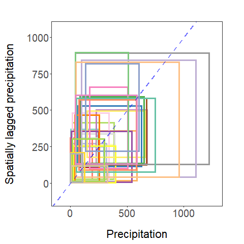
Figure 1: The Moran‘I Scatter plot of the centers (left) and the ranges (middle), the predicted precipitation versus the true values (right).

When only the ordinary single-valued data are invloved, spatial linear models, including spatial autoregressive model (SAR), spatial error model (SEM) and spatial Durbin model (SDM) are most commonly employed to analyze areal data. Through the utility of spatial weight matrix $\bm{W}$ and spatial lag parameter $\rho$, spatial models incorporates spatial effects into classic linear regressions. Estimation methods for these regressions cover quasi-maximum likelihood estimation method (Lee (2004)), generalized moment estimators (Lee (2007)) and the Markov Chain Monte Carlo (MCMC) method (Lesage and Pace (2009)). Their applications range from stock markets to social networks (Ma et al. (2020); Zhang et al. (2019)). As the SAR model is the most popular spatial model, we capitalize on it to struct our new model.

In this article, we propose a constrained spatial autoregressive model for interval-valued data (ICSM), which aims to predict interval-valued outcomes in the presence of areal-type spatial dependency. In particular, the CRM (center and range method) is utilized to handle inter-valued data. And we considered spatial correlation among centers of responses, employing the SAR model to form regression. We also take prediction accuracy into account by adding three inequality constrains in the model, motivated by Hao and Guo (2017). The parameters are obtained by the combination a grid search technique and the constrained least squares method. We also conduct numerical experiments to examine prediction performances of the proposed model. We find when spatial correlation is great and signal to noise is high, our model behaves better than models without spatial term and constrains. The weather data mentioned earlier is thoroughly analyzed by the new model.

We note that literatures related to spatial linear models of interval-valued data are relatively scanty. Han et al. (2016) discusses vector autoregressive moving average model for interval-valued data. Sun et al. (2018) proposes a new class of threshold autoregressive interval models. Although these investigations have considered correlation between intervals, they are mainly designed for interval-valued time series data, not interval-valued data with lattice-type spatial dependency.

The paper is organized as follows. Section 2 introduces the spatial autoregressive model and our proposed ICSM. Section 3 describes the algorithm to obtain the parameters. Numerical experiments are conducted in Section 4 to examine performances of the new model. Real data analysis are arranged in Section 5. We end up the article with a conclusion.

2 Model Specification

2.1 Spatial autoregressive (SAR) model

Ord (1975) proposed the spatial autoregressive (SAR) model, modeling spatial effects in the areal data. Suppose there are $n$ spatial units on a lattice, and each individual occupies a position. We observe $\{(x_{i},y_{i})\}_{i=1}^{n}$ from these entities. Denote $\bm{x}=\big{(}x_{1},x_{2},\cdots,x_{n}\big{)}^{\top}$ and $\bm{y}=(y_{1},y_{2},\cdots,y_{n})^{\top}$, the SAR model is formulated as

$$\bm{y}=\rho\bm{W}\bm{y}+\bm{x}\beta+\bm{\epsilon},~{}~{}~{}~{}\epsilon_{i}\sim N(0,\sigma^{2})$$

where $\bm{W}=(w_{ii^{\prime}})_{n\times n}$ is a spatial weight matrix, with each entry $w_{ii^{\prime}}$ representing the weight between unit $i$ and unit $i^{\prime}$, $\rho\in(-1,1)$ is the spatial lag parameter to be estimated, $\bm{\epsilon}=(\epsilon_{1},\cdots,\epsilon_{n})^{\top}$ is the noise term independent of $\bm{x}$ and i.i.d. following a normal distribution. $\beta$ is the scalar coefficient. Here, $\bm{W}$ quantifies spatial structure of the lattice, and the spatial lag term $\rho\bm{Wy}$ models spatial effects. The greater value $\rho$ takes, the stronger spatial impacts are imposed on $\bm{y}$.

It should be emphasized that generally $\bm{W}$ is exogenous and pre-specified, where $w_{ii^{\prime}}$ is determined by the contiguity or distance between $i$ and $i^{\prime}$ in different spatial scenarios. Rook matrix is among the most common spatial weight matrices, where

$$w_{ii^{\prime}}=\begin{cases}1,&i~{}and~{}i^{\prime}~{}share~{}an~{}edge\\ 0,&otherwise.\end{cases}$$

Bishop matrix is built in similar way by setting $w_{ii^{\prime}}=1$ when $i$ and $i^{\prime}$ have the same vertex. The key point to construct such matrix is knowing the map indicating spatial arrangement of the individuals. In case that geographical locations of spatial units are given, $w_{ii^{\prime}}$ can be functions of distance $d_{ii^{\prime}}$ between the two units, for example,

$$w_{ii^{\prime}}=\begin{cases}\frac{1}{d_{ii^{\prime}}},&d_{ii^{\prime}}\leq d_{0}\\ 0,&d_{ii^{\prime}}>d_{0}\end{cases}$$

where $d_{0}$ is a threshold distance. More general spatial weights can be derived from networks. For instance under a social network setting, $w_{ii^{\prime}}=1$ if person $i$ and $i^{\prime}$ are friends. For more information of $\bm{W}$, refer to Isard and et al (1970) and Anselin (1998). In general, $\bm{W}$ is row-normalized so that summation of the row elements is unity. Entries on the diagonal of $\bm{W}$ are zeros.

2.2 Constrained spatial autoregressive model for interval-valued data (ICSM)

Following Jenish and Prucha (2009), we presume the spatial process is located on an unevenly spaced lattice $L\in R^{n}~{}(n\geq 1)$, and all units on $L$ are endowed with positions ($L$ is crucial for establishing the weight matrix $\bm{W}$).

Denote an interval-valued variable as $\bm{w}^{s}=[w^{l},w^{u}]$, where $\bm{w}^{s}\in\mathcal{S}=\{[a,b]~{}\|~{}a,b\in\mathbb{R},a\leq b\}$. Here, we observe $\{\bm{y}_{i}^{s},\bm{x}_{i}^{s}\}_{i=1}^{n}$ from lattice $L$, and $\bm{y}_{i}^{s}=[y_{i}^{l},y_{i}^{u}],~{}\bm{x}_{i}^{s}=[x_{i}^{l},x_{i}^{u}]$. To deal with the interval-valued data, we employ the CRM method (Lima Neto and de Carvalho (2008)). Specifically, represent midpoint and radius of $\bm{w}^{s}$ by $w^{c}$ and $w^{r}$, and write $\bm{y}^{c}=(y_{1}^{c},\cdots,y_{n}^{c})^{\top},~{}\bm{y}^{r}=(y_{1}^{r},\cdots,y_{n}^{r})^{\top},~{}\bm{x}=(\bm{x}^{c},\bm{x}^{r})=((x_{1}^{c},\cdots,x_{n}^{c})^{\top},(x_{1}^{r},\cdots,x_{n}^{r})^{\top})$, then the constrained spatial autoregressive interval-valued model (ICSM) is formulated as

$$\begin{cases}\makebox[107.68912pt][l]{$\bm{y}^{c}=\rho\bm{Wy}^{c}+\bm{x}\bm{\beta}^{c}+\bm{\epsilon}^{c}$}&\\ \bm{y}^{r}=\bm{x}\bm{\beta}^{r}+\bm{\epsilon}^{r}&\end{cases}$$ (1)

$$s.t.\begin{cases}\makebox[107.68912pt][l]{$\bm{y}^{c}-\bm{y}^{r}\leq(\bm{I}_{n}-\rho\bm{W})^{-1}\cdot\bm{x\beta}^{c}+\bm{x\beta}^{r}$}&\\ \bm{y}^{c}+\bm{y}^{r}\geq(\bm{I}_{n}-\rho\bm{W})^{-1}\cdot\bm{x\beta}^{c}-\bm{x\beta}^{r}&\\ \bm{x\beta}^{r}\geq\bm{0}&\end{cases}$$

where $\bm{W}$ is the spatial weight matrix, $\rho\in(-1,1)$ is the spatial lag parameter, $\bm{\beta}^{c}=(\beta_{1}^{c},\beta_{2}^{c})$ and $\bm{\beta}^{r}=(\beta_{1}^{r},\beta_{2}^{r})$ are the coefficients, and $\bm{\epsilon}^{c}=(\epsilon^{c}_{1},\cdots,\epsilon^{c}_{n})^{\top},\bm{\epsilon}^{r}=(\epsilon^{r}_{1},\cdots,\epsilon^{r}_{n})^{\top}$ are the error terms with $E(\bm{\epsilon}^{c})=\bm{0},Var(\bm{\epsilon}^{c})=\sigma^{2}\bm{I}_{n},E(\bm{\epsilon}^{r})=\bm{0},Var(\bm{\epsilon}^{r})=\sigma^{2}\bm{I}_{n}$.

Note that compared to precisely forecast semi-length $\bm{y}^{r}$, accurately predicting mid-point $\bm{y}^{c}$ would contribute more to obtain a good predictor of $\bm{y}^{s}$. Therefore, considering simplicity and efficiency of the new model, we give priority to modeling spatial correlation of $\bm{y}^{c}$ by the SAR regression, fitting $\bm{y}^{r}$ by ordinary linear regression. We also considered effects from both centers and ranges of $\bm{x}^{s}$.

Inspired by Hao and Guo (2017), to improve prediction accuracy of the model, we add three inequality constraints to the interval-valued spatial regression, where the first two ensure predicted intervals have overlapping areas with the true values, and the last guarantees predicted value of $\bm{y}^{r}$ is positive. Concretely, in the first inequality, the forecasted upper bound of $\bm{y}^{s}$ should be greater than the observed lower bound of $\bm{y}^{s}$; and in the second, the forecasted lower bound of $\bm{y}^{s}$ should be smaller than the true upper bound of $\bm{y}^{s}$.

In model (5), $\rho$ quantifies average spatial effects among $\bm{y}^{s}$’s central positions. In particular, when $\rho=0$ the ICSM degenerates into the ICM (Hao and Guo (2017)). Thus (5) is a more general model.

3 Parameter estimation

Estimating $\rho,~{}\bm{\beta}^{c}$ and $\bm{\beta}^{r}$ of (5) is not straightforward due to the presence of spatial lag term $\rho\bm{Wy}^{c}$ and the constrains. Regarding $\rho$, commonly used methods to obtain it’s estimator include maximum likelihood estimation method (Lee (2004)), generalized moment estimators (Lee (2007)) and Markov Chain Monte Carlo method (Lesage and Pace (2009)). However, these approaches can not adapt to the situation that model parameters are restricted by inequalities. We put forward an algorithm that combines a grid search method with the constrained least squares to obtain estimators.

Firstly, as $\rho$ is a scalar number taking values from $-1$ to $1$, we can give a sufficiently fine grid of $m$ values for $\rho$. For example, take step size by $0.01$, then $m=201$ and $(\rho_{1},\rho_{2},\rho_{3},\cdots,\rho_{109},\rho_{200},\rho_{201})=(-1,-0.99,-0.98,\cdots,0.98,0.99,1)$.

Secondly, for each value of $\rho$, we solve a constrained least squares optimization problem. Provided value of $\rho_{j}~{}(j=1,\cdots,m)$, we can calculate

$$\bm{A}_{j}=(\bm{I}_{n}-\rho_{j}\bm{W}).$$

Then model (5) turns into

$$\left\{\begin{array}[]{ll}\bm{y}^{c}=\bm{A}_{j}^{-1}\cdot(\bm{x}\bm{\beta}^{c}+\bm{\epsilon}^{c})\\ \bm{y}^{r}=\bm{x}\bm{\beta}^{r}+\bm{\epsilon}^{r}\\ \end{array}\right.\quad s.t.\quad\left\{\begin{array}[]{ll}\bm{y}^{c}-\bm{y}^{r}\leq\bm{A}_{j}^{-1}\cdot\bm{x\beta}^{c}+\bm{x\beta}^{r}\\ \bm{y}^{c}+\bm{y}^{r}\geq\bm{A}_{j}^{-1}\cdot\bm{x\beta}^{c}-\bm{x\beta}^{r}\\ \bm{x\beta}^{r}\geq\bm{0}\\ \end{array}\right.$$

Now that $\bm{A}_{j}$ is known, we can employ least squares method to obtain $\hat{\bm{\beta}}^{c}$ and $\hat{\bm{\beta}}^{r}$. The sum of the squares of deviations is given by

$$\begin{split}&\min_{\bm{\beta}^{c},\bm{\beta}^{c}}\,~{}~{}(\bm{\epsilon}_{j}^{c})^{\top}\bm{\epsilon}_{j}^{c}+(\bm{\epsilon}_{j}^{r})^{\top}\bm{\epsilon}_{j}^{r}\\ &s.t.\quad\left\{\begin{array}[]{ll}-\bm{A}_{j}^{-1}\cdot\bm{x\beta}^{c}-\bm{x\beta}^{r}\leq-\bm{y}^{c}+\bm{y}^{r}\\ \bm{A}_{j}^{-1}\cdot\bm{x\beta}^{c}-\bm{x\beta}^{r}\leq\bm{y}^{c}+\bm{y}^{r}\\ -\bm{x\beta}^{r}\leq\bm{0}\\ \end{array}\right.\end{split}$$ (2)

where $\bm{\epsilon}_{j}^{c}=\bm{A}_{j}\cdot\bm{y}^{c}-\bm{x\beta}^{c}$ and $\bm{\epsilon}_{j}^{r}=\bm{y}^{r}-\bm{x\beta}^{r}$.

Once the solution for (2) is found for all candidates $\rho_{j}$, we select the $\rho_{j}$ with the least sum of square residuals as the $\hat{\rho}$. Accordingly, if the $j$th $\rho$ is the optimum $\rho$, then the $j$th estimated $\hat{\bm{\beta}}^{c}$ and $\hat{\bm{\beta}}^{r}$ are estimators of $\bm{\beta}^{c}$ and $\bm{\beta}^{r}$. We summarize the whole process in Algorithm 1.

Algorithm 1 Main steps of the estimation procedure

1:the dataset $\bm{y}^{c},\bm{y}^{r},\bm{x}^{c},\bm{x}^{r}$ and the spatial matrix $\bm{W}$.

2:Generate a sequence of $\rho$ from $-1$ to $1$ with step size $0.01$, that is $(\rho_{1},\cdots,\rho_{200},\rho_{201})=(-1,\cdots,0.99,1)$.

3:for $k=1$ to $201$ do

4:     compute $\bm{A}=\bm{I}_{n}-\rho_{k}\bm{W}$

5:     optimize

$$~{}~{}~{}\min\|\bm{Y}-\bm{Z\beta}\|^{2}~{}s.t.~{}\bm{G\beta}\leq\bm{h}~{}~{}~{}~{}$$

where $\bm{G}=\left(\begin{array}[]{cc}-\bm{A}^{-1}\bm{X}&-\bm{X}\\ \bm{A}^{-1}\bm{X}&-\bm{X}\\ \bm{0}_{n\times 3}&-\bm{X}\\ \end{array}\right),\bm{h}=\left(\begin{array}[]{c}\bm{y}^{r}-\bm{y}^{c}\\ \bm{y}^{c}+\bm{y}^{r}\\ \bm{0}_{n\times 1}\\ \end{array}\right),\bm{Z}=\left(\begin{array}[]{cc}\bm{X}&\bm{0}_{n\times 3}\\ \bm{0}_{n\times 3}&\bm{X}\\ \end{array}\right),\bm{Y}=\left(\begin{array}[]{c}\bm{Ay}^{c}\\ \bm{y}^{r}\\ \end{array}\right),~{}\bm{\beta}=\left(\begin{array}[]{c}\bm{\beta}_{1}\\ \bm{\beta}_{2}\\ \end{array}\right),~{}\bm{X}=\left(\begin{array}[]{ccc}\bm{I}_{n}&\bm{x}^{c}&\bm{x}^{r}\\ \end{array}\right),~{}\bm{\beta}_{1}=\left(\begin{array}[]{c}\beta_{0}^{c}\\ \bm{\beta}^{c}\\ \end{array}\right),~{}\bm{\beta}_{2}=\left(\begin{array}[]{c}\beta_{0}^{r}\\ \bm{\beta}^{r}\\ \end{array}\right)$.

6:end for

7:choose $\rho_{j}$ with the least $\|\bm{Y}-\bm{Z\beta}\|^{2}$, corresponding $\bm{\beta}$ is the estimated coefficient.

8:$\rho_{j}$ and the $j$th $\bm{\beta}$

4 simulation study

In this section, numerical experiments are conducted to show the superiority of our new method. Firstly, we introduce the data generating process. Secondly, we briefly explain how unobserved individuals are predicted under a spatial scenario. Two competing regression models are also considered. Lastly, we present several criterions to measure model performances and display the experimental results.

4.1 data generating process

For the spatial scenarios, we take two spatial weight matrices $\bm{W}$ into account, one is the commonly used rook matrix, and the other is the block matrix. These two matrices imply two cases of spatial structures, where the first corresponds to sparse networks, and the second corresponds to dense ones. More specifically, the spatial units under a rook scenario have a small number of neighbors, while the individuals under a block setting have a relatively greater number of neighbors. Here are details of generating the two matrices.

• Rook matrix assigns $w_{ii^{\prime}}=1$ if units $i$ and $i^{\prime}$ share an edge, and $w_{ii^{\prime}}=0$ otherwise. We assume $n$ agents are randomly located on a regular square lattice with $R$ rows and $T$ columns, where each agent occupies a cell. Then we have sample size $n=R\times T$. In this context, the agents have $4$ neighbors at most, and $2$ neighbors at least, given that they may be in the inner field or in the corner of the square grid. We set $n=\{10\texttimes 12,12\texttimes 20,20\texttimes 25\}=\{120,240,500\}$.

• Block matrix was first discussed by Case (1991), where there are $D$ number of districts, $M$ members in each district. Specifically, each unit $i$ in the block matrix has $m-1$ neighbors with equal weights, i.e., we set $w_{ii^{\prime}}=\frac{1}{m-1}$ if $i$ and $i^{\prime}$ are in the same district, $w_{ii^{\prime}}=0$ otherwise. We take $n=D\times M=\{20\times 6,20\times 12,25\times 20\}=\{120,240,500\}$

The numerical data are generated using the following model

$$\left\{\begin{array}[]{ll}\bm{y}^{c}&=(\bm{I}_{n}-\rho\bm{W})^{-1}\cdot(\bm{x}^{c}\beta_{1}^{c}+\bm{x}^{r}\beta_{2}^{c}+\bm{\epsilon}^{c})\\ \bm{y}^{r}&=\bm{x}^{c}\beta_{1}^{r}+\bm{x}^{r}\beta_{2}^{r}+\bm{\epsilon}^{r}\end{array}\right.$$

1. Regarding $\rho$, we consider three cases.

   1. $\rho=0$, where spatial dependency does not present. The ICSM degenerates into the CCRJM of Hao and Guo (2017).

   2. $\rho=0.4$, where network effects are moderate.

   3. $\rho=0.8$, where network effects are strong.

2. Centers and ranges of the interval covariates are generated by uniform distribution, i.e.

   $$\bm{x}^{c}\stackrel{{\scriptstyle i.i.d}}{{\sim}}U(0,150),~{}~{}~{}~{}~{}\bm{x}^{r}\stackrel{{\scriptstyle i.i.d}}{{\sim}}U(5,8)$$

3. Coefficients of the covariates $\beta_{1}^{c},\beta_{2}^{r}$ are generated by uniform distribution, as well

   $$\beta_{1}^{c}\sim U(-2.5,-2),~{}~{}~{}~{}~{}~{}\beta_{2}^{r}\sim U(2.5,5),~{}~{}~{}~{}~{}~{}\beta_{2}^{c}=1,~{}~{}~{}~{}\beta_{1}^{r}=0.1$$

4. To see how the prediction performance is influenced by different levels of noises of the center, we let

   1. $~{}~{}~{}\epsilon_{i}^{c}\sim U(0,11),~{}~{}~{}~{}\epsilon_{r}\sim U(0,5)$.

   2. $~{}~{}~{}\epsilon_{i}^{c}\sim U(0,18),~{}~{}~{}~{}\epsilon_{r}\sim U(0,5)$.

4.2 Predicting formula and comparative models

Note that in a spatial context, predicting $Y$ of an out-of-sample should be careful, as adding new observations will change the existing spatial structure, i.e., $\bm{W}$ is different. Goulard et al. (2017) studied the problem. They discussed out-of-sample prediction for the SAR model and concluded the “BP” predictor behaves well among other predictors. Denote in-sample observations by $(X_{s},Y_{s})$ and out-of-sample covariate by $X_{o}$, which are all known. Then the unknown out-of-sample response $Y_{o}$ can be calculated by “BP" predictor

$$\hat{Y}_{o}^{BP}=\hat{Y}_{o}^{TC}-Q_{o}^{-1}Q_{os}(Y_{s}-\hat{Y}_{s}^{TC})$$

$$\hat{Y}^{TC}=(I_{n}-\hat{\rho}W)^{-1}X\hat{\beta}=\begin{pmatrix}\hat{Y}_{s}^{TC}\\ \hat{Y}_{o}^{TC}\end{pmatrix}$$

$$Q=\frac{1}{\hat{\sigma}^{2}}(I_{n}-\hat{\rho}(W^{\top}+W)+\hat{\rho}^{2}W^{\top}W)=\begin{pmatrix}Q_{s}&Q_{so}\\ Q_{os}&Q_{o}\end{pmatrix}$$

where $\hat{\sigma}^{2}$ is mean square error of the fitting model. In our simulated data set, we randomly select $\frac{9}{10}n$ individuals as the learning set, and leave the remaining $\frac{1}{10}n$ units as the test set.

We compare the ICSM’s predictive power with other two models’: the constrained interval-valued model without spatial dependency (ICM), and the spatial interval-valued model without constrains (ISM), which can be formulated as

• The ICM (equivalent to the CCRJM by Hao and Guo (2017))

  $$\begin{cases}\makebox[148.6367pt][l]{$\bm{y}^{c}=\bm{x}^{c}\beta_{1}^{c}+\bm{x}^{r}\beta_{2}^{c}+\bm{\epsilon}^{c}$ }&\\ \bm{y}^{r}=\bm{x}^{c}\beta_{1}^{r}+\bm{x}^{r}\beta_{2}^{r}+\bm{\epsilon}^{r}\end{cases}$$ (3)

  $$s.t.\begin{cases}\makebox[148.6367pt][l]{$-(\bm{x}^{c}\beta_{1}^{c}+\bm{x}^{r}\beta_{2}^{c})-(\bm{x}^{c}\beta_{1}^{r}+\bm{x}^{r}\beta_{2}^{r})\leq-\bm{y}^{c}+\bm{y}^{r}$ }&\\ \bm{x}^{c}\beta_{1}^{c}+\bm{x}^{r}\beta_{2}^{c}-(\bm{x}^{c}\beta_{1}^{r}+\bm{x}^{r}\beta_{2}^{r})\leq\bm{y}^{c}+\bm{y}^{r}&\\ -(\bm{x}^{c}\beta_{1}^{r}+\bm{x}^{r}\beta_{2}^{r})\leq\bm{0}.&\end{cases}$$

• The ISM

  $$\left\{\begin{array}[]{ll}\bm{y}^{c}&=\rho\bm{Wy}^{c}+\bm{x}^{c}\beta_{1}^{c}+\bm{x}^{r}\beta_{2}^{c}+\bm{\epsilon}^{c}\\ \bm{y}^{r}&=\bm{x}^{c}\beta_{1}^{r}+\bm{x}^{r}\beta_{2}^{r}+\bm{\epsilon}^{r}.\end{array}\right.$$ (4)

4.3 measurements and comparison results

A number of criterion classes have been used to evaluate the performance of the interval linear regressions. Lim (2016) calculates root mean square error (RMSE) of the lower and upper bound of the predictive interval, i.e., RMSE_l and RMSE_u. Hojati et al. (2005) employs the accuracy rate (AR) to access similarity of two intervals based on the percentage of overlapping areas. We use these three criteria in our simulation, which are defined as

$$RMSE_{l}=\sqrt{\frac{1}{n}\sum_{i=1}^{n}(y_{i}^{l}-\hat{y}_{i}^{l})^{2}}$$

$$RMSE_{u}=\sqrt{\frac{1}{n}\sum_{i=1}^{n}(y_{i}^{u}-\hat{y}_{i}^{u})^{2}},$$

$$AR=\frac{1}{n}\sum_{i=1}^{n}\frac{\mu(\bm{y}_{i}\cap\hat{\bm{y}}_{i})}{\mu(\bm{y}_{i}\cup\hat{\bm{y}}_{i})},$$

where $\mu(\bm{y}_{i}\cap\hat{\bm{y}}_{i})$ and $\mu(\bm{y}_{i}\cup\hat{\bm{y}}_{i})$ are volumes of intersection and union of $\bm{y}_{i}$ and $\hat{\bm{y}_{i}}$, respectively.

Note that $AR$ is an average measurement of the overlapping areas. It may happen that the value of $AR$ is great, but some $\hat{\bm{y}_{i}}$ are mispredicted (the corresponding $\mu(\bm{y}_{i}\cap\hat{\bm{y}}_{i})$ equals $0$). To know how many individuals are wrongly forecasted in a data set, we add a new indicator $N_{d}$, which is the number of disjoint intervals, i.e.,

$$N_{d}=\#~{}\{i~{}\|~{}\mu(\bm{y}_{i}\cap\hat{\bm{y}}_{i})=0,~{}i=1,\cdots,n\}.$$

The whole process was repeated $75$ times in the experiment. We computed the average $MSE_{l},MSE_{u},AR,N_{d}$ and their standard deviations, summarized in Table 1 ($\rho=0$), Table 2 ($\rho=0.4$), and Table 3 ($\rho=0.8$).

Table 1: Prediction performances of ICSM, ICM and ISM when $\rho=0$.

			$MSE_{l}$				$MSE_{u}$
n	$\epsilon_{i}^{c}$	$\bm{W}$	ICSM	ICM	ISM		ICSM	ICM	ISM
120	N(0,11)	rook	$\underset{(2.0523)}{11.1014}$	$\underset{(2.0225)}{11.0722}$	$\underset{(2.1043)}{11.1052}$		$\underset{(2.2172)}{11.2156}$	$\underset{(2.1824)}{11.1783}$	$\underset{(2.2575)}{11.2237}$
		block	$\underset{(2.1504)}{11.2169}$	$\underset{(2.1351)}{11.1144}$	$\underset{(2.1985)}{11.2134}$		$\underset{(2.3606)}{11.2167}$	$\underset{(2.3259)}{11.0920}$	$\underset{(2.4171)}{11.2161}$
	N(0,18)	rook	$\underset{(3.5658)}{18.4828}$	$\underset{(3.5652)}{18.3768}$	$\underset{(3.5224)}{18.4603}$		$\underset{(3.4763)}{18.8141}$	$\underset{(3.4616)}{18.7145}$	$\underset{(3.4930)}{18.5812}$
		block	$\underset{(3.7560)}{18.4331}$	$\underset{(3.7507)}{18.4424}$	$\underset{(3.6357)}{18.4669}$		$\underset{(3.7473)}{18.3173}$	$\underset{(3.7632)}{18.3298}$	$\underset{(3.6742)}{18.3754}$
240	N(0,11)	rook	$\underset{(1.6740)}{11.0143}$	$\underset{(1.6876)}{11.0286}$	$\underset{(1.6674)}{11.0579}$		$\underset{(1.6481)}{11.1054}$	$\underset{(1.6549)}{11.1150}$	$\underset{(1.6442)}{11.1523}$
		block	$\underset{(1.4210)}{11.2274}$	$\underset{(1.4090)}{11.2125}$	$\underset{(1.4332)}{11.2541}$		$\underset{(1.4140)}{11.1916}$	$\underset{(1.4049)}{11.1743}$	$\underset{(1.4258)}{11.2184}$
	N(0,18)	rook	$\underset{(2.6180)}{18.1153}$	$\underset{(2.6334)}{18.1168}$	$\underset{(2.5155)}{17.9986}$		$\underset{(2.4520)}{17.9500}$	$\underset{(2.4717)}{17.9420}$	$\underset{(2.4846)}{17.9134}$
		block	$\underset{(3.2038)}{17.9657}$	$\underset{(3.1798)}{17.9348}$	$\underset{(3.0554)}{17.7945}$		$\underset{(3.2844)}{17.9281}$	$\underset{(3.2506)}{17.9095}$	$\underset{(3.1371)}{17.8560}$
500	N(0,11)	rook	$\underset{(0.9895)}{10.9784}$	$\underset{(0.9850)}{10.9739}$	$\underset{(0.9851)}{10.9848}$		$\underset{(0.9870)}{11.0429}$	$\underset{(0.9821)}{11.0348}$	$\underset{(0.9816)}{11.0498}$
		block	$\underset{(1.1267)}{10.9696}$	$\underset{(1.1224)}{10.9653}$	$\underset{(1.1257)}{10.9791}$		$\underset{(1.1408)}{11.0228}$	$\underset{(1.1370)}{11.0189}$	$\underset{(1.1387)}{11.0335}$
	N(0,18)	rook	$\underset{(1.7410)}{18.3842}$	$\underset{(1.7629)}{18.3787}$	$\underset{(1.6961)}{18.1039}$		$\underset{(1.7857)}{18.1269}$	$\underset{(1.7940)}{18.0955}$	$\underset{(1.6838)}{18.0033}$
		block	$\underset{(1.9952)}{18.5208}$	$\underset{(2.0078)}{18.5262}$	$\underset{(1.8678)}{18.2646}$		$\underset{(2.1360)}{18.4309}$	$\underset{(2.1583)}{18.4353}$	$\underset{(1.9304)}{18.3191}$
			$AR$				$N_{d}$
n	$\epsilon_{i}^{c}$	$\bm{W}$	ICSM	ICM	ISM		ICSM	ICM	ISM
120	N(0,11)	rook	$\underset{(0.0452)}{0.7749}$	$\underset{(0.0442)}{0.7748}$	$\underset{(0.0455)}{0.7747}$		$\underset{(0.0000)}{0.0000}$	$\underset{(0.0000)}{0.0000}$	$\underset{(0.0000)}{0.0000}$
		block	$\underset{(0.0441)}{0.7725}$	$\underset{(0.0435)}{0.7743}$	$\underset{(0.0448)}{0.7727}$		$\underset{(0.0000)}{0.0000}$	$\underset{(0.0000)}{0.0000}$	$\underset{(0.0000)}{0.0000}$
	N(0,18)	rook	$\underset{(0.0726)}{0.6453}$	$\underset{(0.0724)}{0.6467}$	$\underset{(0.0732)}{0.6446}$		$\underset{(0.2262)}{0.0533}$	$\underset{(0.2262)}{0.0533}$	$\underset{(0.4903)}{0.6133}$
		block	$\underset{(0.0687)}{0.6709}$	$\underset{(0.0691)}{0.6704}$	$\underset{(0.0682)}{0.6706}$		$\underset{(0.1155)}{0.0133}$	$\underset{(0.1155)}{0.0133}$	$\underset{(0.4957)}{0.5867}$
240	N(0,11)	rook	$\underset{(0.0388)}{0.7771}$	$\underset{(0.0390)}{0.7768}$	$\underset{(0.0386)}{0.7765}$		$\underset{(0.0000)}{0.0000}$	$\underset{(0.0000)}{0.0000}$	$\underset{(0.0000)}{0.0000}$
		block	$\underset{(0.0373)}{0.7693}$	$\underset{(0.0373)}{0.7695}$	$\underset{(0.0374)}{0.7687}$		$\underset{(0.0000)}{0.0000}$	$\underset{(0.0000)}{0.0000}$	$\underset{(0.0000)}{0.0000}$
	N(0,18)	rook	$\underset{(0.0541)}{0.6672}$	$\underset{(0.0538)}{0.6671}$	$\underset{(0.0552)}{0.6666}$		$\underset{(0.2731)}{0.0800}$	$\underset{(0.2731)}{0.0800}$	$\underset{(0.1622)}{0.9733}$
		block	$\underset{(0.0654)}{0.6696}$	$\underset{(0.0649)}{0.6703}$	$\underset{(0.0643)}{0.6703}$		$\underset{(0.0000)}{0.0000}$	$\underset{(0.0000)}{0.0000}$	$\underset{(0.4124)}{0.2133}$
500	N(0,11)	rook	$\underset{(0.0344)}{0.7755}$	$\underset{(0.0342)}{0.7756}$	$\underset{(0.0343)}{0.7755}$		$\underset{(0.0000)}{0.0000}$	$\underset{(0.0000)}{0.0000}$	$\underset{(0.0000)}{0.0000}$
		block	$\underset{(0.0326)}{0.7792}$	$\underset{(0.0325)}{0.7793}$	$\underset{(0.0325)}{0.7791}$		$\underset{(0.0000)}{0.0000}$	$\underset{(0.0000)}{0.0000}$	$\underset{(0.0000)}{0.0000}$
	N(0,18)	rook	$\underset{(0.0395)}{0.6711}$	$\underset{(0.0399)}{0.6712}$	$\underset{(0.0402)}{0.6719}$		$\underset{(0.2731)}{0.0800}$	$\underset{(0.2731)}{0.0800}$	$\underset{(0.0000)}{1.0000}$
		block	$\underset{(0.0469)}{0.6668}$	$\underset{(0.0470)}{0.6667}$	$\underset{(0.0467)}{0.6666}$		$\underset{(0.3661)}{0.1200}$	$\underset{(0.2929)}{0.0933}$	$\underset{(0.7884)}{1.2000}$

Table 2: Prediction performances of ICSM, ICM and ISM when $\rho=0.4$.

			$MSE_{l}$				$MSE_{u}$
n	$\epsilon_{i}^{c}$	$\bm{W}$	ICSM	ICM	ISM		ICSM	ICM	ISM
120	N(0,11)	rook	$\underset{(2.2722)}{11.4445}$	$\underset{(6.8898)}{26.8926}$	$\underset{(2.1702)}{11.4144}$		$\underset{(2.1354)}{11.4818}$	$\underset{(7.8028)}{27.2150}$	$\underset{(2.1127)}{11.4899}$
		block	$\underset{(2.3685)}{10.8221}$	$\underset{(6.7069)}{29.6401}$	$\underset{(2.3716)}{10.8411}$		$\underset{(2.1260)}{10.8115}$	$\underset{(6.1561)}{29.3916}$	$\underset{(2.1271)}{10.8306}$
	N(0,18)	rook	$\underset{(3.9168)}{18.1000}$	$\underset{(8.0248)}{32.3855}$	$\underset{(3.8590)}{18.1169}$		$\underset{(4.2566)}{18.3430}$	$\underset{(6.9920)}{31.0777}$	$\underset{(3.6878)}{18.1409}$
		block	$\underset{(3.2555)}{17.4380}$	$\underset{(8.8245)}{34.4353}$	$\underset{(3.2768)}{17.4085}$		$\underset{(3.2531)}{17.4482}$	$\underset{(7.6091)}{33.6160}$	$\underset{(3.2425)}{17.3586}$
240	N(0,11)	rook	$\underset{(1.5169)}{11.2280}$	$\underset{(4.8289)}{26.5330}$	$\underset{(1.5527)}{11.2390}$		$\underset{(1.5245)}{11.2742}$	$\underset{(5.2139)}{26.6516}$	$\underset{(1.5748)}{11.2438}$
		block	$\underset{(1.6397)}{11.0554}$	$\underset{(4.5317)}{22.5821}$	$\underset{(1.6432)}{11.0636}$		$\underset{(1.6779)}{10.9353}$	$\underset{(4.0878)}{22.0217}$	$\underset{(1.6815)}{10.9421}$
	N(0,18)	rook	$\underset{(3.0075)}{17.9222}$	$\underset{(7.0524)}{31.9797}$	$\underset{(2.6908)}{17.6607}$		$\underset{(3.0995)}{18.0094}$	$\underset{(6.6212)}{31.8204}$	$\underset{(2.6683)}{17.6132}$
		block	$\underset{(2.4087)}{17.6641}$	$\underset{(5.3542)}{27.5415}$	$\underset{(2.4046)}{17.5935}$		$\underset{(2.3808)}{17.6786}$	$\underset{(4.1114)}{26.2599}$	$\underset{(2.3896)}{17.5969}$
500	N(0,11)	rook	$\underset{(1.2764)}{11.4305}$	$\underset{(5.0379)}{28.5840}$	$\underset{(1.0681)}{11.2410}$		$\underset{(1.7726)}{11.5519}$	$\underset{(4.5871)}{28.0278}$	$\underset{(1.0960)}{11.2111}$
		block	$\underset{(1.1075)}{11.1313}$	$\underset{(2.4013)}{18.3621}$	$\underset{(1.1116)}{11.1339}$		$\underset{(1.1124)}{11.0830}$	$\underset{(2.4578)}{18.3696}$	$\underset{(1.1171)}{11.0864}$
	N(0,18)	rook	$\underset{(2.5031)}{18.7708}$	$\underset{(5.7933)}{33.8118}$	$\underset{(2.0405)}{18.0857}$		$\underset{(2.1667)}{18.3586}$	$\underset{(5.9500)}{34.6654}$	$\underset{(2.0512)}{18.0755}$
		block	$\underset{(2.3434)}{18.2823}$	$\underset{(4.3289)}{24.8806}$	$\underset{(2.2057)}{18.0818}$		$\underset{(2.1289)}{18.1978}$	$\underset{(3.1235)}{24.6113}$	$\underset{(2.1457)}{18.0764}$
			$AR$				$N_{d}$
n	$\epsilon_{i}^{c}$	$\bm{W}$	ICSM	ICM	ISM		ICSM	ICM	ISM
120	N(0,11)	rook	$\underset{(0.0526)}{0.7697}$	$\underset{(0.0994)}{0.5660}$	$\underset{(0.0521)}{0.7695}$		$\underset{(0.0000)}{0.0000}$	$\underset{(0.4124)}{0.2133}$	$\underset{(0.0000)}{0.0000}$
		block	$\underset{(0.0510)}{0.7795}$	$\underset{(0.0835)}{0.5363}$	$\underset{(0.0513)}{0.7791}$		$\underset{(0.0000)}{0.0000}$	$\underset{(0.3422)}{0.1333}$	$\underset{(0.0000)}{0.0000}$
	N(0,18)	rook	$\underset{(0.0719)}{0.6658}$	$\underset{(0.0836)}{0.5214}$	$\underset{(0.0720)}{0.6640}$		$\underset{(0.2262)}{0.0533}$	$\underset{(0.5012)}{0.2133}$	$\underset{(0.2929)}{0.9067}$
		block	$\underset{(0.0600)}{0.6761}$	$\underset{(0.0910)}{0.5075}$	$\underset{(0.0608)}{0.6769}$		$\underset{(0.0000)}{0.0000}$	$\underset{(0.4378)}{0.2533}$	$\underset{(0.0000)}{0.0000}$
240	N(0,11)	rook	$\underset{(0.0406)}{0.7738}$	$\underset{(0.0694)}{0.5728}$	$\underset{(0.0411)}{0.7737}$		$\underset{(0.0000)}{0.0000}$	$\underset{(0.3661)}{0.1200}$	$\underset{(0.0000)}{0.0000}$
		block	$\underset{(0.0402)}{0.7739}$	$\underset{(0.0701)}{0.6112}$	$\underset{(0.0402)}{0.7738}$		$\underset{(0.0000)}{0.0000}$	$\underset{(0.3108)}{0.1067}$	$\underset{(0.0000)}{0.0000}$
	N(0,18)	rook	$\underset{(0.0582)}{0.6755}$	$\underset{(0.0709)}{0.5365}$	$\underset{(0.0560)}{0.6780}$		$\underset{(0.2262)}{0.0533}$	$\underset{(0.6905)}{0.3600}$	$\underset{(0.1622)}{0.9733}$
		block	$\underset{(0.0513)}{0.6766}$	$\underset{(0.0655)}{0.5674}$	$\underset{(0.0522)}{0.6761}$		$\underset{(0.1155)}{0.0133}$	$\underset{(0.5774)}{0.2667}$	$\underset{(0.3691)}{0.8400}$
500	N(0,11)	rook	$\underset{(0.0406)}{0.7699}$	$\underset{(0.0581)}{0.5633}$	$\underset{(0.0374)}{0.7736}$		$\underset{(0.0000)}{0.0000}$	$\underset{(0.5733)}{0.3200}$	$\underset{(0.0000)}{0.0000}$
		block	$\underset{(0.0355)}{0.7732}$	$\underset{(0.0478)}{0.6658}$	$\underset{(0.0355)}{0.7732}$		$\underset{(0.0000)}{0.0000}$	$\underset{(0.3002)}{0.0667}$	$\underset{(0.0000)}{0.0000}$
	N(0,18)	rook	$\underset{(0.0467)}{0.6700}$	$\underset{(0.0653)}{0.5252}$	$\underset{(0.0463)}{0.6707}$		$\underset{(0.2929)}{0.0933}$	$\underset{(0.6595)}{0.4133}$	$\underset{(0.4027)}{1.0000}$
		block	$\underset{(0.0494)}{0.6670}$	$\underset{(0.0576)}{0.5922}$	$\underset{(0.0503)}{0.6673}$		$\underset{(0.3188)}{0.0800}$	$\underset{(0.5199)}{0.2000}$	$\underset{(1.0342)}{1.2267}$

Table 3: Prediction performances of ICSM, ICM and ISM when $\rho=0.8$.

			$MSE_{l}$				$MSE_{u}$
n	$\epsilon_{i}^{c}$	$\bm{W}$	ICSM	ICM	ISM		ICSM	ICM	ISM
120	N(0,11)	rook	$\underset{(9.6780)}{20.9170}$	$\underset{(46.9563)}{136.9090}$	$\underset{(2.6969)}{11.8538}$		$\underset{(13.6396)}{22.1827}$	$\underset{(43.4317)}{143.8223}$	$\underset{(2.7121)}{11.9363}$
		block	$\underset{(2.1735)}{10.0668}$	$\underset{(74.8370)}{268.4357}$	$\underset{(2.1649)}{10.0871}$		$\underset{(2.1566)}{10.1485}$	$\underset{(67.7378)}{276.4214}$	$\underset{(2.1272)}{10.1281}$
	N(0,18)	rook	$\underset{(11.7355)}{26.8112}$	$\underset{(38.1187)}{138.2213}$	$\underset{(4.1060)}{18.2134}$		$\underset{(11.7760)}{25.2355}$	$\underset{(44.4695)}{135.1789}$	$\underset{(3.8650)}{18.2767}$
		block	$\underset{(3.8754)}{17.7788}$	$\underset{(75.3455)}{276.9172}$	$\underset{(3.5006)}{17.5684}$		$\underset{(3.8585)}{18.1281}$	$\underset{(82.8051)}{286.9323}$	$\underset{(3.3895)}{17.6841}$
240	N(0,11)	rook	$\underset{(12.8142)}{22.5784}$	$\underset{(33.9702)}{145.8142}$	$\underset{(1.8895)}{11.5306}$		$\underset{(11.8816)}{22.3133}$	$\underset{(37.3522)}{155.3351}$	$\underset{(1.8967)}{11.4477}$
		block	$\underset{(1.5862)}{10.9630}$	$\underset{(53.9260)}{193.0556}$	$\underset{(1.5832)}{10.9685}$		$\underset{(1.5722)}{10.7834}$	$\underset{(51.5894)}{190.3062}$	$\underset{(1.5694)}{10.7810}$
	N(0,18)	rook	$\underset{(10.9487)}{29.6531}$	$\underset{(40.5606)}{167.7000}$	$\underset{(2.5728)}{17.4381}$		$\underset{(12.7241)}{32.8813}$	$\underset{(44.8410)}{165.4525}$	$\underset{(2.6281)}{17.4703}$
		block	$\underset{(2.9300)}{18.1834}$	$\underset{(43.7782)}{195.6656}$	$\underset{(2.6648)}{17.8889}$		$\underset{(2.6466)}{18.1563}$	$\underset{(56.4152)}{202.0845}$	$\underset{(2.5530)}{17.8429}$
500	N(0,11)	rook	$\underset{(14.5872)}{27.1713}$	$\underset{(37.4465)}{173.1929}$	$\underset{(1.1855)}{11.1199}$		$\underset{(13.2115)}{25.5140}$	$\underset{(33.4171)}{167.6693}$	$\underset{(1.1698)}{11.0789}$
		block	$\underset{(1.1800)}{11.0527}$	$\underset{(36.9454)}{147.2848}$	$\underset{(1.1786)}{11.0548}$		$\underset{(1.1966)}{11.1206}$	$\underset{(35.1845)}{142.7372}$	$\underset{(1.1941)}{11.1228}$
	N(0,18)	rook	$\underset{(10.7293)}{31.5665}$	$\underset{(35.4408)}{180.5881}$	$\underset{(1.6784)}{17.4332}$		$\underset{(12.5326)}{32.3119}$	$\underset{(32.0515)}{179.2781}$	$\underset{(1.6377)}{17.4337}$
		block	$\underset{(2.1603)}{18.2320}$	$\underset{(47.6102)}{163.7546}$	$\underset{(1.7004)}{17.7877}$		$\underset{(1.9119)}{17.9188}$	$\underset{(45.7619)}{161.2984}$	$\underset{(1.7644)}{17.8166}$
			$AR$				$N_{d}$
n	$\epsilon_{i}^{c}$	$\bm{W}$	ICSM	ICM	ISM		ICSM	ICM	ISM
120	N(0,11)	rook	$\underset{(0.1076)}{0.6513}$	$\underset{(0.0548)}{0.2094}$	$\underset{(0.0627)}{0.7540}$		$\underset{(0.0000)}{0.0000}$	$\underset{(0.6993)}{0.5867}$	$\underset{(0.0000)}{0.0000}$
		block	$\underset{(0.0503)}{0.7910}$	$\underset{(0.0314)}{0.1222}$	$\underset{(0.0502)}{0.7911}$		$\underset{(0.0000)}{0.0000}$	$\underset{(0.8246)}{0.6800}$	$\underset{(0.0000)}{0.0000}$
	N(0,18)	rook	$\underset{(0.0991)}{0.6168}$	$\underset{(0.0586)}{0.2234}$	$\underset{(0.0672)}{0.6769}$		$\underset{(0.1622)}{0.0267}$	$\underset{(0.8904)}{0.7333}$	$\underset{(0.4520)}{0.2800}$
		block	$\underset{(0.0683)}{0.6611}$	$\underset{(0.0331)}{0.1168}$	$\underset{(0.0692)}{0.6590}$		$\underset{(0.1155)}{0.0133}$	$\underset{(0.6443)}{0.5200}$	$\underset{(0.5030)}{0.4800}$
240	N(0,11)	rook	$\underset{(0.1138)}{0.6641}$	$\underset{(0.0444)}{0.2143}$	$\underset{(0.0406)}{0.7792}$		$\underset{(0.0000)}{0.0000}$	$\underset{(0.8268)}{0.5467}$	$\underset{(0.0000)}{0.0000}$
		block	$\underset{(0.0387)}{0.7811}$	$\underset{(0.0415)}{0.1660}$	$\underset{(0.0387)}{0.7811}$		$\underset{(0.0000)}{0.0000}$	$\underset{(0.7565)}{0.5733}$	$\underset{(0.0000)}{0.0000}$
	N(0,18)	rook	$\underset{(0.0914)}{0.5594}$	$\underset{(0.0433)}{0.1860}$	$\underset{(0.0558)}{0.6680}$		$\underset{(0.0000)}{0.0000}$	$\underset{(0.7236)}{0.4933}$	$\underset{(0.4452)}{0.7333}$
		block	$\underset{(0.0508)}{0.6730}$	$\underset{(0.0369)}{0.1602}$	$\underset{(0.0506)}{0.6748}$		$\underset{(0.1622)}{0.0267}$	$\underset{(0.7739)}{0.6800}$	$\underset{(0.5030)}{0.5200}$
500	N(0,11)	rook	$\underset{(0.1180)}{0.6192}$	$\underset{(0.0425)}{0.1867}$	$\underset{(0.0376)}{0.7738}$		$\underset{(0.0000)}{0.0000}$	$\underset{(0.6844)}{0.4667}$	$\underset{(0.0000)}{0.0000}$
		block	$\underset{(0.0357)}{0.7718}$	$\underset{(0.0439)}{0.2038}$	$\underset{(0.0357)}{0.7717}$		$\underset{(0.0000)}{0.0000}$	$\underset{(0.6611)}{0.5733}$	$\underset{(0.0000)}{0.0000}$
	N(0,18)	rook	$\underset{(0.0935)}{0.5617}$	$\underset{(0.0325)}{0.1746}$	$\underset{(0.0389)}{0.6768}$		$\underset{(0.1155)}{0.0133}$	$\underset{(0.7948)}{0.5067}$	$\underset{(0.2596)}{0.9867}$
		block	$\underset{(0.0462)}{0.6665}$	$\underset{(0.0468)}{0.1881}$	$\underset{(0.0456)}{0.6670}$		$\underset{(0.4638)}{0.1200}$	$\underset{(0.7493)}{0.6267}$	$\underset{(0.6513)}{1.1867}$

5 Application

In this section, we give a detailed analysis of the weather data mentioned in Section 1 using the proposed new model. In particular, to examine the prediction power of the ICSM, we collected monthly temperature and monthly rainfall data in the year of $2020$ from China Meteorological Yearbook. That is, data in $2019$ acts as training set, and those in $2020$ acts as test set. In the preprocessing of the data, we first take logarithm of the precipitation, then group all the single values into intervals. The ICSM is built as

$$\left\{\begin{array}[]{ll}y_{i}^{c}=\rho\sum_{i^{\prime}\neq i}w_{ii^{\prime}}y_{i^{\prime}}+x_{i}^{c}\beta_{1}^{c}+x_{i}^{r}\beta_{2}^{c}+\epsilon_{i}^{c}\\ y_{i}^{r}=x_{i}^{c}\beta_{1}^{r}+x_{i}^{r}\beta_{2}^{r}+\epsilon_{i}^{r}\end{array}\right.$$

$$s.t.\quad\left\{\begin{array}[]{ll}y_{i}^{c}-\rho\sum_{i^{\prime}\neq i}w_{ii^{\prime}}y_{i^{\prime}}-y_{i}^{r}\leq x_{i}^{c}\beta_{1}^{c}+x_{i}^{r}\beta_{2}^{c}+x_{i}^{c}\beta_{1}^{r}+x_{i}^{r}\beta_{2}^{r}\\ y_{i}^{c}-\rho\sum_{i^{\prime}\neq i}w_{ii^{\prime}}y_{i^{\prime}}+y_{i}^{r}\geq x_{i}^{c}\beta_{1}^{c}+x_{i}^{r}\beta_{2}^{c}-(x_{i}^{c}\beta_{1}^{r}+x_{i}^{r}\beta_{2}^{r})\\ x_{i}^{c}\beta_{1}^{r}+x_{i}^{r}\beta_{2}^{r}\geq 0.\\ \end{array}\right.$$

And the ICM is

$$\left\{\begin{array}[]{ll}y_{i}^{c}=x_{i}^{c}\beta_{1}^{c}+x_{i}^{r}\beta_{2}^{c}+\epsilon_{i}^{c}\\ y_{i}^{r}=x_{i}^{c}\beta_{1}^{r}+x_{i}^{r}\beta_{2}^{r}+\epsilon_{i}^{r}\end{array}\right.\quad s.t.\quad\left\{\begin{array}[]{ll}y_{i}^{c}-y_{i}^{r}\leq x_{i}^{c}\beta_{1}^{c}+x_{i}^{r}\beta_{2}^{c}+x_{i}^{c}\beta_{1}^{r}+x_{i}^{r}\beta_{2}^{r}\\ y_{i}^{c}+y_{i}^{r}\geq x_{i}^{c}\beta_{1}^{c}+x_{i}^{r}\beta_{2}^{c}-(x_{i}^{c}\beta_{1}^{r}+x_{i}^{r}\beta_{2}^{r})\\ x_{i}^{c}\beta_{1}^{r}+x_{i}^{r}\beta_{2}^{r}\geq 0.\\ \end{array}\right.$$ (5)

where $y_{i}^{c},~{}y_{i}^{r}$ are center and radius of the interval-valued precipitation of city $i$, $x_{i}^{c}$ and $x_{i}^{r}$ are mid-point and semi-length of the interval-valued temperature of city $i$, $w_{ii^{\prime}}$ is the spatial weight between cities $i$ and $i^{\prime}$. $\rho,\beta_{1}^{c},\beta_{2}^{c},\beta_{1}^{r},\beta_{2}^{r}$ are parameters to be estimated.

In model 5, we utilize the inverse distance to obtain $w_{ii^{\prime}}$, i.e., $w_{ii^{\prime}}=\frac{1}{d_{ii^{\prime}}}$, where $d_{ii^{\prime}}$ is the distance between cities $i$ and $i^{\prime}$ computed by longitudes and latitudes. Figure LABEL: displays locations of these cities on map of China. To determine a proper $\bm{W}$ for the ICSM, we consider two factors. The first is the number of neighbors $k$, which determines the sparsity of $\bm{W}$. The second is the distance threshold $d_{0}$. It is known that the greater the $d_{ii^{\prime}}$, the weaker the spatial effects. Thus we set $w_{ii^{\prime}}=0$ if $d_{ii^{\prime}}>d_{0}$, and $\frac{1}{d_{ii^{\prime}}}$ otherwise. To choose an optimal pair of $(k,d_{0})$ for $\bm{W}$, we firstly set $k=\{1,2,3,\cdots,9\}$. Then regarding each $k$, search for a $d_{0}$, which makes the Moran’s I statistic of $\bm{y}^{c}$ take the greatest value. Table 4 shows results for $k$ and $d_{0}$. It can bee seen that $k=2$ with $d_{0}=492.37$ km is the best choice.

Table 4: Values of the Moran’s I statistics of $y_{i}^{c}$s when $k=\{1,2,3,\cdots,9\}$.

$k$	$1$	$2$	$3$	$4$	$5$	$6$	$7$	$8$	$9$
Moran’s I	0.678	0.687	0.636	0.641	0.643	0.648	0.646	0.646	0.646
$d_{0}$ (km)	446.57	492.37	492.37	492.37	492.37	492.37	492.37	492.37	492.37

Table 5 compares the ICSM and the ICM in terms of both fitting and prediction performances. It is obvious that the ICSM behaves better than the ICM. We can see spatial dependencies are eliminated in the residuals of the ICSM (with the Moran’s I statistic being $-0.24$), while still present in those of the ICM (with the Moran’s I statistic being $0.46$). From Figure 2 (left and middle) we can come to similar conclusion, which displays Moran’s I scatter plots of the residuals. Besides, MSE of the residuals of the ICSM is $0.580$, smaller than that of the ICM ($0.674$). Regarding prediction performance, the ICSM has wider overlapping areas ($44.23\%$) than the ICM ($43.96\%$) by average, and smaller forecast errors of the lower and the upper bounds of the precipitation intervals. Figure 2 (right) exhibits predicted intervals versus the real values.

Table 5: Fitting and prediction results of the ICSM and the ICM.

Models	Moran’s I statistic (residuals of $y_{i}^{c}$s)	MSE (fitt ed error)	MSE (predi ction error)	AR	MSEl	MSEu
ICSM	-0.24 (0.901)	0.580	0.668	44.23%	0.790	0.519
ICM	0.46 (0.002)	0.674	0.712	43.96%	0.822	0.583

Table 6 summarizes estimation results of the ICSM and the ICM. The spatial lag parameter $\hat{\rho}$ is $0.56$, meaning spatial effects in the precipitation are medium. $\hat{\beta}_{1}^{c}$ and $\hat{\beta}_{2}^{c}$ are equivalent to $0.261$ and $0.195$, respectively, thus $y_{i}^{c}$s are positively related to both centers and ranges of the temperatures. However, $\hat{\beta}_{1}^{r}$ equals $0.108$ and $\hat{\beta}_{2}^{r}$ is $-0.003$, indicating $y_{i}^{r}$s are mainly influenced by mid-points of the temperatures. And semi-lengths of the temperatures play a relatively small role.

Table 6: The fitting results of the ICSM and the ICM.

models	$\hat{\rho}$	$\hat{\beta}_{0}^{c}$	$\hat{\beta}_{1}^{c}$	$\hat{\beta}_{2}^{c}$	$\hat{\beta}_{0}^{r}$	$\hat{\beta}_{1}^{r}$	$\hat{\beta}_{2}^{r}$
ICSM	0.56	-0.167	0.261	0.195	0.710	0.108	-0.003
ICM	—	-0.250	0.510	0.284	0.710	0.108	-0.003

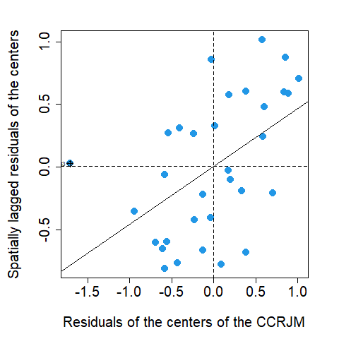
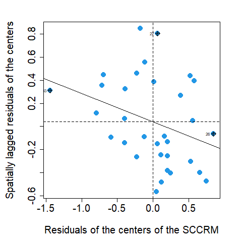
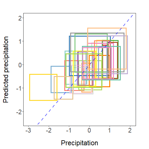
Figure 2: The Moran’I Scatter plot of the residuals of $y_{i}^{c}$s in the ICM (left) and the ICSM (middle), the predicted $2020$ precipitation intervals versus the true values using the ICSM (right).

6 Conclusion

Interval-valued data receives much attention due to it’s wide applications in the area of meteorology, medicine, finance, etc. Regression models concentrated on this kind of data have also been extended to nonparametric paradigms and the Bayesian framework. Nevertheless, relative few literature considered spatial dependence among intervals. In the article, we put forward a constrained spatial autoregressive model (ICSM) to model interval-valued data with lattice-type spatial correlation. In particular, for the simplicity and efficiency of the new model, we only take spatial effects among centers of responses into account. And to improve prediction accuracy of the model, three inequality constrains for the parameters are added. We obtain the parameters by a grid search technique combined with the constrained least-squares method. Simulation studies show that our new model behaves better than the model without spatial lag term (ICM) and the model without constrains (ISM), when spatial dependencies are present and disturbances are great. And in cases that there are no spatial correlation or disturbances are small, our model performs similarly with the other two models. We also employ a real dataset of temperatures and precipitation to illustrate the utility of the ICSM.

Although we only considered spatial effects among mid-points of outcomes, spatial correlation among the semi-lengths can also be took into consideration by adding a spatial lag term in the linear regression. Under this new model with two different spatial lag parameters, estimator can be gotten by the addition of a “for” loop, which searches for an adequate $\rho^{r}$ for $\bm{y}^{r}$. Note that the additional iteration would greatly increase the computation time. In future, we will discuss more flexible models, such as the incorporation of two different spatial weight matrices, and more general assumptions of the noise terms.

References

• \bibcommenthead
• Anselin (1998) Anselin, L. 1998. Spatial Econometrics: Methods and Models. Springer Science & Business Media.
• Billard and Diday (2002) Billard, L. and E. Diday. 2002. Symbolic Regression Analysis, In Classification, Clustering, and Data Analysis, eds. Bock, H.H., W. Gaul, M. Schader, K. Jajuga, A. Sokołowski, and H.H. Bock, 281–288. Berlin, Heidelberg: Springer Berlin Heidelberg. Series Title: Studies in Classification, Data Analysis, and Knowledge Organization. 10.1007/978-3-642-56181-8_31.
• Billard and Diday (2003) Billard, L. and E. Diday. 2003, June. From the Statistics of Data to the Statistics of Knowledge: Symbolic Data Analysis. Journal of the American Statistical Association 98(462): 470–487. 10.1198/016214503000242 .
• Case (1991) Case, A.C. 1991. Spatial Patterns in Household Demand. Econometrica 59(4): 953–965. 10.2307/2938168 .
• de Carvalho et al. (2021) de Carvalho, F.d.A., E.d.A. Lima Neto, and K.C. da Silva. 2021, May. A clusterwise nonlinear regression algorithm for interval-valued data. Information Sciences 555: 357–385. 10.1016/j.ins.2020.10.054 .
• Diday (1988) Diday, E. 1988. The symbolic approach in clustering and related methods of data analysis: The basic choices. In Proceedings of IFCS’87 on Classification and Related Methods of Data Analysis, pp.  673–684.
• Fagundes et al. (2014) Fagundes, R.A., R.M. de Souza, and F.J.A. Cysneiros. 2014, March. Interval kernel regression. Neurocomputing 128: 371–388. 10.1016/j.neucom.2013.08.029 .
• Goulard et al. (2017) Goulard, M., T. Laurent, and C. Thomas-Agnan. 2017. About predictions in spatial autoregressive models: optimal and almost optimal strategies. Spatial Economic Analysis 12(2-3): 304–325. 10.1080/17421772.2017.1300679. https://doi.org/10.1080/17421772.2017.1300679 .
• Han et al. (2016) Han, A., Y. Hong, S. Wang, and X. Yun. 2016, June. A Vector Autoregressive Moving Average Model for Interval-Valued Time Series Data, In Advances in Econometrics, eds. GonzÁlez-Rivera, G., R.C. Hill, and T.H. Lee, Volume 36, 417–460. Emerald Group Publishing Limited. 10.1108/S0731-905320160000036021.
• Hao and Guo (2017) Hao, P. and J. Guo. 2017, December. Constrained center and range joint model for interval-valued symbolic data regression. Computational Statistics & Data Analysis 116: 106–138. 10.1016/j.csda.2017.06.005 .
• Hojati et al. (2005) Hojati, M., C. Bector, and K. Smimou. 2005. A simple method for computation of fuzzy linear regression. European Journal of Operational Research 166(1): 172–184. 10.1016/j.ejor.2004.01.039 .
• Isard and et al (1970) Isard, W. and et al. 1970. General theory: social, political, economic and regional. Cambridge, Mass./London: Mass. Inst. Technol.
• Jenish and Prucha (2009) Jenish, N. and I.R. Prucha. 2009. Central limit theorems and uniform laws of large numbers for arrays of random fields. Journal of Econometrics 150(1): 86 – 98. https://doi.org/10.1016/j.jeconom.2009.02.009 .
• Lee (2004) Lee, L.f. 2004. Asymptotic Distributions of Quasi-Maximum Likelihood Estimators for Spatial Autoregressive Models. Econometrica 72(6): 1899–1925. 10.1111/j.1468-0262.2004.00558.x. https://onlinelibrary.wiley.com/doi/pdf/10.1111/j.1468-0262.2004.00558.x .
• Lee (2007) Lee, L.f. 2007. GMM and 2SLS estimation of mixed regressive, spatial autoregressive models. Journal of Econometrics 137(2): 489–514. https://doi.org/10.1016/j.jeconom.2005.10.004 .
• Lesage and Pace (2009) Lesage, J. and R.K. Pace. 2009. Introduction to Spatial Econometrics. Chapman and Hall/CRC.
• Lim (2016) Lim, C. 2016, September. Interval-valued data regression using nonparametric additive models. Journal of the Korean Statistical Society 45(3): 358–370. 10.1016/j.jkss.2015.12.003 .
• Lima Neto and de Carvalho (2008) Lima Neto, E.d.A. and F.d.A. de Carvalho. 2008, January. Centre and Range method for fitting a linear regression model to symbolic interval data. Computational Statistics & Data Analysis 52(3): 1500–1515. 10.1016/j.csda.2007.04.014 .
• Lima Neto and de Carvalho (2010) Lima Neto, E.d.A. and F.d.A. de Carvalho. 2010, February. Constrained linear regression models for symbolic interval-valued variables. Computational Statistics & Data Analysis 54(2): 333–347. 10.1016/j.csda.2009.08.010 .
• Lima Neto and de Carvalho (2018) Lima Neto, E.d.A. and F.d.A. de Carvalho. 2018, July. An exponential-type kernel robust regression model for interval-valued variables. Information Sciences 454-455: 419–442. 10.1016/j.ins.2018.05.008 .
• Lima Neto and de Carvalho (2017) Lima Neto, E.d.A. and F.d.A.T. de Carvalho. 2017, August. Nonlinear regression applied to interval-valued data. Pattern Analysis and Applications 20(3): 809–824. 10.1007/s10044-016-0538-y .
• Ma et al. (2020) Ma, Y., R. Pan, T. Zou, and H. Wang. 2020. A Naive Least Squares Method for Spatial Autoregression with Covariates. Statistica Sinica. 10.5705/ss.202017.0135 .
• Ord (1975) Ord, K. 1975. Estimation methods for models of spatial interaction. Journal of the American Statistical Association 70(349): 120–126. 10.1080/01621459.1975.10480272 .
• Sun et al. (2022) Sun, L., L. Zhu, W. Li, C. Zhang, and T. Balezentis. 2022, August. Interval-valued functional clustering based on the Wasserstein distance with application to stock data. Information Sciences 606: 910–926. 10.1016/j.ins.2022.05.112 .
• Sun (2016) Sun, Y. 2016, January. Linear regression with interval-valued data: Linear regression with interval-valued data. Wiley Interdisciplinary Reviews: Computational Statistics 8(1): 54–60. 10.1002/wics.1373 .
• Sun et al. (2018) Sun, Y., A. Han, Y. Hong, and S. Wang. 2018, October. Threshold autoregressive models for interval-valued time series data. Journal of Econometrics 206(2): 414–446. 10.1016/j.jeconom.2018.06.009 .
• Topa (2001) Topa, G. 2001. Social Interactions, Local Spillovers and Unemployment. The Review of Economic Studies 68(2): 261–295. 10.1111/1467-937X.00169 .
• Wang et al. (2012) Wang, H., R. Guan, and J. Wu. 2012, June. CIPCA: Complete-Information-based Principal Component Analysis for interval-valued data. Neurocomputing 86: 158–169. 10.1016/j.neucom.2012.01.018 .
• Wei et al. (2017) Wei, Y., S. Wang, and H. Wang. 2017, August. Interval-valued data regression using partial linear model. Journal of Statistical Computation and Simulation: 1–20. 10.1080/00949655.2017.1360298 .
• Xu and Qin (2022) Xu, M. and Z. Qin. 2022, January. A bivariate Bayesian method for interval-valued regression models. Knowledge-Based Systems 235: 107396. 10.1016/j.knosys.2021.107396 .
• Yang et al. (2019) Yang, Z., D.K. Lin, and A. Zhang. 2019, February. Interval-valued data prediction via regularized artificial neural network. Neurocomputing 331: 336–345. 10.1016/j.neucom.2018.11.063 .
• Zhang et al. (2019) Zhang, W., X. Zhuang, and Y. Li. 2019, December. Spatial spillover around G20 stock markets and impact on the return: a spatial econometrics approach. Applied Economics Letters 26(21): 1811–1817. 10.1080/13504851.2019.1602703 .