Improvement-Focused Causal Recourse (ICR)

Abstract

Algorithmic recourse recommendations, such as Karimi et al.’s (2021) causal recourse (CR), inform stakeholders of how to act to revert unfavorable decisions. However, there are actions that lead to acceptance (i.e., revert the model’s decision) but do not lead to improvement (i.e., may not revert the underlying real-world state). To recommend such actions is to recommend fooling the predictor. We introduce a novel method, Improvement-Focused Causal Recourse (ICR), which involves a conceptual shift: Firstly, we require ICR recommendations to guide towards improvement. Secondly, we do not tailor the recommendations to be accepted by a specific predictor. Instead, we leverage causal knowledge to design decision systems that predict accurately pre- and post-recourse. As a result, improvement guarantees translate into acceptance guarantees. We demonstrate that given correct causal knowledge ICRguides towards both acceptance and improvement.

Keywords algorithmic recourse  $\cdot$ gaming  $\cdot$ causal inference  $\cdot$ interpretable machine learning  $\cdot$ robustness

1 Introduction

Predictive systems are increasingly deployed for high-stakes decisions, for instance in hiring (Raghavan et al., 2020), judicial systems (Zeng et al., 2017), or when distributing medical resources (Obermeyer and Mullainathan, 2019). A range of work (Wachter et al., 2017; Ustun et al., 2019; Karimi et al., 2021) develops tools that offer individuals possibilities for so-called algorithmic recourse (i.e. actions that revert unfavorable decisions). Joining previous work in the field, we distinguish between reverting the model’s prediction $\hat{Y}$ (acceptance) and reverting the underlying real-world state $Y$ (improvement) and argue that recourse should lead to acceptance and improvement (Ustun et al., 2019; Barocas et al., 2020). Existing methods, such as counterfactual explanations (CE; Wachter et al. (2017)) or causal recourse (CR; Karimi et al. (2021)), ignore the underlying real-world state and only optimize for acceptance. Since ML models are not designed to predict accurately in interventional environments (i.e. environments where actions have changed the data distribution), acceptance does not necessarily imply improvement.
Let us consider a simple motivational example. The goal is to predict whether hospital visitors without recent test certificate are infected with Covid in order to restrict access to tested and low-risk individuals. In the example, the model’s prediction $\hat{Y}$ represents whether someone is classified to be infected, whereas the prediction target $Y$ represents whether someone is actually infected. Target and prediction differ in how they are affected by actions. E.g., intervening on the symptoms may change the diagnosis $\hat{Y}$, but will not affect whether someone is infected ($Y$).
Both counterfactual explanations (CE) and causal recourse (CR) only target $\hat{Y}$ (Figure 1). Therefore, CE and CR may suggest to alter the symptoms (e.g., by taking cough drops) and thereby may recommend to game the predictor: Although the intervention leads to acceptance the actual Covid risk $Y$ is not improved.

Figure 1: Directed Acyclic Graph (DAG) illustrating the perspective on model and data taken by counterfactual explanations (CE, left) and causal recourse (CR, center) in contrast to improvement-focused recourse (ICR, right). Blue edges represent the causal links induced by the prediction model, green edges the real-world causal links, gray nodes the covariates, and the red (yellow) node the primary (secondary) recourse target. CR respects the causal relationships but only between input features. ICR is the only approach that takes the target $Y$ into account. While CE and CR aim to revert the prediction $\hat{Y}$, ICR aims to revert the target $Y$.

One may argue that this is an issue of the prediction model and may adapt the predictor strategically to make gaming less lucrative than improvement (Miller et al., 2020). In our example, the model’s reliance on the symptom state would need to be reduced. However, such strategic adaptions may come at the cost of predictive performance since gameable variables, like the symptom state, can be highly predictive (Shavit et al., 2020). Thus, we tackle the problem by adjusting the explanation.

Contributions

We present improvement-focused causal recourse (ICR), the first recourse method that targets improvement instead of acceptance. Since estimating the effects of actions is a causal problem, causal knowledge is required. More specifically, we show how to exploit either knowledge of the structural causal model (SCMs) or the causal graph to guide towards improvement (Section 5). On a conceptual level we argue that the individual’s improvement options should not be limited by an acceptance constraint (Section 4). In order to nevertheless yield acceptance, we show how to exploit said causal knowledge to design post-recourse decision systems that in expectation recognize improvement (Section 6), such that improvement guarantees translate into acceptance guarantees (Section 7). On synthetic and semi-synthetic data, we demonstrate that ICR, in contrast to existing approaches, leads to improvement and acceptance (Section 8).

2 Related Work

Constrastive Explanations

Contrastive explanations explain decisions by contrasting them with alternative decision scenarios (Karimi et al., 2020a; Stepin et al., 2021); a well known example are counterfactual explanations (CE) that highlight the minimal feature changes required to revert the decision of a predictor $\hat{f}(x)$ (Wachter et al., 2017; Dandl et al., 2020). However, CEs are ignorant of causal dependencies in the data and therefore in general fail to guide action (Karimi et al., 2021). In contrast, the causal recourse (CR) framework by Karimi et al. (2022) takes the causal dependencies between covariates into account: More specifically, Karimi et al. (2022) use structural causal models or causal graphs to guide individuals towards acceptance. The importance of improvement was discussed before (Ustun et al., 2019; Barocas et al., 2020), but as of now no improvement-focused recourse method was proposed.

Strategic Classification

The related field of strategic modeling investigates how the prediction mechanism incentivizes rational agents (Hardt et al., 2016; Tsirtsis and Gomez Rodriguez, 2020). A range of work (Bechavod et al., 2020; Chen et al., 2020; Miller et al., 2020) thereby distinguishes models that incentivize gaming (i.e., interventions that affect the prediction $\hat{Y}$ but not the underlying target $Y$ in the desired way) and improvement (i.e., actions that also yield the desired change in $Y$). Strategic modeling is concerned with adapting the model, where except for special cases the following three goals are in conflict: incentivizing improvement, predictive accuracy, and retrieving the true underlying mechanism (Shavit et al., 2020).

Robust algorithmic recourse

The robustness of CEs and CR has been investigated before (Rawal et al., 2021; Pawelczyk et al., 2020; Upadhyay et al., 2021; Dominguez-Olmedo et al., 2021; Pawelczyk et al., 2022), yet only with respect to generic shifts of model and data. Only Pawelczyk et al. (2020) investigate the robustness regarding refits on the same data. They find that on-the-manifold CEs are more robust than standard CEs. In contrast, we empirically compare the robustness of CE, CR and ICR with respect to refits on the same data.

3 Background and Notation

Prediction model

We assume binary probabilistic predictors and cross-entropy loss, such that the optimal score function $h^{*}(x)$ models the conditional probability $P(Y=1|X=x)$, which we abbreviate as $p(y|x)$. We denote the estimated score function as $\hat{h}(x)$, which can be transformed into the binary decision function $\hat{f}(x):=[\hat{h}(x)\geq t]$ via the decision threshold $t$.

Causal data model

We model the data generating process using a structural causal model (SCM) $\mathcal{M}\in\Pi$ (Pearl, 2009; Peters et al., 2017). The model $\mathcal{M}=\langle X,U,\mathbb{F}\rangle$ consists of the endogenous variables $X\in\mathcal{X}$, the mutually independent exogenous variables $U\in\mathcal{U}$, and structural equations $\mathbb{F}:\mathcal{U}\to\mathcal{X}$. Each structural equation $f_{j}$ specifies how $X_{j}$ is determined by its endogenous causes and the corresponding exogenous variable $U_{j}$. The SCM entails a directed graph $\mathcal{G}$, where variables are connected to their direct effects via a directed edge.
The index set of endogenous variables is denoted as $D$. The parent indexes of node $j$ are referred to as $pa(j)$ and the children indexes as $ch(j)$. We refer to the respective variables as $X_{pa(j)}$. We write $X_{pa(j)}$ to denote all parents excluding $Y$ and $(X,Y)_{pa(j)}$ to denote all parents including $Y$. All ascendant indexes of a set $S$ are denoted as $asc(S)$, its complement as $nasc(S)$, all descendant indexes as $d(S)$, and its complement as $nd(S)$.
SCMs allow to answer causal questions. This means that they cannot only be used to describe (conditional) distributions (observation, rung 1 on Pearl’s ladder of causation (Pearl, 2009)), but can also be used to predict the (average) effect of actions $do(x)$ (intervention, rung 2) and imagine the results of alternative actions in light of factual observation $(x,y)^{F}$ (counterfactuals, rung 3).
As such, we model actions as structural interventions $a:\Pi\to\Pi$, which can be constructed as $do(a)=do(\{X_{i}:=\theta_{i}\}_{i\in I})$, where $I$ is the index set of features to be intervened upon. A model of the interventional distribution can be obtained by fixing the intervened upon values to $\theta_{I}$ (e.g. by replacing the structural equation $f_{I}:=\theta_{I}$). Counterfactuals can be computed in three steps (Pearl, 2009): First, the factual distribution of exogenous variables $U$ given the factual observation of the endogenous variables $x^{F}$ is inferred (abduction) (i.e., $P(U_{j}|X^{F})$). Second, the structural interventions corresponding to $do(a)$ are performed (action). Finally, we can sample from the counterfactual distribution $P(X^{SCF}|X=x^{F},do(a))$ using the abducted noise and the intervened-upon structural equations (prediction).

4 The Two Tales of Contrastive Explanations

In the introduction we have demonstrated that CE and CR may suggest to game the predictor (i.e. guide towards acceptance without improvement). To tackle the issue, we will introduce a new explanation technique called improvement-focused causal recourse (ICR) in Section 5.
In this section we lay the conceptual justification for our method. More specifically, we argue that for recourse the acceptance constraint of CR should be replaced by an improvement constraint. Therefore, we first recall that a multitude of goals may be pursued with contrastive explanations (Wachter et al., 2017) and separate two purposes of contrastive explanations: contestability of algorithmic decisions and actionable recourse. We then argue that improvement is an essential requirement for recourse and that the individual’s options for improvement should not be limited by acceptance constraints.

Contestability and recourse are distinct goals.

Contestability is concerned with the question of whether the algorithmic decision is correct according to common sense, moral or legal standards. Explanations may help model authorities to detect violations of such standards or enable explainees to contest unfavorable decisions (Wachter et al., 2017; Freiesleben, 2021). Explanations that aim to enable contestability must reflect the model’s rationale for an algorithmic decision. Recourse recommendations on the other hand need to satisfy various constraints unrelated to the model, such as causal links between variables (Karimi et al., 2021) or their actionability (Ustun et al., 2019). Consequently, explanations geared to contest are more complete and true to the model while recourse recommendations are more selective and true to the underlying process. We believe that the selectivity and reliance of recourse recommendations on factors besides the model itself is not a limitation but an indispensable condition for making explanations more relevant to the explainee.

In the context of recourse, improvement is desirable for model authority and explainee.

We consider improvement to be an important normative requirement for recourse, both with respect to explainee and model authority. Valuable recourse recommendations enable explainees to plan and act; thus, such recommendations must either provide indefinite validity or a clear expiration date (Wachter et al., 2017; Barocas et al., 2020; Venkatasubramanian and Alfano, 2020). Problematically, when model authorities give guarantees for non-improving recourse, this constitutes a binding commitment to misclassification. However, if model authorities do not provide recourse guarantees over time, this diminishes the value of recourse recommendations to explainees. They might invest effort into non-improving actions that ultimately do not even lead to acceptance because the classifier changed. In contrast, improvement-focused recourse is honored by any accurate classifier. We conclude that, given these advantages for both model authority and explainee, recourse recommendations should help to improve the underlying target $Y$.

Improvement should come first, acceptance second.

Taken that we constrain the optimization on improvement, how to guarantee acceptance remains an open question. One approach would be to constrain the optimization on both improvement and acceptance. However, a restriction on acceptance is either redundant or, from our moral standpoint, questionable: If improvement already implies acceptance, the constraint is redundant. In the remaining cases, we can predict improvement with the available causal knowledge but would withhold these (potentially less costly) improvement options because of the limitations of the observational predictor. To ensure that acceptance ensues improvement, we instead suggest to exploit the assumed causal knowledge for accurate post-recourse prediction (Section 6), such that acceptance guarantees can be made (Section 7).

5 Improvement-Focused Causal Recourse (ICR)

We continue with the formal introduction of ICR, an explanation technique that targets improvement ($Y=1$) instead of acceptance $(\hat{Y}=1)$. Therefore we first define the improvement confidence $\gamma$, which can be optimized to yield ICR. Like previous work in the field (Karimi et al., 2020b), we distinguish two settings: In the first setting, knowledge of the SCM can be assumed, such that we can leverage structural counterfactuals (rung 3 on Pearl’s ladder of causation) to introduce the individualized improvement confidence $\gamma^{ind}$. In the second setting only the causal graph is known, which we exploit to propose the subpopulation-based improvement confidence $\gamma^{sub}$ (rung 2).

Individualized improvement confidence

For the individualized improvement confidence $\gamma^{ind}$ we exploit knowledge of a SCM. SCMs can be used to answer counterfactual questions (rung 3). In contrast to rung-2-predictions, counterfactuals are tailored to the individual and their situation (Pearl, 2009): They ask what would have been if one had acted differently and thereby exploit the individual’s factual observation. Given unchanged circumstances, counterfactuals can be seen as individualized causal effect predictions.
In contrast to existing SCM-based recourse techniques (Karimi et al., 2022) we include both the prediction $\hat{Y}$ and the target variable $Y$ as separate variables in the SCM. As a result, the SCM can be used not only to model the individualized probability of acceptance, but also the individualized probability of improvement.

Definition 1 (Individualized improvement confidence).

For pre-recourse observation $x^{pre}$ and action $a$ we define the individualized improvement confidence as

$$\gamma^{ind}(a)=\gamma(a,x^{pre}):=P(Y^{post}=1|do(a),x^{pre}).$$

Since the pre-recourse (factual) target $Y$ cannot be observed, standard counterfactual prediction cannot be applied directly. However, we can regard the distribution as a mixture with two components, one for each possible state of $Y$. We can estimate the mixing weights using $h^{*}$ and each component using standard counterfactual prediction. Details including pseudocode are provided in B.1.

Subpopulation-based improvement confidence

For the estimation of the individualized improvement confidence $\gamma^{ind}$ knowledge of the SCM is required. If the SCM is not specified, but the causal graph is known instead and there are no unobserved confounders (causal sufficiency), we can still estimate the effect of interventions (rung 2).
In contrast to counterfactual distributions (rung 3), interventional distributions describe the whole population and therefore provide limited insight into the effects of actions on specific individuals. Building on Karimi et al. (2020b), we thus narrow the population down to a subpopulation of similar individuals, for which we then estimate the subpopulation-based causal effect. More specifically, we consider individuals to belong to the same subgroup if the variables that are not affected by the intervention take the same values. For action $a$, we define the subgroup characteristics as $G_{a}:=nd(I_{a})$ (i.e., the non-descendants of the intervened-upon variables in the causal graph). More formally, we define the subpopulation-based improvement confidence $\gamma^{sub}$ as the probability of $Y$ taking the favorable outcome in the subgroup of similar individuals (Definition 2).

Definition 2 (Subpopulation-based improvement confidence).

Let $a$ be an action that potentially affects $Y$, i.e. $I_{a}\cap asc(Y)\neq\emptyset$. Then we define the subpopulation-based improvement confidence as

$$\gamma^{sub}(a)=\gamma(a,x^{pre}_{G_{a}}):=P(Y^{post}=1|do(a),x^{pre}_{G_{a}}).$$

The set $G_{a}$ is chosen for practical reasons. In order to make the estimation more accurate, we would like to condition on as many characteristics as possible. However, without access to the SCM, one can only identify interventional distributions for subgroups of the population by conditioning on their (unobserved) post-intervention characteristics (but not by conditioning on their pre-intervention characteristics) (Pearl, 2009; Glymour et al., 2016). If we were to select a subgroup from a post-recourse distribution by conditioning on pre-recourse characteristics that are affected by $a$ (e.g. strong pre-recourse symptoms), we yield a group that the individual may not be part of (e.g. people with strong post-recourse symptoms). In contrast, for $X_{G_{a}}$ pre- and post-intervention values coincide, such that we can estimate $\gamma^{sub}$: Assuming causal sufficiency, the standard procedure to sample interventional distributions can be applied, only that additionally $X_{G_{a}}^{post}:=x_{G_{a}}^{pre}$. Based on the sample $\gamma^{sub}$ can be estimated (as detailed in B.3).
The estimation of $\gamma^{sub}$ does not require knowledge of the SCM, but is less accurate than $\gamma^{ind}$. In the introductory example, for the action get vaccinated the set of subgroup-characteristics $G_{a}$ is empty. As such, $\gamma^{sub}$ is concerned with the effect of a vaccination over the whole population. If we were to observe zip code, a variable that is not affected by vaccination, $\gamma^{sub}$ would indicate the effect of vaccination for subjects that share the explainee’s zip code. In contrast, $\gamma^{ind}$ also takes the explainee’s symptom state into account.

Optimization problem

To generate ICR recommendations, we can optimize Equation 1. We aim to find actions that meet a user-specified improvement target confidence $\overline{\gamma}$ with minimal cost for the recourse seeking individual. The cost function cost$(a,x^{pre})$ captures the effort the individual requires to perform action $a$ (Karimi et al., 2020b).
As for CE or CR, the optimization problem for ICR is computationally challenging (B.4). It can be seen as a two-level problem, where on the first level the intervention targets $I_{a}$, and on the second level the corresponding intervention values $\theta_{a}$ are optimized (Karimi et al., 2020b). Since we target improvement, we can restrict $I_{a}$ to causes of $Y$. Following Dandl et al. (2020), we use the genetic algorithm NSGA-II (Deb et al., 2002) for optimization.

$$\text{argmin}_{a=do(X_{I}=\theta)}\quad\text{cost}(a,x^{pre})\quad\text{s.t.}\quad\text{$\gamma(a)\geq\overline{\gamma}$}.$$ (1)

6 Accurate Post-Recourse Prediction

Recourse recommendations should not only lead to improvement $Y$ but also revert the decision $\hat{Y}$. Whether acceptance guarantees naturally ensue from $\gamma$ depends on the ability of the predictor to recognize improvements. As follows, we demonstrate how the assumed causal knowledge can be exploited to design accurate post-recourse predictors. We find that an individualized post-recourse predictor is required to translate $\gamma^{ind}$ into an individualized acceptance guarantee, but curiously that the observational predictor is sufficient in supopulation-based settings.

Individualized post-recourse prediction

If we were to use the optimal pre-recourse observational predictor $h^{*}$ for post-recourse prediction, there would be an imbalance in predictive capability between ML model and individualized ICR: ICR individualizes its predictions using $x^{pre}$ and the SCM. This knowledge is not accessible by the predictor $h^{*}$, which only makes use of $x^{post}$. As such, improvement that was accurately predicted by ICR is not necessarily recognized by $h^{*}$ and $\gamma^{ind}$ cannot be directly translated into an acceptance bound. We demonstrate the issue at an Example in E.3.
In order to settle the imbalance between ICR and the predictor, we suggest to leverage the SCM not only when generating individualized ICR recommendations but also when predicting post-recourse, such that the predictor is at least as accurate as $\gamma^{ind}$. More formally, we suggest to estimate the post-recourse distribution of $Y$ conditional on $x^{pre}$, $do(a)$, and the post-recourse observation $x^{post,a}$ (Definition 3). This post-recourse prediction resembles the counterfactual distribution, except that we additionally take the factual post-recourse observation of the covariates into account.

Definition 3 (Individualized post-recourse predictor).

We define the individualized post-recourse predictor as

$$h^{*,ind}(x^{post})=P(Y^{post}=1|x^{post},x^{pre},do(a))$$

For SCMs with invertible equations, $h^{*,ind}$ can be estimated using a closed form solution. Otherwise we can sample from the counterfactual post-recourse distribution $p(y^{post},x^{post}|x^{pre},do(a))$ (as we did for the estimation of $\gamma^{ind}$), select the samples that conform with $x^{post}$ and compute the proportion of favorable outcomes (details in B.2).
For the individualized post-recourse predictor, improvement probability and prediction are closely linked (Proposition 1). More specifically, the expected post-recourse prediction $h^{*,ind}$ is equal to the individualized improvement probability $\gamma(x^{pre},a)$. We will exploit Proposition 1 in Section 7, where we derive acceptance guarantees for ICR.

Proposition 1.

The expected individualized post-recourse score is equal to the individualized improvement probability $\gamma^{ind}(x^{pre},a):=P(Y^{post}=1|x^{pre},do(a))$, i.e.

$$E[\hat{h}^{*,ind}(x^{post})|x^{pre},do(a)]=\gamma^{ind}(a).$$

Subpopulation-based post-recourse prediction

Curiously we find that for ICR actions $a$ the optimal observational pre-recourse predictor $h^{*}$ remains accurate: in the subpopulation of similar individuals the expected post-recourse prediction corresponds to the improvement probability $\gamma^{sub}(a)$ (Proposition 3). This allows us to derive acceptance guarantees for $h^{*}$ in Section 7.
This result is in contrast to the negative results for CR, where actions may not affect prediction and the underlying target coherently, such that the predictive performance deteriorates (as demonstrated in the introduction, and more formally in E.1). The key difference to CR is that ICR actions exclusively intervene on causes of $Y$: Interventions on non-causal variables may lead to a shift in the conditional distribution $P(Y|X_{S})$ (where $S\subseteq D$ is any set of variables that allows for optimal prediction). In contrast, given causal sufficiency, the conditional $P(Y|X_{S})$ is stable to interventions on causes of $Y$.

Proposition 2.

Given nonzero cost for all interventions, ICR exclusively suggests actions on causes of $Y$. Assuming causal sufficiency, for optimal models the conditional distribution of $Y$ given the variables $X_{S}$ that the model uses (i.e. $P(Y|X_{S})$) is stable w.r.t interventions on causes. Therefore, optimal predictors are intervention stable w.r.t. ICR actions.

Proposition 3.

Given causal sufficiency and positivity, for interventions on causes the expected subgroup-wide optimal score $h^{*}$ is equal to the subgroup-wide improvement probability $\gamma^{sub}(a):=P(Y^{post}=1|do(a),x^{pre}_{G_{a}})$, i.e.

$$E[\hat{h}^{*}(x^{post})|x^{pre}_{G_{a}},do(a)]=\gamma^{sub}(a).$$

Link between CR and ICR: Proposition 2 has further interesting consequences. For CR actions $a$ that only intervene on causes of $Y$ and that are guaranteed to yield a predicted score $\zeta$ in the subpopulation, we can infer that $\gamma^{sub}(a)\geq\zeta$. For instance, if acceptance with respect to a $0.5$ decision threshold can be guaranteed, that implies improvement with at least $50\%$ probability. As such, in subpopulation-based settings (1) improvement guarantees can be made for CR if only interventions on causes are lucrative, and (2) CR can be adapted to also guide towards improvement by a restricting actions to intervene on causes.

7 Acceptance Guarantees

For the presented accurate post-recourse predictors, improvement guarantees translate into acceptance guarantees (Proposition 4). The reason is that the post-recourse prediction is linked to $\gamma$ (Propositions 1 and 3).

Proposition 4.

Let $g$ be a predictor with $E[g(x^{post})|x_{S}^{pre},do(a)]=\gamma(x_{S}^{pre},a)$. Then for a decision threshold $t$ the post-recourse acceptance probability $\eta(t;x^{pre}_{S},a):=P(g(x^{post})>t|x^{pre}_{S},do(a))$ is lower bounded by the respective improvement probability:

$$\eta(t;x^{pre}_{S},a,g)\geq\frac{\gamma(x^{pre}_{S},a)-t}{1-t}.$$

Proof (sketch): We decompose the expected prediction ($\gamma$) into true positive rate (TPR), false negative rate (FNR) and acceptance rate. By bounding TPR and FNR we yield the presented acceptance bound. The proof is provided in D.4.

Using Proposition 4, we can tune confidence $\gamma$ and the model’s decision threshold to yield a desired acceptance rate. For instance, we can guarantee acceptance with (subgroup-wide) probability $\eta\geq 0.9$ given $\gamma=0.95$ and a global decision threshold $t=0.5$ .
Furthermore we can leverage the sampling procedures that we use to compute $\gamma$ to estimate the individualized or subpopulation-based acceptance rate $\eta(t;x^{pre}_{S},a,g)$ (as detailed in B.1 and B.3). To guarantee acceptance with certainty, the decision threshold can be set to $t=0$.
For the explainee, it is vital that the acceptance guarantee is presented in a human-intelligible fashion. In contrast to previous work in the field, we suggest to communicate the acceptance guarantee in terms of a probability. Furthermore, for subpopulation-based recourse, the set of subgroup characteristics should be transparent. In the hospital admission example, the subpopulation-based acceptance guarantee could be communicated as follows: Within a group of individuals that share your zip code, a vaccination leads to acceptance with at least probability $\eta$.

8 Experiments

In the experiments we evaluate the following questions, assuming correct causal knowledge and accurate models of the conditional distributions in the data:

Q1: Do CE, CR and ICR lead to improvement?
Q2: Do CE, CR and ICR lead to acceptance (by pre- and post- post-recourse predictor)?
Q3: Do CE, CR and ICR lead to acceptance by other predictors with comparable test error?
Q4: How costly are CE, CR and ICR recommendations?

Setup

We evaluate CE, individualized and subpopulation-based CR and ICR with various confidence levels, over multiple runs, and on multiple synthetic and semi-synthetic datasets with known ground-truth (listed below). Random forests were used for prediction, except in the 3var settings where logistic regression models were used. Following Dandl et al. (2020), we use NSGA-II (Deb et al., 2002) for optimization. For a full specification of the SCMs including the linear cost functions we refer to C.2. Details on the implementation and access to the code are provided in C.1.

3var-causal: A linear gaussian SCM with binary target $Y$, where all features are causes of $Y$.
3var-noncausal: The same setup as 3var-causal, except that one of the features is an effect of $Y$.
5var-skill: A categorical semi-synthetic SCM where programming skill-level is predicted from causes (e.g. university degree) and non-causal indicators extracted from GitHub (e.g. commit count).
7var-covid: A semi-synthetic dataset inspired by a real-world covid screening model (Jehi et al., 2020; Wynants et al., 2020). The model includes typical causes like covid vaccination or population density and symptoms like fever and fatigue. The variables are mixed categorical and continuous with various noise distributions. Their relationships include nonlinear structural equations.

Results

The results are visualized in Figure 2 and provided in tabular form in C.3.

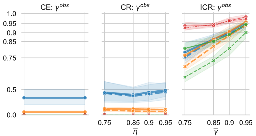
(a) Observed improvement rates $\gamma^{obs}$ (Q1).

(b) causal graphs

method	cost
CE	1.82 $\pm$ 1.09
ind. CR	1.34 $\pm$ 1.14
subp. CR	1.65 $\pm$ 1.02
ind. ICR	4.26 $\pm$ 3.34
subp. ICR	4.20 $\pm$ 3.33

(c) Recourse cost (Q4).

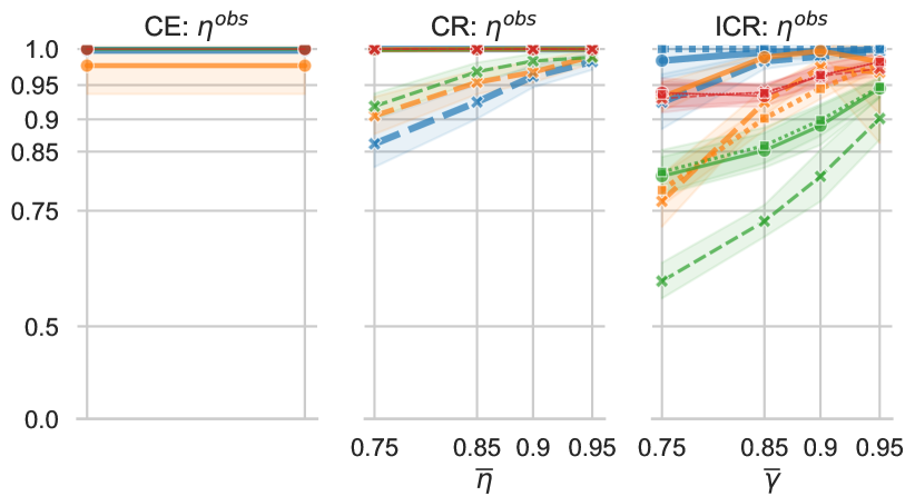
(d) Observed acceptance rates $\eta^{obs}$ w.r.t. $h^{*}$; for ind. ICR additionally w.r.t. $h^{*,ind}$ (Q2).

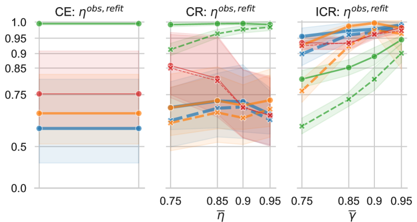
(e) Observed acceptance rates for other fits with comparable test set performance $\eta^{obs,\text{refit}}$ (Q3).

(f) legend

Figure 2: Experimental results for CE, CR and ICR on four datasets over $10$ runs on $200$ individuals each. For the probabilistic methods the confidences $0.75,0.85,0.9,0.95$ were targeted (for CR: $\overline{\eta}$, for ICR: $\overline{\gamma}$). For CE no slack is allowed, such that the results correspond to a confidence level of $1.0$. Values are reported on a quadratic scale.

Q1 (Figure 2a): In scenarios where gaming is possible and lucrative (3var-noncausal, 5var-skill and 7var-covid) ICR reliably guides towards improvement, but CE and CR game the predictor and yield improvement rates close to zero. For instance, on 5var-skill CE and CR exclusively suggest to tune the GitHub profile (e.g. by adding more commits). Since the employer offered recourse it should be honored although the applicants remain unqualified. In contrast, ICR suggests to get a degree or to gain experience, such that recourse implementing individuals are suited for the job.
On 3var-causal, where gaming is not possible, CR also achieves improvement. However, since acceptance w.r.t to a decision treshold $t=0.5$ is targeted, only improvement rates close to $50\%$ are achieved (the expected predicted score translates into $\gamma^{sub}$ (Proposition 3)).
For subp. ICR, $\gamma^{obs}$ is below $\overline{\gamma}$, because the subpopulation may include individuals that were already accepted pre-recourse, such that $\gamma^{sub}$ and $\gamma^{obs}$ may not coincide.

Q2 (Figure 2d): All methods yield the desired acceptance rates w.r.t. to the pre-recourse predictor. For CE and CR $\eta^{obs}$ is higher than for ICR, and for ind. recourse higher than for subp. recourse. Curiously, although no acceptance guarantees could be derived for the pre-recourse predictor and ind. ICR, we find that both pre- and ind. post-recourse predictor reliably lead to acceptance.

Q3 (Figure 2e): We observe that CE and CR actions are unlikely to be honored by other model fits with similar performance on the same data. This result is highly relevant to practitioners, since models deployed in real-world scenarios are regularly refitted. As such, individuals that implemented acceptance-focused recourse may not be accepted after all, since the decision model was refitted in the meantime. In contrast, ICR acceptance rates are nearly unaffected by refits. The result confirms our argument that improvement-focused recourse may be more desirable for explainees (Section 4).

Q4 (Table 2c): CR actions are cheaper than ICR actions, since improvement may require more effort than gaming. As such, CR has benefits for the explainee: For instance, on 5var-skill, CR suggests to tune the GitHub profile (e.g. by adding more commits), which requires less effort than earning a degree or gaining job experience. Detailed results on cost are reported in C.3.

In conclusion, ICR actions require more effort than CR, but lead to improvement and acceptance while being more robust to refits of the model.

9 Limitations and Discussion

Causal knowledge and assumptions

Individualized ICR requires a fully specified SCM; Subpopulation-based ICR is less demanding but still requires the causal graph and causal sufficiency. SCMs and causal graphs are rarely readily available in practice (Peters et al., 2017) and causal sufficiency is difficult to test (Janzing et al., 2012). Research on causal inference gives reason for cautious optimism that the difficulties in constructing SCMs and causal graphs can eventually be overcome (Spirtes and Zhang, 2016; Peters et al., 2017; Heinze-Deml et al., 2018; Malinsky and Danks, 2018; Glymour et al., 2019).
There are further foundational problems linked to causality that affect our approach: causal cycles, an ontologically vague target $Y$ (e.g. in hiring), disparities in our data, or causal model misspecification (Barocas and Selbst, 2016; Barocas et al., 2017; Bongers et al., 2021). All of these factors are considered difficult open problems and may have detrimental impact on our, as well as on any other, recourse framework.
Guiding action without causal knowledge is impossible; when causal knowledge is available, our work provides a normative framework for improvement-focused recourse recommendations. Thus, we join a range of work in explainability (Frye et al., 2020; Heskes et al., 2020; Wang et al., 2021; Zhao and Hastie, 2021) and fairness (Kilbertus et al., 2017; Kusner et al., 2017; Zhang and Bareinboim, 2018; Makhlouf et al., 2020) that highlights the importance of causal knowledge.

Contestability

Improvement-focused recourse guides individuals towards actions that help them to improve, e.g., it recommends a vaccination to lower the risk to get infected with Covid. If, however, a explainee is more interested in contesting the algorithmic decision, (improvement-focused) recourse recommendations are not sufficient. Think of an individual who is denied entrance to an event because of their high Covid risk prediction, which is based on a non-causal, spurious association with their country of origin. In such situations, we suggest to additionally show explainees diverse explanations, which enable to contest the decision. For example, such an explanation could be: if your country of origin would be different, your predicted Covid risk would have been lower.

10 Conclusion

In the present paper, we took a causal perspective and investigated the effect of recourse recommendations on the underlying target variable. We demonstrated that acceptance-focused recourse recommendations like counterfactual explanations or causal recourse may not improve the underlying prediction but game the predictor instead. The problem stems from predictive, but non-causal relationships, which are abundant in machine learning applications.
We tackled the problem in the explanation domain and introduced Improvement-Focused Causal Recourse (ICR), an explanation technique that guides towards improvement of the prediction target and demonstrated how to design post-recourse predictors such that improvement leads to acceptance. We confirm the theoretical results in experiments.
With ICR we hope to inspire a shift from acceptance- to improvement-focused recourse.

Table 1: Overview of important terms and their meanings.

term		meaning
explainee		individual for whom the explanation is generated, e.g. loan applicant
model authority		decision-making entity, e.g. credit institute
recourse		action of the explainee that reverts unfavorable decision
acceptance		desirable model prediction ($\hat{Y}=1$)
improvement		(yield) desirable state of the underlying target ($Y=1$)
gaming		yield acceptance without improvement, e.g. treating the symptoms
pre-/post-recourse		before/after implementing recourse recommendation
contestability		the explainee’s ability to contest an algorithmic decision
robustness of recourse		probability that recourse is accepted despite model/data shifts

Appendix A Extended Background

As follows, we recapitulate well-known definitions in our notation, provide more detailed background on related work and recapitulate results that we use in the proofs. Readers who are already familiar with recourse terminology and $d$-separation (A.1 and A.2), and who are not interested in more detailed introductions of intervention stability (A.3, only required for the proof of Proposition 2) or causal recourse (A.4), may skip this section.

A.1 Overview of important terms

An overview of important terms is provided in Table 1.

A.2 d-separation

Two variable sets $X,Y$ are called $d$-separated [Geiger et al., 1990, Spirtes et al., 2000] by the variable set $Z$ in a graph $\mathcal{G}$ (denoted as $X\perp_{\mathcal{G}}Y|Z$), if, and only if, for every path $p$ it either holds that (i) $p$ contains a chain $i\rightarrow m\rightarrow j$ or a fork $i\leftarrow m\rightarrow j$ where $m\in Z$ or (ii) $p$ contains a collider $i\rightarrow m\leftarrow j$ such that $m$ and for all of its descendants $n$ it holds that $m,n\not\in Z$. Given the causal Markov property, $d$-separation in a causal graph implies (conditional) independence in the data [Peters et al., 2017].

A.3 Generalizability and intervention stability

For Proposition 2, we leverage necessary conditions for invariant conditional distributions as derived in [Pfister et al., 2021]. The authors introduce a $d$-separation based intervention stability criterion that is applied to a modified version of $\mathcal{G}$. For every intervened upon variable $X_{l}$ an auxiliary intervention variable, denoted as $I_{l}$, is added as direct cause of $X_{l}$, yielding $\mathcal{G}^{*}$. The intervention variable can be seen as a switch between different mechanisms. A set $S\subseteq\{1,\dots,d\}$ is called intervention stable regarding a set of actions if for all intervened upon variables $X_{l}$ (where $l\in I^{\text{total}}$) the $d$-separation $I^{l}\perp_{\mathcal{G}^{*}}Y|X_{S}$ holds in $\mathcal{G}^{*}$. The authors show that intervention stability implies an invariant conditional distribution, i.e., for all actions $a,b\in\mathbb{A}$ with $I^{a},I^{b}\subseteq I^{\text{total}}$ it holds that $p(y^{a}|x_{S})=p(y^{b}|x_{S})$ (Pfister et al. [2021], Appendix A).

A.4 Causal recourse

ICR is closely related to the CR framework [Karimi et al., 2020b, 2021], but differs substantially in its motivation and target. In order to allow for a direct comparison we briefly sketch the main ideas and the central CR definitions in our notation. Like ICR, CR aims to guide individuals to revert unfavorable algorithmic decisions (recourse). Therefore, they suggest to search for cost-efficient actions that lead to acceptance by the prediction model. Actions are modeled as structural interventions $a:\Pi\to\Pi$, which can be constructed as $a=do(\{X_{i}:=\theta_{i}\}_{i\in I})$, where $I$ is the index set of features to be intervened upon [Karimi et al., 2021]. The conservativeness of the suggested actions can be adjusted using the hyperparameter $\gamma_{LCB}$, that determines the adaptive threshold $\texttt{thresh}(a)$ and thereby how many standard deviations the expected prediction shall be away from the model’s decision threshold $t$. In order to accommodate different levels of causal knowledge, two probabilistic versions of CR were introduced [Karimi et al., 2020b]: While individualized recourse assumes knowledge of the SCM, subpopulation-based CR only assumes knowledge of the causal graph.

Individualized recourse

Individualized recourse predicts the effect of actions using structural counterfactuals [Karimi et al., 2021], which require a full specification of the SCM.

Given a function that evaluates the cost of actions ($\text{cost}(a,x^{pre})$), the optimization goal for individualized causal recourse is given below. The adaptive threshold thresh bounds the prediction away from the decision threshold.

$$a^{*}\in\underset{a\in\mathbb{A}}{\text{argmin}}\quad\text{cost}(a,x^{pre})\quad \text{s.t. }\mathds{E}[\hat{h}(x^{post})|do(a),x^{pre}]\geq\texttt{thresh}(a)$$

$$\text{with }\texttt{thresh}(a):=0.5+\gamma_{LCB}\sqrt{\text{Var}[\hat{h}(x^{post,a})]}$$

Subpopulation-based recourse:

If no knowledge of the SCM is given, counterfactual distributions cannot be estimated and consequently individualized recourse recommendations cannot be computed. Subpopulation-based CR is based on the average treatment effect within a subgroup of similar individuals [Karimi et al., 2020b]. More specifically individuals belong to the same group if the non-descendants $nd(I)$ of intervention variables (which ceteris paribus remain constant despite the intervention) take the same value. The subpopulation-based objective is given below.

$$a^{*}\in\underset{a\in\mathbb{A}}{\text{argmin}}\text{ cost}(a,x^{pre})\text{ s.t. }\mathds{E}_{X_{d(I)}|do(X_{I}=\theta),x^{pre}_{nd(I)}}[\hat{h}(x^{pre}_{nd(I)},\theta,X_{d(I)})]\geq\texttt{thresh}(a).$$

Appendix B Estimation and Optimization

As follows we provide detailed explanations of the proposed estimation procedures. First, we explain how to sample from the individualized post-recourse distribution, which allows us to estimate the individualized improvement and acceptance rates ($\gamma^{ind}$ and $\eta^{ind}$, B.1). Based on the same sampling mechanism we can also estimate the individualized post-recourse prediction $h^{*,ind}$ (B.2). Then we explain how to sample from the subpopulation-based post-recourse distribution, which allows us to estimate the subpopulation-based improvement and acceptance rates ($\gamma^{sub}$ and $\eta^{sub}$, B.3). Furthermore, we provide details on optimization (B.4) and demonstrate that the optimal observational predictor $h^{*}$ can also be estimated using the SCM (B.5).

B.1 Estimation of the individualized improvement confidence $\gamma^{ind}$ and individualized acceptance rate $\eta^{ind}$

We recall that $\gamma^{ind}$ is the counterfactual probability of the underlying target $Y$ taking the favorable outcome, and $\eta^{ind}$ the counterfactual probability of the prediction $\hat{Y}$ taking the favorable outcome. In order to estimate $\gamma^{ind}$ and $\eta^{ind}$ we first sample covariates and target from the counterfactual post-recourse distribution and then compute the proportion of favorable outcomes for $Y$ and $\hat{Y}$ in the sample.
In general, sampling from counterfactual distributions based on a SCM is performed in three steps (Section 3, [Pearl, 2009]).

1. Abduction: The exogenous noise variables are reconstructed from the observations, i.e., $p(u_{Y,D}|x^{pre})$ is estimated.

2. Intervention: The intervention $do(a)$ on the SCM $\mathcal{M}$ is performed by replacing the respective structural equations $f_{I_{a}}:=\theta_{I_{a}}$, yielding $\mathcal{M}_{do(a)}$.

3. Prediction: The abducted noise variables are sampled from $p(u_{Y,D}|x^{pre})$ and passed through the model $\mathcal{M}_{do(a)}$ to sample from the counterfactual distribution $P(Y^{post},X^{post}|x^{pre},do(a))$.

Given knowledge of the SCM, the challenge is to sample the exogeneous variables from $p(u_{Y,D}|x^{pre})$ (abduction). As follows we explain the abduction in two steps. First, we explain how we can abduct $u_{j}$ for variables for which both the node $x_{j}$ and all parents $(x,y)_{pa(j)}$ are observed, which we refer to as the standard abduction case. Then we factorize the abduction of the joint $p(u_{Y,D}|x^{pre})$ into several components which can be reduced to said standard abduction case. The sampling procedure is summarized in Algorithm 1.

B.1.1 Recap: Standard abduction

If for a node $u_{j}$ both the node $(x,y)_{j}$ and the parents $(x,y)_{p}a(j)$ are observed, we can apply standard abduction. The standard abduction procedure depends on the type of structural equation and exogenous noise distribution.
Given invertible structural equations, observation of $x_{j},x_{pa(j)}$ determines $u_{j}$. More specifically, $u_{j}$ can be reconstructed using

$$u_{j}=f^{-1}(x_{j};x_{pa(j)}).$$

For instance, for additive structural equations $f_{j}(u_{j};x_{pa(j)})=g(x_{pa(j)})+u_{j}$, the inversion is given by $f_{j}^{-1}(x_{j};x_{pa(j)})=x_{j}-g(x_{pa(j)})$.
In our experiments we also included binomial variables with a sigmoidal (non-invertible) structural equation. More specifically, the structural equations are defined as $x_{j}=[\sigma(l(x_{pa(j))})\leq u_{j}]$ with $U_{j}\sim Unif(0,1)$. Here $\sigma$ refers to the sigmoid function and $l$ to some linear combination. $[cond]$ evaluates to $1$ when the condition is true and otherwise to $0$. Intuitively, $\sigma(l(x_{pa(j))})$ can be seen as a nonlinear activation function which determines the probability of the node being activated ($x_{j}=1$). $u_{j}$ acts as a dice, where values $\leq\sigma(l(x_{pa(j))})$ imply $x_{j}=1$ and vice versa.
For those variables, if $x_{j}=1$, we know that $u_{j}\leq\sigma(l(x_{pa(j))})$ and vice versa, such that we can abduct $U_{j}$ as follows (and can therefore sample $u_{j}$):

$$P(U_{j}|x_{j};x_{pa(j)})=\left\{\begin{array}[]{lr}Unif(0,\sigma(l(x_{pa(j)}))),&\text{for }x_{j}=1\\ Unif(\sigma(l(x_{pa(j)})),1),&\text{for }x_{j}=0\end{array}\right.$$

As we will see in the next section, our estimation procedure can be flexibly extended to SCMs with different types of structural equations, as long as a procedure to sample from the abducted exogneous noise variable for the standard case (where parents and the node itself are observed) is available.

B.1.2 Factorization of $p(u|x)$

We have demonstrated how to abduct individual nodes in the standard setting where the corresponding endogenous variable and its parents are observed.
As follows we demonstrate how to sample from the joint distribution of the exogenous variables given an observation of $X$ (and without observing $Y$). Therefore, we show that $p(u|x)$ can be seen as a mixture of two distributions, one for each possible state $y^{\prime}$ of $Y$. In order to sample from it, we (1) need to sample $y^{\prime}$ from the mixing distribution $p(y|x)$ and (2) given $y^{\prime}$, sample from the respective abducted noise variable $p(u|y^{\prime},x)$.

$$p(u|x)\qquad\stackrel{{\scriptstyle\mathclap{\mbox{law tot. prob.}}}}{{=}}\qquad\sum_{y^{\prime}\in\{0,1\}}p(u,y^{\prime}|x)\qquad\stackrel{{\scriptstyle\mathclap{\mbox{cond. prob.}}}}{{=}}\qquad\sum_{y^{\prime}\in\{0,1\}}p(u|y^{\prime},x)p(y^{\prime}|x)$$ (2)

The binomial mixing distribution $p(y|x)$ can be obtained and sampled from by leveraging the cross-entropy optimal predictor $h^{*}$ (which can for instance be derived from the SCM, see B.5). In order to sample from $p(u|y^{\prime},x)$ we leverage the Markov factorization, which allows us to sample each component independently using the standard abduction procedure described above.

$$\begin{split}p(u|x,y^{\prime})\quad\stackrel{{\scriptstyle\mathclap{\mbox{d-sep.}}}}{{=}}\quad&P(u_{Y}|x_{pa(Y)},y^{\prime})\prod_{k\in ch(Y)}P(u_{k}|x_{k},x_{pa(k)},y^{\prime})\prod_{k\not\in ch(Y)}P(u_{k}|x_{k},x_{pa(k)}).\end{split}$$ (3)

The overall procedure is summarized in Algorithm 1.

B.1.3 Estimation of $\gamma^{ind}$ and $\eta^{ind}$

Given the procedure to sample from the individualized post-recourse distribution we can estimate $\gamma^{ind}$ by taking the mean over the samples taken for $Y^{post}$. Similarly, for each sample for $X^{post}$ we can compute the prediction $\hat{y}^{post}$ using either $h\geq t$ or $h^{ind}\geq t$. By taking the mean over all sampled predictions $\hat{y}^{post}$ we can estimate the respective acceptance probability $\eta(t;x^{pre},a,h)$ or $\eta(t;x^{pre},a,h^{ind})$.

Data: pre-recourse observation $x^{pre}$, action $a$ (where $do(a):=do(X_{I_{a}}:=\theta)$), sample size $M$, structural causal model $\mathcal{M}$ with structural equations $f_{j}$, observational predictor $h$

Result: sample from $p(y^{post},x^{post}|x^{pre},do(a))$

get $\mathcal{M}_{do(a)}$ by updating $f_{i}(x_{pa(i)};u_{i}):=\theta_{i}$ for $i\in I_{a}$ ;

for $m\textbf{ in }(0,...,M-1)$ do

       sample $y^{\prime}$ from $Binomial(h(x^{pre}))$ ;

       for $j\textbf{ in }D$ do

             sample $u_{j}^{(m)}$ from $p(u_{j}|(x,y^{\prime})_{j},(x,y^{\prime})_{pa(j)})$ $\triangleright$ comment: leveraging standard abduction;

            

       end for

      sample $u_{Y}^{(m)}$ from $p(u_{Y}|y^{\prime},x_{pa(Y)})$ ;

       compute $(x^{post},y^{post})^{(m)}=f_{\mathcal{M}_{do(a)}}(u^{(m)})$ ;

      

end for

Algorithm 1 Sampling from the individualized post-recourse distribution

B.2 Estimation of the individualized post-recourse prediction

Data: pre-recourse observation $x^{pre}$, action $a$, sample size $M$, structural causal model $\mathcal{M}$, observational predictor $h$, $m=0$

Result: $\hat{h}^{ind}(x^{post};x^{pre},do(a))$

while $m<M$ do

       sample $(x^{\prime},y^{\prime})$ using Alg. 1 and $x^{pre},a,\mathcal{M},h$;

       if $x^{\prime}=x^{post}$ then

             $m=m+1$; store $y^{\prime}$ as $y^{\prime(m)}$ ;

            

       end if

      

end while

$\hat{h}^{ind}(x^{post})=\frac{1}{M}\sum_{m=1}^{M}y^{\prime(m)}$

Algorithm 2 Estimating $h^{*,ind}$

We continue to show how the individualized post-recourse prediction can be estimated. We recall that $h^{*,ind}$ is

$$h^{*,ind}(x^{post};x^{pre},a)=P(Y^{post}=1|x^{post},x^{pre},do(a)).$$

We can estimate $h^{*,ind}$ by leveraging the procedure to sample from the post-recourse covariate distribution (Algorithm 1). More specifically, we draw samples $(y^{\prime},x^{\prime})$ from $P(Y^{post},X^{post}|do(a),x^{pre})$ and keep those that conform with $x^{post}$ (i.e., $x^{\prime}=x^{post}$). Within the subsample, we compute the proportion of samples for which $y^{\prime}=1$ to estimate $p(y^{post}|x^{pre},x^{post},do(a))$. In more formal terms, we approximate Eq. 4 using rejection sampling and Monte Carlo integration [Koller and Friedman, 2009].
If the structural equations are invertible or the nodes are categorical the procedure is tractable, since many or all samples conform with $x^{post}$. Otherwise the estimation may become intractable. We see the application of likelihood weighting or MCMC as promising directions and refer interested readers to Koller and Friedman [2009].
In addition to the sampling-based procedure we also derive a closed-form solution for settings with invertible structural equations, which is provided in Proposition 5, Eq. 5.

Proposition 5.

In general, the individualized post-recourse predictor can be estimated as

$$\begin{split}&p(y^{post}|x^{pre},x^{post},do(a))\\ &=\frac{\int_{\mathcal{U}}p(y^{post},x^{post}|u,do(a))p(u|x^{pre})du}{\sum_{y^{\prime}\in\{0,1\}}\left(\int_{\mathcal{U}}p(y^{\prime},x^{post}|u,do(a))p(u|x^{pre})du\right)}\end{split}$$ (4)

Given invertible structural equations, the individualized post-recourse prediction function reduces to

$$\begin{split}&p(y^{post}|x^{post},x^{pre},do(a))\\ &=\frac{p(U_{-I}=f_{do(a)}^{-1}(y^{post},x^{post})|x^{pre},do(a))}{\sum_{y^{\prime}\in\{0,1\}}p(U_{-I}=f_{do(a)}^{-1}(y^{\prime},x^{post})|x^{pre},do(a))}.\end{split}$$ (5)

B.3 Estimation of the subpopulation-based improvement confidence $\gamma^{sub}$ and the subpopulation-based acceptance rate $\eta^{sub}$

As follows we detail how to estimate $\gamma^{sub}$ and $\eta^{sub}$. We focus on actions $a$ that potentially affect $Y$, meaning that they intervene on causes of $Y$.
In order to estimate $\gamma^{sub}$ and $\eta^{sub}$ we sample $(x^{\prime},y^{\prime})$ from the subpopulation-based post-recourse distribution. Given a sample from the subpopulation-based post-recourse distribution we can estimate $\gamma^{sub}$ and $\eta^{sub}$ by taking the respective sample means.
We explain the sampling procedure in two steps: We first recall how causal graphs can be leveraged to sample interventional distributions, and then explain why we can apply the procedure to sample from the subpopulation-based post-recourse distribution.

Recap: Sampling interventional distributions leveraging a causally sufficient causal graph $\mathcal{G}$

Given a causal graph $\mathcal{G}$ (that fulfills the global Markov property), the joint distribution $P(X,Y)$ can be reformulated using the Markov factorization, which makes use of the $d$-separations in the graph.

$$p(x,y)=p(y|x_{pa(y)})\prod_{j\in D}p(x_{j}|(x,y)_{pa(j)})$$

As a consequence, we can sample from the joint distribution by sampling each component given its respective parents. In order to ensure that the parents for each node have been sampled already, the graph is traversed in topological order, starting with the root node and ending with the sink nodes [Koller and Friedman, 2009].
Given that causal sufficiency (no unobserved confounders) and the principle of independent mechanisms hold, the same procedure can also be applied when sampling from interventional distributions of the form $p(x,y|do(a))$ by leveraging the so-called truncated factorization. The intervened upon nodes are not sampled from their parents, but fixed to the values $\theta_{a}$. The remaining nodes $\Gamma$ are sampled as before:

$$\begin{split}&p((x,y)_{\Gamma}|do(a))=\prod_{j\in\Gamma}p((x,y)_{j}|(x,y)_{pa(j)\cap\Gamma},\theta_{pa(j)\cap I_{a}})\\ &\text{with}\quad\Gamma:=D\backslash I_{a}\end{split}$$

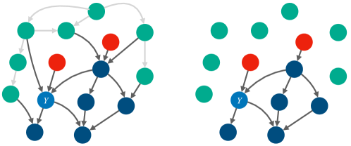
Figure 3: Causal graph $\mathcal{G}_{\overline{I_{a}}}$ visualizing the subpopulation-based post-recourse setting, including the prediction target $Y$ (light blue), intervened-upon variables $I_{a}$ (red), the subgroup characteristics $G_{a}$ (cyan) and the descendants $\Gamma$ that shall be resampled (dark blue). $\overline{I_{a}}$ indicates that incoming edges to $I_{a}$ were removed. Right: Causal graph $\mathcal{G}_{\overline{I_{a}}\underline{G_{a}}}$ where incoming edges to $I_{a}$ and outgoing edges from $G_{a}$ were removed. We observe that in this manipulated graph $G_{a}$ is $d$-separated from $\Gamma$. Thus, according to the second rule of $do$-calculus, for $G_{a}$ intervention and conditioning coincide.

Sampling from the subpopulation-based post-recourse distribution using $\mathcal{G}$

We recall that for actions $a$ that potentially affect $Y$ the subpopulation-based post-recourse distribution is defined as

$$P(Y^{post},X^{post}|do(a),X^{post}_{G_{a}}=x^{pre}_{G_{a}}).$$ (6)

As we will see, the previously described sampling procedure can be applied. Therefore we apply the second rule of $do$-calculus to show that in Equation 6 conditioning on $x_{G_{a}}$ is equal to intervening $do(X_{G_{a}}=x_{G_{a}})$. More specifically, if we remove all outgoing edges from $X_{G_{a}}$ and all incoming edges to $I_{a}$, then $X_{G_{a}}$ and $X_{\Gamma}$ with $\Gamma:=D\backslash I_{a}\cap G_{a}=d(I_{a})$ are $d$-separated, meaning that conditioning and intervention are equivalent (Figure 3).

$$P((Y,X)^{post}_{\Gamma}|do(a),X^{post}_{G_{a}}=x^{pre}_{G_{a}})$$

$$=P((Y,X)^{post}_{\Gamma}|do(a),do(X^{post}_{G_{a}}=x^{pre}_{G_{a}}))$$

As follows we can leverage the procedure to sample interventional distributions to sample from the subpopulation-based post-recourse distribution. The procedure is illustrated in Algorithm 3.

Data: pre-recourse observation $x^{pre}$, action $a$ with $I_{a}\cap asc(Y)\neq\emptyset$ ($do(a):=do(X_{I_{a}}:=\theta)$), sample size $M$, causal graph $\mathcal{G}$, conditional distributions $P(X_{j}|X_{pa(j)})$ for $j\in\Gamma$ with $\Gamma:=\{r:r\in asc(Y)\wedge r\in d(I)\}$

Result: sample from $p(y,x_{\Gamma}|do(a),x_{G_{a}})$

for $m\leftarrow 0$ to $M$ do

       $\Gamma^{sorted}\leftarrow\text{topologicalsort}(\;\Gamma;\mathcal{G}_{do(a)})$ $\triangleright$ sort such that causes precede effects ;

       for $j\textbf{ in }\Gamma^{sorted}$ do

             sample $(x,y)_{j}^{post,(m)}$ $\sim P((X,Y)_{j}|(X,Y)_{pa(j)}=(x,y)_{pa(j)}^{post})$ ;

            

       end for

      

end for

Algorithm 3 Sampling from the subpopulation-based post-recourse distribution

B.3.1 Learning the conditional distributions $P(X_{j}|x_{pa(j)})$

In this work we assume that we have prior knowledge that allows us to sample from the components of the factorization ($P(X_{j}|x_{pa(j)})$, e.g. available if we know the SCM).
If the conditional distributions are not known, they can be learned from observational data; depending on which assumptions about distribution and functional can be made, different techniques may be employed. For categorical variables the problem reduces to standard supervised learning with cross-entropy loss. For linear Gaussian data, the conditional distribution can be estimated analytically from the covariance matrix [Page Jr, 1984]. A variety of estimation techniques exist for continuous settings with nonlinearities [Bishop, 1994, Bashtannyk and Hyndman, 2001, Sohn et al., 2015, Trippe and Turner, 2018, Winkler et al., 2019, Hothorn and Zeileis, 2021].

B.4 Optimization

Like the optimization problems for CE [Wachter et al., 2017, Tsirtsis and Gomez Rodriguez, 2020] or CR [Karimi et al., 2020b], the optimization problem for ICR is computationally challenging. It can be seen as a two-stage problem, where in the first stage the intervention targets $I_{a}$, and in the second stage the corresponding intervention values $\theta_{a}$ are optimized [Karimi et al., 2020b]. For the selection of intervention targets $I_{a}$ alone $2^{d^{\prime}}$ combinations exist, with $d^{\prime}\leq d$ being the number of causes of $Y$. We jointly optimize the intervention targets and the intervention values using a genetic algorithm called NSGA-II [Deb et al., 2002]. For mixed categorical and continuous data, previous work in the field [Dandl et al., 2020] suggests to use NSGA-II in combination with mixed integer evaluation strategies [Li et al., 2013]. The exact hyperparameter configurations are reported in C.3.

B.5 Estimation of the optimal observational predictor $h^{*}$ using the SCM

Instead of leveraging supervised learning with cross-entropy loss, we can factorize the optimal observational predictor as shown in Proposition 6 and then leverage the SCM for the estimation.

Proposition 6.

The optimal observational predictor can be factorized into conditional distributions of nodes given their parents (using the Markov factorization). More specifically, we yield

$$p(y|x)=\frac{p(x,y)}{p(x)}=\frac{p(x,y)}{\sum_{y^{\prime}\in\{0,1\}}p(x,y)}$$ (7)

$$\quad\stackrel{{\scriptstyle\mathclap{\mbox{M.f.}}}}{{=}}\frac{p(y|x_{pa(j)})\prod_{j\in D}p(x_{j}|(x,y)_{pa(j)})}{\sum_{y^{\prime}\in\{0,1\}}p(y^{\prime}|x_{pa(j)})\prod_{j\in D}p(x_{j}|(x,y^{\prime})_{pa(j)})}$$ (8)

$$\quad=\frac{p(y|x_{pa(j)})\prod_{j\in ch(y)}p(x_{j}|x_{pa(j)},y)}{\sum_{y^{\prime}\in\{0,1\}}p(y^{\prime}|x_{pa(j)})\prod_{j\in ch(y)}p(x_{j}|x_{pa(j)},y^{\prime})}.$$ (9)

It remains to show how the conditional distribution $p(x_{j}|x_{pa(j)})$ of a node given its parents can be estimated. Generally it holds that

$$p(x_{j}|x_{pa(j)})$$ (10)

$$\qquad\stackrel{{\scriptstyle\mathclap{\mbox{law tot. prob.}}}}{{=}}\qquad\int_{\mathcal{U}_{j}}p(x_{j}|x_{pa(j)},u_{j})p(u_{j}|x_{pa(j)})du$$ (11)

$$\qquad\stackrel{{\scriptstyle\mathclap{\mbox{SCM, $u_{j}\perp x_{pa(j)}$}}}}{{=}}\quad\qquad\int_{\mathcal{U}_{j}}[f(x_{pa(j)},u_{j})=x_{j}]p(u_{j})du.$$ (12)

The integral can be approximated using Monte Carlo integration: we can sample from $p(u_{j})$, compute the respective $\tilde{x}_{j}=f_{j}(x_{pa(j)},\tilde{u}_{j})$ and compute the proportion of cases where $x_{j}=\tilde{x}_{j}$. If $X_{j}$ and $U_{j}$ are continuous, this may require huge sample sizes to converge.
Furthermore, we may be able to leverage assumptions about $f_{j}$ to derive a closed form solution. If $f_{j}$ is invertible, the integral reduces to $p(x_{j}|x_{pa(j)})=p(U_{j}=f_{j}^{-1}(x_{j},x_{pa(j)}))$. For binary nodes with $x_{j}:=[\sigma(l(x_{pa(j)}))\leq u_{j}]$ and $U_{j}\sim Unif(0,1)$, we directly see that $p(x_{j}|x_{pa(j)})=\sigma(l(x_{pa(j)}))$.

Appendix C Details on Experiments

In this section we provide additional details on the experiments. More specifically, we explain which open-source libraries we use, how to access our code and how to reproduce the results in C.1. We formally introduce the synthetic and semi-synthetic datasets that we used in our experiments in C.2 and the corresponding figures. Details on hyperparameters, models as well as detailed results are reported in C.3 and the corresponding tables.

C.1 Implementation

The code relies of efficient tensor calculations with numpy [Harris et al., 2020], pytorch [Paszke et al., 2019] and jax [Bradbury et al., 2018]. For named dataframes we use pandas [pandas development team, 2020]. For plotting we rely on matplotlib [Hunter, 2007] and seaborn [Waskom, 2021]. We use the evolutionary optimization library deap [Fortin et al., 2012] and NSGA-II [Deb et al., 2002] to solve the combinatorial optimization problem. In order to speed up the computation, we cache queries and results for the improvement confidence using functools.cache. For continuous variables the intervention can be rounded to a specified number of digits to increase the probability of reusing a cached result (with neglectable loss of precision).

All code is publicly available via https://github.com/gcskoenig/icr. The repository contains the user-friendly python package icr, which we use in our experiments to generate and evaluate recourse. Furthermore, the scripts for the experiments, the scripts for the visualization of the results as well as a README.md with instructions for the installation of all dependencies are contained in the repository, such that the experiments are reproducible.

C.2 Synthetic and Semi-Synthetic Datasets

3var-causal and 3var-noncausal are abstract, synthetic settings. 5var-skill is inspired by Montandon et al. [2021], who use GitHub profiles to detect the role of a developer. In our SCM we model senior-level skill as a binary variable which is caused by programming experience and the education degree. The skill is causal for GitHub metrics such as the number of commits, the number of programming languages and the number of stars. The 7var-covid dataset is inspired by Jehi et al. [2020]. The following variables are introduced: population density $D$, flu vaccination $V_{I}$, number of covid vaccination shots $V_{C}$, deviation from average BMI $B$, whether someone is free of covid disease $C$, whether the individual has influence $I$, appetite loss $S_{A}$, fever $S_{Fe}$ and fatigue $S_{Fa}$. The corresponding structural equations, noise distributions and causal graphs are provided in Figure 4 (3var-causal), 5 (3var-noncausal), 6 (5var-skill) and 7 (7var-covid). A pairplot for each dataset is presented in Figure 8. In our notation $\sigma$ is the sigmoid function, $N$ the Gaussian distribution, $Cat$ a categorical distribution, $Unif$ the uniform distribution, $Bern$ a Bernoulli distribution and $GaP$ a Gamma-Poisson mixture. $\left[cond\right]$ is $1$ when the condition is met and $0$ if not. As a consequence variables with $\left[Z\leq U\right]$ and $U\sim Unif(0,1)$ are bernoulli distributed with $Bern(Z)$.

(a) Causal graph

$$X_{1} :=U_{1}, U_{1}\sim N(0,1)$$

$$X_{2} :=X_{1}+U_{2}, U_{2}\sim N(0,1)$$

$$X_{3} :=X_{1}+X_{2}+U_{3}, U_{3}\sim N(0,1)$$

$$Y \sim\left[\sigma(X_{1}+X_{2}+X_{3})\leq U_{Y}\right], U_{Y}\sim Unif(0,1)$$

(b) Structural Equations

Figure 4: SCM for 3var-causal. The cost function is given as $cost(a)=\delta_{1}+\delta_{2}+\delta_{3}$, where $\delta$ is the vector of absolute changes to the intervened upon variables. E.g., for $do(a)=do(X_{1}=x_{1}^{\prime})$, $\delta_{1}=|x_{1}^{\prime}-x_{1}|$ and $\delta_{2}=\delta_{3}=0$

(a) Causal graph

$$X_{1} :=U_{1}, U_{1}\sim N(0,1)$$

$$X_{2} :=X_{1}+U_{1}, U_{1}\sim N(0,1)$$

$$Y :=\left[\sigma(X_{1}+X_{2})\leq U_{Y}\right], U_{Y}\sim Unif(0,1)$$

$$X_{3} :=X_{1}+X_{2}+Y+U_{3}, U_{3}\sim N(0,0.1)$$

(b) Structural Equations

Figure 5: SCM for 3var-noncausal with $cost(a)=\delta_{1}+\delta_{2}+\delta_{3}$.

(a) Causal graph

$$E :=U_{E};U_{E}\sim GaP(8,8/3)$$

$$D :=U_{D};U_{D}\sim Cat(0.4,0.2,0.3,0.1)$$

$$S :=\left[\sigma(-10+3E+4D))\leq U_{S}\right];U_{S}\sim Unif(0,1)$$

$$G_{C} :=10E(11+100D)+U_{G_{C}};U_{G_{C}}\sim GaP(40,40/4)$$

$$G_{L} :=\sigma(10S)+U_{G_{L}};U_{G_{L}}\sim GaP(2,2/4)$$

$$G_{S} :=10S+U_{G_{S}};U_{G_{S}}\sim GaP(5,5/4)$$

(b) Structural Equations

Figure 6: SCM for 5var-skill with $cost(a)=5\delta_{E}+5\delta_{D}+0.0001\delta_{G_{C}}+0.01\delta_{G_{L}}+0.1\delta{G_{S}}$.

(a) Causal graph

$$D :=U_{D};U_{D}\sim\Gamma(4,4/3)$$

$$V_{I} :=U_{V_{I}};U_{V_{I}}\sim Bern(0.39)$$

$$V_{C} :=U_{V_{C}};U_{V_{C}}\sim Cat(0.24,0.02,0.15,0.59)$$

$$B :=U_{B};U_{B}\sim N(0,1)$$

$$C :=\left[\sigma(-(D-3-V_{I}-2.5V_{C}+0.2B^{2}))\leq U_{C}\right];$$

$$U_{C} \sim Unif(0,1)$$

$$S_{A} :=\left[\sigma(-2C)\leq U_{S_{A}}\right];U_{S_{A}}\sim Unif(0,1)$$

$$S_{Fe} :=\left[\sigma(5-9C)\leq U_{S_{Fe}}\right];U_{S_{Fe}}\sim Unif(0,1)$$

$$S_{Fa} :=\left[\sigma(-1+B^{2}-2C)\leq U_{S_{Fa}}\right];$$

$$U_{S_{Fa}} \sim Unif(0,1)$$

(b) Structural Equations

Figure 7: SCM for 7var-covid with cost function $cost(a)=\delta_{D}+\delta_{V_{I}}+\delta_{V_{C}}+\delta_{B}+\delta_{S_{A}}+\delta_{S_{Fe}}+\delta_{S_{Fa}}$.

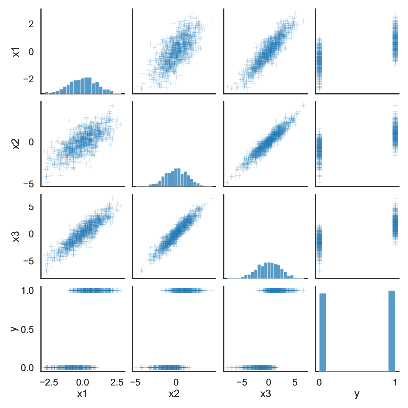
(a) Pairplot for 3var-causal.

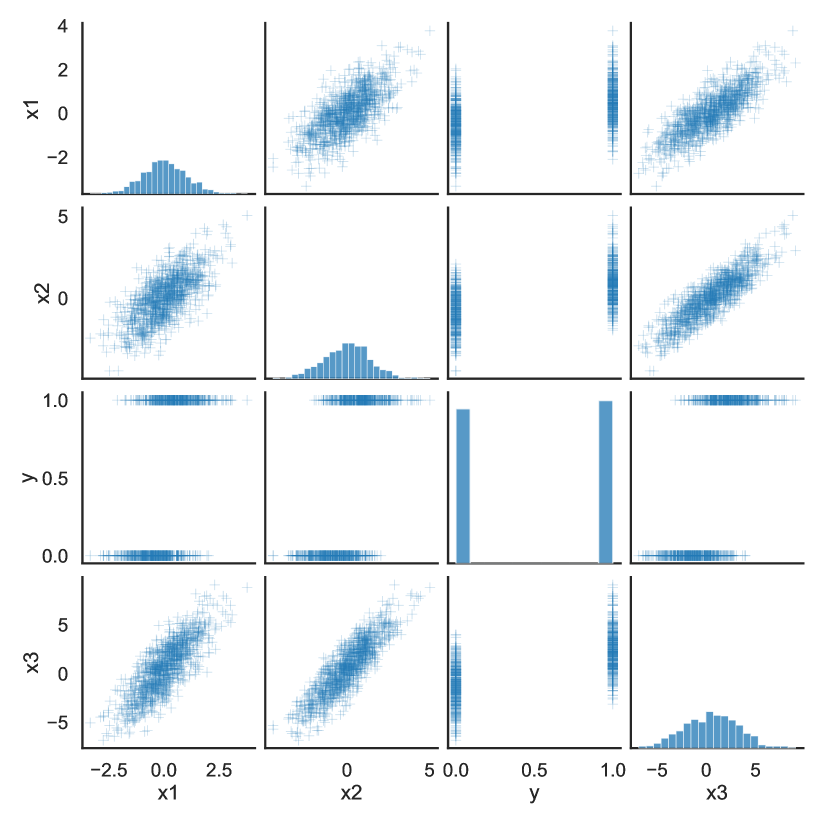
(b) Pairplot for 3var-noncausal.

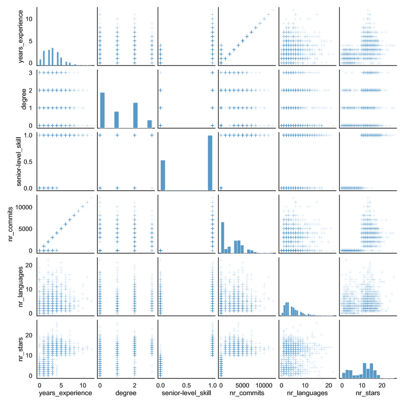
(c) Pairplot for 5var-skill.

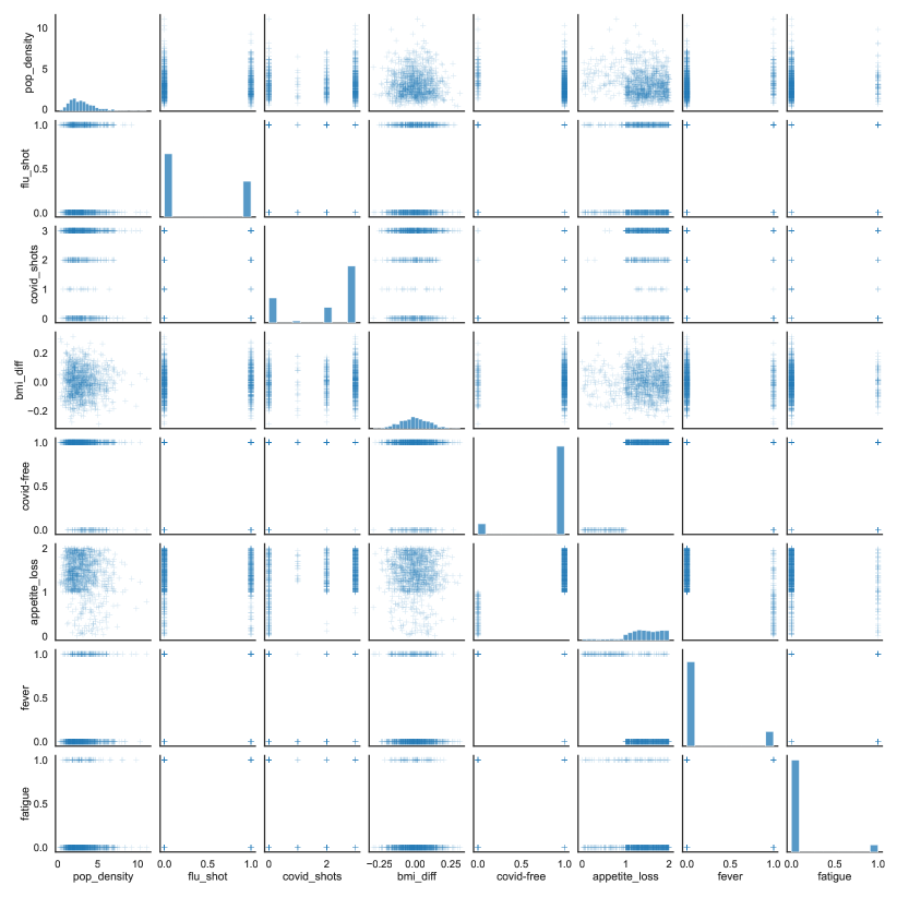
(d) Pairplot for 7var-covid.

Figure 8: Pairplots for the SCMs.

C.3 Detailed Results

Table 2: Results for 3var-causal.

3var-causal	$\overline{\gamma}$ / $\overline{\eta}$	$\gamma_{\text{obs.}}$	$\pm$	$\eta_{\text{obs.}}$	$\pm$	$\eta^{individ.}_{\text{obs.}}$	$\pm$	$\eta^{\text{refit}}_{\text{obs.}}$	$\pm$	$\emptyset$ cost	$\pm$
CE	-	0.41	0.09	1.00	0.00	-	-	0.60	0.20	3.08	0.41
ind. CR	0.75	0.47	0.10	1.00	0.00	-	-	0.70	0.10	2.46	0.37
ind. CR	0.85	0.44	0.08	1.00	0.00	-	-	0.72	0.12	2.39	0.25
ind. CR	0.90	0.47	0.09	1.00	0.00	-	-	0.72	0.14	2.36	0.35
ind. CR	0.95	0.49	0.07	1.00	0.00	-	-	0.67	0.10	2.44	0.31
subp. CR	0.75	0.46	0.11	0.86	0.04	-	-	0.64	0.14	2.66	0.41
subp. CR	0.85	0.43	0.08	0.93	0.02	-	-	0.69	0.14	2.64	0.32
subp. CR	0.90	0.45	0.09	0.96	0.02	-	-	0.70	0.15	2.73	0.42
subp. CR	0.95	0.48	0.09	0.98	0.01	-	-	0.64	0.14	2.86	0.41
ind. ICR	0.75	0.79	0.06	0.98	0.02	1.0	0.0	0.96	0.03	3.27	0.50
ind. ICR	0.85	0.86	0.03	1.00	0.01	1.0	0.0	0.97	0.02	3.82	0.30
ind. ICR	0.90	0.90	0.02	1.00	0.01	1.0	0.0	0.98	0.03	3.70	0.31
ind. ICR	0.95	0.95	0.01	1.00	0.00	1.0	0.0	0.99	0.01	4.08	0.24
subp. ICR	0.75	0.75	0.04	0.93	0.04	-	-	0.90	0.04	3.34	0.49
subp. ICR	0.85	0.87	0.03	0.98	0.01	-	-	0.96	0.02	4.05	0.29
subp. ICR	0.90	0.89	0.02	0.99	0.01	-	-	0.97	0.02	3.87	0.25
subp. ICR	0.95	0.94	0.02	1.00	0.00	-	-	0.99	0.01	4.22	0.28

Table 3: Results for 3var-noncausal

3var-noncausal	$\overline{\gamma}$ / $\overline{\eta}$	$\gamma_{\text{obs.}}$	$\pm$	$\eta_{\text{obs.}}$	$\pm$	$\eta^{individ.}_{\text{obs.}}$	$\pm$	$\eta^{\text{refit}}_{\text{obs.}}$	$\pm$	$\emptyset$ cost	$\pm$
CE	-	0.17	0.03	0.98	0.04	-	-	0.67	0.15	2.28	0.26
ind. CR	0.75	0.25	0.03	1.00	0.00	-	-	0.70	0.13	2.28	0.21
ind. CR	0.85	0.24	0.02	1.00	0.00	-	-	0.73	0.13	2.29	0.17
ind. CR	0.90	0.24	0.04	1.00	0.00	-	-	0.71	0.11	2.24	0.16
ind. CR	0.95	0.23	0.04	1.00	0.00	-	-	0.73	0.12	2.18	0.32
subp. CR	0.75	0.22	0.03	0.91	0.03	-	-	0.63	0.15	2.18	0.12
subp. CR	0.85	0.19	0.03	0.95	0.02	-	-	0.67	0.15	2.33	0.21
subp. CR	0.90	0.19	0.03	0.97	0.01	-	-	0.65	0.14	2.42	0.19
subp. CR	0.95	0.19	0.03	0.99	0.01	-	-	0.69	0.14	2.26	0.32
ind. ICR	0.75	0.77	0.03	0.93	0.02	0.79	0.03	0.93	0.02	2.16	0.11
ind. ICR	0.85	0.86	0.02	0.99	0.01	0.90	0.02	0.99	0.01	2.51	0.08
ind. ICR	0.90	0.91	0.03	1.00	0.00	0.94	0.01	1.00	0.00	3.00	0.08
ind. ICR	0.95	0.96	0.02	0.98	0.07	0.98	0.01	0.98	0.08	3.32	0.16
subp. ICR	0.75	0.69	0.03	0.77	0.05	-	-	0.76	0.05	2.11	0.20
subp. ICR	0.85	0.82	0.03	0.93	0.02	-	-	0.92	0.02	2.42	0.11
subp. ICR	0.90	0.89	0.03	0.98	0.01	-	-	0.97	0.01	2.86	0.13
subp. ICR	0.95	0.94	0.02	0.97	0.10	-	-	0.96	0.12	3.19	0.15

Table 4: Results for 5var-skill

5var-skill	$\overline{\gamma}$ / $\overline{\eta}$	$\gamma_{\text{obs.}}$	$\pm$	$\eta_{\text{obs.}}$	$\pm$	$\eta^{individ.}_{\text{obs.}}$	$\pm$	$\eta^{\text{refit}}_{\text{obs.}}$	$\pm$	$\emptyset$ cost	$\pm$
CE	-	0.00	0.00	1.00	0.00	-	-	0.76	0.14	1.34	1.28
ind. CR	0.75	0.00	0.00	1.00	0.00	-	-	0.86	0.11	0.27	0.28
ind. CR	0.85	0.00	0.00	1.00	0.00	-	-	0.81	0.14	0.24	0.20
ind. CR	0.90	0.00	0.01	1.00	0.00	-	-	0.70	0.15	0.10	0.00
ind. CR	0.95	0.00	0.00	1.00	0.00	-	-	0.66	0.16	0.11	0.03
subp. CR	0.75	0.00	0.00	1.00	0.00	-	-	0.85	0.11	4.06	4.97
subp. CR	0.85	0.00	0.00	1.00	0.00	-	-	0.80	0.15	0.24	0.19
subp. CR	0.90	0.00	0.01	1.00	0.00	-	-	0.70	0.15	0.10	0.01
subp. CR	0.95	0.00	0.00	1.00	0.00	-	-	0.66	0.15	0.12	0.04
ind. ICR	0.75	0.94	0.02	0.94	0.02	0.94	0.02	0.94	0.02	4.95	5.32
ind. ICR	0.85	0.94	0.01	0.93	0.02	0.94	0.01	0.93	0.02	9.80	0.27
ind. ICR	0.90	0.96	0.02	0.96	0.02	0.96	0.02	0.96	0.02	10.38	0.23
ind. ICR	0.95	0.98	0.01	0.98	0.01	0.98	0.01	0.98	0.01	11.23	0.21
subp. ICR	0.75	0.93	0.01	0.93	0.02	-	-	0.93	0.01	4.72	5.08
subp. ICR	0.85	0.94	0.01	0.94	0.01	-	-	0.94	0.02	9.74	0.17
subp. ICR	0.90	0.96	0.01	0.96	0.01	-	-	0.96	0.01	10.46	0.53
subp. ICR	0.95	0.97	0.01	0.97	0.01	-	-	0.97	0.01	10.88	0.21

Table 5: Results for 7var-covid

7var-covid	$\overline{\gamma}$ / $\overline{\eta}$	$\gamma_{\text{obs.}}$	$\pm$	$\eta_{\text{obs.}}$	$\pm$	$\eta^{individ.}_{\text{obs.}}$	$\pm$	$\eta^{\text{refit}}_{\text{obs.}}$	$\pm$	$\emptyset$ cost	$\pm$
CE	-	0.00	0.00	1.00	0.00	-	-	1.00	0.00	0.60	0.12
ind. CR	0.75	0.01	0.00	1.00	0.00	-	-	0.99	0.01	0.56	0.02
ind. CR	0.85	0.00	0.00	1.00	0.00	-	-	0.99	0.00	0.55	0.02
ind. CR	0.90	0.00	0.00	1.00	0.00	-	-	1.00	0.00	0.55	0.03
ind. CR	0.95	0.00	0.00	1.00	0.00	-	-	0.99	0.01	0.54	0.07
subp. CR	0.75	0.01	0.01	0.92	0.02	-	-	0.91	0.02	0.52	0.03
subp. CR	0.85	0.00	0.01	0.97	0.01	-	-	0.96	0.01	0.75	0.40
subp. CR	0.90	0.00	0.00	0.98	0.01	-	-	0.98	0.01	0.55	0.03
subp. CR	0.95	0.00	0.00	0.99	0.01	-	-	0.98	0.01	0.51	0.07
ind. ICR	0.75	0.81	0.03	0.81	0.03	0.82	0.04	0.81	0.03	1.26	0.02
ind. ICR	0.85	0.85	0.03	0.85	0.03	0.86	0.03	0.85	0.03	1.14	0.44
ind. ICR	0.90	0.89	0.03	0.89	0.03	0.90	0.02	0.89	0.03	1.61	0.02
ind. ICR	0.95	0.95	0.01	0.95	0.01	0.95	0.01	0.95	0.01	1.97	0.06
subp. ICR	0.75	0.61	0.04	0.61	0.04	-	-	0.61	0.04	1.06	0.03
subp. ICR	0.85	0.73	0.03	0.73	0.03	-	-	0.73	0.03	1.09	0.34
subp. ICR	0.90	0.81	0.04	0.81	0.04	-	-	0.81	0.04	1.42	0.05
subp. ICR	0.95	0.90	0.03	0.90	0.03	-	-	0.90	0.03	1.73	0.06

In this section we report all experimental results in tabular form. More specifically, the results for 3var-causal are reported in Table 2, for 3var-noncausal in Table 3, for 5var-skill in Table 4 and for 7var-covid in Table 5. For each experiment we report the specified confidence $\gamma$ (or $\eta$ for CR), as well as the observed improvement rate $\gamma_{obs}$, the observed acceptance rate $\eta_{obs}$, the observed acceptance rate by the individualized post-recourse predictor $\eta_{obs}^{\text{indiv.}}$, the observed acceptance rate on refits $\eta_{obs}^{\text{refit}}$ and the average recourse cost for individuals who were rejected and whom were provided with a recourse recommendation. A visual summary of the results is provided in Section 8.

In order to enable a more direct comparison of the CR and ICR targets, we equalize the optimization thresholds for ICR and CR. More specifically, for CR we require the (individualized or subpopulation-based) acceptance probability to be $\geq\eta$, and for ICR we require the (individualized or subpopulation-based) improvement probability to be $\geq\overline{\gamma}$, where $\overline{\gamma}=\overline{\eta}$. Furthermore, in order to be able to estimate the effects of recourse actions, CR assumes causal sufficiency, meaning that there are no two endogeneous variables that share an unobserved cause. If the target variable $Y$ is exogeneous then any causal model with more than one endogeneous direct effect of $Y$ violates the assumptions. In order to enable an application of CR on datasets with more than one effect variable we assume knowledge of the SCM including $Y$ for CR as well and draw ground-truth interventional samples from the SCM instead of identifying the interventional distribution from observational data.

For 3var-causal and 3var-noncausal we configured NSGA-II to optimize over $600$ generations with a population size of $300$, for 5var-skill and 7var-covid $1000$ generations with $500$ individuals were used. For all experiments the crossover probability was $0.3$ and the mutation probability $0.05$. For all settings continuous variables were rounded to $1$ decimal point. For the 3 variable settings a standard sklearn LogisticRegression was used, for the refits without penality. For the nonlinear dataset a RandomForestClassifier with max depth $30$, $50$ estimators and balanced subsampling was applied. The experimental results were computed on a Quad core Intel Core i7-7700 Kaby Lake processor. For each setting, the experiments took between 24 to 48 hours.

Appendix D Proofs

As follows we provide the full proofs for Propositions 1 - 5.

D.1 Linking individualized prediction with $\gamma^{ind}$, Proof of Proposition 1

Proposition 1.

The expected individualized post-recourse score is equal to the individualized improvement probability $\gamma^{ind}(x^{pre},a):=P(Y^{post}=1|x^{pre},do(a))$, i.e.

$$E[\hat{h}^{*,ind}(x^{post})|x^{pre},do(a)]=\gamma^{ind}(a).$$

Proof: It holds that

$$E[h^{*,ind}(x^{post})|x^{pre},do(a)]$$

$$=E[E[Y|x^{pre},x^{post}]|x^{pre},do(a)]$$

$$\stackrel{{\scriptstyle\mathclap{\mbox{total exp.}}}}{{=}}\qquad E[Y|x^{pre},do(a)]$$

$$=\gamma^{ind}(a).$$

D.2 Intervention stability w.r.t. ICR actions, Proposition 2

Proposition 2.

Given nonzero cost for all interventions, ICR exclusively suggests actions on causes of $Y$. Assuming causal sufficiency, for any optimal predictor the conditional distribution of $Y$ given the variables that the model uses $X_{S}$ (i.e. $P(Y|X_{S})$) is stable w.r.t interventions on causes. Therefore, optimal predictors are intervention stable w.r.t. ICR actions.

Proof: We prove the statement in six steps.

ICR only intervenes on causes: The goal of meaningful recourse is to improve $Y$ with minimal cost. Only interventions on causes alter $Y$. Consequently, actions on non-causes of $Y$ would not be suggested by meaningful recourse.

Given causal sufficiency, a graph $\mathcal{G}$ and an endogenous $Y$, the set of endogeneous direct parents, direct effects and direct parents of effects are the minimal $d$-separating set $S_{\mathcal{G}}$: Standard result, see e.g. Peters et al. [2017], Proposition 6.27.

The set $S_{\mathcal{G}^{*}}$ in the augmented graph $\mathcal{G}^{*}$ coincides with $S_{\mathcal{G}}$: The minimal $d$-separating set contains direct causes, direct effects and direct parents of direct effects. $I_{l}$ is never a direct cause of $X_{l}$. Also, since $I_{l}$ has no endogenous causes, it cannot be a direct effect. Furthermore, since we restrict interventions to be performed on causes, $I_{l}$ cannot be a direct parent of a direct effect.

$S_{\mathcal{G}}$ is intervention stable: As follows, all intervention variables are $d$-separated from $Y$ in $\mathcal{G^{*}}$ by $S_{\mathcal{G}}$. Therefore $S_{\mathcal{G}}$ is intervention stable. An example is given in Figure 9.

Then also the markov blanket is intervention stable: Since $d$-separation implies independence $MB(Y)\subseteq S_{\mathcal{G}}$. Therefore, if $X_{T}\perp Y|X_{MB(Y)}$ then also $X_{T}\perp Y|S_{\mathcal{G}}$. If any element $s\in S_{\mathcal{G}}$ it holds that $s\not\in MB(Y)$, then it must hold that $X_{s}\perp Y|X_{MB(Y)}$. Therefore, if $X_{T}\perp Y|X_{MB(Y)},X_{s}$ then also $X_{T}\perp Y|X_{MB(Y)}$ and therefore any independence entailed by $S_{\mathcal{G}}$ also holds for $MB(Y)$. Since Pfister et al. [2021] only require the independence that is implied by $d$-separation in their invariant conditional proof, the same implication holds for the $MB(Y)$. As follows, $P(Y|X_{MB(Y)})$ is invariant with respect to interventions on any set of endogenous causes.

Then any superset of the markov blanket is intervention stable: We prove the statement by contradiction. The markov blanket $d$-separates the target variable $Y$ from any other set of variables. If adding a set of variables $S_{1}$ to the markov blanket would open a path to any other set of variables $S_{2}$, then it would hold that $S:=S_{1}\cup S_{2}$ is not $d$-separated from $Y$ ($P(Y|MB(Y))=P(Y|MB(Y),S_{1},S_{2})\neq P(Y|MB(Y),S_{1})=P(Y|MB(Y))$)

Figure 9: A schematic drawing illustrating under which interventions $I_{1},\dots,I_{8}$ the Markov blanket (double circle) is intervention stable. In this setting, we consider the intervention variables to be independent treatment variables: We would like to know how the different actions influence the conditional distribution, irrespective of how likely they are to be applied. Therefore, they are modeled as parent-less variables. Green indicates intervention stability, red indicates no intervention stability. Orange indicates intervention stability of non-causal variables. Dotted variables are not observed. Left: Since all endogenous variables are observed, $MB_{O}(Y)$ is stable w.r.t. interventions on every endogenous cause of $Y$ (Proposition 3). Right: Unobserved variables ($X_{2},X_{8}$) open paths between interventions on causes and $Y$.

D.3 Linking observational prediction and $\gamma^{sub}$, Proposition 3

Proposition 3.

Given causal sufficiency and positivity, for interventions on causes the expected subgroup-wide optimal score $h^{*}$ is equal to the subgroup-wide improvement probability $\gamma^{sub}(a):=P(Y^{post}=1|do(a),x^{pre}_{G_{a}})$, i.e.

$$E[\hat{h}^{*}(x^{post})|x^{pre}_{G_{a}},do(a)]=\gamma^{sub}(a).$$

Proof: The proposition follows from Proposition 2. More specifically

$$E[h^{*}(x^{post,a})|x^{pre}_{G},a]=E[E[Y|x^{post,a}]|x^{pre}_{G},a]\qquad\stackrel{{\scriptstyle\mathclap{\mbox{total exp.}}}}{{=}}\qquad E[Y|x^{pre}_{G},a]\qquad\stackrel{{\scriptstyle\mathclap{\mbox{def. $\gamma^{sub}$}}}}{{=}}\qquad\gamma^{sub}(a).$$ (13)

D.4 Acceptance Bound, Proof of Proposition 4

Proposition 4.

Let $g$ be a predictor with $E[g(x^{post})|x_{S}^{pre},do(a)]=\gamma(x_{S}^{pre},a)$. Then for a decision threshold $t$ the post-recourse acceptance probability $\eta(t;x^{pre}_{S},a):=P(g(x^{post})>t|x^{pre}_{S},do(a))$ is lower bounded:

$$\eta(t;x^{pre}_{S},a)\geq\frac{\gamma(x^{pre}_{S},a)-t}{1-t}.$$

Proof: Positivity ($p^{pre}(x^{post})>0$) is necessary for subpopulation-based ICR since only then we can assume that the model is actually optimal for any input that it receives. The problem is discussed in more detail in Hernán MA [2020], Neal [2020].

As follows we denote $\hat{h}^{*}$ as the random variable indicating the predictions of the post-recourse predictors described in Section 5.
From Propositions 1 and 3, for both individualized and subpopulation-based post-recourse predictors we know that

$$E[\hat{h}(x^{post,a})^{*}|x^{pre}_{S},do(a)]=\gamma(x^{pre}_{S},a).$$

We decompose the expected prediction

$$\gamma(x^{pre}_{S},a) =E[\hat{h}^{*}|x^{pre}_{S},a]$$ (14)

$$\begin{split}&\left.=E[\hat{h}^{*}|\hat{h}^{*}>t]P(\hat{h}^{*}>t)+E[\hat{h}^{*}|\hat{h}^{*}\leq t]P(\hat{h}^{*}\leq t)\right|_{x^{pre}_{S},a}\end{split}$$ (15)

$$\begin{split}&\left.=E[\hat{h}^{*}|\hat{h}^{*}>t]P(\hat{h}^{*}>t)+E[\hat{h}^{*}|\hat{h}^{*}\leq t](1-P(\hat{h}^{*}>t))\right|_{x^{pre}_{S},a}\\ \end{split}$$ (16)

$$\begin{split}&=\left.E[\hat{h}^{*}|\hat{h}^{*}>t]P(\hat{h}^{*}>t)+E[\hat{h}^{*}|\hat{h}^{*}\leq t]-P(\hat{h}^{*}>t)E[\hat{h}^{*}|\hat{h}^{*}\leq t]\right|_{x^{pre}_{S},a}\end{split}$$ (17)

$$\begin{split}&=\left.E[\hat{h}^{*}|\hat{h}^{*}\leq t]+P(\hat{h}^{*}>t)\Big{(}E[\hat{h}^{*}|\hat{h}^{*}>t]-E[\hat{h}^{*}|\hat{h}^{*}\leq t]\Big{)}\right|_{x^{pre}_{S},a}\end{split}$$ (18)

which can be reformulated to yield the acceptance rate $\eta$:

$$\left.\frac{\gamma-E[\hat{h}^{*}|\hat{h}^{*}\leq t]}{E[\hat{h}^{*}|\hat{h}^{*}>t]-E[\hat{h}^{*}|\hat{h}^{*}\leq t]}\right|_{x^{pre}_{S},a}=P(\hat{h}^{*}>t|x^{pre}_{S},a)=\eta(x^{pre}_{S},a).$$ (19)

It holds that $E[\hat{h}^{*,ind}|\hat{h}^{*}\leq t]=FNR(t)$ and $E[\hat{h}^{*}|\hat{h}^{*}>t]=TPR(t)$.

We can show that $E[\hat{h}^{*}|\hat{h}^{*}\leq t]\leq t$:

$$0\leq FNR(t|x^{pre}_{S},a)$$ (20)

$$=P(Y^{a,post}=1|h^{*}\leq t,x^{pre}_{S},a)$$ (21)

$$=E[Y^{a,post}|h^{*}\leq t,x^{pre}_{S},a]$$ (22)

$$=E[E[Y^{a,post}|x^{post,a}]|h^{*}\leq t,x^{pre}_{S},a]$$ (23)

$$=E[h^{*}|h^{*}\leq t,x^{pre}_{S},a]$$ (24)

$$\leq t$$ (25)

and analog that $1\geq TPR(t)\geq t$. Therefore

$$\eta(t,x^{pre}_{S},a)=\left.\frac{\gamma-FNR(t)}{TPR(t)-FNR(t)}\right|_{x^{pre}_{S},a}\geq\frac{\gamma(x^{pre}_{S},a)-FNR(t)}{1-FNR(t)}\geq\frac{\gamma(x^{pre}_{S},a)-t}{1-t}.$$ (26)

D.5 Individualized post-recourse prediction, proof of Proposition 5

Proposition 5.

In general, the individualized post-recourse predictor can be estimated as

$$p(y^{post}|x^{pre},x^{post},do(a))$$ (27)

$$=\frac{\int_{\mathcal{U}}p(y^{post},x^{post}|u,do(a))p(u|x^{pre})du}{\sum_{y^{\prime}\in\{0,1\}}\left(\int_{\mathcal{U}}p(y^{\prime},x^{post}|u,do(a))p(u|x^{pre})du\right)}$$ (28)

Given binary decision problems with invertible structural equations, the individualized post-recourse prediction function reduces to

$$p(y^{post}|x^{post},x^{pre},do(a))$$ (29)

$$=\frac{p(U_{-I}=f_{do(a)}^{-1}(y^{post},x^{post})|x^{pre},do(a))}{\sum_{y^{\prime}\in\{0,1\}}p(U_{-I}=f_{do(a)}^{-1}(y^{\prime},x^{post})|x^{pre},do(a))}.$$ (30)

Proof: It holds that

$$p(y^{post}|x^{pre},x^{post},do(a))\qquad\stackrel{{\scriptstyle\mathclap{\mbox{def. cond.}}}}{{=}}\qquad\frac{p(y^{post},x^{post}|x^{pre},do(a))}{p(x^{post}|x^{pre},do(a))}$$ (31)

We can reformulate the conditional distribution $p(y^{post},x^{post}|x^{pre},do(a))$ as two parts, one that describes the probability of a state of the context given $x^{pre}$, and one that describes the probability of a post-recourse state $x^{post},y^{post}$ given a certain noise state $u$ and $do(a)$.

$$p(y^{post},x^{post}|x^{pre},do(a))$$ (33)

$$\stackrel{{\scriptstyle\mathclap{\mbox{marginal.}}}}{{=}}\quad\int_{\mathcal{U}}p(y^{post},x^{post},u|x^{pre},do(a))du$$ (34)

$$\stackrel{{\scriptstyle\mathclap{\mbox{chain rule}}}}{{=}}\quad\int_{\mathcal{U}}p(y^{post},x^{post}|u,x^{pre},do(a))p(u|x^{pre})du$$ (35)

$$\stackrel{{\scriptstyle\mathclap{\mbox{$(y,x)^{post}\perp x^{pre}|u$}}}}{{=}}\quad\quad\quad\int_{\mathcal{U}}p(y^{post},x^{post}|u,do(a))p(u|x^{pre})du.$$ (36)

In combination we yield

$$p(y^{post}|x^{pre},x^{post},do(a))$$ (37)

$$=\frac{\int_{\mathcal{U}}p(y^{post},x^{post}|u,do(a))p(u|x^{pre})du}{\int_{\mathcal{Y}}\left(\int_{\mathcal{U}}p(y^{\prime},x^{post}|u,do(a))p(u|x^{pre})du\right)dy^{\prime}}$$ (38)

$$=\frac{\int_{\mathcal{U}}p(y^{post},x^{post}|u,do(a))p(u|x^{pre})du}{\sum_{y^{\prime}\in{0,1}}\left(\int_{\mathcal{U}}p(y^{\prime},x^{post}|u,do(a))p(u|x^{pre})du\right)}$$ (39)

For a setting with invertible structural equations this reduces to

$$p(y^{post}|x^{post},x^{pre},do(a))$$ (40)

$$=\frac{p(y^{post},x^{post}|x^{pre},do(a))}{p(x^{post}|x^{pre},do(a))}$$ (41)

$$=\frac{p(U_{-I}=f^{-1}(y^{post},x^{post})|x^{pre},do(a))}{\sum_{y^{\prime}\in\{0,1\}}p(U_{-I}=f^{-1}(y^{post},x^{post})|x^{pre},do(a))}.$$ (42)

where $-I$ is the index set for variables that have not been intervened on (since the noise terms for the intervened upon variables are isolated variables in the interventional graph).

Appendix E Misc

E.1 Negative Result: Algorithmic recourse is neither meaningful nor robust

In the introduction we claimed that CR recommendations [Karimi et al., 2020b, 2021] may not lead to improvement. Now, we formally demonstrate the case on the Covid hospital admission example (Figure 1) which we extend with the full structural causal model (Example 1). Furthermore, we show that CR is not robust to refits of the model on mixed pre- and post-recourse data. All code is publicly available via https://anonymous.4open.science/r/icr-aaai/README.md.

Example 1.

Let $V$ indicate whether someone is fully vaccinated, $Y$ indicate whether someone is free of Covid and $S$ whether someone is asymptomatic. The data is generated by the following structural causal model (SCM) entailing the causal graph depicted in Figure 1:

$$V:=U_{V}, U_{V}\sim Bern(0.5)$$ (43)

$$Y:=V+U_{Y}\texttt{ mod }2, U_{Y}\sim Bern(0.09)$$ (44)

$$S:=Y+U_{S}\texttt{ mod }2, U_{S}\sim Bern(0.05)$$ (45)

For prediction, a sklearn logistic regression model is fit on $2000$ samples, yielding $\hat{h}$ with $\beta_{v}\approx 3.7$, $\beta_{s}\approx 5.1$, $\beta_{0}\approx-4.3$. Visitors are allowed to enter the hospital if $\hat{h}<0.5$. Intervening on (flipping) $V$ and $S$ costs $0.5$ and $0.1$ respectively.

Lack of improvement: Given a decision threshold of $0.5$, the model admits everyone without symptoms ($S=1$), irrespective of their vaccination status $V$. Therefore, in order to revert rejections ($S=0$), both individualized and subpopulation-based CR suggest removing the symptoms $S$ ($do(S=1)$, for instance by taking cough drops). However, since they only treat the symptoms $S$, the actual Covid risk $Y$ is unaffected: none of the recourse-implementing individuals actually improve. We say the predictor is gamed.

Lack of robustness: For individuals who implement recourse the association between symptom state $S$ and Covid risk $Y$ is broken. Thus, the predictive power of the model for recourse-seeking individual drops from $\approx 95$ percent pre-recourse to $\approx 5$ percent post-recourse. A refit of the model on a mix pre- and post-recourse data ($2000$ samples each) yields $\hat{h}$ with $\beta_{V}\approx 4.1,\beta_{S}\approx 3.3,\beta_{0}\approx-4.8$. Since the association between symptom state and disease status is broken post-recourse, the new model rejects individuals if they are not vaccinated, irrespective of their symptom state. For that reason, recourse recommendations that were designed for the original model only lead to acceptance by the refitted model for those individuals who happened to be vaccinated anyway.
The example demonstrates that CR recommendations are prone to gaming the predictor and therefore may neither lead to improvement nor be robust to model refits.

E.2 Interpretability of improvement confidence $\gamma$

Counterfactuals are concerned with changing the inputs to the model such that the model prediction changes in the desired way. Since the prediction function is deterministic and accessible, the post-recourse prediction can be determined exactly.
In contrast CR and ICR deal with the effects of real-world interventions on real-world variables. As such, the effects of recourse actions on the covariates (and the underlying prediction target) cannot be determined exactly. Therefore both CR and ICR have to deal with uncertainty.
CR deals with this uncertainty by phrasing the optimization objective for CR in terms of an expectation over the prediction distribution and by using an action-adaptive confidence threshold. This threshold thresh bounds the expected prediction away from the model’s decision threshold (e.g. $t=0.5$). Using the conservativeness parameters, the user can roughly steer how far the expected prediction shall be away from the decision boundary.
In contrast, ICR deals with the uncertainty by letting the user specify the confidence $\gamma$, which can be intuitively interpreted as improvement probability (whereas the expected prediction cannot be interpreted as acceptance probability). A lower-bound on the acceptance probability for a combination of $\gamma$ and $t$ is given in Proposition 4. Furthermore, we can estimate the individualized and subpopulation-based acceptance rates for a specific situation $(a,x^{pre})$ as detailed in B.1 and B.3. The human-interpretable improvement and acceptance confidences are vital for the explainee to make an informed decision.
In order to allow a direct comparison of the methods, we rephrase the CR objective to optimize the acceptance probability $\eta$ in our experiments.

E.3 Imbalance between standard predictors and individualized ICR recommendations

In Section 6 we argued that there is an imbalance in predictive capability between (optimal) observational predictors and the pre-recourse SCM (which used to predict $\gamma^{ind}$). We illustrate the problem on a simple example.

Example 2.

Let there be a three variable chain $X_{1}\rightarrow Y\rightarrow X_{2}$ where at every step the value is incremented by one with $50\%$ chance and the maximum value is set to 2 ($X_{1}:=U_{1}$, $Y:=X_{1}+U_{Y}$, $X_{2}:=min(2,Y+U_{2})$ where $U_{1},U_{2},U_{Y}\sim Bern(0.5)$). Let us assume a factual observation $x^{pre}=(0,2)$ and action $a={do(X_{1}=1)}$ yielding $x^{post}=(1,2)$. For the observation $x^{pre}=(0,2)$ we can infer that $U_{Y}$ must have been $1$, since two increments are needed to get from $0$ to $2$. However, from the post-intervention observation $x^{post}=(1,2)$ we cannot infer where the increment happened ($U_{Y}$ or $U_{2}$). As a consequence, an optimal predictive model that only has access to $x^{post}$ would predict that $y^{post}$ for $x^{post}=(1,2)$ could be $1$ or $2$ with equal likelihood. In contrast, with access to $x^{pre}$ and the $SCM$ we can infer that $y^{post}=2$ since $U_{Y}=1$.

In the above example, given knowledge of the SCM, the pre-intervention observation $x^{pre}$ and the performed action $a$ we can already abduct $U_{Y}$ perfectly and therefore correctly determine the post-intervention state of $Y$ (even without access to the post-intervention observation $x^{post}$). In contrast, with the post-recourse observation alone it is impossible to reconstruct $U_{Y}$ and therefore impossible to determine the post-intervention state of $Y$. In the context of ICR this means that the observational predictor’s post-recourse predictions are not directly linked with $\gamma$: they may not honor the implementation of actions with $\gamma^{ind}=1$. As a consequence, we suggested to use the SCM for post-recourse prediction in Section 6.

References

- Raghavan et al. [2020] Manish Raghavan, Solon Barocas, Jon Kleinberg, and Karen Levy. Mitigating bias in algorithmic hiring: Evaluating claims and practices. In Proceedings of the 2020 Conference on Fairness, Accountability, and Transparency, FAT* ’20, page 469–481, New York, NY, USA, 2020. Association for Computing Machinery. ISBN 9781450369367.
- Zeng et al. [2017] Jiaming Zeng, Berk Ustun, and Cynthia Rudin. Interpretable classification models for recidivism prediction. Journal of the Royal Statistical Society: Series A (Statistics in Society), 180(3):689–722, 2017.
- Obermeyer and Mullainathan [2019] Ziad Obermeyer and Sendhil Mullainathan. Dissecting racial bias in an algorithm that guides health decisions for 70 million people. In Proceedings of the conference on fairness, accountability, and transparency, pages 89–89, 2019.
- Wachter et al. [2017] Sandra Wachter, Brent Mittelstadt, and Chris Russell. Counterfactual explanations without opening the black box: Automated decisions and the gdpr. Harv. JL & Tech., 31:841, 2017.
- Ustun et al. [2019] Berk Ustun, Alexander Spangher, and Yang Liu. Actionable recourse in linear classification. In Proceedings of the Conference on Fairness, Accountability, and Transparency, FAT* ’19, page 10–19, New York, NY, USA, 2019. Association for Computing Machinery. ISBN 9781450361255.
- Karimi et al. [2021] Amir-Hossein Karimi, Bernhard Schölkopf, and Isabel Valera. Algorithmic recourse: From counterfactual explanations to interventions. In Proceedings of the 2021 ACM Conference on Fairness, Accountability, and Transparency, FAccT ’21, page 353–362, New York, NY, USA, 2021. Association for Computing Machinery. ISBN 9781450383097.
- Barocas et al. [2020] Solon Barocas, Andrew D. Selbst, and Manish Raghavan. The hidden assumptions behind counterfactual explanations and principal reasons. In Proceedings of the 2020 Conference on Fairness, Accountability, and Transparency, FAT* ’20, page 80–89, New York, NY, USA, 2020. Association for Computing Machinery. ISBN 9781450369367.
- Miller et al. [2020] John Miller, Smitha Milli, and Moritz Hardt. Strategic classification is causal modeling in disguise. In Hal Daumé III and Aarti Singh, editors, Proceedings of the 37th International Conference on Machine Learning, volume 119 of Proceedings of Machine Learning Research, pages 6917–6926, Online, 13–18 Jul 2020. PMLR.
- Shavit et al. [2020] Yonadav Shavit, Benjamin Edelman, and Brian Axelrod. Causal strategic linear regression. In Hal Daumé III and Aarti Singh, editors, Proceedings of the 37th International Conference on Machine Learning, volume 119 of Proceedings of Machine Learning Research, pages 8676–8686, virtual, 13–18 Jul 2020. PMLR.
- Karimi et al. [2020a] Amir-Hossein Karimi, Gilles Barthe, Bernhard Schölkopf, and Isabel Valera. A survey of algorithmic recourse: definitions, formulations, solutions, and prospects. arXiv preprint arXiv:2010.04050, 2020a.
- Stepin et al. [2021] Ilia Stepin, Jose M Alonso, Alejandro Catala, and Martín Pereira-Fariña. A survey of contrastive and counterfactual explanation generation methods for explainable artificial intelligence. IEEE Access, 9:11974–12001, 2021.
- Dandl et al. [2020] Susanne Dandl, Christoph Molnar, Martin Binder, and Bernd Bischl. Multi-objective counterfactual explanations. In Thomas Bäck, Mike Preuss, André Deutz, Hao Wang, Carola Doerr, Michael Emmerich, and Heike Trautmann, editors, Parallel Problem Solving from Nature – PPSN XVI, pages 448–469, Cham, 2020. Springer International Publishing. ISBN 978-3-030-58112-1.
- Karimi et al. [2022] Amir-Hossein Karimi, Julius von Kügelgen, Bernhard Schölkopf, and Isabel Valera. Towards causal algorithmic recourse. In International Workshop on Extending Explainable AI Beyond Deep Models and Classifiers, pages 139–166. Springer, 2022.
- Hardt et al. [2016] Moritz Hardt, Nimrod Megiddo, Christos Papadimitriou, and Mary Wootters. Strategic classification. In Proceedings of the 2016 ACM conference on innovations in theoretical computer science, pages 111–122, 2016.
- Tsirtsis and Gomez Rodriguez [2020] Stratis Tsirtsis and Manuel Gomez Rodriguez. Decisions, counterfactual explanations and strategic behavior. Advances in Neural Information Processing Systems, 33:16749–16760, 2020.
- Bechavod et al. [2020] Yahav Bechavod, Katrina Ligett, Zhiwei Steven Wu, and Juba Ziani. Causal feature discovery through strategic modification. arXiv preprint arXiv:2002.07024, 2020.
- Chen et al. [2020] Yatong Chen, Jialu Wang, and Yang Liu. Linear classifiers that encourage constructive adaptation. arXiv preprint arXiv:2011.00355, 2020.
- Rawal et al. [2021] Kaivalya Rawal, Ece Kamar, and Himabindu Lakkaraju. Algorithmic recourse in the wild: Understanding the impact of data and model shifts, 2021.
- Pawelczyk et al. [2020] Martin Pawelczyk, Klaus Broelemann, and Gjergji. Kasneci. On counterfactual explanations under predictive multiplicity. In Jonas Peters and David Sontag, editors, Proceedings of the 36th Conference on Uncertainty in Artificial Intelligence (UAI), volume 124 of Proceedings of Machine Learning Research, pages 809–818, Online, 03–06 Aug 2020. PMLR.
- Upadhyay et al. [2021] Sohini Upadhyay, Shalmali Joshi, and Himabindu Lakkaraju. Towards robust and reliable algorithmic recourse. Advances in Neural Information Processing Systems, 34:16926–16937, 2021.
- Dominguez-Olmedo et al. [2021] Ricardo Dominguez-Olmedo, Amir-Hossein Karimi, and Bernhard Schölkopf. On the adversarial robustness of causal algorithmic recourse. arXiv preprint arXiv:2112.11313, 2021.
- Pawelczyk et al. [2022] Martin Pawelczyk, Teresa Datta, Johannes van-den Heuvel, Gjergji Kasneci, and Himabindu Lakkaraju. Algorithmic recourse in the face of noisy human responses. arXiv preprint arXiv:2203.06768, 2022.
- Pearl [2009] Judea Pearl. Causality. Cambridge University Press, Cambridge, UK, 2 edition, 2009. ISBN 978-0-521-89560-6.
- Peters et al. [2017] Jonas Peters, Dominik Janzing, and Bernhard Schölkopf. Elements of causal inference: foundations and learning algorithms. The MIT Press, 2017.
- Freiesleben [2021] Timo Freiesleben. The intriguing relation between counterfactual explanations and adversarial examples. Minds and Machines, Oct 2021. ISSN 1572-8641.
- Venkatasubramanian and Alfano [2020] Suresh Venkatasubramanian and Mark Alfano. The philosophical basis of algorithmic recourse. In Proceedings of the 2020 Conference on Fairness, Accountability, and Transparency, FAT* ’20, page 284–293, New York, NY, USA, 2020. Association for Computing Machinery. ISBN 9781450369367.
- Karimi et al. [2020b] Amir-Hossein Karimi, Julius von Kügelgen, Bernhard Schölkopf, and Isabel Valera. Algorithmic recourse under imperfect causal knowledge: a probabilistic approach. In H. Larochelle, M. Ranzato, R. Hadsell, M. F. Balcan, and H. Lin, editors, Advances in Neural Information Processing Systems, volume 33, pages 265–277, virtual, 2020b. Curran Associates, Inc.
- Hernán MA [2020] Robins JM Hernán MA. Causal Inference: What If. Boca Raton: Chapman & Hall/CRC, 2020.
- Glymour et al. [2016] Madelyn Glymour, Judea Pearl, and Nicholas P Jewell. Causal inference in statistics: A primer. John Wiley & Sons, 2016.
- Deb et al. [2002] Kalyanmoy Deb, Amrit Pratap, Sameer Agarwal, and TAMT Meyarivan. A fast and elitist multiobjective genetic algorithm: Nsga-ii. IEEE transactions on evolutionary computation, 6(2):182–197, 2002.
- Neal [2020] Brady Neal. Introduction to causal inference from a machine learning perspective. Course Lecture Notes (draft), 2020.
- Breiman [2001] L Breiman. Statistical Modeling: The Two Cultures. Statistical Science, 16(3):199–231, 2001. ISSN 0889-5406.
- Marx et al. [2020] Charles Marx, Flavio Calmon, and Berk Ustun. Predictive multiplicity in classification. In International Conference on Machine Learning, pages 6765–6774. PMLR, 2020.
- Holland [1986] Paul W Holland. Statistics and causal inference. Journal of the American statistical Association, 81(396):945–960, 1986.
- Jehi et al. [2020] Lara Jehi, Xinge Ji, Alex Milinovich, Serpil Erzurum, Brian P Rubin, Steve Gordon, James B Young, and Michael W Kattan. Individualizing risk prediction for positive coronavirus disease 2019 testing: results from 11,672 patients. Chest, 158(4):1364–1375, 2020.
- Wynants et al. [2020] Laure Wynants, Ben Van Calster, Gary S Collins, Richard D Riley, Georg Heinze, Ewoud Schuit, Marc MJ Bonten, Darren L Dahly, Johanna A Damen, Thomas PA Debray, et al. Prediction models for diagnosis and prognosis of covid-19: systematic review and critical appraisal. bmj, 369, 2020.
- Janzing et al. [2012] Dominik Janzing, Eleni Sgouritsa, Oliver Stegle, Jonas Peters, and Bernhard Schölkopf. Detecting low-complexity unobserved causes. CoRR, abs/1202.3737, 2012.
- Spirtes and Zhang [2016] Peter Spirtes and Kun Zhang. Causal discovery and inference: concepts and recent methodological advances. In Applied informatics, volume 3, pages 1–28. SpringerOpen, 2016.
- Heinze-Deml et al. [2018] Christina Heinze-Deml, Marloes H Maathuis, and Nicolai Meinshausen. Causal structure learning. Annual Review of Statistics and Its Application, 5:371–391, 2018.
- Malinsky and Danks [2018] Daniel Malinsky and David Danks. Causal discovery algorithms: A practical guide. Philosophy Compass, 13(1):e12470, 2018.
- Glymour et al. [2019] Clark Glymour, Kun Zhang, and Peter Spirtes. Review of causal discovery methods based on graphical models. Frontiers in genetics, 10:524, 2019.
- Barocas and Selbst [2016] Solon Barocas and Andrew D Selbst. Big data’s disparate impact. California law review, pages 671–732, 2016.
- Barocas et al. [2017] Solon Barocas, Moritz Hardt, and Arvind Narayanan. Fairness in machine learning. Nips tutorial, 1:2, 2017.
- Bongers et al. [2021] Stephan Bongers, Patrick Forré, Jonas Peters, and Joris M Mooij. Foundations of structural causal models with cycles and latent variables. The Annals of Statistics, 49(5):2885–2915, 2021.
- Frye et al. [2020] Christopher Frye, Colin Rowat, and Ilya Feige. Asymmetric shapley values: incorporating causal knowledge into model-agnostic explainability. Advances in Neural Information Processing Systems, 33:1229–1239, 2020.
- Heskes et al. [2020] Tom Heskes, Evi Sijben, Ioan Gabriel Bucur, and Tom Claassen. Causal shapley values: Exploiting causal knowledge to explain individual predictions of complex models. Advances in neural information processing systems, 33:4778–4789, 2020.
- Wang et al. [2021] Jiaxuan Wang, Jenna Wiens, and Scott Lundberg. Shapley flow: A graph-based approach to interpreting model predictions. In International Conference on Artificial Intelligence and Statistics, pages 721–729. PMLR, 2021.
- Zhao and Hastie [2021] Qingyuan Zhao and Trevor Hastie. Causal interpretations of black-box models. Journal of Business & Economic Statistics, 39(1):272–281, 2021.
- Kilbertus et al. [2017] Niki Kilbertus, Mateo Rojas Carulla, Giambattista Parascandolo, Moritz Hardt, Dominik Janzing, and Bernhard Schölkopf. Avoiding discrimination through causal reasoning. Advances in neural information processing systems, 30, 2017.
- Kusner et al. [2017] Matt J Kusner, Joshua Loftus, Chris Russell, and Ricardo Silva. Counterfactual fairness. Advances in neural information processing systems, 30, 2017.
- Zhang and Bareinboim [2018] Junzhe Zhang and Elias Bareinboim. Fairness in decision-making—the causal explanation formula. In Proceedings of the AAAI Conference on Artificial Intelligence, volume 32, 2018. Issue: 1.
- Makhlouf et al. [2020] Karima Makhlouf, Sami Zhioua, and Catuscia Palamidessi. Survey on causal-based machine learning fairness notions. arXiv preprint arXiv:2010.09553, 2020.
- Strong [2022] Jennifer Strong. MIT Technology Review: Beating the AI hiring machines. https://www.technologyreview.com/2021/08/04/1030513/podcast-beating-the-ai-hiring-machines/, 2022. Accessed 2022-07-15.
- Geiger et al. [1990] Dan Geiger, Thomas Verma, and Judea Pearl. Identifying independence in bayesian networks. Networks, 20(5):507–534, 1990.
- Spirtes et al. [2000] Peter Spirtes, Clark N Glymour, Richard Scheines, and David Heckerman. Causation, prediction, and search. MIT press, 2000.
- Pfister et al. [2021] Niklas Pfister, Evan G. Williams, Jonas Peters, Ruedi Aebersold, and Peter Bühlmann. Stabilizing variable selection and regression. The Annals of Applied Statistics, 15(3):1220 – 1246, 2021.
- Laugel et al. [2019] Thibault Laugel, Marie-Jeanne Lesot, Christophe Marsala, Xavier Renard, and Marcin Detyniecki. The dangers of post-hoc interpretability: Unjustified counterfactual explanations. In Proceedings of the 28th International Joint Conference on Artificial Intelligence, IJCAI’19, page 2801–2807, Macao, China, 2019. AAAI Press. ISBN 9780999241141.
- Mahajan et al. [2020] Divyat Mahajan, Chenhao Tan, and Amit Sharma. Preserving causal constraints in counterfactual explanations for machine learning classifiers, 2020.
- Koller and Friedman [2009] Daphne Koller and Nir Friedman. Probabilistic graphical models: principles and techniques. MIT press, 2009.
- Page Jr [1984] Thomas J Page Jr. Multivariate statistics: A vector space approach. JMR, Journal of Marketing Research (pre-1986), 21(000002):236, 1984.
- Bishop [1994] Christopher M Bishop. Mixture density networks. Technical report, Aston University, 1994.
- Bashtannyk and Hyndman [2001] David M Bashtannyk and Rob J Hyndman. Bandwidth selection for kernel conditional density estimation. Computational Statistics & Data Analysis, 36(3):279–298, 2001.
- Sohn et al. [2015] Kihyuk Sohn, Honglak Lee, and Xinchen Yan. Learning structured output representation using deep conditional generative models. Advances in neural information processing systems, 28, 2015.
- Trippe and Turner [2018] Brian L Trippe and Richard E Turner. Conditional density estimation with bayesian normalising flows. arXiv preprint arXiv:1802.04908, 2018.
- Winkler et al. [2019] Christina Winkler, Daniel Worrall, Emiel Hoogeboom, and Max Welling. Learning likelihoods with conditional normalizing flows. arXiv preprint arXiv:1912.00042, 2019.
- Hothorn and Zeileis [2021] Torsten Hothorn and Achim Zeileis. Predictive distribution modeling using transformation forests. Journal of Computational and Graphical Statistics, 30(4):1181–1196, 2021.
- Li et al. [2013] Rui Li, Michael TM Emmerich, Jeroen Eggermont, Thomas Bäck, Martin Schütz, Jouke Dijkstra, and Johan HC Reiber. Mixed integer evolution strategies for parameter optimization. Evolutionary computation, 21(1):29–64, 2013.
- Harris et al. [2020] Charles R. Harris, K. Jarrod Millman, Stéfan J. van der Walt, Ralf Gommers, Pauli Virtanen, David Cournapeau, Eric Wieser, Julian Taylor, Sebastian Berg, Nathaniel J. Smith, Robert Kern, Matti Picus, Stephan Hoyer, Marten H. van Kerkwijk, Matthew Brett, Allan Haldane, Jaime Fernández del Río, Mark Wiebe, Pearu Peterson, Pierre Gérard-Marchant, Kevin Sheppard, Tyler Reddy, Warren Weckesser, Hameer Abbasi, Christoph Gohlke, and Travis E. Oliphant. Array programming with NumPy. Nature, 585(7825):357–362, September 2020. doi:10.1038/s41586-020-2649-2. URL https://doi.org/10.1038/s41586-020-2649-2.
- Paszke et al. [2019] Adam Paszke, Sam Gross, Francisco Massa, Adam Lerer, James Bradbury, Gregory Chanan, Trevor Killeen, Zeming Lin, Natalia Gimelshein, Luca Antiga, Alban Desmaison, Andreas Kopf, Edward Yang, Zachary DeVito, Martin Raison, Alykhan Tejani, Sasank Chilamkurthy, Benoit Steiner, Lu Fang, Junjie Bai, and Soumith Chintala. Pytorch: An imperative style, high-performance deep learning library. In H. Wallach, H. Larochelle, A. Beygelzimer, F. d'Alché-Buc, E. Fox, and R. Garnett, editors, Advances in Neural Information Processing Systems 32, pages 8024–8035. Curran Associates, Inc., 2019.
- Bradbury et al. [2018] James Bradbury, Roy Frostig, Peter Hawkins, Matthew James Johnson, Chris Leary, Dougal Maclaurin, George Necula, Adam Paszke, Jake VanderPlas, Skye Wanderman-Milne, and Qiao Zhang. JAX: composable transformations of Python+NumPy programs, 2018. URL http://github.com/google/jax.
- pandas development team [2020] The pandas development team. pandas-dev/pandas: Pandas, February 2020. URL https://doi.org/10.5281/zenodo.3509134.
- Hunter [2007] J. D. Hunter. Matplotlib: A 2d graphics environment. Computing in Science & Engineering, 9(3):90–95, 2007. doi:10.1109/MCSE.2007.55.
- Waskom [2021] Michael L. Waskom. seaborn: statistical data visualization. Journal of Open Source Software, 6(60):3021, 2021. doi:10.21105/joss.03021. URL https://doi.org/10.21105/joss.03021.
- Fortin et al. [2012] Félix-Antoine Fortin, François-Michel De Rainville, Marc-André Gardner, Marc Parizeau, and Christian Gagné. DEAP: Evolutionary algorithms made easy. Journal of Machine Learning Research, 13:2171–2175, jul 2012.
- Bingham et al. [2018] Eli Bingham, Jonathan P. Chen, Martin Jankowiak, Fritz Obermeyer, Neeraj Pradhan, Theofanis Karaletsos, Rohit Singh, Paul Szerlip, Paul Horsfall, and Noah D. Goodman. Pyro: Deep Universal Probabilistic Programming. Journal of Machine Learning Research, 2018.
- Phan et al. [2019] Du Phan, Neeraj Pradhan, and Martin Jankowiak. Composable effects for flexible and accelerated probabilistic programming in numpyro. arXiv preprint arXiv:1912.11554, 2019.
- Montandon et al. [2021] João Eduardo Montandon, Marco Tulio Valente, and Luciana L Silva. Mining the technical roles of github users. Information and Software Technology, 131:106485, 2021.