Dynamical phases transitions in periodically driven Bardeen-Cooper-Schrieffer systems

Abstract

We present a systematic study of the dynamical phase diagram of a periodically driven BCS system as a function of drive strength and frequency. Three different driving mechanism are considered and compared: oscillating density of states, oscillating pairing interaction and oscillating external paring field. We identify the locus in parameter space of parametric resonances and four dynamical phases: Rabi-Higgs, gapless, synchronized Higgs and time-crystal. We demonstrate that the main features of the phase diagram are quite robust to different driving protocols and discuss the order of the transitions. By mapping the BCS problem to a collection of nonlinear and interacting classical oscillators, we shed light on the origin of time-crsytalline phases and parametric resonances appearing for subgap excitations.

I Introduction

The manipulation of many-body systems by periodic drives, usually referred to as “Floquet engineering”, has become a powerful tool to control properties of materials Oka and Kitamura (2019); Bukov et al. (2015); Claeys et al. (2019); Meinert et al. (2016). Floquet engineering has benefit from the tremendous advances in laser technologies and the advent of highly controllable systems Eisert et al. (2015) like ultracold atomic gases in optical traps Behrle et al. (2018); Chin et al. (2010); Eckardt (2017) or cavities Muniz et al. (2020); Lewis-Swan et al. (2021); Norcia et al. (2018), ion chains Zhang et al. (2017) and nuclear spins. Some experimental demonstrations include, quantum control of magnetism Görg et al. (2018), topology McIver et al. (2019), electron-phonon interactions Borroni et al. (2017) and broken symmetry phases such as superconductivity Fausti et al. (2011); Mitrano et al. (2016).

Superconductors are also one of the most popular platforms for quantum technologies. Quantum devices require the manipulation of the out-of-equilibrium system for as long as possible without loosing coherence because of coupling to the environment. Thus, in the last years a large effort has been done to improve the materials and devices to increase the energy relaxation time and the coherent dynamics Mannila et al. (2022); Catelani and Pekola (2022); Saira et al. (2012).

Superconducting and ultracold atomic superfluid condensates present a unique opportunity to study many-body Floquet effects Ojeda Collado et al. (2018); Claassen et al. (2019); Ojeda Collado et al. (2020); Homann et al. (2020); Yang et al. (2020, 2021); Ojeda Collado et al. (2021a); Peña et al. (2022a, b). Because of a gap in the excitation spectrum, these systems tend to have long relaxation times. In addition, in weak-coupling, the dynamics can be described by a mean-field like Hamiltonian with effective all-to-all interactions. Both effects contribute to provide a large window of time where energy relaxation processes are suppressed and the out-of-equilibrium dynamics can be studied. Furthermore, all-to-all interacting systems have aroused interest in the context of mean-field time-crystals Natsheh et al. (2021a, b); Else et al. (2020); Lazarides et al. (2020); Ojeda Collado et al. (2021a).

Notwithstanding all this growing interest, Floquet engineering in superconducting or superfluid condensates has not been addressed until recently Sentef et al. (2017); Ojeda Collado et al. (2018); Kennes et al. (2019); Ojeda Collado et al. (2019, 2020); Homann et al. (2020); de la Torre et al. (2021); Ojeda Collado et al. (2021a); Buzzi et al. (2020); Puviani et al. (2021); Lyu et al. (2022). For periodically driven BCS systems, Rabi-Higgs oscillations Ojeda Collado et al. (2018), parametric resonances and Floquet time-crystal phases Homann et al. (2020); Ojeda Collado et al. (2021a) have been demonstrated by considering a periodic time-dependent pairing interaction $\lambda(t)$.

Despite this progress, several questions remain open. Different dynamical phases have been identified Ojeda Collado et al. (2018, 2019, 2020); Homann et al. (2020) and a partial dynamical phase diagram has been presented for the driven BCS system in Ref. Ojeda Collado et al. (2021a). On the other hand, the order of the transition has not been discussed. Also, so far studies have concentrated on a driving mechanism in which the interaction parameter $\lambda$ is time-dependent ($\lambda$-driving). However, it is also possible to envisage that the density-of-states (DOS) could be time dependent (DOS-driving).

Here we present a systematic study of the dynamical phase diagram of a driven BCS system including driving frequencies such that $\hbar\omega$ lies below and above the gap and a large range of drive amplitudes and both $\lambda-$ and DOS-driving mechanisms. The DOS-driving protocol is relevant for ultracold atoms setups as well as in condensed-matter systems where the electrons can couple to an electromagnetic field in the THz regime. In addition, a systematic comparison of driving mechanisms allow to separate universal features from mechanism-dependent details.

We show that the phase diagram is, in general, surprisingly rich with at least four dynamical phases (Rabi-Higgs, gapless, synchronized-Higgs and time-crystal) ubiquitously appearing for both driving protocols. Dynamical phase transitions (DPTs) are analyzed in detail and we demonstrate the existence of first and second-order like phase transitions. We analyze the parametric resonances discovered before Ojeda Collado et al. (2021a) and discuss their origin in the context of the mapping to a classical dynamical system. In order to clarify the essential ingredients leading to parametric resonances, we compare the phase diagram for $\lambda-$ and DOS-driving with the one corresponding to an external pairing field (third driving mechanism). Also, to highlight the relevance of the many-body interactions in the emergence of parametric resonances, we compare these phases diagrams to the one obtained in the case that the self-consistency of the BCS order parameter is neglected.

The paper is organized as follows: Section II introduces the model and the methods used. Sec. III presents the dynamical phase diagrams. Section IV discusses the dynamics in each phase. Section V analyzes the order of the transitions. In Sec. VI we present the mapping to a classical system of non-linear oscillators. Finally, in Sec. VII we present our conclusions.

II Periodically driven BCS model

II.1 The pseudospin model

We consider the following time-dependent BCS Hamiltonian written in terms of Anderson pseudospins Anderson (1958),

$$\hat{H}_{\mathrm{BCS}}=-2\sum_{\bm{k}}\xi_{\bm{k}}(t)\hat{S}_{\bm{k}}^{z}-\lambda(t)\sum_{\bm{k},\bm{k}^{\prime}}\hat{S}_{\bm{k}}^{+}\hat{S}_{\bm{k}^{\prime}}^{-}\,.$$ (1)

Here, $\xi_{\bm{k}}=\varepsilon_{\bm{k}}-\mu$ measures the energy of the fermions ($\varepsilon_{\bm{k}}$) from the Fermi level $\mu$ and $\lambda$ is the pairing interaction. Either $\xi_{\bm{k}}(t)$ or $\lambda(t)$ is taken as time-dependent. In the first case, for a uniform rescaling of the fermionic band, we can consider the DOS itself $\nu$ to be time-dependent (DOS-driving) while the second case defines $\lambda$-driving. More details of the protocols will be given in the next subsection.

The $\frac{1}{2}$-pseudospin operators are given in terms of fermionic operators as,

$$\hat{S}_{\bm{k}}^{x} = \frac{1}{2}\left(\hat{c}_{\bm{k}\uparrow}^{\dagger}\hat{c}_{-\bm{k}\downarrow}^{\dagger}+\hat{c}_{-\bm{k}\downarrow}\hat{c}_{\bm{k}\uparrow}\right)\,,$$

$$\hat{S}_{\bm{k}}^{y} = \frac{1}{2i}\left(\hat{c}_{\bm{k}\uparrow}^{\dagger}\hat{c}_{-\bm{k}\downarrow}^{\dagger}-\hat{c}_{-\bm{k}\downarrow}\hat{c}_{\bm{k}\uparrow}\right)\,,$$ (2)

$$\hat{S}_{\bm{k}}^{z} = \frac{1}{2}\left(1-\hat{c}_{\bm{k}\uparrow}^{\dagger}\hat{c}_{\bm{k}\uparrow}-\hat{c}_{-\bm{k}\downarrow}^{\dagger}\hat{c}_{-\bm{k}\downarrow}\right)\,,$$

and $\hat{c}^{\dagger}_{\bm{k}\sigma}$ ($\hat{c}_{\bm{k}\sigma}$) is the usual creation (annihilation) operator for fermions with momentum $\bm{k}$ and spin $\sigma$. The operator $\hat{S}_{\bm{k}}^{\pm}\equiv\hat{S}_{\bm{k}}^{x}\pm i\hat{S}_{\bm{k}}^{y}$ creates or annihilates a Cooper pair $(\bm{k},-\bm{k})$.

Due to the all-to-all interaction, assumed in the second term of Eq. (1), one can use a time-dependent mean-field treatment  Barankov et al. (2004); Yuzbashyan et al. (2005a, b); Barankov and Levitov (2006a, b); Yuzbashyan et al. (2006); Yuzbashyan and Dzero (2006); Chou et al. (2017); Hannibal et al. (2015); Yuzbashyan et al. (2015); Scaramazza et al. (2019); Seibold et al. (2021); Collado et al. (2022) which yields the exact dynamics in the thermodynamic limit. The BCS mean-field Hamiltonian can be written as,

$$\hat{H}_{\mathrm{MF}}=-\sum_{\bm{k}}\hat{\bm{S}}_{\bm{k}}\cdot\bm{b}_{\bm{k}}.$$ (3)

where, $\bm{b}_{\bm{k}}\left(t\right)=(2\Delta\left(t\right),0,2\xi_{\bm{k}})$ is the mean-field acting on the the $\frac{1}{2}$-pseudospin operator $\hat{\bm{S}}_{\bm{k}}=(\hat{S}_{\bm{k}}^{x},\hat{S}_{\bm{k}}^{y},\hat{S}_{\bm{k}}^{z})$. The pseudomagnetic field $\bm{b}_{\bm{k}}$ has to be obtained in a self-consistent manner during the dynamics.

Without loss of generality, we consider that the equilibrium superconducting order parameter $\Delta_{0}$ is real. We will assume this remains valid over time and show below that this is indeed the case because of the electron-hole symmetry.

The real part of the instantaneous BCS order parameter is given by

$$\Delta(t)=\lambda(t)\sum_{\bm{k}}S_{\bm{k}}^{x}\,,$$ (4)

where $S_{\bm{k}}^{x}$, without hat, denotes the expectation value of the operator $\hat{S}_{\bm{k}}^{x}$ in the time-dependent BCS state. Hereon, we will use this notation for all pseudospins components.

In practice, since the pseudomagnetic field depends on $\bm{k}$ only through $\xi_{\bm{k}}$, rather than solving the equations for each $\bm{k}$ we solved the equations for a generic DOS converting the sums into integrals over the fermionic energy $\xi$,

$$\Delta(t)=\lambda(t)\int d\xi\nu(\xi)S^{x}(\xi)\,,$$ (5)

with $S^{x}(\xi_{\bm{k}})\equiv S^{x}_{\bm{k}}$ and similar for the other components—we shall use $S^{x}_{\bm{k}}$ and $S^{x}(\xi_{\bm{k}})$ interchangeably, keeping in mind that in actual computations the $\xi$-dependent form was used.

At equilibrium, in the absence of periodic perturbations, the $\frac{1}{2}$-pseudospins align in the direction of their local fields $\bm{b}_{\bm{k}}^{0}=(2\Delta_{0},0,2\xi_{\bm{k}})$ in order to minimize the system’s energy [described by Eq. (3)]. This corresponds to the zero-temperature paired ground state in which the pseudospin texture (the expectation value of pseudospin operators as a function of momentum $\bm{k}$) is given by

$$S_{\bm{k}}^{x,0}=\frac{\Delta_{0}}{2\sqrt{\xi_{\bm{k}}^{2}+\Delta_{0}^{2}}},\>S_{\bm{k}}^{y,0}=0,\>S_{\bm{k}}^{z,0}=\frac{\xi_{\bm{k}}}{2\sqrt{\xi_{\bm{k}}^{2}+\Delta_{0}^{2}}}.$$ (6)

Such pseudospin texture is used as initial condition and once the pairing interaction or the DOS is modulated in time, the expectation values of the pseudospins evolve obeying a Bloch-like equation of motion

$$\frac{d\bm{S}_{\bm{k}}}{dt}=-\bm{b}_{\bm{k}}\left(t\right)\times\bm{S}_{\bm{k}}\,,$$ (7)

where we set $\hbar\equiv 1$.

We assume that the time dependent solutions do not spontaneously break particle-hole symmetry. From the equations of motion one can check that if $b^{y}(\xi)=\Delta^{\prime\prime}=0$ then since $b^{x}(\xi)=b^{x}(-\xi)=2\Delta$ and $b^{z}(\xi)=b^{z}(-\xi)$ the self-consistent solution preserves the following symmetries,

$$S^{x}(\xi) = S^{x}(-\xi),$$

$$S^{y}(\xi) = -S^{y}(-\xi),$$ (8)

$$S^{z}(\xi) = -S^{z}(-\xi).$$

Indeed, the imaginary part of the order parameter is given by,

$$\Delta^{\prime\prime}(t)=\lambda(t)\int d\xi\,\nu(\xi)\,S^{y}(\xi),$$ (9)

which vanishes if Eq. (II.1) holds [and $\nu(\xi)=\nu(-\xi)$ as assumed]. Now, by considering $\Delta^{\prime\prime}$ at a time $t+dt$,

$$\Delta^{\prime\prime}(t+dt)-\Delta^{\prime\prime}(t) = dt\lambda(t)$$ (10)

$$\times \!\!\!\int\!d\xi\,\nu(\xi)[b^{x}(\xi)S^{z}(\xi)-b^{z}(\xi)S^{x}(\xi)]$$

$$= 0.$$

This shows that the $\Delta^{\prime\prime}(t)=0$ is preserved at all times. Thus, our initial assumption and also Eqs. (II.1) are self-consistently satisfied at all times.

II.2 Numerical implementation

In our computations, we consider typically $N=10^{4}$ pseudospins associated to equally spaced discrete energy states $\xi_{\bm{k}}$ within an energy range of $W=40\Delta_{0}$ around $\mu$ with an energy constant density of states $\nu$. The $N$ coupled differential equations arising from Eq. (7) are solved using a standard Runge-Kutta 4th-order method with a small enough $dt$ ensuring the convergence of dynamics. Some selected points in the phase diagram were also checked using an adaptive step-size Runge-Kutta method (Fehlberg method).

II.3 Driving protocols

In the following, we consider two different driving protocols. In the $\lambda$-driving case, the pairing interaction is taken periodic in time, as

$$\lambda(t)=\lambda_{0}\,[1+\alpha\,\sin(\omega_{d}t)]\,,$$ (11)

while $\xi_{\bm{k}}$ does not depend on time. Here, $\lambda_{0}$ is the equilibrium coupling constant, $\alpha$ is the driving strength, and $\omega_{d}$ is the drive frequency.

In DOS-driving, we consider a time-periodic DOS with a time independent pairing interaction $\lambda_{0}$. This can be achieved with a periodic modulation of the Fermi velocity which corresponds to a change in the band structure as

$$\xi_{\bm{k}}\left(t\right)=\xi_{{\bm{k}}}^{0}\left[1+\beta\sin\left(\omega_{d}t\right)\right]\,,$$ (12)

yielding a time-dependent DOS given by

$$\nu\left(t\right)=\frac{\nu_{0}}{1+\beta\sin\left(\omega_{d}t\right)}\,,$$ (13)

where $\nu_{0}$ is the constant DOS at equilibrium. The equilibrium $T_{c}$ and order parameter depend on the product $\lambda\nu$ so an adiabatic change in either parameter is equivalent. In contrast, the two protocols are rather different when the system is out of equilibrium and produce different dynamics. DOS-driving implies that there is a momentum and time dependent pseudomagnetic field along $z$ [through $\xi_{\bm{k}}(t)$] which acquires $x$-components once $\Delta$ becomes time dependent. On the other hand, $\lambda-$ drive means a time-dependent pseudomagnetic field only along the $x-$direction. Possible experimental implementations of both protocols in ultracold atoms and condensed matter systems have been discussed in detail in Ref. Ojeda Collado et al. (2018).

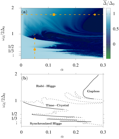
Figure 1: (Color online) (a) Temporal average of superconducting order parameter $\bar{\Delta}$ as a function of amplitude and frequency of the drive, considering a $\lambda-$driving protocol. We have computed $\bar{\Delta}$ using the time window $t\Delta_{0}\in[0,200].$ Dashed orange lines indicate cuts to be show later (Figs. 9,10). The orange dots indicate the parameters where the detailed dynamics is displayed (Fig. 2). They correspond to the different dynamical phases found: Synchronized Higgs (circle), time-crystal (triangle), Rabi-Higgs (square) and gapless (rhombus). (b) Schematic representation of the phase diagram showing the dominant phases in each region. Dashed curves represent continuous phase transitions with fractal-like boundaries while solid lines represent first-order DPTs as shown below.

III Dynamical Phase Diagrams

In this section, we present the dynamical phase diagram with both driving methods and in a wide range of frequency and driving strengths. Previous studies focused on $\lambda$-driving and the subgap regime Ojeda Collado et al. (2021a) or specific frequencies Ojeda Collado et al. (2018, 2020).

A first screening of the phase diagram can be obtained Ojeda Collado et al. (2021a) using the time-averaged superconducting order parameter $\bar{\Delta}$ as dynamical order parameter. In Fig. 1 we show a false color map of $\bar{\Delta}$ as a function of the amplitude and frequency of the drive for the $\lambda-$driving protocol. At first look, there are two main regions that can be easily distinguished: in the light blue regions the average of the superconducting order parameter is near the equilibrium value ($\bar{\Delta}\approx\Delta_{0}$) while regions with zero order parameter average (ZOPA) appear in dark blue. We identify four different dynamical phases within these regions, which are schematized and labeled in panel (b). However, these need a more refined analysis to be distinguished, as explained below.

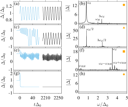
Figure 2: (Color online) Representative dynamical phases for the highlighted parameters (filled dots) of Fig. 1 (a). In the left column we show the dynamics (transient in blue and steady state in black) and the FT in the corresponding right panel. For the Fourier analysis, we consider a long time window $t\Delta_{0}\in[200,2500]$ to obtain better resolution. (a, b) Synchronized Higgs mode phase in which the system responds with the Higgs frequency $\omega_{H}=2\bar{\Delta}$. (c, d) Time-crystal phase as a consequence of a time-translational symmetry breaking in which the order parameter shows period-doubling oscillations. (e, f) Rabi-Higgs mode phase, in which the superconducting order parameter oscillates with a low fundamental frequency $\omega_{RH}$. Also in this regime, the Higgs mode $\omega_{H}$ appears as a very low peak in the FT which is not appreciable in the present scale but in the log scale used in Fig 9. (g,h) Gapless regime where $\Delta(t)$ goes very rapidly to zero and remains zero over time without exhibiting appreciable oscillations.

Two dynamical phases appear for subgap excitations, and two when the system is driven above the gap $\omega_{d}>2\Delta_{0}$. This rather strong distinction could be anticipated as in one case it is not possible to directly excite quasiparticles in the system (for subgap excitations in an off-resonant regime) while for $\omega_{d}>2\Delta_{0}$ it is possible.

For $\omega_{d}<2\Delta_{0}$, dark indentations or “Arnold tongues” appear at $\omega_{d}=2\Delta_{0}/n$, with $n$ a natural number. These are the parametric resonances reported in Ref. Ojeda Collado et al. (2021a). The phase outside the Arnold tongues, labeled “synchronized Higgs”, is characterized by an order parameter quite close to equilibrium (light blue regions). In contrast, for $\omega_{d}>2\Delta_{0}$ the non-ZOPA phases are characterized by a smaller average order parameter. Indeed, the light blue regions are darker when $\omega_{d}>2\Delta_{0}$ than in the opposite case, indicating more quasiparticles excitations in the steady state.

In some regions the phase diagram has a marbled aspect indicating that, in general, different dynamical phases intermix. However, regions with predominance of a given phase can be identified as schematized in the lower panel.

An example of the time evolution and its Fourier transform (FT) for each one of the dynamical phases is shown in Fig. 2. The orange dots allow to associate the parameters of each row with their location in the phase diagram.

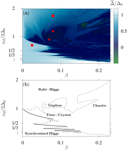
Figure 3: (Color online) (a) Temporal average of superconducting order parameter $\bar{\Delta}$ as a function of amplitude and frequency of the drive considering a DOS-driving protocol. We have computed $\bar{\Delta}$ using the time window $t\Delta_{0}\in[0,200].$ The red dots indicate the parameters used to illustrate the more prominent dynamical phases appearing in the phase diagram: Synchronized Higgs phase (circle), time-crystal phase (triangle), Rabi-Higgs phase (square) and gapless phase (rhombus) (see App. A). (b) Schematic representation of the phase diagram showing the dominant phases in each region. Dashed curves represent continuous phase transitions with fractal-like boundaries while solid lines represent first-order DPTs. In the rightmost part of the phase diagram, dynamical phases intermix in very small regions, forming a chaotic structure.

In the presence of a bath Ojeda Collado et al. (2019, 2020) the system can reach thermodynamic equilibrium and linear-response theory can be applied. In the linear regime Volkov and Kogan (1974); Cea and Benfatto (2014); Ojeda Collado et al. (2018) the time-dependent gap parameter responds with the same frequency of the drive, so the time-translation symmetry properties of the drive are preserved. Here, without a bath, for all the four dynamical phases, this time-translation symmetry preservation does not hold, so these are exquisitely non-linear effects which can occur as prethermal phenomena Ojeda Collado et al. (2021a).

In the synchronized Higgs phase, illustrated in panels (a) and (b) of Fig. 2, the superconducting order parameter oscillates not only with the drive frequency $\omega_{d}$ (and high harmonics) but also with a different and incommensurate fundamental frequency given by $\omega_{H}=2\bar{\Delta}$ (fundamental Higgs frequency). In the time-crystal phase [panels (c) and (d)], after a transient dynamics, period-doubling oscillations are stabilized, indicating a subharmonic response. This is the typical behavior of discrete time-translational symmetry breaking displayed by Floquet time-crystals Else et al. (2016); Yao et al. (2017); Russomanno et al. (2017); Rovny et al. (2018); Yao et al. (2020); Else et al. (2020); Giachetti et al. (2022); Muñoz-Arias et al. (2022). Notice that the drive frequency $\omega_{d}$ does not appear in the FT but the subharmonic response remains locked at $\omega_{d}/2$. This behavior persists under changes in the drive amplitude or frequency Ojeda Collado et al. (2021a) which is the hallmark of time-crystal behavior Yao et al. (2017); Else et al. (2020).

For $\omega_{d}>2\Delta_{0}$ and relatively small perturbation amplitudes $\alpha$, the dynamics shows a slow modulation amplitude on top of the fast oscillations at frequency $\omega_{d}$ [see Fig. 2(e)]. This low frequency mode has been denoted as $\omega_{RH}$ in the FT (f) and corresponds to the Rabi-Higgs mode reported in Ref. Ojeda Collado et al. (2018). In this regime, a subset of pseudospins get synchronized and perform Rabi oscillations with a frequency proportional to the amplitude of the drive. This corresponds again to a time-translation symmetry-breaking subharmonic response. However, the frequency of the mode can be tuned with the external drive, which means that the response lacks “rigidity” and therefore does not qualify as a time-crystal phase according to the standard definitions Yao et al. (2017); Else et al. (2020).

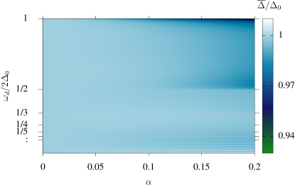
Figure 4: (Color online) Dynamical phase diagram for non-interacting pseudospins. We show the temporal average of the superconducting order parameter in the $\alpha$-$\omega_{d}$ plane for noninteracting pseudospins subject to an oscillating (nonselfconsistent) pseudomagnetic field. In this case, parametric resonances are absent and only a weak feature appears for subgap excitation at $\omega_{d}\approx\Delta_{0}$ and large driving amplitude. This feature becomes visible by zooming the intensity scale to a small window around $\Delta_{0}$ (Notice the different color bar scale respect to the other figures).

Finally, by exciting above the gap with large drive amplitude, the system enters into a gapless regime in which the superconducting order parameter goes to zero very rapidly in time and then remains constant (g). As we shall demonstrate in the following, the fact that $\Delta(t)=0$ does not mean the absence of pairing in the system but a “perfect” dephasing between quasiparticles. Also in this case the response does not have the same periodicity of the drive. However, instead of symmetry breaking in this case there is symmetry restoring (since the response is more symmetric in time) although in a rather trivial way.

The real time evolution shows that for all dynamical phases there are lapses of time in which the superconducting order parameter is larger than the equilibrium value $\Delta_{0}$. This is more evident for the gapless regime (g) in which $\Delta(t)$ surpass $2\Delta_{0}$ at very short times before getting down to zero. However, this value is still below the increase we could expect by considering an adiabatic evolution Seibold et al. (2021) where we use the instantaneous DOS or pairing interaction in the equilibrium gap equation. So this effect is rather trivial and should not be confused with dynamically induced superconductivity.

In Fig. 3 we present the same phase diagram (a) and the corresponding sketch (b) but now by considering the DOS-driving protocol. There are many common characteristics by comparing with Fig. 1. In particular, one sees that parametric resonances for $\omega_{d}<2\Delta_{0}$ are robust features that naturally emerge independently of the protocol details. Indeed, they appear both for periodic drive acting only along the pseudomagnetic field $x-$direction ($\lambda-$driving) or acting along $x$ and $z-$axis at the same time (DOS-driving case). On the other hand, we show that the same dynamical phases appear with some difference in the details of the regions of stability. In contrast to the phase diagram for the $\lambda$ driving case, here, for large perturbation amplitudes ($\beta\gtrsim 0.15$), the dynamical phase diagram becomes more chaotic where all dynamical phases practically coexist in small regions.

For completeness, we show the different dynamics at the red points in Appendix A.

III.1 The crucial role of interactions

The classical parametric oscillator with one degree of freedom Landau and Lifshitz (1976) is the simplest mechanical system to show a subharmonic response, a key ingredient of time-crystal behavior. However, time-crystals are defined also by their many-body nature. Thus, a successful way to build time-crystals is by making several parametric oscillators to interact Heugel et al. (2019); Nicolaou and Motter (2021).

The dynamics of a single pseudospin in an external magnetic field is governed by Bloch equations, which can describe non trivial phenomena as Rabi oscillations. In analogy with the above systems, one can wonder if the subharmonic response is already built before interactions are switch on. To check for this, we solve the EOM [Eq. (7)] with a non-selfconsistent pseudomagnetic field,

$$\bm{b_{\bm{k}}}\left(t\right)=2\left(\Delta_{0}\left[1+\alpha\sin\left(\omega_{d}t\right)\right],0,\xi_{\bm{k}}\right),$$ (14)

starting with the equilibrium initial condition [pseudospins texture of Eq. (6)].

In this case, the phase diagram becomes trivial without any visible Arnold tongues as shown in Fig. 4 where we report a false colour plot of the temporal average of the order parameter defined here as,

$$\bar{\Delta}=\lambda_{0}\sum_{\bm{k}}\bar{S_{\bm{k}}^{x}}.$$ (15)

It shows that differently from Refs. Heugel et al. (2019); Nicolaou and Motter (2021) the subharmonic response is not built in the elementary constituents but it is an emergent phenomenon which appears only after fully taking into account the quasiparticle interactions in the system. We will come back to this problem in Sec. VI where we will show how the system can be mapped to a collection of highly non-linear oscillators.

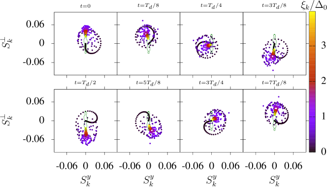
Figure 5: (Color online) We show snapshots, during a time window $T_{d}$, of pseudospins dynamics in the synchronized Higgs mode phase ($\alpha=0.05$ and $\omega_{d}=0.8\Delta_{0}$ corresponding with the parameters used in Fig. 2 (a,b)). On the top of panels, we indicate the time. A pseudospin trajectory for $\xi_{k}\simeq 3\Delta_{0}$ is shown in green. See also Supplementary Video 1.

IV Typical pseudospins trajectories for each dynamical phase

A more refined characterization of the dynamical phases can be obtained by studying the response resolved for each individual pseudospin. Here we show results for the $\lambda-$driving case but DOS-driving yields similar results.

In some cases, the dynamics is more easily analysed in terms of longitudinal and transverse components with respect to the direction of each pseudospin at equilibrium (i.e. without drive). Thus, we define a pseudospin dependent reference frame, hereafter the equilibrium Larmor frame (ELF), introducing the versor along the equilibrium direction,

$$\hat{\bm{e}}^{\parallel}_{\bm{k}}=2{\bm{S}}_{\bm{k}}^{0}=\frac{2}{\omega_{\bm{k}}}(\Delta_{0},0,\xi_{\bm{k}}),$$ (16)

and two transverse directions,

$$\hat{\bm{y}} = (0,1,0),$$ (17)

$$\hat{\bm{e}}^{\perp}_{\bm{k}} = \hat{\bm{y}}\times\hat{\bm{e}}^{\parallel}_{\bm{k}}=\frac{2}{\omega_{\bm{k}}}(\xi_{\bm{k}},0,-\Delta_{0}).$$ (18)

With these definitions the pseudospin deviations from equilibrium, $\delta{\bm{S}}_{\bm{k}}\equiv{\bm{S}}_{\bm{k}}-{\bm{S}}_{\bm{k}}^{0}$, can be decomposed in longitudinal ($\parallel$) and transverse ($\perp$, $y$) components:

$$\delta{\bm{S}}_{\bm{k}}=\delta S_{\bm{k}}^{\parallel}\hat{\bm{e}}^{\parallel}_{\bm{k}}+\delta{S}_{\bm{k}}^{\perp}\hat{\bm{e}}^{\perp}_{\bm{k}}+\delta{S}_{\bm{k}}^{y}\hat{\bm{y}}.$$ (19)

Notice that since the pseudospins are normalized to length 1/2 giving two components specifies the vector up to a sign of the third component.

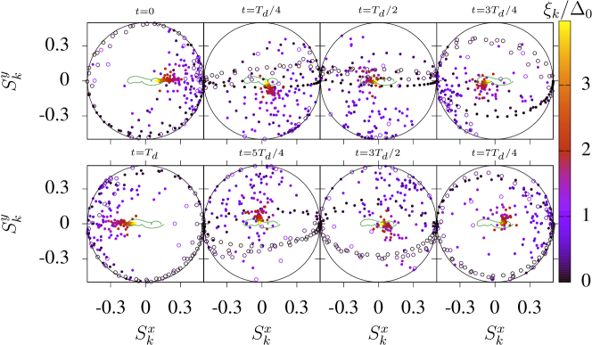
Figure 6: (Color online) Dynamics in the time-crystal phase. We show snapshots, during a time window $2T_{d}$, of pseudospins dynamics in the time-crystal phase. Here, $\alpha=0.05$ and $\omega_{d}=1.64\Delta_{0}$ corresponding with the parameters used in Fig. 2 (c,d). On the top of panels we indicate the time. The green loop points out a typical trajectory of pseudospins (orange dots). Those pseudospins with $S^{z}_{k}>0$ ($S^{z}_{k}<0$) are indicated with filled (empty) dots. See also Supplementary Video 2.

IV.1 Synchronized Higgs phase

Figure 5 shows snapshots of the steady state dynamics for the synchronized Higgs phase in the ELF during a driving period, $T_{d}=2\pi/\omega_{d}$. The color encodes the fermionic energy $\xi_{\bm{k}}$. Notice that because of particle-hole symmetry [Eqs. (II.1)] it is enough to show the pseudospins for $\xi_{\bm{k}}>0$ to specify the full texture. In this dynamical phase, the pseudospins precess very close to its equilibrium position represented by the origin. Pseudospins with quasiparticle energy $\xi_{\bm{k}}\simeq\Delta_{0}$ (purple dots), oscillate with the drive frequency in such a way that they perform a full anticlockwise turn in a drive period $T_{d}$. In contrast, the low-energy pseudospins (black dots) precess more rapidly, so that by $t=3T_{d}/8$ they have performed more than a full turn. Their frequency $2\bar{\Delta}$ corresponds to the Higgs mode. Notice that the loop shape formed by the low-energy pseudospins (in black) preserves its form during the evolution, indicating that there is no significant dephasing. Indeed, synchronization of these pseudospins yields the main contribution to the Higgs mode. Because of particle-hole symmetry, the pseudospin at the Fermi level can not be excited by the drive. In general one can show that the deviation from the equilibrium position should decrease for low-energy pseudospins (black dots) as indeed observed.

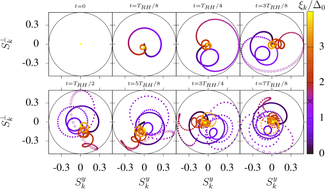
Figure 7: (Color online) Dynamics in the Rabi-Higgs phase. We show snapshots, during the first Rabi period $T_{RH}$, of pseudospins dynamics in the Rabi-Higgs regime ($\alpha=0.12$ and $\omega_{d}=3.5\Delta_{0}$ corresponding with the parameters used in Fig. 2 (e,f)). On the top of panels, we indicate the time. Those pseudospins with $S^{z}_{k}>0$ ($S^{z}_{k}<0$) are indicated with filled (empty) dots. The cross in the colour bar indicates the $\xi^{*}_{\bm{k}}$ satisfying the resonance condition $\omega_{L}(\xi_{\bm{k}}^{\ast})=\omega_{d}$. See also Supplementary Video 3.

IV.2 Discrete time-crystal phase

We now turn to the discrete time-crystal phase. Because $\bar{\Delta}=0$ is very far from the equilibrium value $\Delta_{0}$, it is convenient to use a Cartesian frame instead of the ELF. Figure 6 shows the dynamics during a 2$T_{d}$ time window. Full (open) symbols indicate $S^{z}_{\bm{k}}>0$ ($S^{z}_{\bm{k}}<0$). The high-energy pseudospins (red-yellow dots) precess around the instantaneous pseudomagnetic field describing a loop (green line) and contributing self-consistently to build the time-dependent order parameter. Very low energy pseudospins have a nearly maximal component in the $xy$ plane in the first frame, indicating strong pairing correlations but with incoherent phases. This initial circular feature becomes an ellipse at subsequent times, corresponding to a ring that rotates nearly rigidly along the $x$ axis of the Bloch sphere. Spins at intermediate energies (violet-orange dots) interpolate between these two behaviors, contributing significantly to the time dependent $\Delta(t)$. Indeed, the red and violet cloud is on the right side of the frame at $t=0$ contributing to a positive $\Delta$ [cf. Eq. (4)] and after one drive period has shifted to the left, yielding the sign alternation of $\Delta$ in one drive period as shown in Fig. 3(c). After two drive periods, the pattern goes approximately back to the original distribution, consistently with the behavior of the order parameter.

IV.3 Rabi-Higgs phase

Turning now to the Rabi-Higgs phase, since the order parameter is close to equilibrium, it is convenient to use the ELF once again. In Fig. 7 we show several texture snapshots during the first Rabi-Higgs period $T_{RH}$. At $t=0$ (equilibrium) the pseudospins texture corresponds to all pseudospins at the origin by definition. For $t=T_{RH}/2$ we have the inversion phenomenon in which a subset of pseudospins (empty dots) get inverted with respect to its fermionic energy. In other words, they have an instantaneous negative $S^{z}_{\bm{k}}$ while $\xi_{\bm{k}}>0$. Since the $z$ component of the pseudospin encodes the charge, this corresponds to an inversion of the quasiparticle population. The pseudospins that get inverted satisfy the resonance condition $\omega_{d}=\omega_{L}(\xi_{\bm{k}}^{\ast})$ with $\omega_{L}(\xi_{\bm{k}})=2\sqrt{\xi_{\bm{k}}^{2}+\Delta_{0}^{2}}$, the natural Larmor frequency. We indicate this fermionic energy $\xi_{\bm{k}}^{\ast}$ with a cross in the colour bar. After one full Rabi period, this inversion gets largely diminished. In the steady state one observes a periodic oscillation of the population as discussed in Ref. Ojeda Collado et al. (2018).

IV.4 Gapless phase

Finally, for the gapless phase it is convenient to go back to the Cartesian frame. In Fig. 8 we show texture snapshots at short times. We see that after a fast transient, the pseudospins start to roll up around the coordinate origin with the shape of a spiral. This unveils that the gapless phase consists in strong pairing correlations, i.e. for several pseudospins $S_{\bm{k}}^{x}\neq 0$, but with Cooper pairs which are not phase-coherent. So the sum of the $x$ components yields a zero gap. This is not, however, a chaotic state, but the ZOPA is a consequence of a very orderly movement of pseudospins consistent with the unitary evolution of the state.

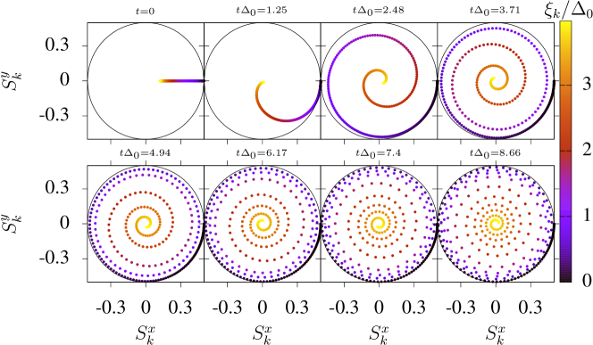
Figure 8: (Color online) Dynamics in the gapless regime. We show snapshots, during the transient to the gapless behavior, of pseudospins dynamics in the gapless phase ($\alpha=0.27$ and $\omega_{d}=3.5\Delta_{0}$ corresponding with the parameters used in Fig. 2 (g,h)). On the top of panels, we indicate the time. See also Supplementary Video 4.

V Dynamical Phase Transitions

In order to characterize the order of the different DPTs, we analyse the behaviour of the system along the dashed vertical line in Fig. 1 (a) corresponding to $\alpha=0.05$. Figure 9 (a) shows the FT of the time-dependent superconducting order parameter as a function of $\omega_{d}$ while panel (b) shows its long term average in the steady state, $\bar{\Delta}$.

In the adiabatic limit ($\omega_{d}\ll 2\Delta_{0}$), the FT shows a clear peak at $\omega_{d}$ resulting in the strong linear orange feature in Figure 9(a) as expected from linear response. A weaker feature appears at $2\omega_{d}$ corresponding to the allowed Ojeda Collado et al. (2020) second harmonic generation. Increasing $\omega_{d}$, the dynamical order parameter $\bar{\Delta}$ [panel (b)] shows discontinuities near $\omega_{d}/(2\Delta_{0})=1/2$ and $\omega_{d}/(2\Delta_{0})=1/3$ corresponding to first order DPTs associated to low $\alpha$ precursors of the Arnold tongues [c.f. Fig. 1 (a)]. Inside the dynamical phases with finite $\bar{\Delta}$, well-defined peaks appear at $\omega_{H}$ and $\omega_{H}\pm\omega_{d}$ associated with the synchronized Higgs mode. The dotted lines in panel (a) are $2\bar{\Delta}$ (large dots) and $2\bar{\Delta}\pm\omega_{d}$ (small dots), showing that the frequency of the Higgs mode is locked at $2\bar{\Delta}$. This can be seen as incommensurate time-crystal behavior similar to Ref. Homann et al. (2020).

For $2\omega_{d}$ higher than the minimum of the effective continuum $2\bar{\Delta}$, the second harmonic of the drive is resonant with the quasiparticles. This produces a proliferation of excitations resulting in a suppression of the average gap as shown in Fig. 9 (b) for $\omega_{d}/2\Delta_{0}\approx 1/2$. As $\omega_{d}$ decreases, the $2\omega_{d}$ resonance approaches the quasiparticle minimum and the range of resonant quasiparticles gets cutoff. At some point, there are not enough quasiparticles with $2\sqrt{\xi_{\mathbf{k}}^{2}+\bar{\Delta}^{2}}\approx 2\omega_{d}$ to suppress the gap and a new steady state is found, in which the Higgs mode frequency increases discontinuously with $\omega_{H}>2\omega_{d}$. Thus, the line $\omega=2\omega_{d}$ intersects the jump of $\omega_{H}$ in Fig. 9 (a). A similar mechanism applies to the weaker transition at lower frequency, with the third harmonic resonance and the line $\omega=3\omega_{d}$ intercepting the jump of $\omega_{H}$.

While the previous two DPTs are among phases with the same symmetry, the third discontinuity at $\omega_{d}/2\Delta_{0}\simeq 0.8$ represents a DPT between qualitatively distinct phases: gaped on the left and ZOPA on the right. The ZOPA phase corresponds to the $n=1$ Arnold tongue and is bounded by the solid vertical lines in Fig. 10 (a). Inside this region ($0.8\lesssim\omega_{d}/2\Delta_{0}\lesssim 0.9$), a commensurate time-crystal appears with a doubling of the period of the drive. The persistence of the order parameter oscillation at $\omega_{d}/2$ in this finite region indicates that the period doubling is not accidental. As discussed in Ref. Ojeda Collado et al. (2021a) this is also true changing $\alpha$ in a finite range. Thus, we confirm again that this state satisfies the rigidity criteria Yao et al. (2017) for time-crystalline behaviour.

Both transitions bounding the time-crystal phase are first order. The upper edge of the tongue has a fractal like appearance Ojeda Collado et al. (2021b) which has been noticed also in related models Giachetti et al. (2022). Even inside the tongue, as already mentioned, marbled textures appear where $\bar{\Delta}$ becomes nonzero. In these cases, as illustrated in the rightmost part of Fig. 9 (a), the time crystal is lost and the system switches to a phase in which time-translational symmetry is recovered at $\omega_{d}/2\Delta_{0}\sim 0.9$ (marked with a second vertical line in the figure). For higher frequencies, the system enters a complex regime in which our numerical calculations show instabilities. In general, we find that when $\bar{\Delta}\simeq 0$ (for $\omega_{d}<2\Delta_{0}$) a time-crystal phase emerges.

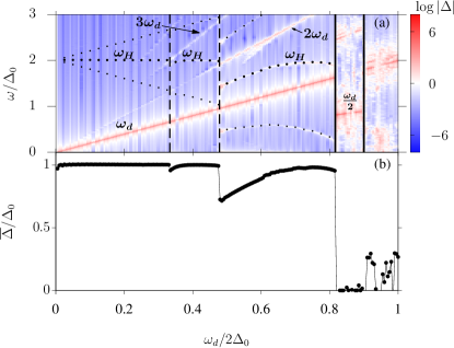
Figure 9: (Color online) (a) Characterization of DPTs thought a false colour plot of the superconducting response in the frequency domain vs. driving frequency, $\omega_{d}$ for $\alpha=0.05$. We used $t\Delta_{0}\in[1500,2500]$ for high frequency resolution. Large and small dots represent $2\bar{\Delta}$ (shown also in b) and $2\bar{\Delta}\pm\omega_{d}$ respectively. These values are taken from the real time gap dynamics $\Delta(t)$. Notice that they match peaks in the FT. Vertical lines indicate equal symmetry (dashed) and different symmetry (full) first order DPTs. (b) Average of superconducting order parameter vs. drive frequency.

Now we discuss on the DPTs along the horizontal dashed line $\omega_{d}=3.5\Delta_{0}$ shown in Fig. 1 (a). Figure 10 (a) shows the FT map of $\Delta(t)$ for different values of the drive amplitude $\alpha$. For extremely weak perturbation amplitudes, the system essentially responds with the drive frequency and the Higgs mode $\omega_{H}=2\bar{\Delta}$ as occurs for drive frequencies below the gap. As soon as we increase the drive amplitude $\alpha$, the Rabi-Higgs mode $\omega_{RH}$ appears in the spectrum, whose frequency increases linearly by increasing $\alpha$. At the same time, satellites at frequencies $\omega_{d}\pm n\omega_{RH}$ with $n=1,2$ appear in the FT. Slightly less prominent, but still appreciable, are peaks at $\omega_{H}\pm\omega_{RH}$ witnessed by white branches near to $\omega_{H}$ that linearly grow with $\alpha$.

Increasing even more the amplitude, it is clear from Fig 10 (a) that there is a critical value $\alpha$ (marked by the vertical dashed line) in which the Rabi-Higgs starts to soften. It is more clearly seen in the satellites peaks $\omega_{d}\pm\omega_{RH}$. This is an anomalous behaviour, taking into account that a conventional Rabi frequency increases by increasing the amplitude of the drive. Increasing even more the drive, the Rabi-Higgs and Higgs modes disappear and the system enters into a gapless regime (blue area in panel a). In this case, not only $\bar{\Delta}=0$ but also $\Delta=0$ (i.e. the superconducting order parameter is zero over time without exhibiting oscillations). This DPT is indicated by a solid vertical line. In contrast to the first order DPTs described in Fig. 9, here both the dynamics and the order parameter $\bar{\Delta}$, shown in panel (b), point to a second order DPT with the characteristic “critical slowing down” near the transition point.

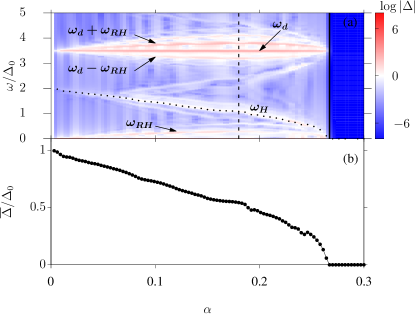
Figure 10: (Color online) (a) The superconducting response in the frequency domain vs. the amplitude of the drive $\alpha$ for $\omega_{d}=3.5\Delta_{0}$. We used $t\Delta_{0}\in[10,200]$ to compute the average and the FT. Small dots represent $2\bar{\Delta}$ (shown also in b). These values are taken from the real time gap dynamics $\Delta(t)$ and match peaks in the FT. Dashed vertical line indicates the $\alpha$ value for which the Rabi-Higgs mode start to soften. Full vertical line instead points out the second order DPTs to a gapless regime. The blue region on the right corresponds to $\Delta=0$. (b) Average of superconducting order parameter vs. drive amplitude.

VI Mapping to classical dynamics

In order to investigate the origin of the parametric resonances found numerically in Fig. 1 it is useful to map the BCS dynamics to classical anharmonic oscillators Sciolla and Biroli (2011). This can be done because the dynamics of pseudospins can be mapped to the dynamics of a collection of classical spins $\bm{S}_{\bm{k}}$. Such dynamic is governed by the Hamilton equations $\partial_{t}\bm{S}_{{\bm{k}}}=\left\{\mathcal{H},\bm{S}_{{\bm{k}}}\right\}$ using the usual Poisson brackets $\left\{S_{{\bm{k}}}^{\mu},S_{{\bm{k}}^{\prime}}^{\nu}\right\}=-\varepsilon_{\mu\nu\eta}\delta_{{\bm{k}},{\bm{k}}^{\prime}}S_{{\bm{k}}}^{\eta}$ for angular momenta where $\mu,\nu,\eta$ represents the $x,y,z$ component and $\varepsilon_{\mu\nu\eta}$ is the Levi-Civita tensor.

Alternatively one can derive the BCS time-dependent equations from a variational principle, requiring that the wave-function has a BCS form at each instant of time and using the elements of the generalized one-particle density matrix as dynamical variables  Blaizot and Ripka (1986); Schiró and Fabrizio (2010); Sciolla and Biroli (2011); Bünemann et al. (2013); Seibold et al. (2021). For each pair ($\bm{k}\uparrow$, $-\bm{k}\downarrow$), four expectation values of the one-particle density matrix need to be considered, corresponding to the four operators appearing on the right-hand side of Eqs. (2).

One can show that the density matrix derives from a BCS state if and only if the generalized matrix is idempotent Blaizot and Ripka (1986). It is easy to show that this is equivalent to the following constraints,

$$\left(S_{{\bm{k}}}^{x}\right)^{2}+\left(S_{{\bm{k}}}^{y}\right)^{2}+\left(S_{{\bm{k}}}^{z}\right)^{2}=1/4,$$ (20)

$$\langle\hat{c}_{\bm{k}\uparrow}^{\dagger}\hat{c}_{\bm{k}\uparrow}\rangle=\langle\hat{c}_{-\bm{k}\downarrow}^{\dagger}\hat{c}_{-\bm{k}\downarrow}\rangle.$$ (21)

We can use Eq. (21) to reduce the dynamical variables for a pair ($\bm{k}\uparrow$, $-\bm{k}\downarrow$) to three variables which can then be taken as the pseudospin expectation values $S_{{\bm{k}}}^{x}$, $S_{{\bm{k}}}^{y}$, $S_{{\bm{k}}}^{z}$ with the constraint Eq. (20).

In this formalism, the time-dependent expectation value of the quantum Hamiltonian plays the role of a classical Hamiltonian and can be obtained from Eq. (1) replacing operators by their expectation values in the instantanous BCS wave-function. Adding the constraint Eq. (20) with Lagrange multipliers $\omega_{\bm{k}}$, the classical Hamiltonian reads,

$$\mathcal{H} = -\sum_{\bm{k}}2S^{z}_{\bm{k}}\xi_{\bm{k}}-\lambda\sum_{{\bm{k}},{\bm{k}}^{\prime}}(S^{x}_{\bm{k}}S^{x}_{{\bm{k}}^{\prime}}+S^{y}_{\bm{k}}S^{y}_{{\bm{k}}^{\prime}})$$

$$- 2f\sum_{\bm{k}}S^{x}_{\bm{k}}+\sum_{\bm{k}}\omega_{\bm{k}}\left[(S^{x}_{\bm{k}})^{2}+(S^{y}_{\bm{k}})^{2}+(S^{z}_{\bm{k}})^{2}-\frac{1}{4}\right]$$

The third term is an additional external pairing field which couples linearly with the order parameter and which we added for latter use. As before, driving will be introduced by making $\xi_{{\bm{k}}}$, $\lambda$, or $f$, time-dependent. Here we concentrate on the $\lambda$-driving and discuss briefly $f$-driving. The DOS-driving protocol can be treated similarly.

It is useful to use as dynamical variables the deviation (not necessarily small) $\delta S^{\mu}_{\bm{k}}$ defined as $S^{\mu}_{\bm{k}}\equiv S^{\mu,0}_{\bm{k}}+\delta S^{\mu}_{\bm{k}}$, with $S^{\mu,0}_{\bm{k}}$ the equilibrium BCS state. We also write the time dependence of the pairing interaction as an average value $\lambda_{0}$ plus a fluctuation, $\lambda=\lambda_{0}+\delta\lambda$. The Hamiltonian can be written as $\mathcal{H}=E_{0}+\delta\mathcal{H}$ with $E_{0}$ the equilibrium BCS ground state energy and with the fluctuating part,

$$\delta\mathcal{H}= - 2\sum_{\bm{k}}\delta S^{z}_{\bm{k}}\xi_{\bm{k}}-\delta\lambda\sum_{{\bm{k}},{\bm{k}}^{\prime}}(S^{x,0}_{\bm{k}}S^{x,0}_{{\bm{k}}^{\prime}}+S^{y,0}_{\bm{k}}S^{y,0}_{{\bm{k}}^{\prime}})$$

$$- 2(\lambda_{0}+\delta\lambda)\sum_{{\bm{k}},{\bm{k}}^{\prime}}(\delta S^{x}_{\bm{k}}S^{x,0}_{{\bm{k}}^{\prime}}+\delta S^{y}_{\bm{k}}S^{y,0}_{{\bm{k}}^{\prime}})$$

$$- (\lambda_{0}+\delta\lambda)\sum_{{\bm{k}},{\bm{k}}^{\prime}}(\delta S^{x}_{\bm{k}}\delta S^{x}_{{\bm{k}}^{\prime}}+\delta S^{y}_{\bm{k}}\delta S^{y}_{{\bm{k}}^{\prime}})$$

$$+ \sum_{\bm{k}}\omega_{\bm{k}}[2S^{x,0}_{\bm{k}}\delta S^{x}_{\bm{k}}+2S^{y,0}_{\bm{k}}\delta S^{y}_{\bm{k}}+2S^{z,0}\delta S^{z}_{\bm{k}}$$

$$+ (\delta S^{x}_{\bm{k}})^{2}+(\delta S^{y}_{\bm{k}})^{2}+(\delta S^{z}_{\bm{k}})^{2}]-2f\sum_{{\bm{k}}}\delta S^{x}_{\bm{k}}.$$

The saddle point condition requires that linear-variations vanish which, by setting $f=\delta\lambda=0$, yields the equilibrium mean-field equations,

$$-\Delta^{x}_{0}+\omega_{\bm{k}}S^{x,0}_{\bm{k}} = 0,$$ (24)

$$-\Delta^{y}_{0}+\omega_{\bm{k}}S^{y,0}_{\bm{k}} = 0,$$ (25)

$$-\xi_{\bm{k}}+\omega_{\bm{k}}S^{z,0}_{\bm{k}} = 0,$$ (26)

with $\Delta^{\mu}_{0}=\lambda_{0}\sum_{\bm{k}}S^{\mu,0}_{\bm{k}}$ which can be readily solved for $S^{\mu,0}_{\bm{k}}$. Without loss of generality, we take $\Delta_{0}^{x}=\Delta_{0}$ and $\Delta_{0}^{y}=0$. Applying the constraint to the stationary state, one finds that the Lagrange multiplier is given by the equilibrium Larmor frequency, $\omega_{\bm{k}}=\omega_{L}(\xi_{\bm{k}})=2\sqrt{\xi^{2}_{\bm{k}}+\Delta_{0}^{2}}$. The negative root can be discarded as it yields the unphysical sign of $S^{z,0}_{\bm{k}}$. Solving for the spin components, yields Eq. (6).

Using the saddle point condition, the Hamiltonian has terms up to cubic in fluctuations and is given by

$$\delta\mathcal{H}= - (\lambda_{0}+\delta\lambda)\sum_{{\bm{k}},{\bm{k}}^{\prime}}(\delta S^{x}_{\bm{k}}\delta S^{x}_{{\bm{k}}^{\prime}}+\delta S^{y}_{\bm{k}}\delta S^{y}_{{\bm{k}}^{\prime}})$$

$$+ \sum_{\bm{k}}\omega_{\bm{k}}[(\delta S^{x}_{\bm{k}})^{2}+(\delta S^{y}_{\bm{k}})^{2}+(\delta S^{z}_{\bm{k}})^{2}]$$

$$- 2\left(\frac{\delta\lambda}{\lambda_{0}}\Delta_{0}+f\right)\sum_{{\bm{k}}}\delta S^{x}_{\bm{k}},$$

where we droped terms linear in $\delta\lambda$ which do not affect the EOM. It is useful to transform the Hamiltonian to the ELF of Eq. (19) to obtain,

$$\delta\mathcal{H} = \sum_{\bm{k}}\omega_{\bm{k}}[(\delta S^{y}_{\bm{k}})^{2}+(\delta S^{\perp}_{\bm{k}})^{2}+(\delta S^{\parallel})^{2}]$$ (28)

$$- (\lambda_{0}+\delta\lambda)\sum_{{\bm{k}},{\bm{k}}^{\prime}}\left(4\frac{\xi_{\bm{k}}\xi_{{\bm{k}}^{\prime}}}{\omega_{\bm{k}}\omega_{{\bm{k}}^{\prime}}}\delta S^{\perp}_{\bm{k}}\delta S^{\perp}_{{\bm{k}}^{\prime}}+\delta S^{y}_{\bm{k}}\delta S^{y}_{{\bm{k}}^{\prime}}\right)$$

$$- 4\left(\frac{\delta\lambda}{\lambda_{0}}\Delta_{0}+f\right)\sum_{{\bm{k}}}\frac{\xi_{\bm{k}}}{\omega_{\bm{k}}}\delta S^{\perp}_{\bm{k}}.$$

VI.1 Harmonic approximation

So far, the treatment is exact. We now proceed by introducing some approximations. First, one can use the constraint to show that longitudinal fluctuations are higher order compared to transverse ones (which can be also seen from a geometric argument). Thus, we neglect $\delta S_{\bm{k}}^{\parallel}$ in the first term of Eq. (28). Defining canonical variables as $p_{\bm{k}}=\sqrt{2}\delta S^{y}_{\bm{k}}$ and $q_{\bm{k}}=\sqrt{2}\delta S^{\perp}_{\bm{k}}$ the energy reads,

$$\delta\mathcal{H} = \frac{1}{2}\sum_{\bm{k}}\omega_{\bm{k}}(p_{\bm{k}}^{2}+q_{\bm{k}}^{2})$$ (29)

$$- (\lambda_{0}+\delta\lambda)\sum_{{\bm{k}},{\bm{k}}^{\prime}}\left(2\frac{\xi_{\bm{k}}\xi_{{\bm{k}}^{\prime}}}{\omega_{\bm{k}}\omega_{{\bm{k}}^{\prime}}}q_{\bm{k}}q_{{\bm{k}}^{\prime}}+\frac{1}{2}p_{\bm{k}}p_{{\bm{k}}^{\prime}}\right)$$

$$- 2\sqrt{2}\left(\frac{\delta\lambda}{\lambda_{0}}\Delta_{0}+f\right)\sum_{{\bm{k}}}\frac{\xi_{\bm{k}}}{\omega_{\bm{k}}}q_{\bm{k}}$$

which maps the problem to a set of harmonic oscillators with long-range interactions depending on the quasiparticle energy $\xi_{\bm{k}}$. The Larmor frequency $\omega_{L}(\xi_{\bm{k}})$ plays the role of natural frequencies of the oscillators, giving rise to a DOS in frequency space peaking at $2\Delta_{0}$, consistent with the identification of $\omega_{0}=2\Delta_{0}$ as the “natural frequency” of oscillation of the superconducting system Ojeda Collado et al. (2021a).

Setting $f=0$, one can check that the Hamilton EOM,

$$\dot{q}_{\bm{k}}=\frac{\partial\mathcal{H}}{\partial p_{\bm{k}}},\ \ \ \ \ \ \dot{p}_{\bm{k}}=-\frac{\partial\mathcal{H}}{\partial q_{\bm{k}}}$$ (30)

reproduce the linearized version of Eq. 7.

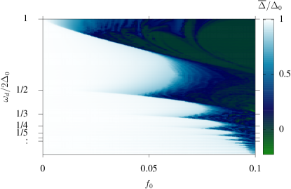
Figure 11: (Color online) Dynamical phase diagram for periodic driving by an external pairing field. We show the temporal average of the superconducting order parameter in the $f_{0}$-$\omega_{d}$ plane for the case of an external paring field drive.

Fluctuations in $\lambda$ couple linearly with the canonical variables [last term in Eq. (29)] and with quadratic fluctuations of canonical variables (second term). In analogy with a single classical parametric oscillator Landau and Lifshitz (1976), it is tempting to attribute parametric resonances to the coupling with quadratic fluctuations. However, this can be excluded in the following way. We set $\delta\lambda=0$ and consider periodic driving in $f=f_{0}\sin(\omega_{d}t)$. From Eq. (29), we see that this driving is equivalent to the linear coupling with $\delta\lambda$ (for that term). Fig. 11 shows the phase diagram computed with the original Hamiltonian Eq. (VI) but with $f$ as the only time-dependent perturbation. In this case, one obtains similar Arnold tongues which reveals that the coupling of $\delta\lambda$ with quadratic fluctuations is not essential to obtain the parametric resonances. This result could be anticipated from the following argument. Since quadratic fluctuations of canonical variables couple linearly with $\delta\lambda$ [c.f. Eq. (29)], the analogy with a single parametric oscillator would yield parametric resonances at $\omega_{d}=2\omega_{0}/n=4\Delta_{0}/n$ which is not consistent with the resonances obtained numerically [Fig. 1 (a)] which satisfy instead, $\omega_{d}=\omega_{0}/n=2\Delta_{0}/n$.

We will see that the linear coupling of $\delta\lambda$ with canonical variables [last term in Eq. (29)] plays a fundamental role in the emergence of the parametric resonances. This does not occur through the direct coupling with the pseudospins fluctuations but indirectly through the effect of higher order non-linearities.

VI.2 Higher orders

Writing the constraint on the pseudospins lenght as $2{\bm{S}}_{\bm{k}}^{0}.\delta{\bf S}_{\bm{k}}+|\delta{\bf S}_{\bm{k}}|^{2}=\delta S_{\bm{k}}^{\parallel}+|\delta{\bf S}_{\bm{k}}|^{2}=0$, we can eliminate longitudinal fluctuations in favour of transverse ones,

$$\frac{1}{2}+\delta S_{\bm{k}}^{\parallel}=\pm\frac{1}{2}\sqrt{1-4(\delta S^{y}_{\bm{k}})^{2}+(\delta S^{\perp}_{\bm{k}})^{2}},$$ (31)

where the left-hand side is nothing but $S_{\bm{k}}^{\parallel}$. We see that for the solution to be real $(\delta S^{y}_{\bm{k}})^{2}+(\delta S^{\perp}_{\bm{k}})^{2}<1/4$ and two solutions are possible, one in which $S_{\bm{k}}^{\parallel}>0$ (ferro alignment) and one in which $S_{\bm{k}}^{\parallel}<0$ antiferro alignment. Although both solutions are needed for the full dynamics, for the time being we restrict to ferro-alignment which is the relevant solution for not too large deviations.

Considering only the $\lambda$-driving and using canonical variables $q_{\bm{k}}$ and $p_{\bm{k}}$, the Hamiltonian reads,

$$\delta\mathcal{H} = \sum_{\bm{k}}\frac{\omega_{\bm{k}}}{2}\left(1-\sqrt{1-2(p_{\bm{k}}^{2}+q_{\bm{k}}^{2})}\right)$$ (32)

$$- (\lambda_{0}+\delta\lambda)\sum_{{\bm{k}},{\bm{k}}^{\prime}}\left(2\frac{\xi_{\bm{k}}\xi_{{\bm{k}}^{\prime}}}{\omega_{\bm{k}}\omega_{{\bm{k}}^{\prime}}}q_{\bm{k}}q_{{\bm{k}}^{\prime}}+\frac{1}{2}p_{\bm{k}}p_{{\bm{k}}^{\prime}}\right)$$

$$- 2\sqrt{2}\frac{\delta\lambda}{\lambda_{0}}\Delta_{0}\sum_{\bm{k}}\frac{\xi_{\bm{k}}}{\omega_{\bm{k}}}q_{\bm{k}}.$$

where again one can check that Hamilton equations yield the correct EOM.

Expanding the square root in a Taylor series, the first term in Eq. (32) can be written as a collection of anharmonic oscillators, $\sum_{\bm{k}}\frac{\Omega_{\bm{k}}}{2}(p_{\bm{k}}^{2}+q_{\bm{k}}^{2}),$ with a time-dependent self-consistently determined natural frequency,

$$\Omega_{\bm{k}}(t)=\omega_{\bm{k}}\left[\right.1+\frac{1}{2}(p_{\bm{k}}^{2}+q_{\bm{k}}^{2})+\frac{1}{2}(p_{\bm{k}}^{2}+q_{\bm{k}}^{2})^{2}$$

$$+\frac{5}{8}(p_{\bm{k}}^{2}+q_{\bm{k}}^{2})^{3}+\ldots\left.\right].$$ (33)

Following Ref. [Landau and Lifshitz, 1976] we can analyse nonlinearities iteratively. Treating the last term in Eq. (32) in linear response Ojeda Collado et al. (2018) one obtains that for a drive frequency $\omega_{d}$, the quadratic terms respond as $(p_{\bm{k}}^{2}+q_{\bm{k}}^{2})\propto\cos{2\omega_{d}t}$ which implies that the natural frequency $\Omega_{\bm{k}}$ is “pumped” with frequency $\omega_{p}=2\omega_{d}$. Thus, using the fact that a classical oscillator has parametric resonances at $\omega_{d}=2\omega_{0}/n$, one expects resonances at $\omega_{d}=2\Delta_{0}/n$ in the BCS system, as indeed found. The identification of the pump-mechanism and the explanation of the factor of two in the resonance series is the main result of this section. We remark that this ingredient alone is not enough to explain the parametric resonances. Indeed, the non-linear effects described arise from the constraint while in Sec. III.1 we showed that interactions, represented here by the second line in Eq. (32) are essential to stabilize parametric resonances. Furthermore, restricting to the “ferro” alignment root in Eq. (32) is not enough in the parametric resonance regime as numerically we find that the dynamics explore both roots [see Fig. 6]. On the other hand, these considerations, do not affect the conclusion that the leading pump frequency for the oscillators is at $\omega_{p}=2\omega_{d}$ instead of $\omega_{d}$ as adding more non-linearites can only produce higher multiples of $\omega_{d}$.

VII Summary and Conclusions

We have presented a comprehensive dynamical phase diagram for a periodically driven BCS condensate using different driving protocols. We concentrated on superconducting/superfluid phases but our results are valid for any phase for which a BCS description is valid in the time regime before energy relaxation process take place in the system. This includes weak-coupling spin and charge density waves which can also be mapped to the BCS model.

We numerically demonstrated that the existence of four dynamical phases and parametric resonances are quite robust to changes in the protocol. To a large extent, the phase diagram can be said universal. We expect the main features to remain, also, for more complicated drives, which for example may be anisotropic on the Fermi surface and depend on light polarization acting as drive.

A detailed analysis of the evolution of the pseudospin textures (Figs. 5-8) allowed to visualize how, the many-body system spontaneously self-organize in momentum space in sectors with different dynamics. For the gapless phase, our analysis revealed a remarkable degree of order and symmetry in this, apparently, unbroken symmetry phase.

Our study allowed to identify the order of the phase transitions. Roughly speaking, parametric resonances at $2\Delta_{0}/n$ can be seen as multiphoton process with $n$ photons reaching the gap. Continuous excitation produces a depletion of the gap which lowers the threshold for excitation. This provides a feedback loop that explains the first order transitions in the lower edge of the Arnold tongues. Second order phase transitions also arise by increasing the intensity of the drive from the Rabi-Higgs to the gapless phase. This is accompanied by a critical slowing down of the dynamics. Thus, the Rabi-Higgs frequency first follows the common expectation for a Rabi mode; its frequency increases with dive strength. For large driving strength it switches to an anomalous regime in which its frequency decreases with strength.

For subgap excitations, by combining different driving protocols and mapping to a system of non-linear oscillators, we showed that the mechanism of parametric pump can be traced back to the non-linearity in the system due to the constraint on the length of pseudospins. Furthermore, we demonstrated that to take into account interactions self-consistently is an essential ingredient to obtain parametric resonances. In other words, they constitute an emergent phenomenon of the many-body system.

Regarding experimental realizations, while the present model neglects the presence of a bath, we have previously shown that, parametric resonances and time-crystal behaviour, appear at very early times in the dynamics Ojeda Collado et al. (2021a). In the presence of a finite decoherence time, they may be observed as a prethermal transient in the dynamics. Proposed realizations in the solid state include THz excitations and a phonon assisted $\lambda$ driving mechanism Ojeda Collado et al. (2018). Ultracold atoms are also very interesting platforms which are inherently much less affected by the environment (lattice vibrations are not present). Furthermore, they offer a large degree of parameter manipulation, making them ideal candidates to study the driven BCS system Behrle et al. (2018). Yet another promising platform to observe the present phenomena is a cavity-QED simulator, where Anderson’s pseudospins model can be directly studied Lewis-Swan et al. (2021). Our work is an invitation to exploit these platforms to experimentally explore the fascinating time-translational symmetry breaking phases of periodically driven BCS systems.

Appendix A Example of Dynamics for DOS-driving

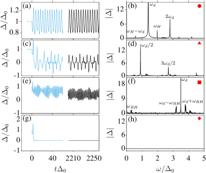
Figure 12: (Color online) The same of Fig. 2 for the parameters indicated in the panel (b) of Fig. 1.

References

- Oka and Kitamura (2019) Takashi Oka and Sota Kitamura, “Floquet Engineering of Quantum Materials,” Annu. Rev. Condens. Matter Phys. 10, 387–408 (2019), arXiv:1804.03212 .
- Bukov et al. (2015) Marin Bukov, Luca D’Alessio, and Anatoli Polkovnikov, “Universal high-frequency behavior of periodically driven systems: From dynamical stabilization to Floquet engineering,” Adv. Phys. 64, 139–226 (2015).
- Claeys et al. (2019) Pieter W. Claeys, Mohit Pandey, Dries Sels, and Anatoli Polkovnikov, “Floquet-Engineering Counterdiabatic Protocols in Quantum Many-Body Systems,” Phys. Rev. Lett. 123, 90602 (2019), arXiv:1904.03209 .
- Meinert et al. (2016) F. Meinert, M. J. Mark, K. Lauber, A. J. Daley, and H.-C. Nägerl, “Floquet Engineering of Correlated Tunneling in the Bose-Hubbard Model with Ultracold Atoms,” Phys. Rev. Lett. 116, 205301 (2016), arXiv:1602.02657 .
- Eisert et al. (2015) J. Eisert, M. Friesdorf, and C. Gogolin, “Quantum many-body systems out of equilibrium,” Nat. Phys. 11, 124–130 (2015), arXiv:1408.5148 .
- Behrle et al. (2018) A. Behrle, T. Harrison, J. Kombe, K. Gao, M. Link, J.-S. Bernier, C. Kollath, and M. Köhl, “Higgs mode in a strongly interacting fermionic superfluid,” Nat. Phys. 14, 781–785 (2018).
- Chin et al. (2010) Cheng Chin, Rudolf Grimm, Paul Julienne, and Eite Tiesinga, “Feshbach resonances in ultracold gases,” Rev. Mod. Phys. 82, 1225–1286 (2010), arXiv:1401.2945 .
- Eckardt (2017) André Eckardt, “Colloquium: Atomic quantum gases in periodically driven optical lattices,” Rev. Mod. Phys. 89, 011004 (2017), arXiv:1606.08041 .
- Muniz et al. (2020) Juan A. Muniz, Diego Barberena, Robert J. Lewis-Swan, Dylan J. Young, Julia R.K. Cline, Ana Maria Rey, and James K. Thompson, “Exploring dynamical phase transitions with cold atoms in an optical cavity,” Nature (London) 580, 602–607 (2020).
- Lewis-Swan et al. (2021) Robert J. Lewis-Swan, Diego Barberena, Julia R. K. Cline, Dylan J. Young, James K. Thompson, and Ana Maria Rey, “Cavity-QED Quantum Simulator of Dynamical Phases of a Bardeen-Cooper-Schrieffer Superconductor,” Phys. Rev. Lett. 126, 173601 (2021), arXiv:2011.13007 .
- Norcia et al. (2018) Matthew A Norcia, Robert J. Lewis-Swan, Julia R.K. Cline, Bihui Zhu, Ana M Rey, and James K Thompson, “Cavity-mediated collective spin-exchange interactions in a strontium superradiant laser,” Science 361, 259–262 (2018), arXiv:1711.03673 .
- Zhang et al. (2017) J. Zhang, G. Pagano, P. W. Hess, A. Kyprianidis, P. Becker, H. Kaplan, A. V. Gorshkov, Z. X. Gong, and C. Monroe, “Observation of a many-body dynamical phase transition with a 53-qubit quantum simulator,” Nature (London) 551, 601–604 (2017), arXiv:1708.01044 .
- Görg et al. (2018) Frederik Görg, Michael Messer, Kilian Sandholzer, Gregor Jotzu, Rémi Desbuquois, and Tilman Esslinger, “Enhancement and sign change of magnetic correlations in a driven quantum many-body system,” Nature (London) 553, 481–485 (2018), arXiv:1708.06751 .
- McIver et al. (2019) J. W. McIver, B Schulte, F.-U. Stein, T Matsuyama, G Jotzu, G Meier, and A Cavalleri, “Light-induced anomalous Hall effect in graphene,” Nat. Phys. (2019), 10.1038/s41567-019-0698-y, arXiv:1811.03522 .
- Borroni et al. (2017) S. Borroni, E. Baldini, V.M. M. Katukuri, A. Mann, K. Parlinski, D. Legut, C. Arrell, F. van Mourik, J. Teyssier, A. Kozlowski, P. Piekarz, O.V. V. Yazyev, A M Oles, José Lorenzana, F. Carbone, A.M. M. Oleś, José Lorenzana, F. Carbone, F Van Mourik, J. Teyssier, A. Kozlowski, P. Piekarz, O.V. V. Yazyev, José Lorenzana, F. Carbone, Electron Scattering, Czech Republic, Applied Computer Science, A M Oles, José Lorenzana, and F. Carbone, “Coherent generation of symmetry-forbidden phonons by light-induced electron-phonon interactions in magnetite,” Phys. Rev. B 96, 104308 (2017), arXiv:1507.07193v2 .
- Fausti et al. (2011) D. Fausti, R. I. Tobey, N. Dean, S. Kaiser, A. Dienst, M. C. Hoffmann, S. Pyon, T. Takayama, H. Takagi, and A. Cavalleri, “Light-Induced Superconductivity in a Stripe-Ordered Cuprate,” Science 331, 189–91 (2011).
- Mitrano et al. (2016) M. Mitrano, A. Cantaluppi, D. Nicoletti, S. Kaiser, A. Perucchi, S. Lupi, P. Di Pietro, D. Pontiroli, M. Riccò, S R Clark, D Jaksch, and A Cavalleri, “Possible light-induced superconductivity in K3C60 at high temperature,” Nature (London) 530, 461–464 (2016).
- Mannila et al. (2022) E. T. Mannila, P. Samuelsson, S. Simbierowicz, J. T. Peltonen, V. Vesterinen, L. Grönberg, J. Hassel, V. F. Maisi, and J. P. Pekola, “A superconductor free of quasiparticles for seconds,” Nat. Phys. 18, 145–148 (2022), arXiv:2102.00484 .
- Catelani and Pekola (2022) G Catelani and J P Pekola, “Using materials for quasiparticle engineering,” Mater. Quantum Technol. 2, 013001 (2022), arXiv:2107.09695 .
- Saira et al. (2012) Olli P. Saira, Antti Kemppinen, Ville F. Maisi, and J. P. Pekola, “Vanishing quasiparticle density in a hybrid Al/Cu/Al single-electron transistor,” Phys. Rev. B 85, 012504 (2012), arXiv:arXiv:1106.1326v2 .
- Ojeda Collado et al. (2018) Hector Pablo Ojeda Collado, José Lorenzana, Gonzalo Usaj, and C. A. Balseiro, “Population inversion and dynamical phase transitions in a driven superconductor,” Phys. Rev. B 98, 214519 (2018), arXiv:1808.01287 .
- Claassen et al. (2019) M. Claassen, D. M. Kennes, M. Zingl, M. A. Sentef, and A. Rubio, “Universal optical control of chiral superconductors and Majorana modes,” Nat. Phys. 15, 766–770 (2019), arXiv:1810.06536 .
- Ojeda Collado et al. (2020) H. P. Ojeda Collado, Gonzalo Usaj, José Lorenzana, and C. A. Balseiro, “Nonlinear dynamics of driven superconductors with dissipation,” Phys. Rev. B 101, 054502 (2020).
- Homann et al. (2020) Guido Homann, Jayson G. Cosme, and Ludwig Mathey, “Higgs time crystal in a high- superconductor,” Phys. Rev. Res. 2, 043214 (2020), arXiv:2004.13383 .
- Yang et al. (2020) Jhih-An Yang, Nicholas Pellatz, Thomas Wolf, Rahul Nandkishore, and Dmitry Reznik, “Ultrafast magnetic dynamics in insulating YBa2Cu3O6.1 revealed by time resolved two-magnon Raman scattering,” Nat. Commun. 11, 2548 (2020).
- Yang et al. (2021) Qinghong Yang, Zhesen Yang, and Dong E. Liu, “Intrinsic dissipative Floquet superconductors beyond mean-field theory,” Phys. Rev. B 104, 014512 (2021), arXiv:2009.08351 .
- Ojeda Collado et al. (2021a) H. P. Ojeda Collado, Gonzalo Usaj, C. A. Balseiro, Damián H. Zanette, and José Lorenzana, “Emergent parametric resonances and time-crystal phases in driven Bardeen-Cooper-Schrieffer systems,” Phys. Rev. Res. 3, L042023 (2021a), arXiv:2107.09683 .
- Peña et al. (2022a) R. Peña, V. M. Bastidas, F. Torres, W. J. Munro, and G. Romero, “Fractional resonances and prethermal states in Floquet systems,” Phys. Rev. B 106, 064307 (2022a), arXiv:2111.06949 .
- Peña et al. (2022b) Ruben Peña, Thi Ha Kyaw, and Guillermo Romero, “Stable many-body resonances in open quantum systems,” , 1–8 (2022b), arXiv:2209.07307 .
- Natsheh et al. (2021a) Muath Natsheh, Andrea Gambassi, and Aditi Mitra, “Critical properties of the Floquet time crystal within the Gaussian approximation,” Phys. Rev. B 103, 014305 (2021a), arXiv:2008.10560 .
- Natsheh et al. (2021b) Muath Natsheh, Andrea Gambassi, and Aditi Mitra, “Critical properties of the prethermal Floquet time crystal,” Phys. Rev. B 103, 224311 (2021b).
- Else et al. (2020) Dominic V. Else, Christopher Monroe, Chetan Nayak, and Norman Y. Yao, “Discrete Time Crystals,” Annu. Rev. Condens. Matter Phys. 11, 467–499 (2020), arXiv:1905.13232 .
- Lazarides et al. (2020) Achilleas Lazarides, Sthitadhi Roy, Francesco Piazza, and Roderich Moessner, “Time crystallinity in dissipative Floquet systems,” Phys. Rev. Res. 2, 022002 (2020), arXiv:1904.04820 .
- Sentef et al. (2017) M. A. Sentef, A. Tokuno, A. Georges, and C. Kollath, “Theory of Laser-Controlled Competing Superconducting and Charge Orders,” Phys. Rev. Lett. 118, 087002 (2017), arXiv:1611.04307 .
- Kennes et al. (2019) Dante M. Kennes, Martin Claassen, Michael A. Sentef, and Christoph Karrasch, “Light-induced d-wave superconductivity through Floquet-engineered Fermi surfaces in cuprates,” Phys. Rev. B 100, 075115 (2019), arXiv:1808.04655 .
- Ojeda Collado et al. (2019) H. P. Ojeda Collado, Gonzalo Usaj, José Lorenzana, and C. A. Balseiro, “Fate of dynamical phases of a BCS superconductor beyond the dissipationless regime,” Phys. Rev. B 99, 174509 (2019), arXiv:1901.08607 .
- de la Torre et al. (2021) A. de la Torre, D. M. Kennes, M. Claassen, S. Gerber, J. W. McIver, and M. A. Sentef, “Nonthermal pathways to ultrafast control in quantum materials,” (2021), arXiv:2103.14888 .
- Buzzi et al. (2020) M. Buzzi, D. Nicoletti, M. Fechner, N. Tancogne-Dejean, M. A. Sentef, A. Georges, T. Biesner, E. Uykur, M. Dressel, A. Henderson, T. Siegrist, J. A. Schlueter, K. Miyagawa, K. Kanoda, M. S. Nam, A. Ardavan, J. Coulthard, J. Tindall, F. Schlawin, D. Jaksch, and A. Cavalleri, “Photomolecular High-Temperature Superconductivity,” Phys. Rev. X 10, 31028 (2020), arXiv:2001.05389 .
- Puviani et al. (2021) Matteo Puviani, Rafael Haenel, and Dirk Manske, “Transient excitation of Higgs and high-harmonic generation in superconductors with quench-drive spectroscopy, arXiv:2112.12123,” (2021), arXiv:2112.12123 .
- Lyu et al. (2022) Guitao Lyu, Kui-Tian Xi, Sukjin Yoon, Qijin Chen, and Gentaro Watanabe, “Exciting long-lived Higgs mode in superfluid Fermi gases with particle removal, arXiv:2210.09829,” (2022), arXiv:2210.09829 .
- Anderson (1958) P. W. Anderson, “Random-phase approximation in the theory of superconductivity,” Phys. Rev. 112, 1900–1916 (1958).
- Barankov et al. (2004) R. A. Barankov, L. S. Levitov, and B. Z. Spivak, “Collective Rabi oscillations and solitons in a time-dependent BCS pairing problem,” Phys. Rev. Lett. 93, 160401 (2004), arXiv:0312053 [cond-mat] .
- Yuzbashyan et al. (2005a) Emil A. Yuzbashyan, Boris L. Altshuler, Vadim B. Kuznetsov, and Victor Z. Enolskii, “Solution for the dynamics of the BCS and central spin problems,” J. Phys. A. Math. Gen. 38, 7831–7849 (2005a), arXiv:0407501 [cond-mat] .
- Yuzbashyan et al. (2005b) Emil A. Yuzbashyan, Boris L. Altshuler, Vadim B. Kuznetsov, and Victor Z. Enolskii, “Nonequilibrium cooper pairing in the nonadiabatic regime,” Phys. Rev. B 72, 220503 (2005b), arXiv:0505493 [cond-mat] .
- Barankov and Levitov (2006a) R. A. Barankov and L. S. Levitov, “Dynamical selection in developing fermionic pairing,” Phys. Rev. A 73, 033614 (2006a), arXiv:0508215 [cond-mat] .
- Barankov and Levitov (2006b) R A Barankov and L S Levitov, “Synchronization in the BCS Pairing Dynamics as a Critical Phenomenon,” Phys. Rev. Lett. 96, 230403 (2006b).
- Yuzbashyan et al. (2006) Emil A. Yuzbashyan, Oleksandr Tsyplyatyev, and Boris L. Altshuler, “Relaxation and Persistent Oscillations of the Order Parameter in Fermionic Condensates,” Phys. Rev. Lett. 96, 097005 (2006).
- Yuzbashyan and Dzero (2006) Emil A. Yuzbashyan and Maxim Dzero, “Dynamical Vanishing of the Order Parameter in a Fermionic Condensate,” Phys. Rev. Lett. 96, 230404 (2006), arXiv:0603404 [cond-mat] .
- Chou et al. (2017) Yang-Zhi Chou, Yunxiang Liao, and Matthew S Foster, “Twisting Anderson pseudospins with light: Quench dynamics in terahertz-pumped BCS superconductors,” Phys. Rev. B 95, 104507 (2017), arXiv:1611.07089 .
- Hannibal et al. (2015) S. Hannibal, P. Kett[1] S. Hannibal, P. Kettmann, M. D. Croitoru, A. Vagov, V. M. Axt, and T. Kuhn, Quench Dynamics of an Ultracold Fermi Gas in the BCS Regime: Spectral Properties and Confinement-Induced Breakdown of the Higgs Mode, Phys. Rev. A 91, 043630 (2015).mann, M. D. Croitoru, A. Vagov, V. M. Axt, and T. Kuhn, “Quench dynamics of an ultracold Fermi gas in the BCS regime: Spectral properties and confinement-induced breakdown of the Higgs mode,” Phys. Rev. A 91, 043630 (2015).
- Yuzbashyan et al. (2015) E. A. Yuzbashyan, M. Dzero, V. Gurarie, and M. S. Foster, “Quantum quench phase diagrams of an s -wave BCS-BEC condensate,” Phys. Rev. A - At. Mol. Opt. Phys. 91 (2015), 10.1103/PhysRevA.91.033628, arXiv:1412.7165 .
- Scaramazza et al. (2019) Jasen A. Scaramazza, Pietro Smacchia, and Emil A. Yuzbashyan, “Consequences of integrability breaking in quench dynamics of pairing Hamiltonians,” Phys. Rev. B 99, 054520 (2019).
- Seibold et al. (2021) Götz Seibold, Claudio Castellani, and José Lorenzana, “Adiabatic transition from a BCS superconductor to a Fermi liquid and phase dynamics,” Phys. Rev. B 105, 184513 (2021), arXiv:2107.11638 .
- Collado et al. (2022) H. P. Ojeda Collado, Nicolò Defenu, and José Lorenzana, “Engineering Higgs dynamics by spectral singularities, arXiv:2205.06826,” (2022), arXiv:2205.06826 .
- Volkov and Kogan (1974) A. Volkov and Sh. Kogan, “Collisionless relaxation of the energy gap in superconductors,” Sov. J. Exp. Theor. Phys. 38, 1018 (1974).
- Cea and Benfatto (2014) T. Cea and L. Benfatto, “Nature and Raman signatures of the Higgs amplitude mode in the coexisting superconducting and charge-density-wave state,” Phys. Rev. B - Condens. Matter Mater. Phys. 90, 224515 (2014), arXiv:1407.6497 .
- Else et al. (2016) Dominic V. Else, Bela Bauer, and Chetan Nayak, “Floquet Time Crystals,” Phys. Rev. Lett. 117, 090402 (2016), arXiv:1603.08001 .
- Yao et al. (2017) N. Y. Yao, A. C. Potter, I.-D. Potirniche, and A. Vishwanath, “Discrete Time Crystals: Rigidity, Criticality, and Realizations,” Phys. Rev. Lett. 118, 030401 (2017), arXiv:1608.02589 .
- Russomanno et al. (2017) Angelo Russomanno, Fernando Iemini, Marcello Dalmonte, and Rosario Fazio, “Floquet time crystal in the Lipkin-Meshkov-Glick model,” Phys. Rev. B 95, 214307 (2017), arXiv:1704.01591 .
- Rovny et al. (2018) Jared Rovny, Robert L. Blum, and Sean E. Barrett, “Observation of Discrete-Time-Crystal Signatures in an Ordered Dipolar Many-Body System,” Phys. Rev. Lett. 120, 180603 (2018), arXiv:1802.00126 .
- Yao et al. (2020) Norman Y. Yao, Chetan Nayak, Leon Balents, and Michael P. Zaletel, “Classical discrete time crystals,” Nat. Phys. 16, 438–447 (2020), arXiv:1801.02628 .
- Giachetti et al. (2022) Guido Giachetti, Andrea Solfanelli, Lorenzo Correale, and Nicolò Defenu, “High-order time crystal phases and their fractal nature, arXiv:2203.16562,” (2022), arXiv:2203.16562 .
- Muñoz-Arias et al. (2022) Manuel H. Muñoz-Arias, Karthik Chinni, and Pablo M. Poggi, “Floquet time crystals in driven spin systems with all-to-all $p$-body interactions,” , 1–23 (2022), arXiv:2201.10692 .
- Landau and Lifshitz (1976) L D Landau and E M Lifshitz, Mechanics: Volume 1, Course of theoretical physics (Butterworth-Heinenann, Oxford, 1976).
- Heugel et al. (2019) Toni L. Heugel, Matthias Oscity, Alexander Eichler, Oded Zilberberg, and R. Chitra, “Classical Many-Body Time Crystals,” Phys. Rev. Lett. 123, 124301 (2019), arXiv:1903.02311 .
- Nicolaou and Motter (2021) Zachary G. Nicolaou and Adilson E. Motter, “Anharmonic classical time crystals: A coresonance pattern formation mechanism,” Phys. Rev. Res. 3, 023106 (2021), arXiv:2105.05264 .
- Ojeda Collado et al. (2021b) H. P. Ojeda Collado, Gonzalo Usaj, C. A. Balseiro, Damián H. Zanette, and José Lorenzana, “Emergent parametric resonances and time-crystal phases in driven Bardeen-Cooper-Schrieffer systems,” Phys. Rev. Res. 3, L042023 (2021b), arXiv:2107.09683 .
- Sciolla and Biroli (2011) Bruno Sciolla and Giulio Biroli, “Dynamical transitions and quantum quenches in mean-field models,” J. Stat. Mech. Theory Exp. 2011, P11003 (2011), arXiv:1108.5068 .
- Blaizot and Ripka (1986) J. P. Blaizot and G. Ripka, Quantum Theory of Finite Systems (The MIT Press, Cambridge, Massachusetts, 1986) pp. 1–657.
- Schiró and Fabrizio (2010) Marco Schiró and Michele Fabrizio, “Time-Dependent Mean Field Theory for Quench Dynamics in Correlated Electron Systems,” Phys. Rev. Lett. 105, 076401 (2010), arXiv:1005.0992 .
- Bünemann et al. (2013) J. Bünemann, M. Capone, José Lorenzana, and G. Seibold, “Linear-response dynamics from the time-dependent Gutzwiller approximation,” New J. Phys. 15, 053050 (2013), arXiv:1303.1665 .