Impact of Rubin Observatory cadence choices on supernovae photometric classification

Abstract

The Vera C. Rubin Observatory’s Legacy Survey of Space and Time (LSST) will discover an unprecedented number of supernovae (SNe), making spectroscopic classification for all the events infeasible. LSST will thus rely on photometric classification, whose accuracy depends on the not-yet-finalized LSST observing strategy. In this work, we analyze the impact of cadence choices on classification performance using simulated multi-band light curves. First, we simulate SNe with an LSST baseline cadence, a non-rolling cadence, and a presto-color cadence which observes each sky location three times per night instead of twice. Each simulated dataset includes a spectroscopically-confirmed training set, which we augment to be representative of the test set as part of the classification pipeline. Then, we use the photometric transient classification library snmachine to build classifiers. We find that the active region of the rolling cadence used in the baseline observing strategy yields a 25% improvement in classification performance relative to the background region. This improvement in performance in the actively-rolling region is also associated with an increase of up to a factor of 2.7 in the number of cosmologically-useful Type Ia supernovae relative to the background region. However, adding a third visit per night as implemented in presto-color degrades classification performance due to more irregularly sampled light curves. Overall, our results establish desiderata on the observing cadence related to classification of full SNe light curves, which in turn impacts photometric SNe cosmology with LSST.

1 Introduction

Supernovae (SNe) are used for diverse astrophysical and cosmological studies, such as measurements of the Universe’s accelerated expansion (e.g. Riess et al., 1998; Perlmutter et al., 1995; Astier et al., 2006; Kessler et al., 2009a; Betoule et al., 2014; Scolnic et al., 2018a; Abbott et al., 2019; Brout et al., 2022). For most cosmological analyses, SNe were spectroscopically-classified to ensure a pure type Ia sample, but this will be impossible for the large SNe sample expected from the Vera C. Rubin Observatory’s Legacy Survey of Space and Time (LSST; LSST Science Collaboration et al., 2009, 2017; Ivezić et al., 2019). Thus, LSST will rely on photometric classification, utilising spectroscopically-confirmed SNe samples to train classifiers.

The Supernova Photometric Classification Challenge (Kessler et al., 2010a) and the Photometric LSST Astronomical Time-Series Classification Challenge (PLAsTiCC; The PLAsTiCC team et al., 2018; Kessler et al., 2019) catalyzed the development of photometric classifiers in preparation for the Dark Energy Survey (The Dark Energy Survey Collaboration & Flaugher, 2005) and LSST (LSST Science Collaboration et al., 2009, 2017; Ivezić et al., 2019), respectively. Many of the resulting recent classifiers rely on machine learning methods, such as neural networks (Charnock & Moss, 2017; Muthukrishna et al., 2019; Möller & de Boissière, 2019; Villar et al., 2020; Boone, 2021; Qu & Sako, 2022), boosted decision trees (Boone, 2019; Alves et al., 2022), and self-attention mechanisms (Allam Jr. & McEwen, 2021; Pimentel et al., 2022).

Accurate classification requires representative training sets; the feature-space distributions of the training set should be similar to those of the test set (e.g. Lochner et al., 2016). However, classifiers are usually trained with either simulated datasets, which may suffer from model misspecification, or spectroscopically-confirmed events, which are non-representative of the test set due to selection effects. Several methods have been proposed to address the second problem, predominantly based on data augmentation techniques (e.g. Revsbech et al., 2017; Pasquet et al., 2019; Boone, 2019; Carrick et al., 2021). This previous work has demonstrated that the bias introduced by non-representative training sets can be corrected.

Another crucial factor which impacts the accuracy of photometric classification is the survey observing strategy (Alves et al., 2022; Lochner et al., 2022). Over the course of ten years, LSST will repeatedly observe the southern sky every few days in multiple passbands. Its observing strategy encompasses diverse aspects such as the survey footprint, season length, inter- and intra-night gaps, cadence of repeat visits in different passbands, and exposure time per visit. Changes in how LSST observes the sky can improve the scientific output of the survey; however observing strategy optimization is challenging due to the diverse goals of LSST (LSST Science Collaboration et al., 2009; Ivezić et al., 2019).

Recently, the Survey Cadence Optimization Committee (2022) Phase 1 report (hereafter: Ph1R) narrowed down the choice of possible observing strategies and recommended new simulations to respond to the findings of the previous optimization work (e.g. LSST Science Collaboration et al., 2017; Lochner et al., 2018; Scolnic et al., 2018b; Gonzalez et al., 2018; Olsen et al., 2018; Laine et al., 2018; Jones et al., 2020; Bianco et al., 2019; Alves et al., 2022; Lochner et al., 2022) and enable further optimization. In particular, it is not yet decided whether LSST will use a rolling cadence, and whether it will visit each sky pointing two or three times per night.

In this work, we study the impact of these key observing strategy choices on photometric classification accuracy. We focus on the rolling cadence and the intra-night observing strategy, since we expect these factors to have the greatest impact on the efficacy of light-curve classification.

Our work builds upon Alves et al. (2022) by studying the performance of photometric SN classification for light curves simulated with different LSST observing strategies for the first three years of the survey; we chose this time-frame because early science drivers are one of the highest priorities for the next set of cadence decisions. First, we simulated multi-band light curves using the SuperNova ANAlysis package (SNANA; Kessler et al., 2009b). These simulated datasets included a non-representative spectroscopically confirmed training set, biased towards brighter events. Next, we followed the classification approach of Alves et al. (2022), using the photometric transient classification library snmachine (Lochner et al., 2016; Alves et al., 2022) to build a classifier based on wavelet features obtained from Gaussian process (GP) fits. We also included the host-galaxy photometric redshifts and their uncertainties as features. The simulated training set was augmented to be representative of the photometric redshift distribution per SNe class, the cadence of observations, and the flux uncertainty distribution of the test set.

In Section 2 we describe the LSST observing strategies and the framework that we used to generate our SNe datasets. Our classification and augmentation methodologies that relied on snmachine are presented in Section 3. Section 4 focuses on our results and their implications for observing strategy. We conclude in Section 5.

2 Simulation of LSST Supernovae

2.1 Overview

In this work we simulated LSST-like SN light curves for the first three years of the survey using three observing strategies: baseline_v2.0, noroll_v2.0, and presto_gap2.5_mix_v2.0. These observing strategies were created with the Feature-Based Scheduler (FBS; Naghib et al., 2019), which is the default scheduler for LSST. We then used the infrastructure developed for PLAsTiCC to simulate the light curves of the SNe with realistic sampling and noise properties (Kessler et al., 2019). We describe the observing strategies in Section 2.2, the SNe models in Section 2.3, and the simulations infrastructure in Section 2.4.

Following The PLAsTiCC team et al. (2018); Kessler et al. (2019), we simulated the Wide-Fast-Deep (WFD) survey, which is the main survey of LSST (containing $\sim 98\%$ of our simulated events), and the Deep-Drilling-Fields (DDF) survey, which covers small patches of the sky with more frequent and deeper observations. The properties of each survey mode depend on the observing strategy but since the release of PLAsTiCC the footprints of the DDFs have changed considerably and the three observing strategies simulated in this work used the DDF locations presented in Table 2 of Jones et al. (2020). Since their DDF sequence is generally the same, we focused our analysis on the implications of the observing strategy for the WFD survey. The DDF events are still included in the training set, as they improve our augmentation procedure (see Section 3.3) but are not included in the test set.

We used $0.2\%$ of the simulations to construct a non-representative spectroscopically-confirmed training set. The training set was biased towards brighter events, with a median redshift $\sim 0.3$. The relatively small training set mimics the available data from current and near-term spectroscopic surveys at the start of LSST science operations. Following Kessler et al. (2019), we loosely based the training set on the planned magnitude-limited 4-metre Multi-Object Spectroscopic Telescope Time Domain Extragalactic Survey (Swann et al., 2019).

2.2 Observing Strategies

Rubin’s Survey Cadence Optimization Committee (SCOC) has been formed to make recommendations for the observing strategy with inputs from the community. Following their recommendations, a new set of LSST observing strategy simulations created with FBS was released to respond to the findings of previous optimizations (Ph1R), including an update of LSST baseline observing strategy: baseline_v2.0. Under the updated baseline, the telescope observes each field twice with a gap of approximately $15$ min during twilight and $33$ min during the rest of the night; these visit pairs are in different passbands. In the extragalactic (i.e., dust-extinction limited) WFD, the sky is divided into two regions: an ‘active’ area which is observed more often (rolling at $90\%$ strength) and a ‘background’ area. This two-band rolling cadence is defined by declination and shown in Figure 1. In this observing strategy simulation, the telescope observes in a rolling cadence between the years $1.5$ and $8.5$ of the survey to ensure that the first and last years have uninterrupted coverage of the entire sky (Ph1R). In this work, we simulated the first three years of the survey, and therefore only half of the light curve observations were performed with the rolling cadence.

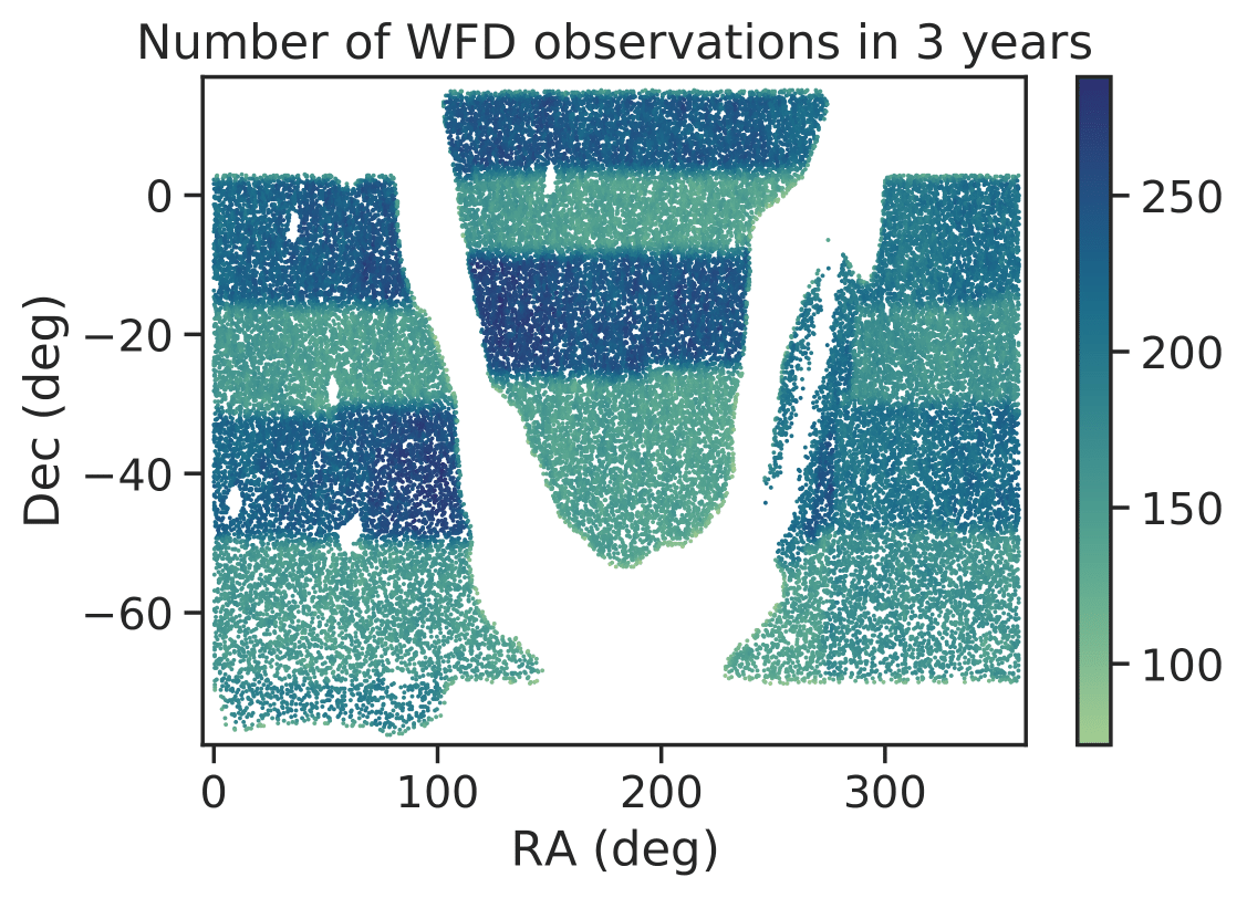
Figure 1: Footprint of the baseline cadence with the number of WFD observations in the first three years ($1.5$ years of non-rolling followed by $1.5$ years of rolling cadence). The dark bands correspond to the ‘active’ area of the rolling cadence which is observed at a higher cadence, and the light bands to the ‘background’.

Table 1: Breakdown of the number of SNe per class and observing strategy used in this work. (Left) events simulated between years $1.5$ and $3$ of the survey. (Right) events simulated between years $0$ and $3$ of the survey.

Y1.5-3 baseline
SN class	$N_{\mathrm{training}}$ ($\%$)	$N_{\mathrm{test}}$ ($\%$)
SN Ia	$1738$ ($64\%$)	$755330$ ($62\%$)
SN Ibc	$231$ ($8\%$)	$57854$ ($5\%$)
SN II	$759$ ($28\%$)	$405139$ ($33\%$)
Total	$2728$ ($100\%$)	$1218323$ ($100\%$)

Y0-3 baseline
SN class	$N_{\mathrm{training}}$ ($\%$)	$N_{\mathrm{test}}$ ($\%$)
SN Ia	$3421$ ($65\%$)	$1563427$ ($62\%$)
SN Ibc	$460$ ($9\%$)	$119703$ ($5\%$)
SN II	$1392$ ($26\%$)	$818241$ ($33\%$)
Total	$5273$ ($100\%$)	$2501371$ ($100\%$)

No-roll
SN class	$N_{\mathrm{training}}$ ($\%$)	$N_{\mathrm{test}}$ ($\%$)
SN Ia	$1787$ ($63\%$)	$875487$ ($63\%$)
SN Ibc	$240$ ($9\%$)	$66389$ ($5\%$)
SN II	$801$ ($28\%$)	$445651$ ($32\%$)
Total	$2828$ ($100\%$)	$1387527$ ($100\%$)

Presto-color
SN class	$N_{\mathrm{training}}$ ($\%$)	$N_{\mathrm{test}}$ ($\%$)
SN Ia	$3243$ ($63\%$)	$1287360$ ($65\%$)
SN Ibc	$483$ ($9\%$)	$93776$ ($5\%$)
SN II	$1422$ ($28\%$)	$597310$ ($30\%$)
Total	$5148$ ($100\%$)	$1978446$ ($100\%$)

A key aim of the new LSST observing strategy simulations is to evaluate whether a rolling cadence is suitable, as demonstrated by science metrics (Ph1R). In this work, we studied the impact of the rolling cadence on the photometric classification of SNe by comparing the baseline observing strategy with a similar strategy without the rolling (noroll_v2.0, hereafter referred to as no-roll). Since the rolling starts in year $1.5$ of the baseline simulation, we restricted this comparative analysis to the events observed between years $1.5$ and $3$ on both simulations. We refer to this subset of the baseline dataset as Y1.5-3 baseline; we used Y0-3 baseline when considering the entire three years. The simulations are otherwise identical.

Another aim of the new observing strategies is to investigate modifications of the intra-night cadence. In this work, we studied the impact of adding a third visit per night in a passband that had been previously observed; this addition is motivated by expected improvements to the performance of early classification and fast transient detection. The presto-color family (Bianco et al., 2018, 2019) encompasses a number of variations of the third visit inclusion, such as different intra-night gaps between the observations (e.g. $1.5$ hrs to $4$ hrs between the first pair of observations and the third), whether the initial pair of visits is in consecutive passbands ($g+r$, $r+i$ or $i+z$) or mixed passbands ($g+i$, $r+z$ or $i+y$), and whether to obtain the visit triplet every night or every other night (Ph1R). SNe do not vary significantly during a single night, so the difference in intra-night gaps between $1.5$ hrs and $4$ hrs has minimal impact. We thus chose a presto-color cadence whose third visit has an intermediate value of $2.5$ hrs for the intra-night gap (presto_gap2.5_mix_v2.0, hereafter referred to as presto-color). Since the total number of visits per pointing is fixed, adopting a presto-color cadence results in longer inter-night gaps; further, each field is observed for fewer nights in total. Similarly to baseline, the rolling starts in year 1.5 of the presto-color cadence; thus we compare baseline and presto-color for the entire first three years of LSST. For more details on the simulations, see Ph1R and the descriptions in the associated Jupyter Notebook.

2.3 Supernovae Models

Following Alves et al. (2022), we focused on classifying SN Ia, SN Ibc, and SN II, which have been found to be difficult transient classes to distinguish (Hložek et al., 2020). We simulated each class in a similar manner to Kessler et al. (2019), using models from Guy et al. (2010); Kessler et al. (2010b, 2013); Villar et al. (2017); Pierel et al. (2018); Guillochon et al. (2018). However, similarly to Lokken et al. (2023), we did not include the SNIbc-MOSFiT model because it produces unphysical light curves. We also adjusted the relative fraction of simulated core-collapse SNe (CC SNe) to follow Table 3 of Shivvers et al. (2017). Additionally, due to the lack of SN IIb models in Kessler et al. (2019), we redistributed their fraction among the other stripped envelope SNe (SN Ib and SN Ic); see Table 2 of Appendix A for the relative rates used to simulate CC SNe in this work. Table 1 shows the resulting number of SNe per class for each observing strategy.

2.4 Framework for Generating Simulations

Our SNe simulations were built on top of the observing strategy cadences produced by FBS previously discussed in Section 2.2 (Naghib et al., 2019); this scheduler decides the passband to use and the direction to point the telescope to using a Markovian Decision Process, while accounting for interruptions, such as telescope maintenance downtime. Despite the FBS outputs containing a record of each simulated pointing of the survey, for generating light curves it is more convenient to compute all the observations of each event, and iterate over the events. Therefore, we used the python package OpSimSummary (Biswas et al., 2020, 2022) to reorder of the observations. This package also translates the FBS output into the appropriate format for use with the SNe simulation code from SNANA (Kessler et al., 2009b), which we used to generate realistic light curves in the LSST passbands. We broadly followed the methodology described in Kessler et al. (2019) which relies on SNANA to generate simulated datasets of SNe and associated metadata (e.g. host galaxy photometric redshift and its uncertainty). SNANA uses models of the SN sources, observing conditions, observing strategy, and instrumental noise to generate light curves. Then, it applies triggers to select the observations that would be seen by LSST. Following Kessler et al. (2019), we applied the SNANA transient trigger to only keep events with at least two detections in our datasets; SNANA uses the DES-SN detection model from Kessler et al. (2015) to decide which observations are flagged as detected. See Figure 13 of Kessler et al. (2019) for a summary of the SNANA simulation stages.

Following Kessler et al. (2019)’s usage of SNANA, we truncated the 10-year survey to the first three years, removed season fragments with less than $30$ days, and used the cosmological parameters $\Omega_{\mathrm{m}}=0.3$, $\Omega_{\Lambda}=0.7$, $w_{0}=-1$, and $H_{0}=70$. However, we used an updated version of the code which included improvements for the K-corrections for events at the highest simulated redshift. We made two further changes from Kessler et al. (2019) to improve the realism of our simulations, as follows. While Kessler et al. (2019) used a pixel-flux saturation of 3,900,000 photoelectrons/pixel, we used the more realistic value of 100,000 photoelectrons/pixel. We also corrected the code to ensure that any observations in the same band in a given night are co-added and count as a single observation. We provide our SNANA input files for each observing strategy simulation on zenodo.

Figure 2: Host galaxy photometric redshift distribution per supernova class for Y0-3 baseline, where SN Ia, SN Ibc, SN II are shown, respectively, on the left, middle and right panels. The training set distribution (solid line) is not representative of the test set (dashed line), but the augmented training set (bold solid line) is close to the desired test distribution.

3 Photometric Classification

We followed the approach of Alves et al. (2022) to photometrically classify the SNe simulated from each observing strategy. In that work, we benchmarked our classification approach against the winning PLAsTiCC entry (Boone, 2019) and showed that our classification results were generalizable; they hold if we replace our classification predictions with the predictions of Boone (2019). Here we used the photometric transient classification library snmachine (Lochner et al., 2016; Alves et al., 2022) and updated it to handle the output files of SNANA (FITS files). In the sections below, we describe the main steps of the approach and any modifications relative to Alves et al. (2022).

3.1 Light Curve Preprocessing

Following Alves et al. (2022), we preprocessed the simulated light curves to only include the observing season in which the SNe is detected. To isolate this season for each event, we removed all observations $50$ days before the first detection and $50$ days after the last. Next, we divided the remainder light curve into sequences of observations without inter-night gaps $>50$ days; we selected our preprocessed light curve as the sequence of observations which contained the largest number of detections. Finally we translated the light curve so the first observation was at time zero. The longest resulting light curves, as measured between the first and last observations, lasted for $274$, $253$, and $295$ days respectively, for baseline, no-roll, and presto-color.

3.2 Gaussian Process Modeling of Light Curves

We used GP regression (e.g. MacKay, 2003; Rasmussen & Williams, 2005) to model each light curve. Following Boone (2019); Alves et al. (2022), we fitted two-dimensional GPs in time and wavelength; we applied a null mean function and a Matérn 3/2 kernel for the GP covariance. We fixed the length-scale of the wavelength dimension to $6000\,\mathring{\mathrm{A}}$ and used maximum likelihood estimation to optimize the time dimension length-scale and amplitude per event. We implemented the GPs with the python package George (Ambikasaran et al., 2014). We note that Stevance & Lee (2022) investigated possible improvements to using GPs for SNe light curve fitting. We leave these extensions to future work on SNe classification.

3.3 Augmentation

We applied the methodology developed in Alves et al. (2022) to augment the training set of each simulated observing strategy to be representative of their respective test set in terms of the photometric redshift distribution per SNe class, the cadence of observations, and the flux uncertainty distribution. We delineate below the departures from the augmentation procedure described in Section 4 of Alves et al. (2022) and refer the details to Appendix B.

We augmented the training set SNe to generate synthetic events at a different redshift from the original; this approach relied on using two-dimensional GP models of the training set events to generate the synthetic light curves. Since we removed a SN model (as mentioned in Section 2.3), the redshift distribution of the events changed with respect to Alves et al. (2022). Consequently, we used a different distribution to produce the augmented training sets, as detailed in Appendix B.

Following our previous work, we generated $15440$ WFD synthetic events for each SNe class. Figure 2 shows that for the Y0-3 baseline, the photometric redshift distribution of the augmented training set is closer to the test set than the original training set. Although the distribution does not match exactly, it is sufficiently close to expect minimal impact on performance. Ensuring identical distributions could require introducing an undesirable amount of fine-tuning to the methodology, and hence we have not attempted to obtain a closer match. Comparable figures for the other observing strategies are shown in Figure 14 of Appendix B.

We also tuned the distribution of the number of observations and their flux uncertainty for the synthetic events of each observing strategy. We drew the target number of observations for each light curve from a Gaussian mixture model based on the test set; Table 3 of Appendix B shows the parameters used for each observing strategy. For the flux uncertainty, we followed Boone (2019); Alves et al. (2022) and combined the uncertainty predicted by the GP in quadrature with a value drawn from the flux uncertainty distribution of the test set. Table 4 of Appendix B shows the parameters of the Gaussian mixture model used to fit the flux uncertainty distribution of each passband and observing strategy.

3.4 Feature Extraction

For photometric classification we used the host galaxy photometric redshift, its uncertainty, and model-independent wavelet coefficients obtained from the GP fits as features. The redshift features mentioned above were directly obtained from the metadata associated with each event. For the wavelet features, we followed the feature extraction procedure of Lochner et al. (2016); Alves et al. (2022), which we briefly summarize in the following paragraph.

To perform a wavelet decomposition on the light curves we sampled them onto a time grid. We used the two-dimensional GP that models each light curve to interpolate between the observations. For uniformity, we used the same time grid for all the observing strategies; the time range of the grid corresponds to the maximum light curve duration of the events, $295$ days. Following Alves et al. (2022) we chose $292$ grid points to sample the events approximately once per day. Next, we performed a two-level wavelet decomposition using a Stationary Wavelet Transform and the symlet family of wavelets. These decomposition choices resulted in $7008$ redundant wavelet coefficients per event. Following Lochner et al. (2016); Alves et al. (2022), we reduced the dimensionality of the wavelet space to $40$ components using Principal Component Analysis (PCA; Pearson, 1901; Hotelling, 1933). We used the augmented training set of each observing strategy to construct the dimensionality-reduced wavelet space; the test set events were projected onto the corresponding wavelet space.

3.5 Classification

We used snmachine to build a photometric classifier trained on the augmented training set. We used Gradient Boosting Decision Trees (GBDT) (Friedman, 2002), classifiers whose predictions are based on ensembles of decision trees. We trained the classifier for each observing strategy separately, using dedicated augmented training sets (Section 3.3) and features (Section 3.4). The GBDT classifier hyperparameters were optimized following the procedure described in Section 3.4 of Alves et al. (2022); Table 5 of Appendix B shows the values of the hyperparameters per observing strategy.

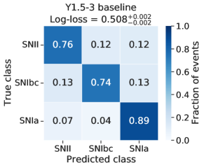
Figure 3: Normalized test-set confusion matrix for the classifier trained on the augmented training set of the Y1.5-3 baseline (left panel) and the no-roll cadences (right panel). The uncertainty in the log-loss corresponds to the $95\%$ confidence intervals obtained by bootstrapping. The results show a slightly higher SNe classification performance when rolling is implemented at the level in the baseline cadence.

3.5.1 Performance Evaluation

We used the PLAsTiCC weighted log-loss metric (The PLAsTiCC team et al., 2018; Malz et al., 2019) to optimize the photometric classifiers and to evaluate their performance. Following the PLAsTiCC challenge, we gave the same weight to each SN class.

Confusion matrices are commonly used to assess the performance of classifiers (see e.g. Hložek et al., 2020). To produce a confusion matrix, we first assigned each test set event to its most probable class. For ease of comparison between different classes and observing strategies, we normalized the resulting confusion matrices by dividing each entry by the true number of SNe in each class. In this setting, a perfect classification results in the identity matrix.

We measured the classification performance using the recall (also called completeness/sensitivity) and precision of each SNe class. These are defined as

$$\mathrm{recall}=\dfrac{\mathrm{TP}}{\mathrm{TP}+\mathrm{FN}}$$ (1)

and

$$\mathrm{precision}=\dfrac{\mathrm{TP}}{\mathrm{TP}+\mathrm{FP}}\,,$$ (2)

where in a binary classification setting, TP, FN, and FP are, respectively, the number of true positives, false negatives and false positives.

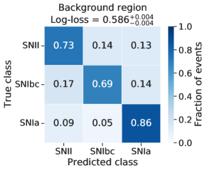
Figure 4: Normalized test-set confusion matrices for the classifier trained on the augmented training set of the Y1.5-3 baseline cadence. The left panel shows the results for the active region of the rolling cadence and the right panel for the background region. The uncertainty in the log-loss corresponds to the $95\%$ confidence intervals obtained by bootstrapping. The results show a significantly higher SNe classification performance for the active region of the rolling cadence.

The computational performance of this procedure and an estimate of the resources needed for reproducing this analysis are discussed in Appendix C.

4 Results and Implications for Observing Strategy

Here we present our results on the impact of rolling cadence and the intra-night gap on SNe classification performance. We perform a comparative analysis for these two cases relative to the baseline strategy in Section 4.1. In our previous work (Alves et al., 2022) we found that light curve length (time difference between the first and last observation after the light curve preprocessing described in Section 3.1) and inter-night gap (time difference between consecutive observations which are more than $12$ hrs apart) were the key properties of observing strategies affecting classification performance. We thus investigate how the no-roll and presto-color families affect the recall and precision as a function of several factors including the above.

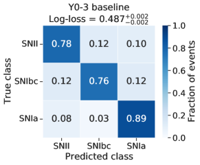
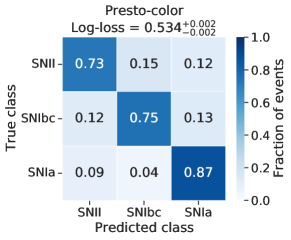
Figure 5: Normalized test-set confusion matrix for the classifier trained on the augmented training set of the Y0-3 baseline (left panel) and the presto-color cadences (right panel). The uncertainty in the log-loss corresponds to the $95\%$ confidence intervals obtained by bootstrapping. The results show that visiting each event twice per night (baseline cadence) instead of three times yields a $\sim 10$% higher SNe classification performance.

4.1 Overall Classification Performance

Figure 3 shows the confusion matrices for classifiers trained on the augmented training set of Y1.5-3 baseline and no-roll. The Y1.5-3 baseline classifier yields a slightly higher performance for SN Ibc, SN II, and a percent-level improvement in the PLAsTiCC log-loss metric. This small difference indicates that rolling at this level makes a negligible difference to the overall efficacy of SNe photometric classification. However this result masks a significant difference between the classification efficacy between the active and background regions due to an averaging effect. Therefore we also investigated the difference in performance between the active region (which we visually identified as the dark bands in Fig. 1; 65% of the test set events) and the background region (35% of the test set events). The confusion matrices in Fig. 4 show that the classification performance of the active region is higher than of the background region for all SNe classes. Indeed the log-loss metric improves by 25% for events in the active region as compared to the background.

Figure 5 shows the confusion matrices for Y0-3 baseline and presto-color. The baseline cadence outperforms presto-color for SN Ia, SN II; the PLAsTiCC log-loss metric degrades by $\sim 10$% for presto-color. While adding a third visit per night is expected to improve performance for early classification and for fast transient detection, our results indicate that this choice moderately degrades classification performance for long-lived transients.

All the observing strategies considered in this work yield a higher performance in terms of the log-loss metric compared with the observing strategy used for PLAsTiCC (Alves et al. 2022 reported a log-loss metric of $0.550$ for this case). This indicates substantial performance gains achieved by recent updates to the FBS scheduler.

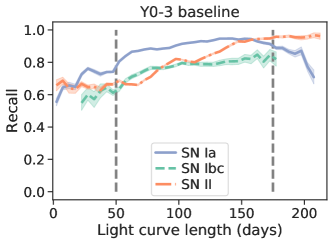
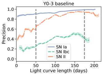
Figure 6: Test-set recall (left panel) and precision (right panel) as a function of light curve length per SNe class for Y0-3 baseline. The shaded areas correspond to the 95% confidence limits obtained by bootstrapping the recall and precision values for each bin. The dashed lines mark the high performance region between $50$ and $175$ days. To remove small-number effects we only present the results for bins with more than $300$ events.

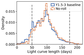
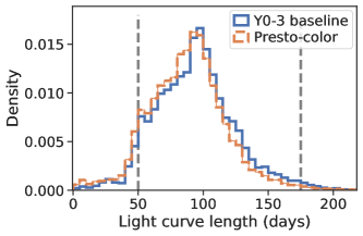
Figure 7: Test-set density of events as a function of light curve length for Y1.5-3 baseline vs no-roll (left panel), and Y0-3 baseline vs presto-color (right panel). The dashed lines mark the high performance region between $50$ and $175$ days.

4.2 Light Curve Length

We found in Alves et al. (2022) that the light curve length of an event has a significant impact on classification performance for long-lived transients such as SNe. In particular, longer light curves are easier to distinguish within a classifier since they incorporate more information about the time evolution of the event. In that work, we focused on events with light curve length between $50$ and $175$ days due to their higher performance. As shown in Figure 6, our results for the Y0-3 baseline show a similar performance behavior. We also find that these conclusions generalize to the other observing strategies analyzed here, and hence the conclusions of Alves et al. (2022) carry over to these new cadence simulations. We note that the recall and precision figures (Figure 6 and subsequent figures) show a small scatter above our statistical uncertainties, likely arising from the limited diversity of the simulations in those particular bins. Figure 7 shows that the distribution of light curve lengths is similar for all the cadences. Indeed the cadence choices currently under consideration (v2.0) have similar distributions of gaps larger than $50$ days, so the light curve length distribution correlates more with the intrinsic duration of the events and our preprocessing of the light curves than with the cadences. Therefore, even though this is a very important factor for overall classification performance, it is not strongly affected by observing strategy choices.

4.3 Median Inter-night Gaps

The observing strategies proposed for LSST have different intra- and inter-night gaps distributions. Given the finite total number of observations available, these distributions are intrinsically linked. In Alves et al. (2022) we demonstrated that the median inter-night gap was a crucial factor in photometric SNe classification, and Ph1R has highlighted the necessity for science-motivated metrics to measure the impact of intra-night gaps. Since the timescale for changes in SN light curves is in days, multiple observations in a single night in the same filter do not contribute towards characterization of the light curve. Here we firstly investigate the impact of a higher intra-night cadence on the median inter-night gap, and hence classification performance.

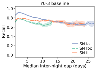
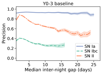
Figure 8: Test-set recall (left panel) and precision (right panel) as a function of inter-night gap per SNe class for Y0-3 baseline. The shaded areas correspond to the 95% confidence limits obtained by bootstrapping the recall and precision values for each bin. To remove small-number effects we only present the results for bins with more than $300$ events.

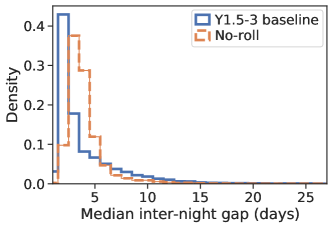
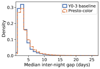
Figure 9: Test-set density of events as a function of inter-night gap for Y1.5-3 baseline vs no-roll (left panel), and Y0-3 baseline vs presto-color (right panel).

Figure 8 shows that, in accordance with our expectations, a lower median inter-night gap leads to higher precision and recall for Y0-3 baseline. SN II show a larger sensitivity to cadence as compared to the other types because SN Ia with high median inter-night gaps are misclassified as SN II, driving down the precision of the latter. Overall, we find similar results for the other observing strategies analyzed.

While this overall conclusion still holds, our results show that the classification performance depends less on the median inter-night gap for this set of observing strategy simulations compared to Alves et al. (2022), where we recommended a median inter-night gap of $\lesssim 3.5$ days. Our new results suggest a cut of $\lesssim 5.5$ days; however, all the current observing strategies aim for a lower median inter-night gap, making such a recommendation redundant. We attribute this reduced sensitivity of classification results to cadence to the recent improvements made to the FBS scheduler.

The left panel of Figure 9 shows that the peak of the median inter-night gap for Y1.5-3 baseline is lower than for no-roll. However, while rolling improves the cadence of the events in the active region, the events in the background region are less regularly sampled than no-roll, which leads to the heavier tail of Y1.5-3 baseline. Thus overall, the classification performance is not significantly improved by rolling.

Since the total exposure time is fixed, the addition of a third visit each night leads to the presto-color events being visited fewer nights. Consequently, this cadence has sparser observations than the Y0-3 baseline. This is reflected in a slightly higher median inter-night gap for presto-color, as shown in the right panel of Figure 9. However, the small shift in the median inter-night gap distribution does not explain the degradation in performance seen for presto-color. We now turn to other cadence properties in order to understand this result.

4.4 Regularity of sampling

In this section we investigate whether the performance differences seen for the cadences considered arise from the (ir)regularity of sampling. Characteristics of the regularity of sampling which are potentially important for classification include large gaps in the light curve and the number of observations near the peak.

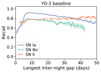
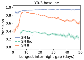
Figure 10: Test-set recall (left panel) and precision (right panel) as a function of the length of the longest inter-night gap per SNe class for Y0-3 baseline. The shaded areas correspond to the 95% confidence limits obtained by bootstrapping the recall and precision values for each bin. To remove small-number effects we only present the results for bins with more than $300$ events. The reduced performance below 8 days corresponds to less than $5\%$ of the events which tend to have very short light curves and therefore are not well classified.

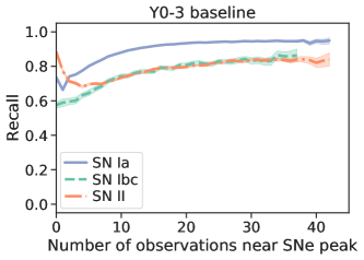
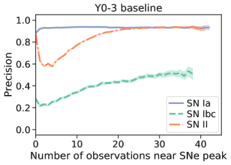
Figure 11: Test-set recall (left panel) and precision (right panel) as a function of number of observations near peak per SNe class for Y0-3 baseline. The shaded areas correspond to the 95% confidence limits obtained by bootstrapping the recall and precision values for each bin. To remove small-number effects we only present the results for bins with more than $300$ events.

In Alves et al. (2022) we found that the GPs successfully interpolate between large gaps ($>10$ days) so the classifier is still able to identify the SNe. Figure 10 confirms that the recall and precision of SNe either slowly decrease or remain constant with the increase of the length of longest inter-night gap. These conclusions also generalize to the other cadences we study. This indicates that the GP step is generally able to interpolate large gaps.

A related consideration for characterizing the regularity of light-curve sampling is observing SNe near peak brightness, where the shape of the light curve changes rapidly. These observations are critical for obtaining a reliable cosmological distance modulus and facilitates accurate photometric classification. In this work, we estimate the SNe peak as the moment that maximizes the GP fit predicted flux in any passband. Then, we define the number of observations near the peak as those $10$ days before and $30$ days after peak brightness; we sum the observations in all passbands to calculate this quantity. Similarly to Alves et al. (2022), we find that the classification performance generally increases with the number of observations near the peak for all the new observing strategies. Figure 11 shows the results for Y0-3 baseline as a representative example. For type Ia SNe, this performance levels off around 15 observations near the peak. This is comparable to the SNe cosmology metric used in Lochner et al. (2022) which requires 5 observations before peak and 10 observations after.

Figure 11 also shows a drop in performance for $\sim 2$ observations near the peak. We find that such events generally only contain the latter part of the transient, and their light curves tend to be flat. The classifier predicts events with flat GP fits as SNe II: the latter tend to have long light curves so it is likely that a flat part of the light curve will be observed. Once there are more observations near the peak, the light curves are not as flat so the SN II recall decreases until there is sufficient information in the light curve for the classifier to correctly identify the transient shape.

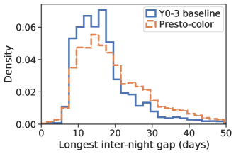
Figure 12: Test-set density of events as a function of the length of the longest inter-night gap for Y1.5-3 baseline vs no-roll (left panel), and Y0-3 baseline vs presto-color (right panel).

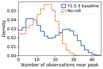
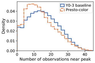
Figure 13: Test-set density of events as a function of number of observations near peak for Y1.5-3 baseline vs no-roll (left panel), and Y0-3 baseline vs presto-color (right panel).

Having established the influence of these characteristics on classification performance, we now consider how they impact the relative classification performance seen in Figures 3 and 5 for the observing strategies considered.

The distribution of the longest inter-night gap in Y1.5-3 baseline exhibits two peaks, as shown in the left panel of Figure 12. This is due to the fact that different areas of the sky start rolling at different times, and Y1.5-3 baseline therefore includes some events in areas of the sky which have not yet started rolling. Thus, we see a second peak at higher values of longest inter-night gap for Y1.5-3 baseline. The peak in the distribution corresponding to the rolling region is at shorter timescales than in no-roll. Overall, these differences do not result in a significant change in performance, because there is no significant tail produced towards longer gaps. By contrast, the right panel of Figure 12 shows that, as expected, the distribution of the longest gaps for presto-color does exhibit a broad tail, due to the more irregular sampling: presto-color has 15% more events which have a long gap of 20 days or more.

Figure 13 compares the distributions of the number of observations near the SNe peak for the various cadences. The left panel of Figure 13 shows the impact of rolling (Y1.5-3 baseline), with a bimodal distribution corresponding to the ‘background’ and ‘active’ areas. While the difference between this distribution and that of no-roll may appear visually large, the latter only has 5% more events in the poorly-classified region ($<15$ observations near peak). This again results in very little difference in classification performance due to rolling. The right panel of Figure 13 shows that presto-color events have $\sim 10$% more events with $<15$ observations near peak compared to Y0-3 baseline. While this difference does not make a large visual impact, it is nevertheless in a regime which strongly affects classification performance.

Figure 5 shows that presto-color mainly impacts classification of type II SNe. In turn, Figure 11 shows that type II SNe classification performance is a strong function of number of observations near peak as compared to the other classes, for $<15$ observations near peak. Since presto-color has more events in this regime, one may therefore expect that SNII classification is particularly degraded for this cadence, and this expectation is confirmed by our results.

Overall, presto-color exhibits small but significant changes in the distribution of the longest inter-night gap and the number of observations near the peak. These combine to result in irregularly-sampled light curves, which in turn leads to degraded classification performance.

5 Discussion and Conclusions

We have presented the impact of LSST cadence choices on the performance of SNe photometric classification, using simulated multi-band light curves from the LSST baseline cadence, the non-rolling cadence, and a presto-color cadence. For each dataset considered, we augmented the non-representative training set to be representative of the test set and built a classifier using the photometric transient classification library snmachine. In line with previous studies, we confirmed that the light curve length, median inter-night gap and number of observations near the SNe peak, which differ between the cadences, affect the photometric classification.

Previous works argued that a rolling cadence benefits SNe science due to the improved sampling but that more in-depth simulations and studies were needed (LSST Science Collaboration et al., 2017; Lochner et al., 2018). We find that the considered rolling cadence (which increases by $90\%$ the footprint weight of the active region) only mildly improves the overall classification performance. However, crucially, our results show that the active region of the rolling cadence as implemented in the current baseline strategy has a significantly higher classification performance than the background region. This in turn suggests that the SN Ia light curves in the active region could be better measured, and hence more useful for cosmological analyses. We now investigate this point.

Lochner et al. (2022) defines a set of light curve requirements for well-measured SN Ia which form the basis of seven cosmology metrics; in Appendix D we present the updated version of these requirements currently being used by LSST DESC. Considering all but one of the updated requirements (ignoring a color-related requirement due to its computationally-intensive nature), we compared the SN Ia light-curves in the active and background regions of the Y1.5-3 baseline. We found that $\sim 50\%$ of the SN Ia in the active region fulfilled the light curve requirements, compared with only $\sim 20\%$ of the SN Ia in the background region. While these results are indicative rather than definitive due to ignoring the color requirement, they suggest that the 25% improvement in the classification performance log-loss metric in the active region is also associated with an increase of up to a factor of $2.7$ in the number of cosmologically-useful SN Ia in the active region. These results taken together strongly motivate the implementation of a rolling cadence within the baseline observing strategy.

We also found that the presto-color cadence led to shorter and sparser light curves: the light curve length distribution of this cadence on Figure 7 is skewed towards lower values. Additionally, there are more presto-color events with large gaps and fewer observations near the SNe peak. These results indicate that the events simulated under this cadence have a more heterogeneous sampling than the baseline events. Irregular sampling, especially around the peak where the light curve varies more rapidly, results in worse constraints on its shape; therefore the classifier is less able to distinguish between the SNe classes.

Since the third visit per night implemented in presto-color is in part motivated by facilitating early transient classification, our results imply that there is a trade-off in the observing strategy requirements of early and full light-curve classification.

The accuracy of SN Ia photometric classification and core-collapse contamination affect the measurements of the dark energy equation of state parameter (Kessler & Scolnic, 2017; Jones et al., 2017). While a Bayesian methodology can marginalize over the contamination, minimizing such contamination reduces systematic uncertainties in cosmological constraints (Kunz et al., 2007; Lochner et al., 2013; Roberts et al., 2017; Jones et al., 2018). Since SNe cosmology with LSST is expected to be limited by systematic uncertainties, the relationship between the efficacy of photometric classification and cosmological constraints is of crucial importance.

We expect these conclusions to be general and hold for different photometric classifiers that rely on the full light curve, as shown in Alves et al. (2022). In the future, we plan to develop a fast proxy metric to evaluate the impact of cadence choices on photometric classification directly on the observing strategy cadences produced by the FBS (Naghib et al., 2019), avoiding the time-consuming SNe simulations and classification steps that were necessary in this work. More broadly, our results contribute to the pioneering process of community-focussed experimental design and optimization of the LSST observing strategy.

Appendix A Simulated CC SN rates

In this appendix we present the absolute and relative rates used to simulate CC SNe in this work. These rates follow Shivvers et al. (2017) with the adjustments described in Section 2.4. Table 2 includes both the rates of each CC SNe class and the models used (see Kessler et al. (2019) for further details). The resulting number of SNe for each class is shown in Table 1.

Table 2: Absolute and relative scale rate used to simulate core-collapse SNe in this work expressed in percentage. The rates follow Shivvers et al. (2017) and the SNe models are described in Kessler et al. (2019); SNIb-Templates and SNIc-Templates are both described together as SNIbc-Templates.

Subtypes	Model name	Abs. scale rate (rel. scale rate) %
Core-collapse
II	see Hydrogen Rich	$69.6$ ($100$)
Ib+Ic	see Stripped Envelope	$30.4$ ($100$)
Hydrogen Rich - class SN II
II (IIP, IIL)	SNII-NMF	$32.45$ ($23.325$)	$64.9$ ($93.3$)
	SNII-Templates	$32.45$ ($23.325$)
IIn	SNIIn-MOSFiT	$4.7$ ($3.35$)	$4.7$ ($6.7$)
Stripped Envelope - class SN Ibc
Ib	SNIb-Templates	$5.4$ ($17.8$)	$10.8$ ($35.6$)
Ic	SNIc-Templates	$3.75$ ($12.35$)	$7.5$ ($24.7$)

Appendix B Augmentation details and Classification Hyperparameters

Section 3.3 described the differences between the augmentation procedure used in this work and the one in the Section 4 of Alves et al. (2022). In particular, we changed the distribution used to create the augmented training sets because the removal of the SNIbc-MOSFiT model (mentioned in Section 2.3) altered the redshift distribution of the events. In this work, we augmented each event between the redshift limits $z_{\mathrm{min}}$ and $z_{\mathrm{max}}$ from Section 4.2 of Alves et al. (2022):

$$\begin{aligned} z_{\mathrm{min}}&\approx\max\left\{0,0.90\,z_{\mathrm{ori}}-0.10\right\}\,\text{and}\\ z_{\mathrm{max}}&\approx 1.43\,z_{\mathrm{ori}}+0.43\,,\end{aligned}\,$$ (B1)

where $z_{\mathrm{ori}}$ is the spectroscopic redshift of the original event. However, we used a different class-agnostic target distribution. In particular, we drew an auxiliary value $z^{*}$ from a log-trapezoidal distribution; the probability density function of the trapezoid distribution is

$$f\left(x\right)=\begin{cases}\dfrac{2}{\Delta x}\left[\dfrac{x_{\mathrm{max}}-0.8x}{\Delta x}-0.1\right]&x\in\left[x_{\mathrm{min}},x_{\mathrm{max}}\right]\\ 0&\text{otherwise}\end{cases}\,,$$ (B2)

where $x_{\mathrm{min}}=\log\left(z_{\mathrm{min}}\right)$, $x_{\mathrm{max}}=\log\left(z_{\mathrm{max}}\right)$, and ${\Delta x=x_{\mathrm{max}}-x_{\mathrm{min}}}$. Then, we calculated the redshift of the new augmented event following Alves et al. (2022), ${z_{\mathrm{aug}}\left(z^{*}\right)=-z^{*}+z_{\mathrm{min}}+z_{\mathrm{max}}}$.

For each observing strategy, we also adjusted the parameters of the Gaussian mixture models used to fit the number of observations per light curve (Table 3) and the flux uncertainty distribution of each passband (Table 4). We fitted Gaussian mixture models to the test set, and used visual inspection to select the number components. The resulting photometric distributions are shown in Figure 14.

In this section we also show the hyperparameters values of the GBDT classifier used for each observing strategy (Table 5).

Table 3: Parameters of Gaussian mixture models used to fit the number of observations of the test set light curves for each observing strategy. These values were later used to create an augmented training set (Section 3.3). We used visual inspection to select the number components of the Gaussian mixture models; that number is indicated through the number of weights provided for each observing strategy. The weight, mean and variance of each component are displayed in the same order.

	Y1.5-3 baseline	No-roll
weights	$[0.322,0.678]$	$[0.289,0.215,0.181,0.315]$
means	$[16.86,61.15]$	$\left[31.93,18.07,59.65,45.35\right]$
variances	$[46.62,561.06]$	$\left[30.23,42.76,75.83,34.96\right]$
	Y0-3 baseline	Presto-color
weights	$\left[0.679,0.321\right]$	$\left[0.626,0.374\right]$
means	$\left[33.6,65.1\right]$	$\left[27.11,53.72\right]$
variances	$\left[199.09,453.67\right]$	$\left[125.04,252.05\right]$

Table 4: Parameters of Gaussian mixture models used to fit the flux uncertainty distribution of the test set in each passband (ugrizy) and observing strategy. These values were later used to create an augmented training set (Section 3.3). We used visual inspection to select the number components of the Gaussian mixture models; that number is indicated through the number of weights provided for each observing strategy. The weight, mean and variance of each component are displayed in the same order.

		Y1.5-3	No-roll	Y0-3	Presto-color
		baseline		baseline
u	weights	$[0.24,0.76]$	$[0.25,0.75]$	$[0.29,0.71]$	$[0.64,0.36]$
	means	$[2.34,1.92]$	$[2.29,1.95]$	$[2.24,1.93]$	$[1.96,2.35]$
	variances	$[0.46,0.10]$	$[0.45,0.10]$	$[0.38,0.09]$	$[0.09,0.28]$
g	weights	$[0.88,0.12]$	$[0.11,0.89]$	$[0.88,0.12]$	$[0.10,0.90]$
	means	$[1.26,2.06]$	$[2.13,1.27]$	$[1.26,1.98]$	$[2.12,1.41]$
	variances	$[0.11,0.93]$	$[1.08,0.12]$	$[0.11,0.85]$	$[0.98,0.14]$
r	weights	$[0.27,0.73]$	$[0.76,0.24]$	$[0.29,0.71]$	$[0.23,0.45,0.32]$
	means	$[1.92,1.57]$	$[1.59,1.92]$	$[1.89,1.58]$	$[2.82,1.60,2.20]$
	variances	$[0.38,0.09]$	$[0.09,0.40]$	$[0.34,0.08]$	$[0.30,0.08,0.12]$
i	weights	$[0.62,0.38]$	$[0.63,0.37]$	$[0.63,0.37]$	$[0.66,0.34]$
	means	$[1.97,2.45]$	$[1.98,2.44]$	$[1.99,2.45]$	$[1.96,2.48]$
	variances	$[0.08,0.22]$	$[0.08,0.23]$	$[0.08,0.20]$	$[0.10,0.26]$
z	weights	$[1.]$	$[1.]$	$[1.]$	$[1.]$
	means	$[2.65]$	$[2.65]$	$[2.67]$	$[2.68]$
	variances	$[0.14]$	$[0.14]$	$[0.14]$	$[0.17]$
y	weights	$[1.]$	$[1.]$	$[1.]$	$[0.62,0.38]$
	means	$[3.23]$	$[3.22]$	$[3.23]$	$[3.07,3.52]$
	variances	$[0.15]$	$[0.14]$	$[0.14]$	$[0.07,0.13]$

Y1.5-3 baseline

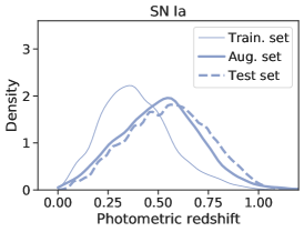
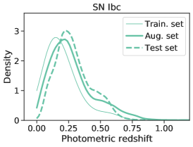
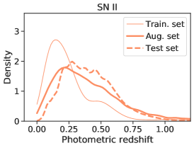
No-roll

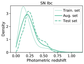
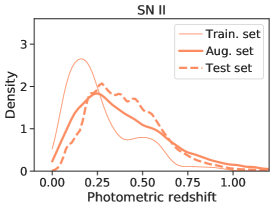
Y0-3 baseline

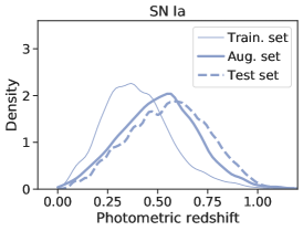
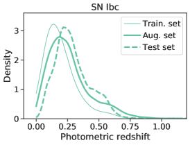
Presto-color

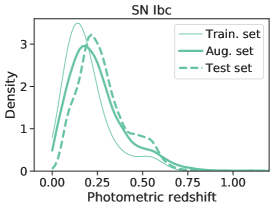
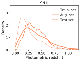
Figure 14: Host galaxy photometric redshift distribution per supernova class, where SN Ia, SN Ibc, SN II are shown, respectively, on the left, middle and right panels. Each row shows the training (solid line), augmented training (bold solid line) and test set distributions (dashed line) for each observing strategy. For all the observing strategies, the augmented training set distribution is closer to the test set than the original training set.

Table 5: Values of the optimized LightGBM model hyper-parameters used in each observing strategy. The hyper-parameters are described in the library documentation.

Hyper-parameter name	Y1.5-3 baseline	No-roll	Y0-3 baseline	Presto-color
boosting_type	gbdt	gbdt	gbdt	gbdt
learning_rate	$0.14$	$0.14$	$0.16$	$0.18$
max_depth	$19$	$19$	$13$	$19$
min_child_samples	$70$	$70$	$70$	$70$
min_split_gain	$0.6$	$0.0$	$0.1$	$0.0$
n_estimators	$115$	$115$	$115$	$115$
num_leaves	$50$	$50$	$55$	$50$

Appendix C Computational Resources

We simulated the observing strategy datasets on a Intel E5-2680v4 @ 2.4 GHz. Each dataset with $2.5\times 10^{6}$ events takes $\sim 200$ core hours to simulate. The data processing, classification and analysis was performed on an Intel(R) Xeon(R) CPU E5-2697 v2 (2.70GHz). Using a single core, the pipeline takes $\sim 5.6$ hrs to preprocess these events. Modeling them with GPs and performing their wavelet decomposition takes $\sim 44.4$ hrs. Generating a augmented training set with $15440$ events takes $\sim 9$ hrs, and reducing the dimensionality of their wavelet features using PCA takes $\sim 45$ min. Optimizing the GBDT classifier takes $\sim 5.5$ hrs. Obtaining the test set predictions on the pre-computed test set features with the trained classifier takes $5$ min. Overall, the entire classification pipeline takes $\sim 200+70$ core hours of computing time for each observing strategy.

Appendix D Well-measured Type Ia Supernovae

To measure cosmological parameters accurately, it is crucial to obtain a large sample of well-measured SN Ia. Lochner et al. (2022) presented a set of requirements to denote a SN Ia light curve as well-measured; these requirements have recently been updated and refined. The updated requirements only use the light curve observations in the $grizy$ passbands which have signal-to-noise ratio $>1$, and which satisfy

$$380\,\text{nm}<\dfrac{\bar{\lambda}_{\text{obs}}}{1+z}<700\,\text{nm}\,,$$ (D1)

where $\bar{\lambda}_{\text{obs}}$ is the mean wavelength of the telescope in the passband of the considered observation. They also limit the light curves to the observations with phases between $20$ days before and $60$ days after peak; the phase of the light curve is given by

$$\dfrac{t-t_{\text{peak}}}{1+z}\,,$$ (D2)

where $t$ is the time of the observation and $t_{\text{peak}}$ is the time of the SNe peak brightness. The requirements are:

• at least 3 observations before peak with phase $>-20$

• at least 8 observations after peak with phase $<60$

• at least 1 observation with phase $\leq 10$

• at least 1 observation with phase $\geq 20$

• $\sigma_{C}<0.04$, where $\sigma_{C}$ is color uncertainty obtained when fitting the light curve with the SALT2 package (Guy et al., 2007).

In this work we ignore the last requirement because SALT2 fits are computationally intensive. We also use the light curves preprocessed as described in Section 3.1 rather than the three-year-long light curves.

References

- Abbott et al. (2019) Abbott, T. M. C., Allam, S., Andersen, P., et al. 2019, The Astrophysical Journal, 872, L30, doi: 10.3847/2041-8213/ab04fa
- Allam Jr. & McEwen (2021) Allam Jr., T., & McEwen, J. D. 2021, arXiv preprint arXiv:2105.06178, doi: 10.48550/arXiv.2105.06178
- Alves et al. (2022) Alves, C. S., Peiris, H. V., Lochner, M., et al. 2022, The Astrophysical Journal Supplement Series, 258, 23, doi: 10.3847/1538-4365/ac3479
- Ambikasaran et al. (2014) Ambikasaran, S., Foreman-Mackey, D., Greengard, L., Hogg, D. W., & O’Neil, M. 2014, arXiv preprint arXiv:1403.6015v2, doi: 10.48550/arXiv.1403.6015
- Astier et al. (2006) Astier, P., Guy, J., Regnault, N., et al. 2006, Astronomy & Astrophysics, 447, 31, doi: 10.1051/0004-6361:20054185
- Astropy Collaboration et al. (2013) Astropy Collaboration, Robitaille, T. P., Tollerud, E. J., et al. 2013, Astronomy & Astrophysics, 558, A33, doi: 10.1051/0004-6361/201322068
- Astropy Collaboration et al. (2018) Astropy Collaboration, Price-Whelan, A. M., Sipőcz, B. M., et al. 2018, The Astronomical Journal, 156, 123, doi: 10.3847/1538-3881/aabc4f
- Barbier et al. (2016) Barbier, J., Dia, M., Macris, N., et al. 2016, in Advances in Neural Information Processing Systems, ed. D. Lee, M. Sugiyama, U. Luxburg, I. Guyon, & R. Garnett, Vol. 29 (Curran Associates, Inc.). https://proceedings.neurips.cc/paper/2016/file/621bf66ddb7c962aa0d22ac97d69b793-Paper.pdf
- Betoule et al. (2014) Betoule, M., Kessler, R., Guy, J., et al. 2014, Astronomy & Astrophysics, 568, A22, doi: 10.1051/0004-6361/201423413
- Bianco et al. (2018) Bianco, F. B., Graham, M., Drout, M. R., et al. 2018, Presto-Color: An LSST Cadence for Explosive Physics & Fast Transients, White paper
- Bianco et al. (2019) Bianco, F. B., Drout, M. R., Graham, M. L., et al. 2019, Publications of the Astronomical Society of the Pacific, 131, 068002, doi: 10.1088/1538-3873/ab121a
- Biswas et al. (2022) Biswas, R., Alves, C., Setzer, C., Frohmaier, C., & Azfar, F. 2022, LSSTDESC/OpSimSummary: 3.0.0, Zenodo, doi: 10.5281/ZENODO.6350796
- Biswas et al. (2020) Biswas, R., Daniel, S. F., Hložek, R., Kim, A. G., & and, P. Y. 2020, The Astrophysical Journal Supplement Series, 247, 60, doi: 10.3847/1538-4365/ab72f2
- Boone (2019) Boone, K. 2019, The Astronomical Journal, 158, 257, doi: 10.3847/1538-3881/ab5182
- Boone (2021) —. 2021, The Astronomical Journal, 162, 275, doi: 10.3847/1538-3881/ac2a2d
- Brout et al. (2022) Brout, D., Scolnic, D., Popovic, B., et al. 2022, The Astrophysical Journal, 938, 110, doi: 10.3847/1538-4357/ac8e04
- Carrick et al. (2021) Carrick, J. E., Hook, I. M., Swann, E., et al. 2021, Monthly Notices of the Royal Astronomical Society, 508, 1, doi: 10.1093/mnras/stab2343
- Caswell et al. (2020) Caswell, T. A., Droettboom, M., Lee, A., et al. 2020, matplotlib/matplotlib: REL: v3.3.2, Zenodo, doi: 10.5281/ZENODO.4030140
- Charnock & Moss (2017) Charnock, T., & Moss, A. 2017, The Astrophysical Journal, 837, L28, doi: 10.3847/2041-8213/aa603d
- Friedman (2002) Friedman, J. H. 2002, Computational Statistics & Data Analysis, 38, 367, doi: 10.1016/s0167-9473(01)00065-2
- Gonzalez et al. (2018) Gonzalez, O. A., Clarkson, W., Debattista, V. P., et al. 2018, arXiv preprint arXiv:1812.08670, doi: 10.48550/arXiv.1812.08670
- Guillochon et al. (2018) Guillochon, J., Nicholl, M., Villar, V. A., et al. 2018, The Astrophysical Journal Supplement Series, 236, 6, doi: 10.3847/1538-4365/aab761
- Guy et al. (2007) Guy, J., Astier, P., Baumont, S., et al. 2007, Astronomy & Astrophysics, 466, 11, doi: 10.1051/0004-6361:20066930
- Guy et al. (2010) Guy, J., Sullivan, M., Conley, A., et al. 2010, Astronomy & Astrophysics, 523, A7, doi: 10.1051/0004-6361/201014468
- Harris et al. (2020) Harris, C. R., Millman, K. J., van der Walt, S. J., et al. 2020, Nature, 585, 357, doi: 10.1038/s41586-020-2649-2
- Hložek et al. (2020) Hložek, R., Ponder, K. A., Malz, A. I., et al. 2020, arXiv preprint arXiv:2012.12392, doi: 10.48550/arXiv.2012.12392
- Hotelling (1933) Hotelling, H. 1933, Journal of Educational Psychology, 24, 417, doi: 10.1037/h0071325
- Hunter (2007) Hunter, J. D. 2007, Computing in Science & Engineering, 9, 90, doi: 10.1109/MCSE.2007.55
- Ivezić et al. (2019) Ivezić, Ž., Kahn, S. M., Tyson, J. A., et al. 2019, The Astrophysical Journal, 873, 111, doi: 10.3847/1538-4357/ab042c
- Jones et al. (2017) Jones, D. O., Scolnic, D. M., Riess, A. G., et al. 2017, The Astrophysical Journal, 843, 6, doi: 10.3847/1538-4357/aa767b
- Jones et al. (2018) —. 2018, The Astrophysical Journal, 857, 51, doi: 10.3847/1538-4357/aab6b1
- Jones et al. (2020) Jones, R. L., Yoachim, P., Ivezic, Z., Neilsen, E. H., & Ribeiro, T. 2020, Survey Strategy and Cadence Choices for the Vera C. Rubin Observatory Legacy Survey of Space and Time (LSST), Tech. rep., doi: 10.5281/ZENODO.4048838
- Ke et al. (2017) Ke, G., Meng, Q., Finley, T., et al. 2017, in Advances in Neural Information Processing Systems 30, ed. I. Guyon, U. V. Luxburg, S. Bengio, H. Wallach, R. Fergus, S. Vishwanathan, & R. Garnett, Vol. 30 (Curran Associates, Inc.), 3146–3154. http://papers.nips.cc/paper/6907-lightgbm-a-highly-efficient-gradient-boosting-decision-tree.pdf
- Kessler et al. (2010a) Kessler, R., Conley, A., Jha, S., & Kuhlmann, S. 2010a, arXiv preprint arXiv:1001.5210, doi: 10.48550/arXiv.1001.5210
- Kessler & Scolnic (2017) Kessler, R., & Scolnic, D. 2017, The Astrophysical Journal, 836, 56, doi: 10.3847/1538-4357/836/1/56
- Kessler et al. (2009a) Kessler, R., Becker, A. C., Cinabro, D., et al. 2009a, The Astrophysical Journal Supplement Series, 185, 32, doi: 10.1088/0067-0049/185/1/32
- Kessler et al. (2009b) Kessler, R., Bernstein, J. P., Cinabro, D., et al. 2009b, Publications of the Astronomical Society of the Pacific, 121, 1028, doi: 10.1086/605984
- Kessler et al. (2010b) Kessler, R., Bassett, B., Belov, P., et al. 2010b, Publications of the Astronomical Society of the Pacific, 122, 1415, doi: 10.1086/657607
- Kessler et al. (2013) Kessler, R., Guy, J., Marriner, J., et al. 2013, The Astrophysical Journal, 764, 48, doi: 10.1088/0004-637x/764/1/48
- Kessler et al. (2015) Kessler, R., Marriner, J., Childress, M., et al. 2015, The Astronomical Journal, 150, 172, doi: 10.1088/0004-6256/150/6/172
- Kessler et al. (2019) Kessler, R., Narayan, G., Avelino, A., et al. 2019, Publications of the Astronomical Society of the Pacific, 131, 094501, doi: 10.1088/1538-3873/ab26f1
- Kluyver et al. (2016) Kluyver, T., Ragan-Kelley, B., Pérez, F., et al. 2016, in Positioning and Power in Academic Publishing: Players, Agents and Agendas, ed. F. Loizides & B. Scmidt (Netherlands: IOS Press), 87–90, doi: 10.3233/978-1-61499-649-1-87
- Krekel et al. (2004) Krekel, H., Oliveira, B., Pfannschmidt, R., et al. 2004, pytest 6.2.2. https://github.com/pytest-dev/pytest
- Kunz et al. (2007) Kunz, M., Bassett, B. A., & Hlozek, R. 2007, Physical Review D, 75, 103508, doi: 10.1103/PhysRevD.75.103508
- Laine et al. (2018) Laine, S., Martinez-Delgado, D., Trujillo, I., et al. 2018, arXiv preprint arXiv:1812.04897, doi: 10.48550/arXiv.1812.04897
- Lee et al. (2019a) Lee, G., Gommers, R., Waselewski, F., Wohlfahrt, K., & O’Leary, A. 2019a, Journal of Open Source Software, 4, 1237, doi: 10.21105/joss.01237
- Lee et al. (2019b) Lee, G. R., Gommers, R., Wohlfahrt, K., et al. 2019b, PyWavelets/pywt: PyWavelets 1.1.1, Zenodo, doi: 10.5281/ZENODO.3510098
- Lochner et al. (2013) Lochner, M., Bassett, B. A., Varughese, M., et al. 2013, Journal of Cosmology and Astroparticle Physics, 2013, 039, doi: 10.1088/1475-7516/2013/01/039
- Lochner et al. (2016) Lochner, M., McEwen, J. D., Peiris, H. V., Lahav, O., & Winter, M. K. 2016, The Astrophysical Journal Supplement Series, 225, 31, doi: 10.3847/0067-0049/225/2/31
- Lochner et al. (2018) Lochner, M., Scolnic, D. M., Awan, H., et al. 2018, arXiv preprint arXiv:1812.00515. https://arxiv.org/abs/http://arxiv.org/abs/1812.00515v2
- Lochner et al. (2022) Lochner, M., Scolnic, D., Almoubayyed, H., et al. 2022, The Astrophysical Journal Supplement Series, 259, 58, doi: 10.3847/1538-4365/ac5033
- Lokken et al. (2023) Lokken, M., Gagliano, A., Narayan, G., et al. 2023, Monthly Notices of the Royal Astronomical Society, doi: 10.1093/mnras/stad302
- LSST Science Collaboration et al. (2009) LSST Science Collaboration, Abell, P. A., Allison, J., et al. 2009, arXiv preprint arXiv:0912.0201, doi: 10.48550/arXiv.0912.0201
- LSST Science Collaboration et al. (2017) LSST Science Collaboration, Marshall, P., Anguita, T., et al. 2017, arXiv preprint arXiv:1708.04058, doi: 10.5281/zenodo.842713
- MacKay (2003) MacKay, D. J. C. 2003, Information Theory, Inference and Learning Algorithms (Cambridge University Pr.), doi: book/10.5555/971143
- Malz et al. (2019) Malz, A. I., Hložek, R., Allam, T., et al. 2019, The Astronomical Journal, 158, 171, doi: 10.3847/1538-3881/ab3a2f
- Möller & de Boissière (2019) Möller, A., & de Boissière, T. 2019, Monthly Notices of the Royal Astronomical Society, 491, 4277, doi: 10.1093/mnras/stz3312
- Muthukrishna et al. (2019) Muthukrishna, D., Narayan, G., Mandel, K. S., Biswas, R., & Hložek, R. 2019, Publications of the Astronomical Society of the Pacific, 131, 118002, doi: 10.1088/1538-3873/ab1609
- Naghib et al. (2019) Naghib, E., Yoachim, P., Vanderbei, R. J., Connolly, A. J., & Jones, R. L. 2019, The Astronomical Journal, 157, 151, doi: 10.3847/1538-3881/aafece
- Olsen et al. (2018) Olsen, K., Di Criscienzo, M., Jones, R. L., et al. 2018, arXiv preprint arXiv:1812.02204
- pandas development team (2020) pandas development team, T. 2020, pandas-dev/pandas: Pandas, latest, Zenodo, doi: 10.5281/zenodo.3509134
- Pasquet et al. (2019) Pasquet, J., Pasquet, J., Chaumont, M., & Fouchez, D. 2019, Astronomy & Astrophysics, 627, A21, doi: 10.1051/0004-6361/201834473
- Pearson (1901) Pearson, K. 1901, The London, Edinburgh, and Dublin Philosophical Magazine and Journal of Science, 2, 559, doi: 10.1080/14786440109462720
- Pedregosa et al. (2011) Pedregosa, F., Varoquaux, G., Gramfort, A., et al. 2011, Journal of Machine Learning Research, 12, 2825, doi: 10.5555/1953048.2078195
- Perlmutter et al. (1995) Perlmutter, S., Deustua, S., Gabi, S., et al. 1995, in American Astronomical Society Meeting Abstracts, Vol. 187, 86–01
- Pierel et al. (2018) Pierel, J. D. R., Rodney, S., Avelino, A., et al. 2018, Publications of the Astronomical Society of the Pacific, 130, 114504, doi: 10.1088/1538-3873/aadb7a
- Pimentel et al. (2022) Pimentel, Ó., Estévez, P. A., & Förster, F. 2022, The Astronomical Journal, 165, 18, doi: 10.3847/1538-3881/ac9ab4
- Qu & Sako (2022) Qu, H., & Sako, M. 2022, The Astronomical Journal, 163, 57, doi: 10.3847/1538-3881/ac39a1
- Rasmussen & Williams (2005) Rasmussen, C. E., & Williams, C. K. I. 2005, Gaussian Processes for Machine Learning (MIT Press Ltd), doi: 10.5555/1162254
- Revsbech et al. (2017) Revsbech, E. A., Trotta, R., & van Dyk, D. A. 2017, Monthly Notices of the Royal Astronomical Society, 473, 3969, doi: 10.1093/mnras/stx2570
- Riess et al. (1998) Riess, A. G., Filippenko, A. V., Challis, P., et al. 1998, The Astronomical Journal, 116, 1009, doi: 10.1086/300499
- Roberts et al. (2017) Roberts, E., Lochner, M., Fonseca, J., et al. 2017, Journal of Cosmology and Astroparticle Physics, 2017, 036, doi: 10.1088/1475-7516/2017/10/036
- Scolnic et al. (2018a) Scolnic, D. M., Jones, D. O., Rest, A., et al. 2018a, The Astrophysical Journal, 859, 101, doi: 10.3847/1538-4357/aab9bb
- Scolnic et al. (2018b) Scolnic, D. M., Lochner, M., Gris, P., et al. 2018b, arXiv preprint arXiv:1812.00516, doi: 10.48550/arXiv.1812.00516
- Shivvers et al. (2017) Shivvers, I., Modjaz, M., Zheng, W., et al. 2017, Publications of the Astronomical Society of the Pacific, 129, 054201, doi: 10.1088/1538-3873/aa54a6
- Stevance & Lee (2022) Stevance, H. F., & Lee, A. 2022, Monthly Notices of the Royal Astronomical Society, 518, 5741, doi: 10.1093/mnras/stac3523
- Survey Cadence Optimization Committee (2022) Survey Cadence Optimization Committee. 2022, Survey Cadence Optimization Committee’s Phase 1 Recommendations, https://pstn-053.lsst.io/
- Swann et al. (2019) Swann, E., Sullivan, M., Carrick, J., et al. 2019, The Messenger vol. 175, pp. 58-61, March 2019., doi: 10.18727/0722-6691/5129
- The Dark Energy Survey Collaboration & Flaugher (2005) The Dark Energy Survey Collaboration, & Flaugher, B. 2005, International Journal of Modern Physics A, 20, 3121, doi: 10.1142/s0217751x05025917
- The PLAsTiCC team et al. (2018) The PLAsTiCC team, Allam Jr, T., Bahmanyar, A., et al. 2018, arXiv preprint arXiv:1810.00001, doi: 10.48550/arXiv.1810.00001
- Van Rossum (2020) Van Rossum, G. 2020, The Python Library Reference, release 3.8.2 (Python Software Foundation)
- Villar et al. (2017) Villar, V. A., Berger, E., Metzger, B. D., & Guillochon, J. 2017, The Astrophysical Journal, 849, 70, doi: 10.3847/1538-4357/aa8fcb
- Villar et al. (2020) Villar, V. A., Hosseinzadeh, G., Berger, E., et al. 2020, The Astrophysical Journal, 905, 94, doi: 10.3847/1538-4357/abc6fd
- Virtanen et al. (2020) Virtanen, P., Gommers, R., Oliphant, T. E., et al. 2020, Nature Methods, 17, 261, doi: 10.1038/s41592-019-0686-2
- Waskom et al. (2020) Waskom, M., Botvinnik, O., Gelbart, M., et al. 2020, mwaskom/seaborn: v0.11.0 (Sepetmber 2020), Zenodo, doi: 10.5281/ZENODO.4019146
- Wes McKinney (2010) Wes McKinney. 2010, in Proceedings of the 9th Python in Science Conference, ed. Stéfan van der Walt & Jarrod Millman (SciPy), 56 – 61, doi: 10.25080/majora-92bf1922-00a
- Zhang et al. (2017) Zhang, H., Si, S., & Hsieh, C.-J. 2017, arXiv preprint arXiv:1706.08359, doi: 10.48550/arXiv.1706.08359