Private and Reliable Neural Network Inference

Abstract.

Reliable neural networks (NNs) provide important inference-time reliability guarantees such as fairness and robustness. Complementarily, privacy-preserving NN inference protects the privacy of client data. So far these two emerging areas have been largely disconnected, yet their combination will be increasingly important.

In this work, we present the first system which enables privacy-preserving inference on reliable NNs. Our key idea is to design efficient fully homomorphic encryption (FHE) counterparts for the core algorithmic building blocks of randomized smoothing, a state-of-the-art technique for obtaining reliable models. The lack of required control flow in FHE makes this a demanding task, as naïve solutions lead to unacceptable runtime.

We employ these building blocks to enable privacy-preserving NN inference with robustness and fairness guarantees in a system called Phoenix. Experimentally, we demonstrate that Phoenix achieves its goals without incurring prohibitive latencies.

To our knowledge, this is the first work which bridges the areas of client data privacy and reliability guarantees for NNs.

1. Introduction

In the Machine Learning as a Service (MLaaS) (Graepel et al., 2012) setting, a client offloads the intensive computation required to perform inference to an external server. In practice, this inference is often performed on sensitive data (e.g., financial or medical records). However, as sending unencrypted sensitive data to the server imposes major privacy risks on the client, a long line of recent work in privacy-preserving machine learning (Gilad-Bachrach et al., 2016; Chou et al., 2018; Brutzkus et al., 2019; Lou and Jiang, 2019; Liu et al., 2017; Juvekar et al., 2018; Mishra et al., 2020) aims to protect the privacy of client data.

Client Data Privacy using Encryption

.  Typically, these methods rely on fully homomorphic encryption (FHE) (Gentry, 2009), which allows the evaluation of rich functions on encrypted values (we discuss alternative approaches based on secure multiparty computation and their drawbacks in Section 9). In particular, the client encrypts their sensitive input $x$ using an FHE scheme and a public key $pk$, and sends $\texttt{Enc}(x,pk)$ to the server. The server then evaluates its model $f$ using FHE capabilities to obtain the encrypted prediction $\texttt{Enc}(f(x),pk)$, which is finally sent back to the client, who can decrypt it using the corresponding secret key $sk$ to obtain the prediction $f(x)$. As a result, the computation does not leak sensitive data to the server.

FHE is becoming more practically viable and has already been introduced to real-world systems (Sikeridis et al., 2017; Masters et al., 2019; Barua, 2021). The reluctance of clients to reveal valuable data to servers (Gill, 2021; Williams, 2021) has recently been complemented by increasing legal obligations to maintain privacy of customer data (Parliament and Council, 2016; Legislature, 2018). Hence, it is expected that service providers will be increasingly required to facilitate client data privacy.

Reliable Machine Learning

.  While the use of FHE to achieve inference-time client data privacy is well understood, an independent and emerging line of work in (non-private) machine learning targets building reliable models that come with important guarantees (Dwork et al., 2012; Yeom and Fredrikson, 2020; Ruoss et al., 2020; Gehr et al., 2018; Gowal et al., 2018; Cohen et al., 2019). For example, fairness (Dwork et al., 2012; Yeom and Fredrikson, 2020; Ruoss et al., 2020) ensures that the model does not discriminate, a major concern when inputs represent humans e.g., in judicial, financial or recruitment applications. Similarly, robustness (Gehr et al., 2018; Gowal et al., 2018; Cohen et al., 2019) ensures the model is stable to small variations of the input (e.g., different lighting conditions in images)—a key requirement for critical use-cases often found in medicine such as disease prediction. Indeed, the importance of obtaining machine learning models with guarantees that ensure societal accountability (Balakrishnan et al., 2020) will only increase.

Given the prominence of these two emerging directions, data privacy and reliability, a natural question which arises is:

• How do we retain reliability guarantees when transitioning machine learning models to a privacy-preserving setting?

Addressing this question is difficult: to provide the desired reliability guarantees, such models often rely on additional work performed at inference time which cannot be directly lifted to state-of-the-art FHE schemes. In particular, the missing native support for control flow (e.g., branching) and evaluation of non-polynomial functions (e.g., Argmax) is a key challenge, as naïve workarounds impose prohibitive computational overhead (Cheon et al., 2020).

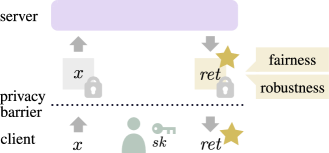
2(1.84,-1.52) Phoenix (Fig. 2)

Figure 1. A high-level overview of private and reliable inference in an FHE-based MLaaS setting using our system, Phoenix.

This Work: Prediction Guarantees with Client Data Privacy

.  We present Phoenix, which for the first time addresses the above question in a comprehensive manner, illustrated in Fig. 1. Phoenix enables FHE-execution of randomized smoothing (RS) (Cohen et al., 2019), a state-of-the-art method for obtaining reliability guarantees on top of neural network inference. Phoenix lifts the algorithmic building blocks of RS to FHE, utilizing recent advances in non-polynomial function approximation to solve the challenging task of executing the Argmax function in a private FHE-based setting. Making progress on this challenge in the context of RS is significant as (i) RS naturally enables guarantees such as fairness and robustness (Section 3.1), and (ii) the core building blocks are general and provide value outside of the RS context for establishing broader guarantees (Section 3.2).

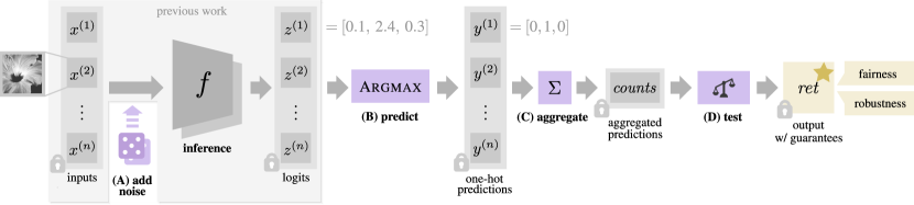
Figure 2. An illustration of Phoenix, which enables homomorphically encrypted neural network inference with guarantees. The symbol  denotes encryption of the value in an FHE scheme by the client.

Main Contributions

.  Our main contributions are:

• ArgmaxHE, an efficient and precise approximation of the challenging Argmax operator in RNS-CKKS FHE (Cheon et al., 2018b) (Section 5).

• Phoenix , which by utilizing ArgmaxHE and other novel building blocks, for the first time enables FHE-based MLaaS with useful robustness and fairness guarantees. (Section 6, Section 7).

• An extensive experimental evaluation of both instantiations of Phoenix, implemented in Microsoft SEAL (WA, 2020) (Section 8).

2. Motivation

We discuss the motivation for Phoenix, introducing examples that illustrate the need for reliability guarantees, and motivate the importance of obtaining such guarantees alongside client data privacy.

Example: Fair Loan Eligibility

.  Consider an ML system deployed by a financial institution in an MLaaS setting to automatically predict loan eligibility based on clients’ financial records. Recent work (Buolamwini and Gebru, 2018; Corbett-Davies et al., 2017; Kleinberg et al., 2017; Tatman and Kasten, 2017; Dwork et al., 2012) demonstrates that without any countermeasures, such a model may replicate biases in training data and make unfair decisions. For example, a loan application might be rejected based on a sensitive attribute of the client (e.g., race, age, or gender), or there could be pairs of individuals with only minor differences who unjustly receive different outcomes (see Section 4.4 for more details on these two interpretations of fairness—Phoenix focuses on the latter). Indeed, existing systems were shown to manifest unfair behavior in practice. For instance, the recidivism prediction algorithm COMPAS was found to unfairly treat black people (Julia Angwin and Kirchner, 2016). Ideally, the loan eligibility service would provide fairness guarantees, ensuring that every prediction for a client’s input is fair. In case no fair decision can be made automatically, the model refers the client to a human contact for manual assessment. Providing such a guarantee greatly improves the accountability of the system for both parties.

Example: Robust Medical Image Analysis

.  Consider the problem of medical image analysis, where patient data (MRI, X-ray or CT scans) is used for cancer diagnosis, retinopathy detection, lung disease classification, etc.  (Apostolidis and Papakostas, 2021). ML algorithms are increasingly used for such applications to reduce the worryingly high rate of medical error (Makary and Daniel, 2016). Such an algorithm, deployed as a cloud service, may be used by medical providers to assist in diagnosis, or even by patients as a form of second opinion. However, it was observed that such algorithms are particularly non-robust (Ma et al., 2021) to slight perturbations of input data, which could be due to a malicious actor, e.g., patients tampering with their reports to extract compensation (Paschali et al., 2018), or naturally-occurring measurement errors. As such perturbations may lead to needless costs or negative effects on patient’s health (Mangaokar et al., 2020), it is in the interest of both parties that the cloud service provides robustness guarantees. That is, the returned diagnosis is guaranteed to be robust to input data variations and can thus be deemed trustworthy. See Section 4.3 for a more formal discussion.

Reliability Guarantees Alongside Data Privacy

.  As the above examples illustrate, reliability guarantees can greatly benefit MLaaS deployments, prompting regulators to call for their use (Turpin et al., 2020; FDA, 2019; Comission, 2022), and researchers to actively investigate this area (Dwork et al., 2012; Yeom and Fredrikson, 2020; Ruoss et al., 2020; Gehr et al., 2018; Gowal et al., 2018; Cohen et al., 2019). However, ensuring reliable predictions does not address the important complementary concern of client data privacy, which becomes desirable and commonly required (Parliament and Council, 2016; Legislature, 2018) when dealing with sensitive user data, as is often the case in MLaaS setups. Latest privacy-preserving machine learning (Gilad-Bachrach et al., 2016; Chou et al., 2018; Brutzkus et al., 2019; Lou and Jiang, 2019; Liu et al., 2017; Juvekar et al., 2018; Mishra et al., 2020) methods such as FHE enable clients to utilize e.g., loan eligibility and medical diagnosis services without directly revealing their sensitive financial records (e.g., revenue) or medical imaging to the potentially untrusted service provider. While desirable, achieving both of these goals at the same time is difficult: methods that provide reliability guarantees often involve additional inference-time logic, which makes lifting computation to FHE in order to protect client data privacy significantly more challenging. Phoenix for the first time takes a major step in addressing this challenge, enabling the deployment of models which are both reliable and private.

3. Overview

We provide a high-level outline of Phoenix (Section 3.1), presenting all algorithmic building blocks needed to enable reliability guarantees via randomized smoothing. Further, we discuss alternative instantiations of Phoenix that enable different properties (Section 3.2), its threat model (Section 3.3), and why it needs to be deployed on the server (Section 3.4).

3.1. Overview of Phoenix

Phoenix (Fig. 2) leverages randomized smoothing to produce ML models with inference-time reliability guarantees. Key to enabling this in FHE is to combine existing techniques for evaluating neural networks in FHE (marked “previous work” in Fig. 2) with new FHE counterparts which handle additional inference-time operations (indicated by (A)–(D) in Fig. 2). In that way, Phoenix also enables FHE-execution of any future procedure which relies on one or more of these fundamental components (as we discuss shortly in Section 3.2).

Inference

.  The first ingredient is neural network inference: Consider a neural network $f$ classifying an input $x^{(i)}$ into one of $c$ classes. Concretely, $f$ outputs a vector of unnormalized scores $z^{(i)}$, called logits, and $f$ is said to classify $x^{(i)}$ to the class with the largest logit.

In the private MLaaS setting, the inputs $x^{(i)}$ are encrypted by the client using an FHE scheme (denoted by ). Ignoring the addition of noise (discussed shortly), the inputs are propagated through $f$ utilizing the homomorphic operations of the FHE scheme to obtain the logits $z^{(i)}$. In Fig. 2, this is illustrated for $c=3$ where $x^{(1)}$ is classified to the second class with logit value $z^{(1)}_{2}=2.4$. See Section 4.2 for a more detailed discussion of neural network inference in FHE.

Randomized Smoothing

.  A core paradigm employed by Phoenix is randomized smoothing (RS, detailed in Section 4.5). To obtain reliability guarantees, we add Gaussian random noise (A) to many copies of a single input $x^{(1)}=\dots=x^{(n)}$, and perform neural network inference on these noisy copies to get a set of logit vectors $z^{(i)}$.

Existing privacy-preserving machine learning systems would typically directly return the logits $z^{(i)}$ to the client for decryption (Gilad-Bachrach et al., 2016; Brutzkus et al., 2019; Dathathri et al., 2019; Lou and Jiang, 2021). However, to apply RS, Phoenix includes a predict step (B), which evaluates the Argmax function in FHE. In particular, this step transforms the logit vectors $z^{(i)}$ of unnormalized scores into one-hot vectors $y^{(i)}$ of size $c$, where a single non-zero entry $y^{(i)}_{j}$ encodes the index $j$ of the largest component $z_{j}^{(i)}$. For example, predicting the second class is represented by $[0,1,0]$.

Next, we aggregate the predictions (C) in a statistically sound way (details given in Section 6) to determine the index $k$ of the class most often predicted by the network, as well as the number of such predictions.

Finally, we perform a homomorphic version of a carefully calibrated statistical test (D), to obtain $\mathit{ret}$, the ciphertext returned to the client, containing the final prediction with reliability guarantees.

Obtaining Specific Guarantees

.  Depending on how it is employed, RS is able to produce different guarantees. In Section 6.1, we discuss local robustness (PhoenixR), i.e., guaranteeing that minor input perturbations such as slight changes of lighting conditions for images do not change the model prediction. Further, in Section 6.2 we adapt RS to support inference-time individual fairness guarantees (PhoenixF), ensuring that similar individuals are treated similarly.

3.2. Further Instantiations

The building blocks (A–D) of RS enabled by Phoenix are general. Thus, Phoenix can also be instantiated in configurations beyond those we consider. In particular, depending on the number of models used for inference, which subset of predictions is aggregated, and where noise is added, the output may satisfy different properties.

Namely, variants of RS have been proposed for various scenarios (Salman et al., 2019; Fischer et al., 2020; Yang et al., 2020; Chiang et al., 2020; Fischer et al., 2021; Kumar et al., 2021; Bojchevski et al., 2020; Peychev et al., 2022). For example, Peychev et al. (2022) combines RS with generative models to achieve provably fair representation learning, and Bojchevski et al. (2020) considers robust reasoning over graphs in the presence of perturbations on edge weights. To migrate these and similar techniques to FHE, the building blocks (A–D) can likely be reused with slight adaptions.

Further, Phoenix could be instantiated to enhance the privacy properties of PATE (Papernot et al., 2017), a state-of-the-art differentially private learning (Dwork et al., 2006) framework. In particular, executing PATE in an FHE-based private setup would preserve the confidentiality of the unlabeled dataset, making PATE more broadly applicable to scenarios where this data is private and sensitive. On a technical level, PATE uses an ensemble of models at the inference step, adding noise (A) to their aggregated predictions (B–C). This makes Phoenix particularly suitable for the task of lifting it to FHE.

Finally, as another example, addition of noise (A) and Argmax (B) are also fundamental components of the uncertainty quantification approach proposed by Wang et al. (2019).

We leave extending Phoenix to these settings to future work.

3.3. Threat Model and Security Notion

In this work, we consider a combination of two standard threat models: the two-party semi-honest attacker model from private NN inference (attackers (i)–(ii) below), and the standard active attacker model from robustness (attacker (iii) below). In particular, we consider three adversaries: (i) a semi-honest attacker on the server-side, which tries to learn the plaintext client input data $x$; (ii) a semi-honest attacker sitting on the network between client and server, also trying to learn $x$; and (iii) an active adversary on the client-side, which tries to imperceptibly corrupt client’s data $x$. As we will discuss in Section 4.3, adversary (iii) models both naturally occurring measurement errors and deliberate tampering.

The core security notion achieved by Phoenix is client data privacy (see Thm. 1 in Section 7.1). In particular, we do not aim to achieve the orthogonal notions of training set privacy or model privacy, which are concerned with maintaining the privacy of server’s data at training time or maintaining privacy of model data at inference time. Note that attacker (iii) is irrelevant for ensuring client data privacy. In addition, Phoenix satisfies reliability guarantees (see Thm. 2 in Section 7.2); only attacker (iii) is relevant for these properties.

3.4. Necessity of Computing on the Server

Phoenix executes RS fully on the server. Due to the active client-side adversary ((iii) in Section 3.3), offloading RS to clients would make it impossible for the service provider to guarantee reliability, as such guarantees rely on careful parameter choices and sound execution of the certification procedure. For example, in the case of fairness, setting unsuitable parameters of RS on the client side (maliciously or by accident, both of which are captured by the active client-side adversary) would allow the clients to use the service to obtain unfair predictions, nullifying the efforts of the service provider to prove fairness compliance to external auditors. See Section 7.2 for a thorough correctness analysis of guarantees produced by Phoenix.

An additional privacy benefit of server-side computation, orthogonal to client data privacy, is in reducing the threat of model stealing attacks (Tramèr et al., 2016; Reith et al., 2019), where clients aim to recover the details of the proprietary model $f$ given the logit vector $z$ of unnormalized scores. Most prior work on neural network inference in FHE is vulnerable to such attacks as it returns the encryption of $z$ to the client (Gilad-Bachrach et al., 2016; Brutzkus et al., 2019; Dathathri et al., 2019; Lou and Jiang, 2021), who then needs to apply Argmax on the decrypted vector to obtain the prediction. Merely approximating the score normalization, i.e., executing the softmax function in FHE (Lee et al., 2021a), was shown to not offer meaningful protection (Truong et al., 2021). In contrast, applying the approximation of Argmax to $z$ in FHE on the server (as done in Phoenix) allows the server to return a one-hot prediction vector to the client. As illustrated by the model access hierarchy of Jagielski et al. (2020), this greatly reduces the risk of model stealing.

Finally, client-side RS would increase the communication cost, as well as the effort for transitioning existing systems to inference with guarantees or later modifying the parameters or offered guarantees.

4. Background

We next introduce the background necessary to present Phoenix. In Section 4.1 and Section 4.2 we recap fully homomorphic encryption and how it is commonly used for privacy-preserving neural network inference. In Section 4.3 and Section 4.4 we formally introduce the two types of reliability guarantees considered in Phoenix: local robustness and individual fairness. Finally, in Section 4.5 we discuss randomized smoothing, a technique commonly used to provide such guarantees. Phoenix lifts this technique to fully homomorphic encryption to ensure predictions enjoy both client data privacy as well as reliability guarantees.

4.1. Leveled Fully Homomorphic Encryption with RNS-CKKS

An asymmetric encryption scheme with public key $pk$ and secret key $sk$ is homomorphic w.r.t. some operation $\ast$ if there exists an operation $\stackMath\mathbin{\stackinset{c}{0ex}{c}{0ex}{\ast}{\bigcirc}}$, efficiently computable without knowing $sk$, s.t. for each pair of messages $x,y\in\mathcal{M}$, where $\mathcal{M}$ is a field, it holds that

$$\text{{Dec}}_{sk}({\text{{Enc}}_{pk}({x})\stackMath\mathbin{\stackinset{c}{0ex}{c}{0ex}{\ast}{\bigcirc}}\text{{Enc}}_{pk}({y})})=x\ast y.$$

Here, for a ciphertext space $\mathcal{C}$, the functions $\texttt{Enc}_{pk}\colon\mathcal{M}\to\mathcal{C}$ and $\texttt{Dec}_{sk}\colon\mathcal{C}\to\mathcal{M}$ denote the (often randomized) encryption using $pk$, and decryption using $sk$, respectively. Fully homomorphic encryption (FHE) schemes (Gentry, 2009; Brakerski et al., 2012; Fan and Vercauteren, 2012; Cheon et al., 2017; Ducas and Micciancio, 2015; Chillotti et al., 2016, 2021; Cheon et al., 2018b) are those homomorphic w.r.t. all field operations in $\mathcal{M}$. As such, FHE can be used to evaluate arbitrary arithmetic circuits (i.e., computations of fixed size and structure) on underlying plaintexts. Note that as such circuits do not allow for control flow (e.g., branching or loops), reflecting arbitrary computation in FHE can be challenging and/or very expensive.

RNS-CKKS

.  In this work, we focus on RNS-CKKS (Cheon et al., 2018b)—an efficient implementation of the CKKS (Cheon et al., 2017) FHE scheme. The plaintexts and ciphertexts of RNS-CKKS consist of elements of the polynomial ring of degree $N$ with integer coefficients modulo $Q=\prod_{l=0}^{L}Q_{l}$, where $Q_{l}$ are distinct primes, and $N$ and $L$ are parameters. A message is the atomic unit of information that can be represented in the scheme. We consider the message space $\mathcal{M}=\mathbb{R}^{M}$ (technically, $\mathbb{R}$ is represented as fixed-point numbers), where $M=\frac{N}{2}$ denotes the number of so-called slots in a message. To encrypt, all slots in a message $x\in\mathcal{M}$ are multiplied by the initial scale $\Delta\in\mathbb{R}$, and the result is encoded to get a plaintext $\texttt{Ecd}(x)\in\mathcal{P}$, and then encrypted using a public key $pk$ to obtain a ciphertext $\text{{Enc}}_{pk}({x})\in\mathcal{C}$.

Below, we list the homomorphic evaluation primitives of RNS-CKKS. Here, all binary operations ${\stackMath\mathbin{\stackinset{c}{0ex}{c}{0ex}{\ast}{\bigcirc}}\colon\mathcal{C}\times\mathcal{C}\to\mathcal{C}}$ have a variant ${\stackMath\mathbin{\stackinset{c}{0ex}{c}{0ex}{\ast}{\bigcirc}}_{p}\colon\mathcal{C}\times\mathcal{M}\to\mathcal{C}}$, where one argument is a plaintext.

• Addition/subtraction: $\oplus$ and $\ominus$ perform slot-wise (vectorized) addition of the messages underlying the operands.

• Multiplication: $\otimes$ performs slot-wise multiplication.

• Rotation: RotL: $\mathcal{C}\times\mathbb{N}\to\mathcal{C}$ and RotR: $\mathcal{C}\times\mathbb{N}\to\mathcal{C}$ cyclically rotate the slots of the underlying message by the given number of steps left and right, respectively.

For example, for $M=3$ and $\mathcal{M}=\mathbb{R}^{3}$, it is

$$\texttt{RotR}(\text{{Enc}}_{pk}({[a,b,c]}),1)\otimes_{p}[2,3,1]\ =\ \text{{Enc}}_{pk}({[2c,3a,b]}).$$

RNS-CKKS is a leveled FHE scheme: only computation up to multiplicative depth $L$ is supported. That is, any computation path can include at most $L$ multiplications $\otimes$ or $\otimes_{p}$ (but arbitrarily many other operations). Bootstrapping (Gentry, 2009; Cheon et al., 2018a) is designed to overcome this limitation, however, it is still largely impractical (Lee et al., 2021a, b), so the RNS-CKKS scheme is most often used in leveled mode.

Typical choices of $N$ are $N\geq 2^{15}$, enabling powerful single-instruction-multiple-data (SIMD) batching of computation. This, with the support for fixed-point computation on real numbers, makes RNS-CKKS the arguably most popular choice for private ML applications (Dathathri et al., 2019, 2020; Ishiyama et al., 2020; Lee et al., 2021a, b; Lou and Jiang, 2021). Unfortunately, choosing a large $L$ incurs a significant performance penalty. Therefore, representing the computation in a way that minimizes multiplicative depth is a key challenge for practical deployments of RNS-CKKS. Phoenix tackles this challenge when designing an efficient approximation of Argmax for FHE, which we will present in Section 5.

4.2. Privacy-Preserving Neural Network Inference

We next describe how FHE is used to perform privacy-preserving inference on neural network models.

Setting

.  We focus on the classification task, where for given inputs $x\in\mathbb{R}^{d}$ from $c$ classes, a classifier $f\colon\mathbb{R}^{d}\to\mathbb{R}^{c}$ maps inputs to class scores (discussed shortly). We model $f$ as a neural network with $k$ successively applied layers. As a first step, in this work we focus on fully-connected ReLU networks: each layer $f_{i}\colon\mathbb{R}^{n_{i-1}}\to\mathbb{R}^{n_{i}}$ of the network either represents a linear transformation $f_{i}(t)=W_{i}t+b_{i}$ of the input $t\in\mathbb{R}^{n_{i-1}}$, where $W_{i}\in\mathbb{R}^{n_{i}\times n_{i-1}}$ and $b_{i}\in\mathbb{R}^{n_{i}}$, or a non-linear ReLU activation function $f_{i}(t)=max(0,t)$, where $max$ is applied componentwise. Layers $f_{1}$ and $f_{k}$ are generally linear, with $n_{0}=d$, and $n_{k}=c$. The output of the full network $z=f(x)=f_{k}\circ\ldots\circ f_{1}(x)\in\mathbb{R}^{c}$ is a vector of unnormalized scores, called logits, for each class (see also Fig. 2). To simplify the discussion, we assume that the elements of $z$ are unique. We say that for an input $x$ the class with the highest logit is the class predicted by $f(x)$. For $[c]:=\{1,\ldots,c\}$, we define $F\colon\mathbb{R}^{d}\to[c]$ to compute the class $F(x)$ predicted by $f(x)$.

Inference & Batching

.  We now discuss how neural network inference (that is, the evaluation of $f(x)$) is commonly encoded in RNS-CKKS (Dathathri et al., 2019, 2020; Lou and Jiang, 2021). For an input $x\in\mathbb{R}^{d}$, we write $[x_{1},\ldots,x_{d},0^{M-d}]$ to denote either an RNS-CKKS message underlying the plaintext $\texttt{Ecd}(x)\in\mathcal{P}$, or the corresponding ciphertext $\text{{Enc}}_{pk}({x})\in\mathcal{C}$, where the distinction is clear from the context. Here, $0^{M-d}$ denotes $M-d$ zeroes padding the message to $M$ slots.

To efficiently evaluate a fully-connected layer $f_{i}({s})=W_{i}s+b_{i}$ on ciphertext $s$ and plaintexts $W_{i}$ and $b_{i}$, we use the hybrid matrix-vector product (MVP) algorithm of Juvekar et al. (2018). This algorithm uses a sequence of $\oplus_{p}$, $\otimes_{p}$, and RotL operations to compute an MVP. It requires RotL to produce valid cyclic rotations of $s_{1},\ldots,s_{d}$ in the first $d$ (not $M$) slots of the ciphertext. To satisfy this, the MVP algorithm is applied on a duplicated version $s^{\prime}$ of the input message $s$, namely $s^{\prime}=[s_{1},\ldots,s_{d},s_{1},\ldots,s_{d},0^{M-2d}]$, obtained by $s^{\prime}\leftarrow s\oplus\texttt{RotR}([s_{1},\ldots,s_{d},0^{M-d}],d)$.

Recall that all operations to be performed in FHE need to be reduced to the primitives of the RNS-CKKS scheme. As a result, evaluating non-polynomial functions such as ReLU is practically infeasible. Like previous work Dathathri et al. (2019), we replace ReLU with the learnable square activation function $c_{2}x^{2}+c_{1}x$, where coefficients $c_{2}$ and $c_{1}$ are optimized during training.

It is common to use $M\gg 2d$ and leverage SIMD batching to simultaneously perform inference on a batch of $B=M/2d$ (assuming $2d$ divides $M$) duplicated inputs. Using rotations and $\oplus$ we put $B$ duplicated inputs in one ciphertext, obtaining

(1) $$\bar{x}=[x^{(1)}_{1},\ldots,x^{(1)}_{2d},~{}\cdots~{},x^{(B)}_{1},\ldots,x^{(B)}_{2d}],$$

which consists of $B$ blocks of size $2d$ each. Propagating this through the network, we obtain a batch of logits

$$\bar{z}=[z^{(1)}_{1},\ldots,z^{(1)}_{c},\#^{2d-c},~{}\cdots~{},z^{(B)}_{1},\ldots,z^{(B)}_{c},\#^{2d-c}],$$

where we use $\#$ to denote irrelevant slots which contain arbitrary values, produced as a by-product of inference.

In Section 6, we will describe how Phoenix relies on all introduced techniques for private inference in reliable neural networks.

4.3. Local Robustness

The discovery of adversarial examples (Szegedy et al., 2013; Biggio et al., 2013), seemingly benign inputs that cause mispredictions of neural networks, lead to the investigation of robustness of neural networks. This is commonly formalized as local robustness: a model $F$ is locally-robust in the $\ell_{p}$ ball of radius $R$ around input $x$ if, for some class $k$,

(2) $$\forall\delta,\|\delta\|_{p}<R\colon\quad{F(x+\delta)}=k.$$

In an attempt to mitigate adversarial examples, various heuristic methods (Goodfellow et al., 2015; Kurakin et al., 2017) produce empirically robust networks. However, such models have been repeatedly successfully attacked (Athalye et al., 2018; Carlini et al., 2019; Tramèr et al., 2020) and are hence not suited to safety-critical scenarios. In contrast, robustness certification methods (Gehr et al., 2018; Gowal et al., 2018; Cohen et al., 2019; Singh et al., 2019; Xu et al., 2020) provide rigorous mathematical guarantees that $F$ is locally-robust around some input $x$ according to Eq. 2, for some choice of $p$ and $R$.

In Phoenix, we consider $\ell_{2}$ as well as $\ell_{1}$ local robustness certification (i.e., ${p=2}$ and ${p=1}$ in Eq. 2). However, Phoenix can likely be extended to other settings, as we will discuss in Section 4.5.

Attack Vectors & Natural Changes

.  As discussed above, local robustness offers protection against data perturbations. In practice, there are two different sources of such perturbations. First, an adversary may deliberately and imperceptibly perturb client data before or after it is acquired by the client, e.g., compromising client’s data collection, storage, or loading procedure (Bagdasaryan and Shmatikov, 2021). Second, even in the absence of deliberate perturbations, ML models are susceptible to volatile behavior under natural changes such as measurement noise or lighting conditions—in fact, this is a key motivation for robustness (Engstrom et al., 2019; Hendrycks and Dietterich, 2019; Wong and Kolter, 2021; Laidlaw et al., 2021; Hendrycks et al., 2021; Taori et al., 2020). The active client-side attacker introduced in Section 3.3 models both these sources of perturbations.

4.4. Individual Fairness

The notion of fairness of ML models has no universal definition in the literature (Caton and Haas, 2020), however group fairness (Dwork et al., 2012; Hardt et al., 2016) and individual fairness (Dwork et al., 2012) are the most prevalent notions in the research community. Phoenix focuses on individual fairness, whose guarantees could be perceived as stronger, as models that obey group fairness for certain groups can still discriminate against other population subgroups or individual users (Kearns et al., 2018).

Individual fairness states a model should treat similar individuals similarly, most often formalized as metric fairness (Dwork et al., 2012; Ruoss et al., 2020; Yurochkin et al., 2020; Mukherjee et al., 2020):

(3) $$\forall x_{1},x_{2}\in\mathcal{X}\colon\quad d_{y}(F(x_{1}),F(x_{2}))\leq Ld_{x}(x_{1},x_{2}),$$

where $L\in\mathbb{R}^{>0}$, and $F\colon\mathcal{X}\to\mathcal{Y}$ maps the input space $\mathcal{X}$ with metric $d_{x}$ to the output space $\mathcal{Y}$ with metric $d_{y}$. Intuitively, for individuals $x_{1}$ and $x_{2}$ close w.r.t. $d_{x}$, the difference in the output of $F$ must not exceed a certain upper bound, proportional to the input distance.

4.5. Randomized Smoothing

We now recap randomized smoothing, which we will use in Section 6 to provide fairness and robustness guarantees.

Smoothed Classifier

.  Randomized smoothing (RS) (Cohen et al., 2019) is a procedure that at inference time transforms a base classifier $F\colon\mathbb{R}^{d}\to[c]$ (e.g., a trained neural network) into a smoothed classifier $G\colon\mathbb{R}^{d}\to[c]$ as follows. For given input $x$, the classifier $G$ returns the most probable prediction of $F$ under isotropic Gaussian perturbations of $x$. Formally, for $\varepsilon\sim\mathcal{N}(0,\sigma^{2}I_{d})$, where $I_{d}$ is the $d$-dimensional identity matrix and $\sigma\in\mathbb{R}^{\geq 0}$ is the standard deviation, we define

(4) $$G(x):=\operatorname*{arg\,max}_{j\in[c]}p_{j}\quad\text{with}\quad p_{j}:=\mathbb{P}(F(x+\varepsilon)=j).$$

The smoothed classifier $G$ behaves similarly to $F$, but with the additional property that slight changes in the input only result in slight changes of the output. In particular, $G$ is guaranteed to be locally-robust (see Eq. 2) in the $\ell_{2}$ ball of radius $R$ around input $x$, where $R$ can be determined as a function of $x$, $F$ and $\sigma$. In Section 6, we will show how RS can also be used to enforce individual fairness.

Algorithm 1 Certification with Randomized Smoothing (Fischer et al., 2021)

1:# a subroutine to evaluate $f$ at $x$ under Gaussian noise

2:function SampleUnderNoise($f$, $x$, $n$, $\sigma$)

3: $\mathit{counts}$ $\leftarrow$ $[{0,\ldots,0}]$ of size $c$

4: for $i\leftarrow 1$ to $n$ do

5:  $\varepsilon\leftarrow$ sample from $\mathcal{N}(0,\sigma^{2}I_{d})$

6:  $x^{\prime}\leftarrow x+\varepsilon$

7:  $z\leftarrow f(x^{\prime})$

8:  $y\leftarrow$ Argmax($z$) $\triangleright$ one-hot vector

9:  $\mathit{counts}\leftarrow\mathit{counts}+y$

10: return $\mathit{counts}$

11:# evaluate and certify the robustness of $g$ at $x$

12:function Certify($f$, $x$, $\sigma$, $n$, $n_{0}$, $\tau$, $\alpha$)

13: $\mathit{counts}_{0}$ $\leftarrow$ SampleUnderNoise($f$, $x$, $n_{0}$, $\sigma$)

14: $k\leftarrow$ ArgmaxIdx($\mathit{counts}_{0}$) $\triangleright$ integer index

15: $\mathit{counts}$ $\leftarrow$ SampleUnderNoise($f$, $x$, $n$, $\sigma$)

16: $pv\leftarrow$BinPValue($counts[k]$, $n$, $\tau$)

17: if $pv\leq\alpha$ return $k$ else abstain

Probabilistic Certification

.  Unfortunately, exactly computing $p_{j}$ in Eq. 4, required to determine both $G(x)$ and $R$, is typically intractable (for most $F$). However, using Monte Carlo sampling, $p_{j}$ can be lower-bounded by $\underline{p_{j}}$ with confidence $1-\alpha$. From this, for fixed target radius $R\in\mathbb{R}^{\geq 0}$, we can say that $G(x)=j$ if $\underline{p_{j}}>\tau=\Phi(R/\sigma)$ with the same confidence $1-\alpha$, where $\Phi$ denotes the standard Gaussian CDF. SampleUnderNoise in Alg. 1 follows this approach to sample $n$ Gaussian perturbations of input $x$ with standard deviation $\sigma$, and count the number of predictions of $F$ for each class.

For a target $R$ and error upper bound $\alpha$, we can check whether this sampling-based approximation satisfies Eq. 2 with probability at least $1-\alpha$ using a statistical test. In Alg. 1, we show the function Certify performing this step, inspired by Fischer et al. (2021).

To ensure statistical soundness, the function first uses $n_{0}$ samples of $F(x+\varepsilon)$ to guess the most likely class $k$ predicted by $G$. Note that this preliminary counting procedure can use any heuristic to guess $k$, as this does not affect the algorithm soundness. We exploit this in Section 6.1, where we introduce the soft preliminary counting heuristic.

Given $k$, Certify further performs a one-sided binomial test (16) on a fresh set of $n$ samples, to show (up to error probability $\alpha$) that the probability $p_{k}$ for $G$ to predict $k$ is at least $\tau$, and thus the certified radius is at least $R$. If the test fails, the function returns an “abstain” decision. Otherwise, the function returns the final prediction $k$, guaranteed to satisfy Eq. 2 with probability at least $1-\alpha$. See (Cohen et al., 2019, Theorem 1 and Proposition 2) for a proof.

Note that in Fig. 2, we do not make a distinction between preliminary (13) and main counting (15). While these are conceptually independent procedures, Phoenix heavily relies on batching (Section 4.2) to efficiently execute them jointly (discussed in Section 6).

RS relies on several algorithmic building blocks such as Argmax and statistical testing, which are challenging to perform in FHE. Phoenix overcomes this (Sections 5–6) and is instantiated to obtain local robustness and individual fairness guarantees via RS.

Generalizations

.  RS has been extended beyond $\ell_{2}$ certification in the setting of classification to a wide range of perturbation types (Salman et al., 2019; Fischer et al., 2020; Yang et al., 2020) and settings (Chiang et al., 2020; Fischer et al., 2021; Kumar et al., 2021). For example, Yang et al. (2020) show that sampling uniform noise $\varepsilon\sim\mathcal{U}(-\eta,\eta)$ in place of Gaussian noise (5 of Alg. 1) and executing the rest of RS as usual leads to an $\ell_{1}$ robustness certificate with radius $R=2\eta(\tau-0.5)$. Further, any $R$ certified in the $\ell_{2}$ case directly implies $\ell_{\infty}$ robustness with radius $R/\sqrt{d}$, where $d$ is the input dimension. In our experimental evaluation in Section 8 we explore both $\ell_{2}$ and $\ell_{1}$ certification.

5. Approximating the Argmax operator in FHE

Recall the key algorithmic building blocks of Phoenix visualized in Fig. 2. While some steps can easily be performed in FHE, a key challenge is posed by the Argmax step (B): as FHE does not allow evaluation of control flow (e.g., branching), and ciphertext comparison (e.g., checking inequality) is not directly supported by the homomorphic primitives of the RNS-CKKS FHE scheme, we cannot implement Argmax in the canonical way. Instead, we aim for an approximation. Formally, our goal is to approximate the following function on an RNS-CKKS ciphertext logit vector:

(5) $$[z_{1},\ldots,z_{c},0^{M-c}]\to[y_{1},\ldots,y_{c},\#^{M-c}],$$

where $y_{i}=1$ for the index $i$ corresponding to the largest value among $z_{i}$ (and $0$ elsewhere). Recall that we assume $z_{i}$ are unique.

In the following, we present the first efficient approximation of Argmax for RNS-CKKS (we discuss related work in Section 9). Our key insight is that Argmax can be expressed via simple arithmetic operations and the sign function, for which efficient RNS-CKKS approximations exist. For careful parameter choices and appropriate conditions (introduced shortly), we achieve both efficiency and the ability to bound the error of our approximation, guaranteeing the soundness of reliability guarantees returned by Phoenix.

Sign Function Approximation

.  To efficiently realize Argmax, we rely on a polynomial approximation of the sign function. In particular, we utilize recent work (Cheon et al., 2020) that efficiently approximates

$$\text{{Sgn}}(x)\vcentcolon=\begin{cases}\phantom{-}1&\text{if~{}}x>0\\ \phantom{-}0&\text{if~{}}x=0\\ -1&\text{if~{}}x<0\end{cases}$$

in RNS-CKKS for $x\in[-1,1]$. The proposed approximation SgnHE composes odd polynomials $p_{n}$ and $q_{n}$ parametrized by integer $n$:

(6) $$\text{{Sgn}}(x)\sim\text{{SgnHE($d_{q},d_{p},n,x$)}}=p_{n}^{d_{p}}\circ q_{n}^{d_{q}}$$

For desired precision parameters $\phi$ and $\psi$, we can choose integers $d_{q}(\phi)$ and $d_{p}(\psi)$ such that the approximation is $(\phi,\psi)$-close, meaning that for $x\in[\phi,1]$ (resp. $x\in[-1,-\phi]$), the output of SgnHE is guaranteed to be in $[1-2^{-\psi},1]$ (resp. $[-1,-1+2^{-\psi}]$). Note that for inputs $x\in[-1,-\phi]\cup[\phi,1]$, SngHE never outputs $0$.

As suggested in (Cheon et al., 2020), we choose $n=4$ to efficiently evaluate the polynomials using the Baby-Step Giant-Step algorithm (Han and Ki, 2020). This results in a multiplicative depth of SgnHE of $4(d_{p}+d_{q})$. We remark that future iterations of Phoenix could benefit from ongoing work on optimizing non-polynomial function approximation in FHE, such as the latest extension of Lee et al. (2022).

Algorithm 2 Approximation of Argmax for RNS-CKKS

1:function ArgmaxHE

2: Inputs: $z=[z_{1},\ldots,z_{c},0^{M-c}]$, $d_{q}^{(1)}$, $d_{p}^{(1)}$, $d_{q}^{(2)}$, $d_{p}^{(2)}$

3: Output: $y=[y_{1},\ldots,y_{c},\#^{M-c}]$ as in Eq. 5

4: $z\leftarrow z\oplus\texttt{RotR}(z,c)$

5: $\mathit{scores}\leftarrow[0^{M}]$

6: $z_{rot}\leftarrow z$

7: for $\mathit{offset}\leftarrow 1$ to $c-1$ do

8:  $z_{rot}\leftarrow\texttt{RotL}(z_{rot},1)$

9:  $\mathit{diff}\leftarrow z\ominus z_{rot}$

10:  $\mathit{signs}\leftarrow\text{{SgnHE($d_{q}^{(1)}$, $d_{p}^{(1)}$, 4, $\mathit{diff}$)}}$

11:  $\mathit{scores}\leftarrow\mathit{scores}\oplus\mathit{signs}$

12: $\mathit{scores}\leftarrow(\mathit{scores}\otimes_{p}[\frac{1}{2c-2}^{M}])\ominus_{p}[\frac{c-2}{2c-2}^{M}]$

13: $\mathit{scores}\leftarrow\mathit{scores}\otimes_{p}[1^{c},0^{M-c}]$

14: $y\leftarrow\text{{SgnHE($d_{q}^{(2)}$, $d_{p}^{(2)}$, 4, $\mathit{scores}$)}}$

15: $y\leftarrow(y\otimes_{p}[\frac{1}{2}^{M}])\oplus_{p}[\frac{1}{2}^{M}]$

16: return $y$

Argmax Approximation

.  In Alg. 2 we present ArgmaxHE, which efficiently approximates Argmax via SgnHE. Our construction is similar to the ideas of (Sébert et al., 2021; Iliashenko and Zucca, 2021) (discussed in Section 9), but specifically targets the RNS-CKKS scheme. The procedure takes as input a logit ciphertext $z$ and produces an output ciphertext $y$, generalizing naturally to batched computation. ArgmaxHE relies on SgnHE and is parameterized by $d_{q}^{(1)}$, $d_{p}^{(1)}$, $d_{q}^{(2)}$, $d_{p}^{(2)}$ used for SgnHE.

In Fig. 3, we illustrate how Alg. 2 processes a toy example. The algorithm first duplicates the logits (4) and initializes $\mathit{scores}$ to $0$. Then, for each offset $\mathit{offset}\in[1,c-1]$ we construct $\mathit{diff}$ (9), such that $\mathit{diff}_{i}=z_{i}-z_{j}$, where $j=(i+\mathit{offset}-1)\ \%\ (c+1)$ takes the values $i+1,i+2,\ldots,i-1$ in successive iterations. For example, in Fig. 3, the first iteration with $\mathit{offset}=1$ computes in $\mathit{diff}$ the slot-wise difference between $z$ and $z_{rot}$ to obtain $\mathit{diff}_{0}=0.3-0.4=-0.1$. Applying SgnHE (10) to these differences maps them to $\{-1,1\}$ (see $\mathit{signs}$ in Fig. 3). Summing these up yields $\mathit{scores}_{i}=\sum_{j\neq i}\left(2\cdot\mathbbm{1}_{z_{i}>z_{j}}-1\right)$ for each logit, where $\mathbbm{1}_{\phi}=1$ if $\phi$ holds, and $0$ otherwise. We next argue that assuming $c$ is even and $z_{i}$ are unique, the first $c$ slots of $\mathit{scores}$ are exactly a permutation of $S:=[-(c-1),-(c-3),\ldots,-1,1,\ldots,c-3,c-1]$. Assume w.l.o.g. that the logits are sorted increasingly as $z_{1}<z_{2}<\cdots<z_{c}$. Then, for $i\in\{1,\ldots,c\}$, it is $\mathit{scores}_{i}=\sum_{j<i}1+\sum_{j>i}(-1)=(2i-c-1)$, giving the array $S$ above. As the logits are not necessarily sorted, the resulting scores for $i\in\{1,\ldots,c\}$ are a permutation of $S$. By construction, the index $k$ at which we find $c-1$ is the index of the largest logit $z_{k}$. For example, in Fig. 3, the value of $\mathit{scores}$ computed in the last iteration ($\mathit{offset}=3$) contains the value $3$ at index $k=1$.

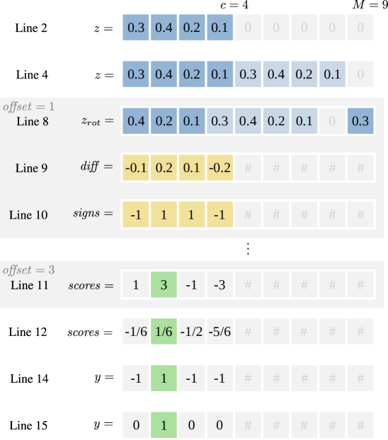
Figure 3. Example run of Alg. 2.

In order to identify $k$, we transform the first $c$ slots of $\mathit{scores}$ to $[-1,\ldots,-1/(2c-2),1/(2c-2)]$ (12), multiply $\mathit{scores}$ with $[1^{c},0^{M-c}]$ to clear the unused values which stabilizes the ciphertext (13), and use another SgnHE (14) to map all of the first $c$ slots but slot $k$ to $-1$. The final transformation (15) produces the desired one-hot vector.

Input Requirement and Error Bound

.  As we previously noted, SgnHE provably approximates Sgn well if, for small $\phi$, its input is in $[-1,-\phi]\cup[\phi,1]$. In particular, the two invocations of SgnHE in 10 and 14 require the inputs $\mathit{diff}$ and $\mathit{scores}$, respectively, to satisfy this requirement in order to bound the error of Alg. 2.

In Section 7.2, we will introduce two conditions on the logit vectors $z\in\mathbb{R}^{c}$ returned by the neural network $f$ in Phoenix, which (assuming appropriate parameter choices, also discussed in Section 7.2) ensure that the above input requirement provably holds. By analyzing the probability of these conditions to be violated, we will derive an upper bound on the overall error probability of Phoenix, i.e., the probability that a returned guarantee does not hold. We will further discuss the values of this bound in practice, concluding that the introduced conditions are not restrictive.

Multiplicative Depth

.  By modifying the polynomials involved in the evaluation of SgnHE, we can absorb the applications of the $\otimes_{p}$ operation in 12 and 15, reducing the multiplicative depth. As a result, the ArgmaxHE function in Alg. 2 has a multiplicative depth of $\lambda_{\mathit{argmax}}=4\cdot(d_{q}^{(1)}+d_{p}^{(1)}+d_{q}^{(2)}+d_{p}^{(2)})+1$, where $1$ arises from 13.

6. Private Randomized Smoothing

Next, we present how to evaluate RS (see Section 4.5) in the RNS-CKKS FHE scheme, leveraging ArgmaxHE from Section 5. In particular, we discuss how to homomorphically execute Alg. 1 and obtain local robustness guarantees (PhoenixR, Section 6.1), and how to extend this approach to guarantee individual fairness (PhoenixF, Section 6.2).

6.1. Robustness Guarantees

PhoenixR instantiates Phoenix for robustness certification by evaluating Certify on the server, lifted to FHE. In the following, we present the main challenges in achieving this and how Phoenix overcomes them. First, we discuss how we implement the SampleUnderNoise subroutine, including the considerations needed to efficiently execute neural network inference. Then, we introduce the idea of using soft preliminary counting to improve efficiency, before we describe how to implement the statistical test of Certify.

Sampling under Noise

.  The client provides a single encrypted input $x=[x_{0},\ldots,x_{d},0^{M-d}]$ to PhoenixR. As we require $n$ copies of $x$ in 6, we use a sequence of RotR and $\oplus$ operations to create $n$ duplicated copies $\{x^{(1)},\ldots,x^{(n)}\}$ of $x$, packed in $n/B$ ciphertexts as in Eq. 1, where $B=M/(2d)$ is the batch size. Note that all RS parameters, including $n$, are set by the server, as noted in Section 3.4.

Next, we independently sample $n$ Gaussian noise vectors according to 5, and use $\oplus_{p}$ to homomorphically add the noise to batched duplicated inputs. We next apply batched neural network inference, described shortly, to obtain batched logit vectors $z^{(i)}$, further reduced to a single ciphertext $\bar{z}$.

Inference

.  Recall that in the pipeline of Fig. 2, the inputs $x^{(i)}$ are encrypted using FHE scheme. To homomorphically evaluate the neural network $f$ in the inference step (7 of Alg. 1), we rely on methods from related work discussed in Section 4.2. Namely, we directly adopt the described approaches to evaluate $n_{\mathit{lin}}$ linear and $n_{\mathit{act}}$ ReLU layers with multiplicative depth of $\lambda_{\mathit{inf}}=2(n_{\mathit{lin}}+n_{\mathit{act}})-1$, and heavily utilize SIMD batching, adapting it to our use-case to reduce the number of expensive FHE operations.

In particular, as commonly $2d\ll M$, we can batch the inputs $x^{(i)}$ in $M/(2d)$ ciphertexts. Note that this is in contrast to most MLaaS setups, where inference is typically only performed on a single input at a time and SIMD batching therefore cannot be effectively utilized (Dathathri et al., 2019; Lou and Jiang, 2019). Next, as inference transforms each $2d$-dimensional input into a $c$-dimensional logit vector, and commonly $c\ll 2d$, we can further batch the logit vectors $z^{(i)}$, again using rotations, $\oplus$, and masking of $\#$ values using $\otimes_{p}$ (which adds $\lambda_{\mathit{batching}}=1$ to the multiplicative depth). This reduces the number of ciphertext inputs to the costly prediction step (discussed shortly), where it is typically possible to place all logit vectors into a single ciphertext $\bar{z}$.

Prediction and Aggregation

.  For the prediction step (8), we apply ArgmaxHE (Section 5) to $\bar{z}$ to obtain $\bar{y}$, a ciphertext of batched one-hot prediction vectors. To aggregate them (9), we use a simple variation of the RotateAndSum algorithm (Juvekar et al., 2018), which repeatedly applies rotations and $\oplus$. SampleUnderNoise returns the ciphertext

$$\mathit{counts}=[\mathit{cnt}_{1},\ldots,\mathit{cnt}_{c},\#^{M-c}]$$

containing the number of times each class was predicted.

Soft Preliminary Counting

.  Determining the most likely class $k$ based on $\mathit{counts}_{0}$ requires two invocations of ArgmaxHE (8 and 14), significantly increasing the depth of Certify.

Recall from Section 4.5 that using a heuristic during preliminary counting does not affect the soundness of RS. Following this, we introduce the soft preliminary counting heuristic. Namely, when computing $\mathit{counts}_{0}$, instead of invoking ArgmaxHE to compute one-hot predictions $y$, we simply rescale $z$ by $1/n$ (by accordingly scaling the weights of $f$) to obtain a rough approximation of $y$. Consequently, the result returned in 10 holds the average of all logit vectors.

Avoiding another invocation of ArgmaxHE greatly reduces the multiplicative depth of PhoenixR, which would otherwise be prohibitive. At the same time, soft counting does not affect the soundness of the guarantees, and as we demonstrate in Section 8, it rarely impacts the decisions of Certify. See App. B for further discussion.

Statistical Testing

.  We next describe how to evaluate the statistical test in 16–17, which provides a robustness guarantee.

Let $p_{k}$ denote the probability that the smoothed model $G$ (Eq. 4) predicts $k$ as computed in 14. The one-sided binomial test attempts to prove that $p_{k}>\tau$ with error probability at most $\alpha$. To this end, it computes the $p$-value $pv=1-\textsc{BinCDF}(\mathit{counts}[k]-1;n,\tau)$, the probability of predicting the class $k$ at least $\mathit{counts}[k]$ out of $n$ times under the worst case $p_{k}=\tau$ of the null hypothesis $p_{k}\leq\tau$, where BinCDF denotes the binomial CDF.

Computing BinCDF on $\mathit{counts}[k]$ involves approximating the incomplete beta function, which is not easily reducible to FHE primitives. To overcome this, we rephrase the test using the following observation: For fixed $n$ and $\tau$, the p-value $pv$ is strictly decreasing w.r.t. $\mathit{counts}[k]$. Thus, we employ binary search to find $\mathit{target}$, the smallest value of $\mathit{counts}[k]$ for which $pv\leq\alpha$, i.e., the test passes. We visualize this in Fig. 4, where $k=3$, and $\mathit{target}=6$.

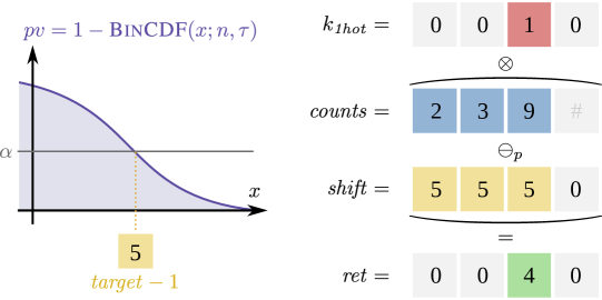
Figure 4. The statistical test of Phoenix, illustrated on an example.

Let $k_{\mathit{1hot}}$ denote the one-hot vector encoding the predicted class, obtained by multiplying the result of ArgmaxHE in 14 with $[1^{c},0^{M-c}]$ using $\otimes_{p}$, such that the non-zero slot is at index $k$. The server returns a ciphertext $\mathit{ret}$ to the client, computed as follows:

(7) $$\mathit{ret}\leftarrow k_{\mathit{1hot}}\otimes(\mathit{counts}\ominus_{p}\mathit{shift}),$$

where $\mathit{shift}=[(\mathit{target}-1)^{c},0^{M-c}]$ is the plaintext with $\mathit{target}-1$ in first $c$ slots, and $0$ in rest. Note that the use of $\otimes_{p}$ to obtain $k_{1hot}$ and the use of $\otimes$ in Eq. 7 add $\lambda_{ret}=2$ to multiplicative depth. We illustrate the computation of $\mathit{ret}$ in Fig. 4, where $M=4$ and $c=3$.

Interpreting the Result

.  The client decrypts and decodes $\mathit{ret}$ using the secret key, rounds all its entries to the closest integer value, and finds $Z$, the unique non-zero value in first $c$ slots of $\mathit{ret}$. If such a $Z$ does not exist (i.e., $\mathit{counts}[k]=target-1$), we define $Z=0$. In Fig. 4 it is $Z=4$ at slot $k=3$. There are two possible outcomes.

• Abstention: If $Z\leq 0$, the prediction is to be discarded, as robustness cannot be guaranteed.

• Guarantee: If $Z>0$, the model predicts $k$ and is guaranteed to be robust in the $\ell_{2}$ ball of radius $R$ around the input $x$ (Eq. 2) with probability at least $1-\xi$ (discussed below), where $R$ and $\xi$ can be communicated to the client unencrypted.

Note that if necessary, the server can avoid revealing the predicted class in the abstention case, and the value of $Z$, by appropriately rescaling $Z$ within $\mathit{ret}$ and applying another SgnHE, such that $\mathit{ret}$ is one-hot if the outcome is guaranteed to be robust, and the all-zero vector otherwise. In our implementation, we omit this step to avoid increasing the multiplicative depth.

The non-homomorphic version of RS (Alg. 1) ensures robustness with probability at least $1-\alpha$ if it does not return “abstain”. As the homomorphic version in PhoenixR includes various approximations, it introduces an additional approximation error, resulting in a total error probability bound $\xi$ (discussed in Section 7).

Multiplicative Depth

.  Summing up previously derived depths of inference, batching, ArgmaxHE, and the calculations in Eq. 7, we obtain the total multiplicative depth of PhoenixR:

$$\lambda =\lambda_{\mathit{inf}}+\lambda_{\mathit{batching}}+\lambda_{\mathit{argmax}}+\lambda_{\mathit{ret}}$$

$$=2(n_{\mathit{lin}}+n_{\mathit{act}})+4(d_{q}^{(1)}+d_{p}^{(1)}+d_{q}^{(2)}+d_{p}^{(2)})+3.$$

An extensive experimental evaluation given in Section 8.2 demonstrates that this leads to practical latency.

6.2. Individual Fairness Guarantees

Next, we present how PhoenixF instantiates Phoenix for individual fairness guarantees by applying a generalization of RS.

Metric Fairness as Robustness

.  Inspired by Yurochkin et al. (2020); Mukherjee et al. (2020) and Ruoss et al. (2020), we transform the definition of metric fairness (Eq. 3) into a variant of local robustness (Eq. 2), allowing us to utilize RS to obtain guarantees. Similar to (Yurochkin et al., 2020; Mukherjee et al., 2020), we consider input space metrics of the form

$$d_{x}(x_{1},x_{2}):=\left(x_{1}-x_{2}\right)^{\top}\Theta\left(x_{1}-x_{2}\right),$$

where $\Theta$ is a symmetric positive definite matrix. We focus on classifiers, thus we have $\mathcal{Y}=[c]$ in Eq. 3, and $d_{y}(y_{1},y_{2}):=\mathbbm{1}_{y_{1}\neq y_{2}}$, i.e., $d_{y}(y_{1},y_{2})=1$ if $y_{1}\neq y_{2}$, and $0$ otherwise.

For fixed $x$, to show that $F$ is individually fair, we need to show:

(8) $$\forall x^{\prime}\in\mathcal{X}\colon\quad\mathbbm{1}_{F(x)\neq F(x^{\prime})}\leq L\left(x-x^{\prime}\right)^{\top}\Theta\left(x-x^{\prime}\right).$$

We let $\|x\|_{\Theta}:=\sqrt{x^{\top}\Theta x}$ denote the Mahalanobis norm and rewrite Eq. 8 as

$$\forall x^{\prime}\in\mathcal{X}\colon\quad F(x)\neq F(x^{\prime})\implies\|x-x^{\prime}\|_{\Theta}^{2}\geq 1/L$$

$$\iff \forall x^{\prime}\in\mathcal{X}\colon\quad\|x-x^{\prime}\|_{\Theta}^{2}<1/L\implies F(x)=F(x^{\prime})$$

(9) $$\iff \forall\delta\;\text{with}\;\|\delta\|_{\Theta}<\sqrt{1/L}\colon\quad F(x)=F(x+\delta),$$

which represents a local robustness constraint (Eq. 2) with radius $R=\sqrt{1/L}$, and the $\ell_{2}$ norm generalized to the $\|\cdot\|_{S}$ norm.

In other words, by achieving Mahalanobis norm robustness, we can achieve equivalent individual fairness guarantees.

Similarity Constraint

.  To set $\Theta$ and $L$, we choose the similarity constraint $\theta\in\mathbb{R}^{d}$, encoding the problem-specific understanding of similarity. Concretely, $\theta_{i}$ is chosen to quantify the minimum difference in attribute $i$ (e.g., client age in our example of fair loan eligibility prediction from Section 2) for which two individuals are considered dissimilar, assuming all other attributes are fixed.

The similarity constraint should be set by a data regulator (Dwork et al., 2012; McNamara et al., 2017). In our analysis, following prior work on fairness certification (Ruoss et al., 2020; John et al., 2020), we consider the problem of choosing the similarity constraint orthogonal to this investigation and assume it to be given.

Given $\theta$, we set $\Theta=diag(1/\theta^{2})$, where squaring is applied componentwise, and $L=1$, which implies $R=\sqrt{1/L}=1$. Intuitively, for two individuals differing only in attribute $i$ by $\delta<s_{i}$, we will have $\|\delta\|_{\Theta}<1=R$, i.e., to ensure fairness, the prediction of the model $F$ should be the same for these individuals, as per Eq. 8.

Mahalanobis Randomized Smoothing

.  To produce individual fairness guarantees via Mahalanobis norm robustness, PhoenixF leverages a generalization of RS from Fischer et al. (2020, Theorem A.1). In particular, the noise added before the inference step is sampled from $\mathcal{N}(0,\Sigma)$ instead of $\mathcal{N}(0,\sigma^{2}I_{d})$, where $\Sigma$ is a covariance matrix. If the algorithm does not return the “abstain” decision, the returned class $k$ satisfies the following robustness guarantee:

$$\forall\delta\text{ with }\|\delta\|_{\Sigma^{-1}}<R:\quad G(x+\delta)=k,$$

where $G$ denotes the smoothed classifier to be used instead of $F$ (see Section 4.5), and $R=\Phi^{-1}(\tau)$, for $\tau$ and $\Sigma$ being parameters of RS.

Given $\Theta$ and $L$, instantiating this with $\Sigma=\Theta^{-1}$ and $\tau=\Phi(\sqrt{1/L})$ implies $R=\sqrt{1/L}$ and recovers Eq. 9, directly leading to individual fairness guarantees with respect to our similarity constraint.

Therefore, by changing the distribution of the noise applied to the inputs in PhoenixR as part of RS, we obtain PhoenixF. An experimental evaluation of PhoenixR and PhoenixF is given in Section 8.

7. Security and Reliability Properties

We now provide a more formal discussion of the properties guaranteed by Phoenix. After presenting its security notion (Section 7.1), we analyze its robustness and fairness guarantees (Section 7.2).

7.1. Client Data Privacy

As stated in Thm. 1 below, any passive attacker sitting on the server or on the network between client and server (see also Section 3.3) cannot learn anything about the client data.

Theorem 1 (Client Data Privacy).

A passive polynomial-time attacker with access to all of the server’s state cannot distinguish two different plaintext inputs $x\neq x^{\prime}$ of the client.

The theorem directly follows from the confidentiality property of RNS-CKKS (Cheon et al., 2018b), assuming hardness of the Ring LWE problem (note that in Phoenix, decrypted values are never shared with the server, hence the attack of Li and Micciancio (2021) does not apply).

7.2. Robustness and Fairness

Recall that in non-private RS (Alg. 1), a non-abstention result is robust (Eq. 2) with probability at least $1-\alpha$, for some algorithmic error probability $\alpha$. In principle, Phoenix inherits this guarantee. However, when lifting Alg. 1 to FHE, Phoenix introduces an additional approximation error, as SgnHE (used within ArgmaxHE) is only an approximation of Sgn (see Section 5). We analyze this approximation error and bound the total error to prove Thm. 2 below.

Theorem 2 (Reliability).

With high confidence, a non-abstention result returned by PhoenixR or PhoenixF satisfies local robustness (Eq. 2) or individual fairness (in the form of Eq. 9), respectively, with probability at least $1-\xi$, where $\xi$ is computed as described below.

Note that Thm. 2 ignores the additional error introduced by noise in the RNS-CKKS scheme. However, in line with previous work, Phoenix leverages existing error reduction techniques (Bossuat et al., 2021) to make these errors negligible in practice, as we elaborate on in Section 8.1. In our evaluation (Section 8), we observe low values of $\xi\leq 0.012$.

In order to prove Thm. 2, we next introduce two conditions on the output logits of the involved neural network. Then, we discuss how we can upper bound the approximation error probability of Phoenix by computing the probability of violating these conditions.

Range and Difference Conditions

.  Let $Z_{\textit{min}},Z_{\textit{max}},D$ be some constants. For all logit vectors $z\in\mathbb{R}^{c}$ output by the neural network $f$ used in Phoenix, we introduce the following conditions:

• $\forall i\colon\ z_{i}\in[Z_{\textit{min}},Z_{\textit{max}}]\$ (range condition), and

• $\forall i\neq j\colon\ |z_{i}-z_{j}|\geq D\$ (difference condition).

Parameter Selection

.  Phoenix jointly selects $(Z_{\textit{min}},Z_{\textit{max}},D)$, the parameters of the ArgmaxHE function $(d_{q}^{(1)}$, $d_{p}^{(1)}$, $d_{q}^{(2)}$, $d_{p}^{(2)})$, and the precision settings $(\phi,\psi)$ for each SgnHE invocation such that zero approximation error is introduced if the range and difference conditions hold (see also Section 5). Importantly, choosing $(Z_{\textit{min}},Z_{\textit{max}},D)$ together with $(\phi,\psi)$ parameters of the first SgnHE (10) enables us to guarantee that the input requirement of SgnHE holds, i.e., all components of $\mathit{diff}$ are in $[-1,-\phi]\cup[\phi,1]$.

While wider $[Z_{\textit{min}},Z_{\textit{max}}]$ and lower $D$ lead to fewer violations of conditions, this increases the multiplicative depth of the computation in FHE. In practice, Phoenix selects a reasonable tradeoff allowing for both tight error bounds and practical latency. See Section A.1 for full details of the parameter selection procedure.

Bounding the Violation Probability

.  To prove Thm. 2, it hence suffices to compute an upper bound on the probability of condition violations. Note that as we empirically observe in our evaluation (Section 8), the following derivation is rather loose and the approximation error gracefully absorbs violations up to some degree.

The true range violation probability $\beta_{R}^{\star}$ (and analogously $\beta_{D}^{\star}$) can only be computed if the true input distribution is known. However, as common in machine learning, the true distribution is not known and Phoenix only has access to samples from this distribution. To estimate upper bounds $\beta_{R}$ and $\beta_{D}$ of $\beta_{R}^{\star}$ and $\beta_{D}^{\star}$ respectively, Phoenix relies on samples from a test set.

First, $\beta_{R}^{\star}$ is estimated by $\hat{\beta}_{R}$, the ratio of examples $x$ from a test set for which at least one of the output logits $z$ violates the range condition. Then, we use the Clopper-Pearson (Clopper and Pearson, 1934) confidence interval with p-value $p=0.05$ to obtain an upper bound $\beta_{R}$ of $\beta_{R}^{\star}$, which holds with confidence $1-p$.

We similarly compute an upper bound $\beta_{D}$ of $\beta_{D}^{\star}$: we first calculate $\hat{\beta}_{D}$ as the ratio of test set examples for which at least $\zeta=1\%$ of the logits $z$ violate the difference condition, and then derive $\beta_{D}$ from $\hat{\beta}_{D}$ as before, again with confidence $1-p$. To ensure soundness when less than a fraction $\zeta$ of the logits $z$ violate the condition, we replace $\tau$ with $\tau+\zeta$ in Alg. 1, following (Fischer et al., 2020, Lemma 2).

Proof of Thm. 2.

Given $\alpha$, $\beta_{R}$ and $\beta_{D}$, the total error probability $\xi$ of Phoenix can be computed using the union bound. In particular, with confidence ${1-2p=0.9}$ (accounting for the two Clopper-Pearson intervals), any non-abstention value returned by PhoenixR or PhoenixF satisfies robustness or fairness, respectively, except with probability at most ${\xi=\alpha+\beta_{R}+\beta_{D}}$. ∎

By using more samples during the estimation of $\beta_{R}$ and $\beta_{D}$, we can decrease $p$ and hence increase the confidence in the theorem.

Unsound Parameters

.  In Section A.2, we study the effect of selecting unsound parameters $d_{q}^{(1)}$, $d_{p}^{(1)}$, $d_{q}^{(2)}$, $d_{p}^{(2)}$ of ArgmaxHE. That is, in order to reduce the multiplicative depth of the FHE computation, we decrease the parameters to purposefully violate the core $(\phi,\psi)$-closeness property of SgnHE (thus invalidating Thm. 2).

We discover that reducing these parameters below theoretically sound values can in practice still lead to results consistent with the ones obtained in a non-private setting, which can be desirable in certain use-cases where formal guarantees are not essential.

8. Experimental Evaluation

Here, we present a thorough experimental evaluation of Phoenix, posing two main research questions.

1. Consistency: Do the results produced by Phoenix match the results of the same procedure evaluated in a standard, non-private setting?

2. Efficiency: Are the latency and communication costs of Phoenix sufficiently small to make transitioning real deployments to a private FHE-based setting feasible?

In order to answer RQ1, we first discuss reasons for inconsistencies and substantiate why these are rare in practice (Section 8.1), and then confirm this empirically (Section 8.2). Next, in Section 8.3, we discuss the efficiency of our system and answer RQ2.

Experimental Setup

.  To instantiate FHE in our experiments, we use the Microsoft SEAL 3.6.6 library (WA, 2020) with a security level of 128 bits and the following cryptographic parameters: polynomial ring degree $N=2^{17}$, initial scale $\Delta={2^{50}}$ and coefficient modulo $Q=\prod_{l=0}^{L}Q_{l}$ s.t. $Q_{0}\approx 2^{60}$ and $Q_{l}\approx 2^{50}$ for all $l\geq 1$, where $L$ is the maximum multiplicative depth of our program (see Section 4.1). All experiments were run on a 2-socket machine with Intel Xeon Gold 6242 2.80GHz CPU with 64 cores, with parallelization employed to reduce the latency of batched inference and the main loop in Alg. 2.

For each run of Phoenix performed in FHE, we execute the equivalent procedure in a non-encrypted setting (non-private evaluation) with the same set of noise samples. This allows us to inspect potential inconsistencies caused by the encryption and the approximations introduced by Phoenix (RQ1). Note that non-private evaluation does not use the soft preliminary counting heuristic in RS.

We remark that FHE primitives are several orders of magnitude slower than their unencrypted equivalents (Viand et al., 2021). While efficient implementations can lead to practical latency, extensive testing of Phoenix on a large number of inputs is impractical. To circumvent this issue and expand the scope of our experiments, we introduce a mock implementation of the SEAL library (MockSEAL), which replicates all FHE operations in cleartext (i.e., without encryption). Note that in contrast to non-private evaluation, MockSEAL faithfully simulates all approximations introduced by Phoenix, such as ArgmaxHE or soft preliminary counting. Thus, MockSEAL is a reliable proxy for SEAL (up to FHE noise, discussed shortly).

8.1. Causes and Prevalence of Inconsistencies

Inconsistent results of Phoenix (i.e., ones that do not match the non-private evaluation) are almost nonexistent in practice, as we later confirm experimentally (Section 8.2). We can identify three causes of such inconsistencies, discussed below.

(i) Harmful Violations

.  Recall the range and difference conditions introduced in Section 7. If satisfied, these ensure that the input requirements of each invocation of SgnHE hold and the latter is hence a good approximation of Sgn (see $(\phi,\psi)$-close in Section 5). When proving Thm. 2, we conservatively assumed that any violation of these conditions leads to an error. Refining the analysis of Alg. 2 in Section 7 and Section A.1, we can conclude that as long as $\max(z)-\min(z)\leq Z_{\textit{max}}-Z_{\textit{min}}$ and $z_{1}-z_{2}\geq D$, where $z_{1}$ and $z_{2}$ are the two largest logits, a violation will not cause an inconsistency—we say that such a violation is harmless. Otherwise, it is harmful and may cause an inconsistency. See Section A.3 for more details.

We note that harmful range violations are more severe in practice than harmful difference violations: range violations are likely to compromise the whole inference as they lead to inputs to SgnHE outside $[-1,1]$, leading to outputs arbitrarily diverging from the output of Sgn. However, difference violations can at most affect one sample in the RS procedure, which in turn often does not change the final result (the predicted class or the abstention), as we substantiate and demonstrate in our empirical results (Section 8.2).

(ii) FHE Noise

.  RNS-CKKS performs approximate arithmetic, meaning that errors are introduced during computation due to various sources of noise (see (Kim et al., 2020) for details). Phoenix leverages scale propagation by Bossuat et al. (2021) to eliminate the dominant noise component. As shown in (Dathathri et al., 2020), for appropriate parameter choices, the impact of other components is rarely relevant in practice.

(iii) Soft Preliminary Counting

.  As previously discussed, the soft preliminary counting heuristic used by Phoenix in RS can never produce an invalid guarantee, i.e., it does not impact the error probability as derived in Section 7. However, it can still lead to inconsistencies with the non-private evaluation in cases where the heuristic guess for the most likely class $k$ was incorrect. We further elaborate on this distinction in App. B.

8.2. Evaluation of Consistency

In our consistency experiments, we use the following models.

MNIST: A 2-layer fully-connected network with hidden layer size 32, trained on the MNIST (LeCun et al., 2010) dataset of handwritten digit images of size $d=28\times 28$ to be classified in one of $c=10$ classes. As usual when aiming to apply RS, we add Gaussian noise $\varepsilon\sim\mathcal{N}(0,\sigma^{2}I)$ to examples during training, setting $\sigma=0.5$.

Adult: A network with the same architecture as MNIST above but trained on the continuous features of the Adult dataset (Kohavi, 1996), in a binary classification task ($c=2$) whose goal is to predict whether a person has a yearly income of more or less than $\$50000$.

CIFAR: A network trained on the more challenging CIFAR-10 (Krizhevsky and Hinton, 2009) dataset of color images ($d=32\times 32\times 3$) featuring $c=10$ classes of objects. We use the architecture proposed in prior work (network A in Juvekar et al. (2018), accuracy not reported): a 3-layer fully-connected network with hidden layers of size $128$. We use $\sigma=0.25$.

We explore the consistency of PhoenixR ($\ell_{2}$ robustness) on MNIST and CIFAR models, and PhoenixF (individual fairness) on the Adult model. To broaden the scope of our investigation, we explore two additional settings by training variants of the MNIST model: (i) the use of larger $\sigma\in\{0.75,1.0,1.5\}$ in RS, while setting $\tau$ such that the certified radius $R$ remains unchanged; and (ii) $\ell_{1}$ certification via RS by adding uniform noise $\varepsilon\sim\mathcal{U}(-\eta,\eta)$ (as described in Section 4.5), where we set $\eta=2.0$.

Phoenix can readily be used with other networks, including ones produced by optimizing compilers such as CHET (Dathathri et al., 2019), which greatly improves the inference latency. Unfortunately, the source code of CHET is not publicly available at the time of this writing.

Table 1. Overview of the models used in consistency experiments.

	Acc ($\%$)	$R$	Cert ($\%$)	$Z_{\textit{min}}$	$Z_{\textit{max}}$	D	$\xi$
MNIST	96.8	0.34	86.1	-80	60	0.0056	0.0028
CIFAR	52.7	0.17	47.7	-10	45	0.0022	0.0120
Adult	81.6	n/a	95.7	-180	180	0.0072	0.0014
MNISTσ=0.75	95.5	0.34	78.8	-40	50	0.0036	0.0016
MNISTσ=1.0	94.3	0.34	68.1	-30	45	0.0030	0.0016
MNISTσ=1.5	91.3	0.34	44.0	-25	30	0.0022	0.0018
MNISTη=2.0	93.25	0.5	62.1	-35	50	0.0034	0.0032

Table 2. Evaluation of private inference with guarantees with Phoenix on models from Table 1. We show the validity of results obtained in FHE, and the consistency (in %) with the non-private evaluation at prediction, count, and result level (see Section 8.2). Further, we show the fraction of (harmful; H) range violations (RV) and difference violations (DV). P- denotes the violations during the process of preliminary counting.

Model	Valid1Hot	PredOK	CountsOK	ResultOK	RV (H)	DV (H)	P-RV (H)	P-DV (H)
MNIST–MockSEAL	100.00	99.52	100.00	100.00	0.00 (0.00)	92.08 (5.05)	0.00 (0.00)	2.23 (0.02)
MNIST–SEAL	100.00	100.00	100.00	100.00	0.00 (0.00)	97.06 (7.84)	0.00 (0.00)	5.88 (0.00)
CIFAR–MockSEAL	99.99	94.71	99.97	99.98	0.22 (0.00)	77.49 (11.68)	0.05 (0.00)	2.75 (0.22)
CIFAR–SEAL	100.00	97.00	100.00	100.00	0.00 (0.00)	82.00 (11.00)	0.00 (0.00)	3.00 (0.00)
Adult–MockSEAL	99.98	99.89	98.42	99.97	0.00 (0.00)	29.41 (29.41)	0.00 (0.00)	0.12 (0.12)
Adult–SEAL	100.00	100.00	95.00	100.00	0.00 (0.00)	58.00 (58.00)	0.00 (0.00)	0.00 (0.00)
MNISTσ=0.75–MockSEAL	100.00	98.82	99.96	100.00	0.00 (0.00)	89.32 (6.57)	0.00 (0.00)	2.09 (0.00)
MNISTσ=1.0–MockSEAL	100.00	97.93	99.98	100.00	0.00 (0.00)	91.58 (9.28)	0.00 (0.00)	2.53 (0.08)
MNISTσ=1.5–MockSEAL	99.99	95.42	99.96	99.99	0.00 (0.00)	94.35 (12.88)	0.00 (0.00)	3.09 (0.07)
MNISTη=2.0–MockSEAL	99.99	97.35	99.98	99.99	0.00 (0.00)	96.4 (13.56)	0.00 (0.00)	3.49 (0.03)

Guarantees of Obtained Models

.  All trained models are summarized in Table 1. We report the standard accuracy, as well as certified accuracy at given radius $R$ (i.e., the ratio of examples where the outcome was not “abstain”). Note that $R$ is not applicable to the case of Adult, as we certify individual fairness according to a specific similarity constraint $\theta\in\mathbb{R}^{d}$ (deferred to App. C).

Further, we report the values of $Z_{\textit{min}},Z_{\textit{max}}$ and $D$, chosen according to the procedure in Section A.1, as well as the error probability upper bound $\xi$, which is the sum of algorithmic error of RS and the approximation error of Phoenix (see Section 7.2). More details on parameter values are given in App. C.

We remark that incorporating RS, compared to standard FHE inference: (i) increases the multiplicative depth, and (ii) requires training with gaussian noise which is known to reduce accuracy (Cohen et al., 2019). Thus, the depth of models used in Phoenix is currently limited, leading to moderate accuracy on more challenging datasets; we believe future advances in FHE will enable Phoenix to also be instantiated for deeper networks.

Methodology and Metrics

.  The consistency results are given in Table 2. We use MockSEAL with the full test set for all models. Additionally, we evaluate the main MNIST, CIFAR and Adult models using SEAL on a subset of 100 test set examples. These examples are manually selected to include an approximately equal number of “abstain” decisions, “guaranteed class $k$” decisions where $k$ is correct, and same decisions where $k$ is wrong. Note that picking this subset randomly would include mostly easy examples, where the network is confident and small violations do not affect the result.

We report four consistency metrics. First, as harmful violations can lead to unbounded outputs of SgnHE, the masking vector $k_{1hot}$ (see Eq. 7) may have more than one non-zero component. Column Valid1Hot in Table 2 quantifies how often ciphertext $\mathit{ret}$ returned by server respects the one-hot property.

Columns PredOK, CountsOK and ResultOK indicate how often the FHE procedure is consistent with the non-private evaluation at various points in the procedure. PredOK is true if the class predicted by soft preliminary counting ($k_{1hot}$ in Eq. 7) equals the class predicted in the non-private case. CountsOK is true if main counts ($\mathit{counts}$ in Eq. 7) are consistent. Finally, ResultOK reports the consistency of the decision (“abstain” or “guaranteed class $k$”).

The remaining four columns show the statistics of range and difference violations, stating the percentage of examples where at least one range violation (RV) or difference violation (DV) occurred, where P- indicates that the violation happens on the averaged logit vector during soft preliminary counting. Harmful violations are shown in parentheses. Note that for the special case $c=2$ (Adult, PhoenixF), all violations are harmful.

Results

.  We observe near-perfect results of our implementation across all settings (including large noise and $\ell_{1}$ certification), positively answering RQ1, with nearly 100% of cases following the protocol and being consistent with the non-private evaluation (columns Valid1Hot and ResultOK). We observe that range violations are nonexistent (except in one case, where still none are harmful), and that difference violations are common but rarely harmful for PhoenixR. For PhoenixF, harmful difference violations are more common. Still, as noted in Section 8.1 this affects at most one prediction, rarely compromising the final result. While increasing $\sigma$ leads to slightly more difference violations, range violations are still nonexistent and there is no significant degradation of consistency.

As noted in Section 8.1, procedures based on aggregation of predictions with noise such as RS are naturally resilient to inaccuracies in intermediate steps. This makes these procedures particularly suited to FHE with RNS-CKKS, which often requires introducing various approximations (such as ArgmaxHE used in this work). Namely, even predicting a different most likely class $k$ (i.e., PredOK is false) or producing inconsistent main counts $\mathit{counts}$ (i.e., CountsOK is false) often does not impact the consistency of the final result (ResultOK). Intuitively, the prediction $k$ of the preliminary counting heuristic is more likely to be inconsistent in the non-private case when the model is unsure about its predictions. However, such cases usually lead to the “abstain” decision, which does not reveal $k$. Similarly, unconfident main counts leading to abstention still abstain with small variations, and same holds for extremely confident counts, where the predicted class is unlikely to change with small inaccuracies.

Table 3. The evaluation of performance. Each row represents a parameter variation of the baseline experimental setting (MNIST model). For each of the main components of PhoenixR, we report the mean latency of 10 runs, as well as the relative cost in isolation (see Section 8.3).

	(i) Duplication	(ii) Inference	(iii) ArgmaxHE	(iv) Aggregation		Total
	+ Noise	+ Reduction		+ BinTest
Baseline	37s (1.0)	662s (191.0)	157s (084.5)	<1s (1.4)		856s (277.9)
$1/2$ Data Size	41s (1.0)	608s (098.6)	157s (072.8)	<1s (1.2)		806s (173.6)
$2\times$ Data Size	33s (1.0)	740s (408.7)	156s (100.2)	<1s (1.6)		929s (890.1)
$-1$ Layers	31s (1.0)	233s (062.0)	159s (084.5)	<1s (1.4)		424s (148.9)
$+1$ Layers	43s (1.0)	1734s (466.5)	158s (084.5)	<1s (1.4)		1935s (553.4)
$1/2$ Width	37s (1.0)	431s (119.6)	159s (084.5)	<1s (1.4)		628s (206.5)
$2\times$ Width	37s (1.0)	1177s (337.5)	158s (084.5)	<1s (1.4)		1371s (424.4)

8.3. Evaluation of Efficiency

To answer RQ2, we analyze the communication cost and latency (wall clock time) of processing a single client input in Phoenix.

Communication Cost

.  As Phoenix uses a non-interactive FHE-based protocol, the analysis of the communication cost is straightforward. Namely, each client-server interaction requires the client to upload exactly one RNS-CKKS ciphertext $x$ of fixed size (dependent on FHE parameters) and receives exactly one ciphertext $ret$ as the result, as well as at most two unencrypted values: the error bound $\xi$ and the robustness specification ($R\in\mathbb{R}$ for PhoenixR, and $\theta\in\mathbb{R}^{d}$ for PhoenixF). Note that in FHE, where all data for one client-server interaction is encrypted under the same key, we cannot (unlike in non-private ML inference pipelines) apply batching to combine multiple queries of different clients with different keys.

Latency

.  The latency of models investigated in Section 8.2 is as follows: $15$ min for PhoenixR MNIST models, $7$ min for the PhoenixF Adult model, and around $110$ min for the more challenging PhoenixR CIFAR model. This does not include the per-client one-time cost (up to $15$ min in all cases) needed to initialize the RNS-CKKS context.

These latencies are in the same order of magnitude as those reported in literature for neural network evaluation in FHE. As discussed above, FHE primitives are known to be significantly slower than equivalent operations on the CPU (Viand et al., 2021). Furthermore, Phoenix can directly benefit from work on speeding up privacy-preserving machine learning with FHE, which we discuss in Section 9.

To study the efficiency of the individual steps of Phoenix, we perform a more detailed analysis, focusing on PhoenixR with the MNIST model from Table 2. Namely, we split the execution into four components: (i) addition of noise to duplicated inputs, (ii) neural network inference with reduction of logit vectors (see "Inference" in Section 6.1) , (iii) the application of ArgmaxHE, and (iv) counting (including preliminary counting) followed by statistical testing. For each component, the “Baseline” row in Table 3 reports its latency during a complete run (with parameters from Section 8.2).

Additionally, to understand the effect of different parameters on runtime, we measure latency for variants of the baseline. In particular, we inspect the effect of doubling (halving) the input data size, increasing (decreasing) the number of layers of the network by 1, and doubling (halving) the width of the first hidden layer.

Results

.  The results of our latency evaluation are given in Table 3. In each cell, we report the mean latency of 10 independent runs (the values in parentheses will be explained shortly).

We observe that most of the runtime is spent on neural network inference (ii), being roughly $4$x more expensive than ArgmaxHE. Regarding the effect of parameter variation, we can observe that the number of layers has the most significant impact on runtime. In particular, increasing the layers by 1 approximately leads to doubled latency. However, recall that Phoenix can readily adapt to advances in speeding up FHE such as purpose-build hardware, an ongoing research area we discuss in Section 9.

Relative Costs

.  The latency of an atomic RNS-CKKS FHE operation (op) depends on the ring degree $N$ and the depth of the downstream computation after the op. Thus, while the latencies in Table 3 reflect the costs of the components in the actual instantiation of Phoenix, they do not accurately capture the relative costs of components in isolation (i.e., at equal depth). We hence more accurately compute those relative costs as follows. First, we derive a cost for each atomic op by measuring their relative latency for fixed parameters $N=2^{17},L=1$. As an example, this results in a cost of $1.0$ for $\oplus_{p}$, the most efficient op, and $4.73$ for $\otimes$. Next, we count the type and the number of ops used in each component of Phoenix and compute a weighted sum, resulting in a total component cost which we further normalize w.r.t. the cheapest component.

The obtained relative costs are reported in parentheses in Table 3. While inference still dominates, our measurements suggest that it is (in the baseline run) only approximately twice as expensive as ArgmaxHE (as opposed to $4$x suggested by the latency results).

Summary

.  We conclude that the performance of Phoenix is satisfactory, positively answering RQ2. Moreover, our ArgmaxHE approximation is efficient, allowing for broader use outside of the context of reliable inference—e.g., as noted in Section 3.4, using ArgmaxHE in standard FHE inference reduces the risk of model stealing.

9. Related Work

Private Inference via FHE or MPC

.  Many recent works consider the problem of neural network inference while preserving the privacy of client data. To this end, like Phoenix, many works instantiate FHE schemes (Gilad-Bachrach et al., 2016; Chou et al., 2018; Badawi et al., 2021; Brutzkus et al., 2019; Lou and Jiang, 2019; Lee et al., 2021a, b; Lou and Jiang, 2021; Jha et al., 2021; Boura et al., 2020; Lu et al., 2021), while others utilize secure multiparty computation (MPC) or combine it with FHE (Mohassel and Zhang, 2017; Liu et al., 2017; Rouhani et al., 2018; Juvekar et al., 2018; Mishra et al., 2020; Lou et al., 2021; Ghodsi et al., 2020). Both of these research directions are active and growing, with a universally acknowledged non-comparable set of advantages and drawbacks. As noted in prior work (Badawi et al., 2021; Brutzkus et al., 2019; Chou et al., 2018; Gilad-Bachrach et al., 2016; Jha et al., 2021; Lee et al., 2021b, a; Lou and Jiang, 2019, 2021), MPC-based works have several shortcomings: these approaches typically (i) have high communication overhead; (ii) require continuous client presence during inference; (iii) reveal the architecture and model details to the client; (iv) come with more offline preprocessing (on both client and server); and (v) do not support large-batch inference. Here, (iii) is often undesirable in a MLaaS setting. Further, (i), (ii) and (v) are significantly amplified in the setting of RS, where a large number of inference passes are made for a single client query.

Reliable Inference

.  A long line of research considers building models with reliability guarantees in a non-private setting. The two types of guarantees we focus on in Phoenix are robustness (Gehr et al., 2018; Gowal et al., 2018; Wong and Kolter, 2018; Cohen et al., 2019; Fischer et al., 2021), and fairness (Dwork et al., 2012; McNamara et al., 2019; Yeom and Fredrikson, 2020; John et al., 2020; Yurochkin et al., 2020; Ruoss et al., 2020).

Speeding up FHE

.  Orthogonal to our work, recent research on optimizing compilers (Boemer et al., 2019; Dathathri et al., 2019, 2020; Chowdhary et al., 2021), GPU acceleration (Dai and Sunar, 2015), and specialized hardware accelerators for FHE (Riazi et al., 2020; Feldmann et al., 2022) has demonstrated significant speedups for FHE. These results suggest that sub-second latencies for Phoenix are within reach, which would allow us to investigate more challenging settings in future work. Specialized hardware will also greatly increase the demand for privacy-preserving ML solutions, making tools that enable real-world scenarios in private settings (such as Phoenix) more valuable.

Argmax in FHE

.  Independent of reliability guarantees for ML models, several works discuss lifting Argmax to FHE. While Phoenix targets a non-interactive setting, Bost et al. (2015) and Choquette-Choo et al. (2021) provide interactive protocols for private Argmax. Works (Sébert et al., 2021; Iliashenko and Zucca, 2021) discuss the non-interactive evaluation of Argmax in generally incompatible TFHE (Chillotti et al., 2016) and BGV/BFV (Brakerski et al., 2012; Fan and Vercauteren, 2012) schemes, thus the proposed constructions cannot be directly applied to RNS-CKKS. Namely, BGV/BFV operate on integers, while TFHE operates on bits, has no native support for batched inference, and offers the concept of “sign bootstrapping” leveraged by Sébert et al. (2021) to implement Argmax. Cheon et al. (2019) propose a construction to evaluate Argmax in CKKS, but this construction is prohibitively expensive (Cheon et al., 2020). Finally, Cheon et al. (2020) discuss implementing the Max function via the sign function approximation, but focus on the simple case of two inputs assumed to be in $[0,1]$, and thus do not support the significantly more complex general case of $c>2$ inputs from an unknown domain. In addition, while the FHE engineering community shows great interest in efficiently evaluating Argmax in CKKS (GitHub, 2020, 2021a, 2021b), no implementation is publicly available to date.

10. Conclusion

We presented Phoenix, the first system for private inference on reliable neural networks, instantiated with two important guarantees: local robustness and individual fairness. The key idea is constructing efficient FHE-counterparts for core parts of randomized smoothing. Our evaluation demonstrated acceptable latency costs of Phoenix. We believe our work is an important step in enabling the use of reliable ML models in privacy-preserving settings.

Appendix A Argmax Approximation Details

We provide further details related to ArgmaxHE, the approximation of Argmax used in Phoenix. First, in Section A.1 we detail the procedure used to derive sound parameter choices. Then, in Section A.2 we present an additional experiment that investigates the impact of reducing the precision of the approximation (i.e., deliberately using unsound parameters) on the result. Last, in Section A.3 we discuss the idea of harmless violations, as introduced in Section 8.1.

A.1. Parameter Choice Procedure

In Section 7 we derived an upper bound on the error probability of our system. In this section, we describe a previously referenced procedure that jointly chooses the condition parameters $(Z_{\textit{min}},Z_{\textit{max}},D)$, the ArgmaxHE parameters $(d_{q}^{(1)}$, $d_{p}^{(1)}$, $d_{q}^{(2)}$, $d_{p}^{(2)})$ and the precision settings $(\phi^{(1)},\psi^{(1)},\phi^{(2)},\psi^{(2)})$ for two SgnHE invocations, such that the obtained guarantees hold if the range and difference conditions hold (up to the algorithmic error, the probability of which is by construction at most $\alpha$).

Choosing $Z_{\textit{min}}$ and $Z_{\textit{max}}$

.  To choose the range $[Z_{\textit{min}},Z_{\textit{max}}]$ we propagate all examples $x$ from the training set through the network $f$ to obtain the logit vectors $z=f(x)$, and keep $50$ examples with largest $\max(z)$, $50$ with smallest $\min(z)$ and $100$ with the largest $\max(z)-\min(z)$. On these $200$ examples we run two PGD adversarial attacks (Madry et al., 2018) with $\ell_{2}$ radius $R=2$, and $100$ steps of size $0.01$, to obtain adversarial examples $\hat{x}$ from $x$ that maximize (resp. minimize) the extreme $z_{i}$. Next, we $n$ times sample and add Gaussian noise $\varepsilon_{i}\sim\mathcal{N}(0,\sigma)$ to each $\hat{x}$ and note the largest and the smallest observed value of $z_{i}\in z=f(\hat{x}+\varepsilon_{i})$. Finally, we add a small margin to the obtained result to obtain the final values for $[Z_{\textit{min}},Z_{\textit{max}}]$.

Ensuring the SgnHE Input Requirement

.  Before proceeding, we comment on the basic input requirement of SgnHE, namely that its inputs are in $[-1,1]$. To ensure this requirement for the first invocation (10 in Alg. 2), we normalize all logits:

$$\hat{z}_{i}=(z_{i}-Z_{\textit{min}})/(Z_{\textit{max}}-Z_{\textit{min}}).$$

In practice, this is done by modifying the weight of the last layer of the neural network. Note that under the range condition $z_{i}\in[Z_{\textit{min}},Z_{\textit{max}}]$ (Section 7), it is ensured that the normalized logits are in $[0,1]$, meaning that for all $i\neq j$ it is $\hat{z}_{i}-\hat{z}_{j}\in[-1,1]$, satisfying the requirement of the first invocation of SgnHE, invoked on logit differences. The input requirement of the second invocation (14) holds by construction, as the input $\mathit{scores}$ is guaranteed to contain values in $[-1,1/(2c-2)]$ (and trivially $c\geq 2$).

Setting $d_{q}^{(1)}$ and $D$

.  We proceed to choose the parameters of ArgmaxHE used in SgnHE invocations. To this end, we extensively use the Lemma 3 from (Cheon et al., 2020) to find the minimal $d_{q}(\phi)$ for a given input guarantee $\phi$, where smaller $d_{q}$ requires a larger $\phi$. Similarly, we use Lemma 4 from the same paper to find the minimal $d_{p}(\psi)$ for the required output precision $\psi$, where for larger $\psi$ we need a larger $d_{p}$.

As the first SgnHE is applied to logit differences we have that $\phi^{(1)}=D/(Z_{\textit{max}}-Z_{\textit{min}})$, where $D$ is smallest absolute difference of two logits before normalization, per the difference condition (Section 7). This introduces a tradeoff when choosing $d_{q}^{(1)}$. Namely, reducing $d_{q}^{(1)}$ (to reduce multiplicative depth and reduce latency) requires ensuring a larger $D$ and makes it more probable that the difference condition is violated. We choose $d_{q}^{(1)}=6$ which implies a particular value of $D$ in each of our applications.

Setting $d_{p}^{(1)}$ and $d_{q}^{(2)}$

.  The parameters $d_{p}^{(1)}$ and $d_{q}^{(2)}$ are directly dependent on each other. For fixed $\psi^{(1)}$, after normalization (12 in Alg. 2) the smallest absolute value of an element of $\mathit{scores}$, the input to second SgnHE, can be calculated as

$$\phi^{(2)}=(1-(c-1)2^{-\psi^{(1)}})/(2c-2).$$

Increasing $\psi^{(1)}$ (by increasing $d_{p}^{(1)}$) leads to larger $\phi^{(2)}$, allowing smaller $d_{q}^{(2)}$, inducing a tradeoff. For the trivial condition $\phi^{(2)}>0$ we need $\psi^{(1)}>\log(c-1)$. Similarly, we see that $\phi^{(2)}\leq 1/(2c-2)$.

We could do a linear search to find the minimal $d_{p}^{(1)}+d_{q}^{(2)}$. However, in all cases we consider the two stated conditions imply $d_{p}^{(1)}\geq 1$ and $d_{q}^{(2)}\geq 2$, and we can see that $d_{p}^{(1)}=1,d_{q}^{(2)}=2$ are in fact simultaneously achievable, guaranteeing $\psi^{(1)}\approx 6$ and in turn $\phi^{(2)}\approx 0.05$. However, $d_{q}^{(2)}=2$ supports $\phi^{(2)}\geq 0.0423$, providing additional room for error.

Setting $d_{p}^{(2)}$

.  Randomized smoothing, used to derive robustness and fairness guarantees in Section 6, concludes by summing up $n$ outputs of the second SgnHE (divided by two) and expects the client to correctly round up the sums to the nearest integer. Therefore, we require $n\cdot 2^{-\psi^{(2)}}/2<0.5$, i.e., $\psi^{(2)}>\log(n)$. We can check that for $d_{p}^{(2)}=1$ we can afford $n\leq 64$, but $d_{p}^{(2)}=2$ supports $n\geq 10^{6}$, which is more than sufficient for practical cases. $\psi^{(2)}$ that is ensured by this choice is $26$, implying again that for realistic choices of $n$ there is a large margin preventing rounding errors.

A.2. Using Less Polynomial Evaluations

Table 4. MockSEAL evaluation of private inference with robustness guarantees on the MNIST dataset with less polynomial evaluations within the SgnHE approximation. We show consistency with the non-private evaluation (in %) at count and result level.

$d_{q}^{(1)}$	$d_{p}^{(1)}$	$d_{q}^{(2)}$	$d_{p}^{(2)}$	CountsOK	ResultOK
6	1	2	2	100.00	100.00
6	1	2	1	100.00	99.99
6	1	2	0	0.00	0.00
6	1	1	2	5.97	1.89
6	1	0	2	0.00	0.00
6	0	2	2	0.00	13.92
5	1	2	2	99.93	99.99
5	1	2	1	99.88	99.98
4	1	2	2	99.20	99.97
4	1	2	1	98.66	99.92
3	1	2	2	89.63	99.77
3	1	2	1	87.49	99.52
2	1	2	2	60.93	97.15
2	1	2	1	58.69	96.02
1	1	2	2	3.00	25.48
1	1	2	1	2.53	24.85

The parameter values determining the number of polynomial evaluations within the SgnHE approximation that we describe in Section A.1 and use in all our main experiments in Section 8 are carefully chosen to ensure no errors caused by the approximation under stated conditions, and enable rigorous upper bounding of the error probability (Section 7). In this section, we explore how reducing the number of evaluations below the theoretically sound values affects the results of the algorithm in practice.

Setup

.  To investigate this, we repeat the PhoenixR experiments with the main MNIST model from Section 8.2 using MockSEAL with various values of $d_{q}^{(1)}$, $d_{p}^{(1)}$, $d_{q}^{(2)}$, $d_{p}^{(2)}$. We show the CountsOK and ResultOK columns, the percentage of examples where the FHE evaluation obtained counts consistent with the non-private evaluation, and where the final result (“abstain” or “guaranteed class $k$”) was consistent. Our baseline are the theoretically sound choices of $d_{q}^{(1)}=6,d_{p}^{(1)}=1,d_{q}^{(2)}=2,d_{p}^{(2)}=2$ for which the result for all $100\%$ of examples is consistent.

Results

.  The results are presented in Table 4. We can notice that reducing $d_{p}^{(1)}$ or $d_{q}^{(2)}$ is impossible without greatly sacrificing the quality of the results. On the other hand, we see that it is possible to reduce $d_{p}^{(2)}$ to $1$ (but not to $0$), as well as significantly reduce $d_{q}^{(1)}$ without a large effect on the result. While the percentage of consistent counts slowly degrades as we decrease the parameters, the percentage of consistent final results is more slowly affected, again demonstrating the ability of the aggregation of predictions to absorb inaccuracies.

While it is most often crucial to have formal guarantees given by the error probability bounds, we can conclude that when this is not the case, using significantly smaller parameters (thus significantly reducing depth and in turn latency) is possible in practice without greatly harming the results.

A.3. Harmless Violations

Here we provide more details on the distinction between harmless and harmful violations introduced in Section 8.1.

Recall from Section 7 that SgnHE requires each logit vector $z\in\mathbb{R}^{c}$ to satisfy

• $\forall i\colon\ z_{i}\in[Z_{\textit{min}},Z_{\textit{max}}]\$ (range condition), and

• $\forall i\neq j\colon\ |z_{i}-z_{j}|\geq D\$ (difference condition),

for some chosen constants $Z_{\textit{min}},Z_{\textit{max}},D$. As long as it holds that $\max(z)-\min(z)\leq Z_{\textit{max}}-Z_{\textit{min}}$ and $z_{1}-z_{2}\geq D$, where $z_{1}$ and $z_{2}$ are the two largest logits, the result will not be inconsistent. We call violations that satisfy these conditions harmless. We next illustrate this behavior on the example of difference violations, as their analysis is more involved.

Intuitively, harmless difference violations exist as invalidating the input requirement of the first invocation of SgnHE (10 in Alg. 2) can in some cases still lead to the input requirement for the second invocation being satisfied (14), implying that the final result of ArgmaxHE will not be affected.

More formally, as derived in Section A.1, the difference condition implies a certain input requirement parameter $\phi^{(1)}$ for the first SgnHE invocation (10 in Alg. 2). From there, we carefully derived $d_{q}^{(1)}$ and $\psi^{(1)}$ such that SgnHE is provably $(\phi,\psi)$-close, as defined in Section 5. This allows us, assuming no violations, to reason about the values of $\mathit{scores}$ and transform its first $c$ slots to $[-1,\ldots,-1/(2c-2),1/(2c-2)]$ (12), before invoking the second SgnHE (14).

If there is a harmless violation, for example $z_{c}-z_{c-1}>-D$ (where $z_{c}$ and $z_{c-1}$ are the smallest and the second smallest logit in $z$), the input requirement $\phi^{(1)}$ is violated, making the $(\phi,\psi)$-close guarantee invalid. However, while the output of the first SgnHE for the entry in $\mathit{diff}$ corresponding to $z_{c}-z_{c-1}$ is not anymore guaranteed to be close to $-1$ it will still be in the range $[-1,0]$. Thus, the element of $\mathit{scores}$ corresponding to $z_{c}$ will not be approximately $-1$ (after 12) as before, but will be provably below $-1/(2c-2)$. This implies that the behavior of the second SgnHE will remain unchanged and will map that element to $-1$ with usual approximation error. An analogous argument can be made for other difference violations, showing that only $z_{1}-z_{2}<D$ is a harmful difference violation that can affect the result of ArgmaxHE.

Appendix B Inaccuracies of Soft Counting

As outlined in Section 8.1, one reason for an inconsistency between private and non-private evaluations is the employed soft preliminary counting heuristic. While this heuristic can cause an inconsistency by inaccurately predicting the most likely class, it can never lead to an error, i.e., an unsound guarantee.

Recall that the Certify algorithm for randomized smoothing first uses a heuristic $H$ to guess the top class $k$, which is most likely to be predicted (see Lines 13&14 in Algorithm 1). With high probability, Certify will (i) abstain if the guess was wrong or, (ii) if the guess was correct, abstain or return the class and a certification radius. In Phoenix, we use a different heuristic $H\textquoteright$, but maintain the same properties: with high probability, if the result of $H\textquoteright$ is wrong, the algorithm will abstain and else predict based on the robustness of the underlying model. Therefore, using $H\textquoteright$ instead of $H$ does not lead to unsoundness. However, it is possible for $H$ and $H\textquoteright$ to pick a different class $k$ for the same input, in which case one heuristic would predict $k$ while the other would abstain, implying an inconsistency. As we show in Table 2 this is rare in practice.

Appendix C Full Experimental Details

Here we list all details of our evaluation that were omitted from Section 8.

In all PhoenixR experiments we use the following parameters for ArgmaxHE: $d_{q}^{(1)}=6,d_{p}^{(1)}=1,d_{q}^{(2)}=2,d_{p}^{(2)}=2$, use the largest batch size supported, $B=32$, and set $\alpha=0.001$. For MNIST, we use the randomized smoothing parameters $\sigma=0.5$, $n=128$, $n_{0}=32$, $\tau=0.76=0.75+\zeta$ where $\zeta=0.01$. For CIFAR, we use $\sigma=0.25$, $n=64$, $n_{0}=8$, and as before, $\tau=0.76$.

For the PhoenixF (Adult dataset) experiment presented in Section 8.2, we use $d_{q}^{(1)}=6,d_{p}^{(1)}=0,d_{q}^{(2)}=0,d_{p}^{(2)}=2$. Setting $d_{p}^{(1)}=d_{q}^{(2)}=0$ is enabled by the special case of binary classification ($c=2$) which is common in fairness problems. We use $\alpha=0.001$, and set the maximum $B=1024$ and $n=n_{0}=1024$ enabled by the setting (1 batch each for the preliminary and the main count). The similarity constraint $\theta$ is manually set by inspecting the attributes, e.g., we set $\theta_{i}=2$ for the age attribute, and $\theta_{i}=1$ for the education level. The $\Sigma$ covariance matrix obtained from $\theta$ is used to add Gaussian noise to batches of examples during training. Note that we can obtain an equivalent formulation of our problem (see Eq. 9) by multiplying $\Sigma$ by a constant factor $\kappa$ and dividing $R=\sqrt{1/L}$ by the same factor, which introduces a tradeoff. While smaller $R$ leads to smaller $\tau$ and is thus easier to certify, it introduces $\Sigma$ with larger total variation. This in turn increases the noise that is used in both training and certification, making it harder to obtain correct predictions for samples used in the process of randomized smoothing. In our implementation we rescale $\Sigma$ to total variation of $\kappa d$, where we try several values of $\kappa$ and choose $\kappa=0.5$, based on the accuracy-certifiability tradeoff. This leads to $\tau=\Phi(\sqrt{1/L})+\zeta=0.719$ (as $\zeta=0.01$ as before).

References

- (1)
- Apostolidis and Papakostas (2021) Kyriakos D. Apostolidis and George A. Papakostas. 2021. A Survey on Adversarial Deep Learning Robustness in Medical Image Analysis. In Electronics.
- Athalye et al. (2018) Anish Athalye, Nicholas Carlini, and David A. Wagner. 2018. Obfuscated Gradients Give a False Sense of Security: Circumventing Defenses to Adversarial Examples. In ICML.
- Badawi et al. (2021) Ahmad Al Badawi, Chao Jin, Jie Lin, Chan Fook Mun, Sim Jun Jie, Benjamin Hong Meng Tan, Xiao Nan, Khin Mi Mi Aung, and Vijay Ramaseshan Chandrasekhar. 2021. Towards the AlexNet Moment for Homomorphic Encryption: HCNN, the First Homomorphic CNN on Encrypted Data With GPUs. In TETCI.
- Bagdasaryan and Shmatikov (2021) Eugene Bagdasaryan and Vitaly Shmatikov. 2021. Blind Backdoors in Deep Learning Models. In USENIX.
- Balakrishnan et al. (2020) Tara Balakrishnan, Michael Chui, Bryce Hall, and Nicolaus Henke. 2020. The state of AI. https://www.mckinsey.com/business-functions/mckinsey-analytics/our-insights/global-survey-the-state-of-ai-in-2020.
- Barua (2021) Hrishav Bakul Barua. 2021. Data science and Machine learning in the Clouds: A Perspective for the Future. In arXiv.
- Biggio et al. (2013) Battista Biggio, Igino Corona, Davide Maiorca, Blaine Nelson, Nedim Šrndić, Pavel Laskov, Giorgio Giacinto, and Fabio Roli. 2013. Evasion attacks against machine learning at test time. In ECML PKDD.
- Boemer et al. (2019) Fabian Boemer, Yixing Lao, Rosario Cammarota, and Casimir Wierzynski. 2019. NGraph-HE: A Graph Compiler for Deep Learning on Homomorphically Encrypted Data. In CF.
- Bojchevski et al. (2020) Aleksandar Bojchevski, Johannes Klicpera, and Stephan Günnemann. 2020. Efficient Robustness Certificates for Discrete Data: Sparsity-Aware Randomized Smoothing for Graphs, Images and More. In ICML.
- Bossuat et al. (2021) Jean-Philippe Bossuat, Christian Mouchet, Juan Troncoso-Pastoriza, and Jean-Pierre Hubaux. 2021. Efficient Bootstrapping for Approximate Homomorphic Encryption with Non-sparse Keys. In EUROCRYPT.
- Bost et al. (2015) Raphael Bost, Raluca Ada Popa, Stephen Tu, and Shafi Goldwasser. 2015. Machine Learning Classification over Encrypted Data. In NDSS.
- Boura et al. (2020) Christina Boura, Nicolas Gama, Mariya Georgieva, and Dimitar Jetchev. 2020. CHIMERA: Combining Ring-LWE-based Fully Homomorphic Encryption Schemes. In JMC.
- Brakerski et al. (2012) Zvika Brakerski, Craig Gentry, and Vinod Vaikuntanathan. 2012. (Leveled) Fully Homomorphic Encryption without Bootstrapping. In ITCS.
- Brutzkus et al. (2019) Alon Brutzkus, Ran Gilad-Bachrach, and Oren Elisha. 2019. Low Latency Privacy Preserving Inference. In ICML.
- Buolamwini and Gebru (2018) Joy Buolamwini and Timnit Gebru. 2018. Gender shades: Intersectional accuracy disparities in commercial gender classification. In FAccT.
- Carlini et al. (2019) Nicholas Carlini, Anish Athalye, Nicolas Papernot, Wieland Brendel, Jonas Rauber, Dimitris Tsipras, Ian J. Goodfellow, Aleksander Madry, and Alexey Kurakin. 2019. On Evaluating Adversarial Robustness. In arXiv.
- Caton and Haas (2020) Simon Caton and Christian Haas. 2020. Fairness in Machine Learning: A Survey. In arXiv.
- Cheon et al. (2018a) Jung Hee Cheon, Kyoohyung Han, Andrey Kim, Miran Kim, and Yongsoo Song. 2018a. Bootstrapping for Approximate Homomorphic Encryption. In EUROCRYPT.
- Cheon et al. (2018b) Jung Hee Cheon, Kyoohyung Han, Andrey Kim, Miran Kim, and Yongsoo Song. 2018b. A full RNS variant of approximate homomorphic encryption. In SAC.
- Cheon et al. (2017) Jung Hee Cheon, Andrey Kim, Miran Kim, and Yongsoo Song. 2017. Homomorphic Encryption for Arithmetic of Approximate Numbers. In ASIACRYPT.
- Cheon et al. (2020) Jung Hee Cheon, Dongwoo Kim, and Duhyeong Kim. 2020. Efficient Homomorphic Comparison Methods with Optimal Complexity. In ASIACRYPT.
- Cheon et al. (2019) Jung Hee Cheon, Dongwoo Kim, Duhyeong Kim, Hun-Hee Lee, and Keewoo Lee. 2019. Numerical Method for Comparison on Homomorphically Encrypted Numbers. In ASIACRYPT.
- Chiang et al. (2020) Ping-yeh Chiang, Michael Curry, Ahmed Abdelkader, Aounon Kumar, John Dickerson, and Tom Goldstein. 2020. Detection as Regression: Certified Object Detection with Median Smoothing. In NeurIPS.
- Chillotti et al. (2016) Ilaria Chillotti, Nicolas Gama, Mariya Georgieva, and Malika Izabachène. 2016. Faster Fully Homomorphic Encryption: Bootstrapping in Less Than 0.1 Seconds. In ASIACRYPT.
- Chillotti et al. (2021) Ilaria Chillotti, Marc Joye, and Pascal Paillier. 2021. Programmable Bootstrapping Enables Efficient Homomorphic Inference of Deep Neural Networks. In CSCML.
- Choquette-Choo et al. (2021) Christopher A. Choquette-Choo, Natalie Dullerud, Adam Dziedzic, Yunxiang Zhang, Somesh Jha, Nicolas Papernot, and Xiao Wang. 2021. CaPC Learning: Confidential and Private Collaborative Learning. In arXiv.
- Chou et al. (2018) Edward Chou, Josh Beal, Daniel Levy, Serena Yeung, Albert Haque, and Li Fei-Fei. 2018. Faster CryptoNets: Leveraging Sparsity for Real-World Encrypted Inference. In arXiv.
- Chowdhary et al. (2021) Sangeeta Chowdhary, Wei Dai, Kim Laine, and Olli Saarikivi. 2021. EVA Improved: Compiler and Extension Library for CKKS. In WAHC.
- Clopper and Pearson (1934) C. J. Clopper and E. S. Pearson. 1934. The use of confidence or fiducial limits illustrated in the case of the binomial. In Biometrika.
- Cohen et al. (2019) Jeremy M. Cohen, Elan Rosenfeld, and J. Zico Kolter. 2019. Certified Adversarial Robustness via Randomized Smoothing. In ICML.
- Comission (2022) European Comission. 2022. Europe fit for the Digital Age: Commission proposes new rules and actions for excellence and trust in Artificial Intelligence. https://ec.europa.eu/commission/presscorner/detail/en/IP_21_1682, accessed: 2022-04-15.
- Corbett-Davies et al. (2017) Sam Corbett-Davies, Emma Pierson, Avi Feller, Sharad Goel, and Aziz Huq. 2017. Algorithmic decision making and the cost of fairness. In ACM SIGKDD.
- Dai and Sunar (2015) Wei Dai and Berk Sunar. 2015. cuHE: A Homomorphic Encryption Accelerator Library. In IACR ePrint.
- Dathathri et al. (2020) Roshan Dathathri, Blagovesta Kostova, Olli Saarikivi, Wei Dai, Kim Laine, and Madan Musuvathi. 2020. EVA: An encrypted vector arithmetic language and compiler for efficient homomorphic computation. In ACM SIGPLAN.
- Dathathri et al. (2019) Roshan Dathathri, Olli Saarikivi, Hao Chen, Kim Laine, Kristin Lauter, Saeed Maleki, Madan Musuvathi, and Todd Mytkowicz. 2019. CHET: An Optimizing Compiler for Fully-Homomorphic Neural-Network Inferencing. In ACM SIGPLAN.
- Ducas and Micciancio (2015) Léo Ducas and Daniele Micciancio. 2015. FHEW: Bootstrapping Homomorphic Encryption in Less Than a Second. In EUROCRYPT.
- Dwork et al. (2012) Cynthia Dwork, Moritz Hardt, Toniann Pitassi, Omer Reingold, and Richard S. Zemel. 2012. Fairness through awareness. In ITCS.
- Dwork et al. (2006) Cynthia Dwork, Frank McSherry, Kobbi Nissim, and Adam Smith. 2006. Calibrating Noise to Sensitivity in Private Data Analysis. In TCC.
- Engstrom et al. (2019) Logan Engstrom, Brandon Tran, Dimitris Tsipras, Ludwig Schmidt, and Aleksander Madry. 2019. Exploring the Landscape of Spatial Robustness. In ICML.
- Fan and Vercauteren (2012) Junfeng Fan and Frederik Vercauteren. 2012. Somewhat Practical Fully Homomorphic Encryption. In IACR ePrint.
- FDA (2019) FDA. 2019. US Food & Drug Administration, Proposed Regulatory Framework for Modifications to Artificial Intelligence/Machine Learning - [AL/ML]-Based Software as a Medical Device - [SaMD].
- Feldmann et al. (2022) Axel Feldmann, Nikola Samardzic, Aleksandar Krastev, Srinivas Devadas, Ronald G. Dreslinski, Chris Peikert, and Daniel Sánchez. 2022. An Architecture to Accelerate Computation on Encrypted Data. In IEEE Micro.
- Fischer et al. (2020) Marc Fischer, Maximilian Baader, and Martin T. Vechev. 2020. Certified Defense to Image Transformations via Randomized Smoothing. In NeurIPS.
- Fischer et al. (2021) Marc Fischer, Maximilian Baader, and Martin T. Vechev. 2021. Scalable Certified Segmentation via Randomized Smoothing. In ICML.
- Gehr et al. (2018) Timon Gehr, Matthew Mirman, Dana Drachsler-Cohen, Petar Tsankov, Swarat Chaudhuri, and Martin Vechev. 2018. Ai2: Safety and robustness certification of neural networks with abstract interpretation. In IEEE S&P.
- Gentry (2009) Craig Gentry. 2009. Fully homomorphic encryption using ideal lattices. In STOC.
- Ghodsi et al. (2020) Zahra Ghodsi, Akshaj Kumar Veldanda, Brandon Reagen, and Siddharth Garg. 2020. CryptoNAS: Private Inference on a ReLU Budget. In NeurIPS.
- Gilad-Bachrach et al. (2016) Ran Gilad-Bachrach, Nathan Dowlin, Kim Laine, Kristin Lauter, Michael Naehrig, and John Wernsing. 2016. Cryptonets: Applying neural networks to encrypted data with high throughput and accuracy. In ICML.
- Gill (2021) Jagreet Kaur Gill. 2021. Overview of Privacy-Preserving AI with a Case-Study. https://www.akira.ai/blog/privacy-preserving-ai/, accessed: 2022-05-02.
- GitHub (2020) GitHub. 2020. Microsoft SEAL Repository, Issue #215. github.com/microsoft/SEAL/issues/215, accessed: 2022-04-15.
- GitHub (2021a) GitHub. 2021a. Microsoft SEAL Repository, Issue #397. github.com/microsoft/SEAL/issues/397, accessed: 2022-04-15.
- GitHub (2021b) GitHub. 2021b. OpenMined TenSEAL Repository, Issue #277. github.com/OpenMined/TenSEAL/issues/277, accessed: 2022-04-15.
- Goodfellow et al. (2015) Ian Goodfellow, Jonathon Shlens, and Christian Szegedy. 2015. Explaining and Harnessing Adversarial Examples. In ICLR.
- Gowal et al. (2018) Sven Gowal, Krishnamurthy Dvijotham, Robert Stanforth, Rudy Bunel, Chongli Qin, Jonathan Uesato, Timothy Mann, and Pushmeet Kohli. 2018. On the effectiveness of interval bound propagation for training verifiably robust models. In arXiv.
- Graepel et al. (2012) Thore Graepel, Kristin E. Lauter, and Michael Naehrig. 2012. ML Confidential: Machine Learning on Encrypted Data. In ICISC.
- Han and Ki (2020) Kyoohyung Han and Dohyeong Ki. 2020. Better bootstrapping for approximate homomorphic encryption. In RSA.
- Hardt et al. (2016) Moritz Hardt, Eric Price, and Nati Srebro. 2016. Equality of Opportunity in Supervised Learning. In NeurIPS.
- Hendrycks and Dietterich (2019) Dan Hendrycks and Thomas G. Dietterich. 2019. Benchmarking Neural Network Robustness to Common Corruptions and Perturbations. In ICLR.
- Hendrycks et al. (2021) Dan Hendrycks, Kevin Zhao, Steven Basart, Jacob Steinhardt, and Dawn Song. 2021. Natural Adversarial Examples. In CVPR.
- Iliashenko and Zucca (2021) Ilia Iliashenko and Vincent Zucca. 2021. Faster homomorphic comparison operations for BGV and BFV. In PoPETs.
- Ishiyama et al. (2020) Takumi Ishiyama, Takuya Suzuki, and Hayato Yamana. 2020. Highly Accurate CNN Inference Using Approximate Activation Functions over Homomorphic Encryption. In IEEE BigData.
- Jagielski et al. (2020) Matthew Jagielski, Nicholas Carlini, David Berthelot, Alex Kurakin, and Nicolas Papernot. 2020. High Accuracy and High Fidelity Extraction of Neural Networks. In USENIX.
- Jha et al. (2021) Nandan Kumar Jha, Zahra Ghodsi, Siddharth Garg, and Brandon Reagen. 2021. DeepReDuce: ReLU Reduction for Fast Private Inference. In ICML.
- John et al. (2020) Philips George John, Deepak Vijaykeerthy, and Diptikalyan Saha. 2020. Verifying Individual Fairness in Machine Learning Models. In UAI.
- Julia Angwin and Kirchner (2016) Surya Mattu Julia Angwin, Jeff Larson and Lauren Kirchner. 2016. Machine Bias. https://www.propublica.org/inproceedings/machine-bias-risk-assessments-in-criminal-sentencing, accessed: 2022-04-15.
- Juvekar et al. (2018) Chiraag Juvekar, Vinod Vaikuntanathan, and Anantha Chandrakasan. 2018. GAZELLE: A Low Latency Framework for Secure Neural Network Inference. In USENIX.
- Kearns et al. (2018) Michael J. Kearns, Seth Neel, Aaron Roth, and Zhiwei Steven Wu. 2018. Preventing Fairness Gerrymandering: Auditing and Learning for Subgroup Fairness. In ICML.
- Kim et al. (2020) Andrey Kim, Antonis Papadimitriou, and Yuriy Polyakov. 2020. Approximate Homomorphic Encryption with Reduced Approximation Error. In IACR ePrint.
- Kleinberg et al. (2017) Jon Kleinberg, Sendhil Mullainathan, and Manish Raghavan. 2017. Inherent Trade-Offs in the Fair Determination of Risk Scores. In ITCS.
- Kohavi (1996) Ron Kohavi. 1996. Scaling Up the Accuracy of Naive-Bayes Classifiers: A Decision-Tree Hybrid. In KDD.
- Krizhevsky and Hinton (2009) Alex Krizhevsky and Geoffrey Hinton. 2009. Learning multiple layers of features from tiny images. Technical Report.
- Kumar et al. (2021) Aounon Kumar, Alexander Levine, and S. Feizi. 2021. Policy Smoothing for Provably Robust Reinforcement Learning. In ArXiv.
- Kurakin et al. (2017) Alexey Kurakin, Ian Goodfellow, and Samy Bengio. 2017. Adversarial machine learning at scale. In ICLR.
- Laidlaw et al. (2021) Cassidy Laidlaw, Sahil Singla, and Soheil Feizi. 2021. Perceptual Adversarial Robustness: Defense Against Unseen Threat Models. In ICLR.
- LeCun et al. (2010) Yann LeCun, Corinna Cortes, and CJ Burges. 2010. MNIST handwritten digit database. In ATT Labs.
- Lee et al. (2021b) Eunsang Lee, Joon-Woo Lee, Junghyun Lee, Young-Sik Kim, Yongjune Kim, Jong-Seon No, and Woosuk Choi. 2021b. Low-Complexity Deep Convolutional Neural Networks on Fully Homomorphic Encryption Using Multiplexed Convolutions. In IACR ePrint.
- Lee et al. (2022) Eunsang Lee, Joon-Woo Lee, Young-Sik Kim, and Jong-Seon No. 2022. Optimization of Homomorphic Comparison Algorithm on RNS-CKKS Scheme. In IACR ePrint.
- Lee et al. (2021a) Joon-Woo Lee, HyungChul Kang, Yongwoo Lee, Woosuk Choi, Jieun Eom, Maxim Deryabin, Eunsang Lee, Junghyun Lee, Donghoon Yoo, Young-Sik Kim, and Jong-Seon No. 2021a. Privacy-Preserving Machine Learning with Fully Homomorphic Encryption for Deep Neural Network. In arXiv.
- Legislature (2018) California State Legislature. 2018. California Consumer Privacy Act (CCPA). https://leginfo.legislature.ca.gov/faces/codes_displayText.xhtml?division=3.&part=4.&lawCode=CIV&title=1.81.5.
- Li and Micciancio (2021) Baiyu Li and Daniele Micciancio. 2021. On the Security of Homomorphic Encryption on Approximate Numbers. In EUROCRYPT.
- Liu et al. (2017) Jian Liu, Mika Juuti, Yao Lu, and N. Asokan. 2017. Oblivious Neural Network Predictions via MiniONN Transformations. In ACM CCS.
- Lou and Jiang (2019) Qian Lou and Lei Jiang. 2019. SHE: A Fast and Accurate Deep Neural Network for Encrypted Data. In NeurIPS.
- Lou and Jiang (2021) Qian Lou and Lei Jiang. 2021. HEMET: A Homomorphic-Encryption-Friendly Privacy-Preserving Mobile Neural Network Architecture. In ICML.
- Lou et al. (2021) Qian Lou, Yilin Shen, Hongxia Jin, and Lei Jiang. 2021. {SAFEN}et: A Secure, Accurate and Fast Neural Network Inference. In ICLR.
- Lu et al. (2021) Wen-jie Lu, Zhicong Huang, Cheng Hong, Yiping Ma, and Hunter Qu. 2021. PEGASUS: Bridging Polynomial and Non-polynomial Evaluations in Homomorphic Encryption. In IEEE S&P.
- Ma et al. (2021) Xingjun Ma, Yuhao Niu, Lin Gu, Yisen Wang, Yitian Zhao, James Bailey, and Feng Lu. 2021. Understanding adversarial attacks on deep learning based medical image analysis systems. In Pattern Recognit.
- Madry et al. (2018) Aleksander Madry, Aleksandar Makelov, Ludwig Schmidt, Dimitris Tsipras, and Adrian Vladu. 2018. Towards Deep Learning Models Resistant to Adversarial Attacks. In ICLR.
- Makary and Daniel (2016) Martin A Makary and Michael Daniel. 2016. Medical error—the third leading cause of death in the US. In BMJ.
- Mangaokar et al. (2020) Neal Mangaokar, Jiameng Pu, Parantapa Bhattacharya, Chandan K. Reddy, and Bimal Viswanath. 2020. Jekyll: Attacking Medical Image Diagnostics using Deep Generative Models. In IEEE EuroSP.
- Masters et al. (2019) Oliver Masters, Hamish Hunt, Enrico Steffinlongo, Jack Crawford, and Flávio Bergamaschi. 2019. Towards a Homomorphic Machine Learning Big Data Pipeline for the Financial Services Sector. In IACR ePrint.
- McNamara et al. (2017) Daniel McNamara, Cheng Soon Ong, and Robert C. Williamson. 2017. Provably Fair Representations. In arXiv.
- McNamara et al. (2019) Daniel McNamara, Cheng Soon Ong, and Robert C. Williamson. 2019. Costs and Benefits of Fair Representation Learning. In AIES.
- Mishra et al. (2020) Pratyush Mishra, Ryan Lehmkuhl, Akshayaram Srinivasan, Wenting Zheng, and Raluca Ada Popa. 2020. Delphi: A Cryptographic Inference Service for Neural Networks. In IACR ePrint.
- Mohassel and Zhang (2017) Payman Mohassel and Yupeng Zhang. 2017. SecureML: A System for Scalable Privacy-Preserving Machine Learning. In IEEE S&P.
- Mukherjee et al. (2020) Debarghya Mukherjee, Mikhail Yurochkin, Moulinath Banerjee, and Yuekai Sun. 2020. Two Simple Ways to Learn Individual Fairness Metrics from Data. In ICML.
- Papernot et al. (2017) Nicolas Papernot, Martín Abadi, Úlfar Erlingsson, Ian J. Goodfellow, and Kunal Talwar. 2017. Semi-supervised Knowledge Transfer for Deep Learning from Private Training Data. In ICLR.
- Parliament and Council (2016) European Parliament and EU Council. 2016. The EU General Data Protection Regulation (GDPR). https://eur-lex.europa.eu/legal-content/EN/TXT/HTML/?uri=CELEX:32016R0679.
- Paschali et al. (2018) Magdalini Paschali, Sailesh Conjeti, Fernando Navarro, and Nassir Navab. 2018. Generalizability vs. Robustness: Investigating Medical Imaging Networks Using Adversarial Examples. In MICCAI.
- Peychev et al. (2022) Momchil Peychev, Anian Ruoss, Mislav Balunovic, Maximilian Baader, and Martin T. Vechev. 2022. Latent Space Smoothing for Individually Fair Representations. In ECCV.
- Reith et al. (2019) Robert Nikolai Reith, Thomas Schneider, and Oleksandr Tkachenko. 2019. Efficiently Stealing your Machine Learning Models. In WPES@CCS.
- Riazi et al. (2020) M. Sadegh Riazi, Kim Laine, Blake Pelton, and Wei Dai. 2020. HEAX: An Architecture for Computing on Encrypted Data. In ASPLOS.
- Rouhani et al. (2018) Bita Darvish Rouhani, M. Sadegh Riazi, and Farinaz Koushanfar. 2018. Deepsecure: scalable provably-secure deep learning. In DAC.
- Ruoss et al. (2020) Anian Ruoss, Mislav Balunovic, Marc Fischer, and Martin T. Vechev. 2020. Learning Certified Individually Fair Representations. In NeurIPS.
- Salman et al. (2019) Hadi Salman, Jerry Li, Ilya P. Razenshteyn, Pengchuan Zhang, Huan Zhang, Sébastien Bubeck, and Greg Yang. 2019. Provably Robust Deep Learning via Adversarially Trained Smoothed Classifiers. In NeurIPS.
- Sébert et al. (2021) Arnaud Grivet Sébert, Rafael Pinot, Martin Zuber, Cédric Gouy-Pailler, and Renaud Sirdey. 2021. SPEED: secure, PrivatE, and efficient deep learning. In ML.
- Sikeridis et al. (2017) Dimitrios Sikeridis, Ioannis Papapanagiotou, Bhaskar Prasad Rimal, and Michael Devetsikiotis. 2017. A Comparative Taxonomy and Survey of Public Cloud Infrastructure Vendors. In arXiv.
- Singh et al. (2019) Gagandeep Singh, Timon Gehr, Markus Püschel, and Martin Vechev. 2019. An abstract domain for certifying neural networks. In POPL.
- Szegedy et al. (2013) Christian Szegedy, Wojciech Zaremba, Ilya Sutskever, Joan Bruna, Dumitru Erhan, Ian Goodfellow, and Rob Fergus. 2013. Intriguing properties of neural networks. In arXiv.
- Taori et al. (2020) Rohan Taori, Achal Dave, Vaishaal Shankar, Nicholas Carlini, Benjamin Recht, and Ludwig Schmidt. 2020. Measuring Robustness to Natural Distribution Shifts in Image Classification. In NeurIPS.
- Tatman and Kasten (2017) Rachael Tatman and Conner Kasten. 2017. Effects of Talker Dialect, Gender & Race on Accuracy of Bing Speech and YouTube Automatic Captions.. In INTERSPEECH.
- Tramèr et al. (2020) Florian Tramèr, Nicholas Carlini, Wieland Brendel, and Aleksander Madry. 2020. On Adaptive Attacks to Adversarial Example Defenses. In NeurIPS.
- Tramèr et al. (2016) Florian Tramèr, Fan Zhang, Ari Juels, Michael K. Reiter, and Thomas Ristenpart. 2016. Stealing Machine Learning Models via Prediction APIs. In USENIX.
- Truong et al. (2021) Jean-Baptiste Truong, Pratyush Maini, Robert J. Walls, and Nicolas Papernot. 2021. Data-Free Model Extraction. In CVPR.
- Turpin et al. (2020) Rob Turpin, Emily Hoefer, Joe Lewelling, and Pat Baird. 2020. Machine Learning AI in Medical Devices: Adapting Regulatory Frameworks and Standards to Ensure Safety and Performance.
- Viand et al. (2021) Alexander Viand, Patrick Jattke, and Anwar Hithnawi. 2021. SoK: Fully Homomorphic Encryption Compilers. In IEEE S&P.
- WA (2020) Microsoft Research Redmond WA. 2020. Microsoft SEAL (release 3.6). github.com/Microsoft/SEAL.
- Wang et al. (2019) Guotai Wang, Wenqi Li, Michael Aertsen, Jan Deprest, Sébastien Ourselin, and Tom Vercauteren. 2019. Aleatoric uncertainty estimation with test-time augmentation for medical image segmentation with convolutional neural networks. In Neurocomputing.
- Williams (2021) Ellison Anne Williams. 2021. Unlocking Value With Privacy-Preserving Machine Learning. https://www.cpomagazine.com/data-privacy/unlocking-value-with-privacy-preserving-machine-learning/, accessed: 2022-05-02.
- Wong and Kolter (2021) Eric Wong and J. Zico Kolter. 2021. Learning perturbation sets for robust machine learning. In ICLR.
- Wong and Kolter (2018) Eric Wong and Zico Kolter. 2018. Provable Defenses against Adversarial Examples via the Convex Outer Adversarial Polytope. In ICML.
- Xu et al. (2020) Kaidi Xu, Zhouxing Shi, Huan Zhang, Yihan Wang, Kai-Wei Chang, Minlie Huang, Bhavya Kailkhura, Xue Lin, and Cho-Jui Hsieh. 2020. Automatic Perturbation Analysis for Scalable Certified Robustness and Beyond. In NeurIPS.
- Yang et al. (2020) Greg Yang, Tony Duan, J. Edward Hu, Hadi Salman, Ilya P. Razenshteyn, and Jerry Li. 2020. Randomized Smoothing of All Shapes and Sizes. In ICML.
- Yeom and Fredrikson (2020) Samuel Yeom and Matt Fredrikson. 2020. Individual Fairness Revisited: Transferring Techniques from Adversarial Robustness. In IJCAI.
- Yurochkin et al. (2020) Mikhail Yurochkin, Amanda Bower, and Yuekai Sun. 2020. Training individually fair ML models with sensitive subspace robustness. In ICLR.