Quasi-Monte Carlo finite element approximation of the Navier–Stokes equations with initial data modeled by log-normal random fields

Abstract

In this paper, we analyze the numerical approximation of the Navier–Stokes problem over a bounded polygonal domain in $\mathbb{R}^{2}$, where the initial condition is modeled by a log-normal random field. This problem usually arises in the area of uncertainty quantification. We aim to compute the expectation value of linear functionals of the solution to the Navier–Stokes equations and perform a rigorous error analysis for the problem. In particular, our method includes the finite element, fully-discrete discretizations, truncated Karhunen–Loéve expansion for the realizations of the initial condition, and lattice-based quasi-Monte Carlo (QMC) method to estimate the expected values over the parameter space. Our QMC analysis is based on randomly-shifted lattice rules for the integration over the domain in high-dimensional space, which guarantees the error decays with $\mathcal{O}(N^{-1+\delta})$, where $N$ is the number of sampling points, $\delta>0$ is an arbitrary small number, and the constant in the decay estimate is independent of the dimension of integration.

Keywords: Quasi-Monte Carlo method, finite element method, uncertainty quantification, Navier–Stokes equations, random initial data, log-normal random field, Karhunen–Loéve expansion

AMS Classification: 65D30, 65D32, 65N30, 76D05

1 Introduction

Mathematical modeling and numerical simulations are extensively used to investigate the behavior of given problems from various areas of science and engineering. These days, considering uncertainty in input data of the given mathematical models such as coefficients, boundary conditions, initial conditions, or external forces becomes more important and popular in real-world applications. In particular, it is getting more and more attention to observe its effect on some quantities of interest, which contain some information for an intrinsic variability of the given dynamical system. In order to describe the uncertainty, probability theory provides a great framework where all uncertainty inputs are interpreted as random fields, which is especially useful to characterize the randomness of physical quantities within a given system. In the present paper, we consider the incompressible Navier–Stokes equations with random initial data in a two-dimensional domain and perform the mathematical analysis of quasi-Monte Carlo (QMC) methods with time-stepping finite element methods (FEM) to quantify the randomness of the corresponding solution. In practice, the random initial data is assumed to be parametrized by a countable number of random variables by the Karhunen–Loéve expansion [29, 39].

To formulate the problem, let $D\subset\mathbb{R}^{2}$ be a bounded convex polygonal domain and let $(\Omega,\mathcal{F},\mathbb{P})$ be a probability space. Here, $\Omega$ is the sample space consisting of all possible outcomes, $\mathcal{F}\subset 2^{\Omega}$ is the $\sigma-$algebra, and $\mathbb{P}:\mathcal{F}\rightarrow[0,1]$ is a probability function. Note that $\Omega$ is not necessarily finite-dimensional. Now we consider the initial-boundary value problem of the incompressible fluid flow model with the random initial data $\boldsymbol{u}^{0}(\boldsymbol{x},\omega):{D}\times\Omega\rightarrow\mathbb{R}$: for a time interval $[0,T]$ of interest: find a random velocity $\boldsymbol{u}:[0,T]\times{D}\times\Omega\rightarrow\mathbb{R}^{2}$ and $p:[0,T]\times{D}\times\Omega\rightarrow\mathbb{R}$ such that for $\mathbb{P}$-almost surely (a.s.) the following equations holds:

$$\partial_{t}\boldsymbol{u}+(\boldsymbol{u}\cdot\nabla)\boldsymbol{u}-\Delta\boldsymbol{u} =-\nabla p\qquad \mbox{in $[0,T]\times D\times\Omega$},$$ (1.1)

$$\text{div}\,{\boldsymbol{u}} =0\qquad \mbox{in $[0,T]\times D\times\Omega$},$$ (1.2)

subject to the homogeneous boundary condition

$$\boldsymbol{u}(t,\boldsymbol{x},\omega)=\boldsymbol{0}\quad{\rm{on}}\,\,(0,T]\times\partial D\times\Omega,$$ (1.3)

and the initial condition

$$\boldsymbol{u}(0,\boldsymbol{x},\omega)=\boldsymbol{u}^{0}(\boldsymbol{x},\omega)\quad{\rm{in}}\,\,D\times\Omega.$$ (1.4)

Here, the symbols $\nabla$ and $\Delta$ denote the differential operators with respect to spatial variable $x\in D$, and $\partial_{t}$ means the time derivative.

In this paper, we shall consider the following initial random fields:

$$\boldsymbol{u}^{0}(\boldsymbol{x},\omega)=\nabla^{\perp}\exp Z(\boldsymbol{x},\omega)=\left(-\partial_{x_{2}}\exp(Z(\boldsymbol{x},\omega)),\partial_{x_{1}}\exp(Z(\boldsymbol{x},\omega))\right),$$ (1.5)

where $Z(\cdot,\cdot)$ is the centered Gaussian random field. The motivation for this type of random initial data as (1.5) is to make our initial condition divergence-free, which automatically satisfies

$${\rm{div}}\,\boldsymbol{u}^{0}(\boldsymbol{x},\omega)=0\quad{\rm{in}}\,\,D\times\Omega.$$

The present paper aims to compute a certain quantity of interest of the solution to the problems (1.1)-(1.5). In specific, we aim to estimate

$$\mathbb{E}[\mathcal{G}(\boldsymbol{u})]\text{ for any }\mathcal{G}\in(L^{2}(D)^{2})^{\prime}$$

by transforming it into a high-dimensional quadrature problem, which is then solved by means of the quasi-Monte Carlo (QMC) methods. QMC methods are known to be faster than the standard Monte Carlo (MC) method in many applications. See [3, 47, 48] for the comprehensive introduction of MC and QMC methods.

Throughout the paper, we assume that the given Gaussian random fields $Z(\cdot,\cdot)$ in (1.5) can be represented in terms of a Karhunen–Loéve (KL) expansions

$$Z(\boldsymbol{x},\omega)=\sum^{\infty}_{j=1}\sqrt{\mu_{j}}\xi_{j}(\boldsymbol{x})y_{j}(\omega),\quad(\boldsymbol{x},\omega)\in D\times\Omega,$$ (1.6)

where $\{y_{j}\}_{j\geq 1}$ is the sequence of $\mathcal{N}(0,1)$-distributed i.i.d. random variables and $\{(\mu_{j},\xi_{j})\}_{j\geq 1}$ is the sequence of eigenpairs of the covariance operator defined by

$${\mathcal{C}}v\mathrel{\mathop{:}}=\int_{D}c(\cdot,\boldsymbol{x}^{\prime})v(\boldsymbol{x}^{\prime})\,\mathrm{d}\boldsymbol{x}^{\prime}.$$ (1.7)

Here, the kernel $c(\cdot,\cdot)$ denotes the covariance function of $Z(\cdot,\cdot)$ defined by

$$c(\boldsymbol{x},\boldsymbol{x}^{\prime})=\mathbb{E}[Z(\boldsymbol{x},\cdot)Z(\boldsymbol{x}^{\prime},\cdot)]\text{ for }\boldsymbol{x}\text{ and }\boldsymbol{x}^{\prime}\in D.$$

Then it is straightforward to see that the operator (1.7) is a self-adjoint compact operator from $L^{2}(D)$ into $L^{2}(D)$. The non-negative eigenvalues, $\sqrt{\int_{D\times D}(c(\boldsymbol{x},\boldsymbol{x}^{\prime}))^{2}\,\mathrm{d}\boldsymbol{x}\,\mathrm{d}\boldsymbol{x}^{\prime}}\geq\mu_{1}\geq\mu_{2}\geq\cdots\geq 0$, satisfy $\sum^{\infty}_{j=1}\mu_{j}=\int_{D}{\rm{Var}}(Z)(\boldsymbol{x})\,\mathrm{d}\boldsymbol{x}$, and the corresponding eigenfunctions are orthonormal in $L^{2}(D)$, i.e. $\int_{D}\xi_{j}(\boldsymbol{x})\xi_{k}(\boldsymbol{x})\,\mathrm{d}\boldsymbol{x}=\delta_{jk}$. Throughout the paper, we take the view that the random initial data $\boldsymbol{u}^{0}(\boldsymbol{x},\omega)$ has been parametrized by a vector $\boldsymbol{y}(\omega)=(y_{1}(\omega),\cdots,y_{j}(\omega),\cdots)$, which will be described in more detail later.

Our approximation scheme for $\mathbb{E}[\mathcal{G}(\boldsymbol{u})]$ consists of three processes: The first step concerns with solving (1.1)-(1.4) for fixed $\omega\in\Omega$ by means of the fully-discrete finite element methods. In particular, we shall use the implicit backward Euler scheme on the given time interval $[0,T]$ with the grid $t_{j}:=j\Delta t$ for $j=0,1,\cdots,\ell$ and $\Delta t:=\frac{T}{\ell}$. The conforming piecewise polynomial approximation on a collection of shape-regular partitions of $D$ is used for the spatial discretization, whose discretization parameter is denoted by $h>0$. For each time step $J\in\{0,1,\cdots,\ell\}$, we will write the finite element solution as $\boldsymbol{u}^{J}_{h}$. The second step comprises of the truncation of KL expansion (1.6). In order to apply the sampling method to the initial random field $\boldsymbol{u}^{0}$, the infinite summation (1.6) is approximated by $s$-term summation for properly chosen parameter $s\in\mathbb{N}$. We substitute the resulting truncated KL expansion of $Z(\cdot,\cdot)$ into (1.5) to derive a finite-dimensional problem from the original problem, with the resulting finite element solution of the truncation problem denoted as $\boldsymbol{u}^{J}_{s,h}$. In the third step, the quantity of interest $\mathbb{E}[\mathcal{G}(\boldsymbol{u}(t_{J}))]$ is then approximated by the expected value of the random variable $\mathcal{G}(\boldsymbol{u}^{J}_{s,h}(\omega))$, denoted by $\mathbb{E}[\mathcal{G}(\boldsymbol{u}^{J}_{s,h}(\omega))]$ which, for fixed $s\in\mathbb{N}$ and random vector $\boldsymbol{y}=(\boldsymbol{y}_{1}(\omega)\cdots,\boldsymbol{y}_{s}(\omega))$, takes the following expression

$$\mathbb{E}[\mathcal{G}(\boldsymbol{u}^{J}_{s,h})]=\int_{\mathbb{R}^{s}}\mathcal{G}(\boldsymbol{u}^{J}_{s,h}(\cdot,\boldsymbol{y}))\prod_{i=1}^{s}\varphi(y_{i})\,\mathrm{d}\boldsymbol{y},$$

where $\varphi(y)=\exp(-y^{2}/2)/\sqrt{2\pi}$ is the probability density function corresponding to the standard normal distribution.

This integral above will be computed by suitable quadrature rules based on the change of variable formula. In particular, if we let $F^{J}_{s,h}(\boldsymbol{y}):=\mathcal{G}(\boldsymbol{u}^{J}_{s,h}(\cdot,\boldsymbol{y}))$, we obtain

$$\mathbb{E}[\mathcal{G}(\boldsymbol{u}^{J}_{s,h})]=\mathbb{E}[F^{J}_{s,h}]=\int_{(0,1)^{s}}F^{J}_{s,h}(\boldsymbol{\Phi}^{-1}_{s}(\boldsymbol{v}))\,\mathrm{d}\boldsymbol{v}.$$ (1.8)

Here, $\boldsymbol{\Phi}_{s}$ is the the cumulative distribution function of a standard normal distributed random vector of length $s\in\mathbb{N}$, and $\boldsymbol{\Phi}^{-1}_{s}(\boldsymbol{v})$ is its inverse with $\boldsymbol{v}\in[0,1]^{s}$. For the case of $s=1$, we simplify the notation as $\Phi:=\boldsymbol{\Phi}_{1}$.

This quantity (1.8) will be approximated by the QMC quadrature rule, in specific, by randomly-shifted lattice rule which can be represented as the form

$$\mathcal{Q}_{s,N}(F^{J}_{s,h};\boldsymbol{\Delta})\mathrel{\mathop{:}}=\frac{1}{N}\sum^{N}_{i=1}F^{J}_{s,h}\left(\boldsymbol{\Phi}^{-1}_{s}\left({\rm{frac}}\left(\frac{i\boldsymbol{z}}{N}+{\boldsymbol{\Delta}}\right)\right)\right),$$

where $\boldsymbol{z}\in\mathbb{N}^{s}$ denotes a generating vector, $\boldsymbol{\Delta}\in[0,1]^{s}$ means a random shift uniformly distributed over $[0,1]^{s}$ and $\mathrm{frac}(\cdot)$ denotes a function that takes the fractional part.

The main goal of this paper is to derive the bound for the following root-mean-square error for each time level $J\in\{0,1,\cdots,\ell\}$:

$$\sqrt{\mathbb{E}^{\boldsymbol{\Delta}}\left[\left(\mathbb{E}[\mathcal{G}(\boldsymbol{u}(t_{J}))]-\mathcal{Q}_{s,N}(F^{J}_{s,h};\boldsymbol{\Delta})\right)^{2}\right]},$$

where $\mathbb{E}^{\boldsymbol{\Delta}}$ means expectation with respect to $\boldsymbol{\Delta}$, which is encapsulated in Theorem 7.1.

The remaining of this paper is organized as follows. We introduce in Section 2 key preliminaries to define the parameter-dependent variational formulation of the Navier–Stokes equations, and to discuss its well-posedness. Moreover, several important assumptions are made on the regularity of the initial data, which will be utilized throughout the paper. In Section 3, we focus on the implicit conforming Galerkin finite element approximation and its convergence rate. Section 4 concerns with deriving an error estimate for the truncation based on the Karhunen–Loéve expansion, and thereafter, we will introduce in Section 5 the QMC quadrature rule for the high-dimensional approximation and compute the error bound for the proposed approximation. Extensive numerical experiments are provided in Section 6 to support our theoretical findings. Last but not least, we conclude in Section 7 the combined error analysis based on the analysis performed in Sections 3, 4 and 5, and discuss several future research topics.

2 Weak formulation of parameter-dependent problem

In this section, we first introduce some function spaces which will be used throughout the paper. For $m\geq 0$ and $1\leq p\leq\infty$, we denote by $L^{p}(D)$ and $W^{m,p}(D)$ the standard Lebesgue and Sobolev spaces. For simplicity, we write $\|\cdot\|_{p}=\|\cdot\|_{L^{p}(D)}$ and $\|\cdot\|_{k,p}=\|\cdot\|_{W^{k,p}(D)}$. In the special case that $p=2$, we adopt the conventional notation $H^{m}(D):=W^{m,2}(D)$. Furthermore, we denote by $H^{1}_{0}(D)$ the space of functions in $H^{1}(D)$ with zero trace on $\partial D$ and by $C^{\infty}_{0}(D)$ the space of $C^{\infty}$ functions with compact support in $D$. Henceforth, $X(D)^{d}$ will denote the space of $d$-component vector-valued functions with components from $X(D)$. For two vectors $\boldsymbol{a}$ and $\boldsymbol{b}$, $\boldsymbol{a}\cdot\boldsymbol{b}$ means their scalar product; and, similarly, for two tensors $\mathbb{A}$ and $\mathbb{B}$, $\mathbb{A}:\mathbb{B}$ denotes their scalar product. Also, $C$ signifies a generic positive constant, which may change at each appearance, and $A\lesssim B$ means that there exists $C>0$ such that $A\leq CB$.

Next, let us define the following functional spaces that are frequently used in the study of incompressible fluids:

$$\mathcal{V} =\{\boldsymbol{u}\in C^{\infty}_{0}(D)^{2}:{\rm{div}}\,\boldsymbol{u}=0\},$$

$$V =\mbox{the closure of $\mathcal{V}$ in $H^{1}_{0}(D)^{2}$},$$

$$H =\mbox{the closure of $\mathcal{V}$ in $L^{2}(D)^{2}$}.$$

The space $H$ is a Hilbert space with the inner product $(\cdot,\cdot)$ induced by $L^{2}(D)$, and the space $V$ is equipped with the scalar product

$$a(\boldsymbol{u},\boldsymbol{v})=\int_{D}\nabla\boldsymbol{u}:\nabla\boldsymbol{v}\,\mathrm{d}\boldsymbol{x}.$$

We further define the following trilinear form on $V\times V\times V$ by

$$B[\boldsymbol{u},\boldsymbol{v},\boldsymbol{w}]=\frac{1}{2}\int_{D}\Big{(}\left((\boldsymbol{u}\cdot\nabla)\boldsymbol{v}\right)\cdot\boldsymbol{w}-\left((\boldsymbol{u}\cdot\nabla)\boldsymbol{w}\right)\cdot\boldsymbol{v}\Big{)}\,\mathrm{d}\boldsymbol{x}.$$ (2.1)

The motivation for using this modified convective term is to conserve the skew symmetry of discrete divergence in (3.1). Note that $B[\cdot,\cdot,\cdot]$ coincides with the trilinear form associated with the corresponding convection term in (1.1) if we are considering pointwise divergence-free functions.

Next, we present the existence and uniqueness results for weak solutions of (1.1)-(1.4) in the two-dimensional domain, which is encapsulated in the following theorem (see, for example, [49]),

Theorem 2.1.

For any given $\boldsymbol{u}^{0}\in H$, there exists unique $\boldsymbol{u}\in L^{\infty}(0,T;H)\cap L^{2}(0,T;V)$ such that

$$(\partial_{t}\boldsymbol{u},\boldsymbol{v})+B[\boldsymbol{u},\boldsymbol{u},\boldsymbol{v}]+a(\boldsymbol{u},\boldsymbol{v}) =0,\quad\forall\boldsymbol{v}\in V,$$ (2.2)

$$\boldsymbol{u}(0) =\boldsymbol{u}^{0}.$$ (2.3)

Furthermore, the following energy inequality holds

$$\sup_{0<t<T}\|\boldsymbol{u}(t)\|^{2}_{2}+2\int^{T}_{0}\|\nabla\boldsymbol{u}(\tau)\|^{2}_{2}\,\mathrm{d}\tau\leq\|\boldsymbol{u}^{0}\|^{2}_{2}.$$ (2.4)

It is straightforward to verify that $\partial_{t}\boldsymbol{u}\in L^{2}(0,T;V^{\prime})$, which implies $\boldsymbol{u}\in C([0,T];H)$. Consequently, the expression (2.3) is meaningful, see, e.g., [49] for details. The reason we restrict ourselves to the case of a two-dimensional domain is that the uniqueness of the weak solution to (2.3) is only known under such a scenario. Note, however, that the analysis in the present paper can be extended to the case of the three-dimensional domain in a straightforward manner once we obtain its uniqueness. At the moment, for the case of the three-dimensional domain, the uniqueness is known only with more restrictive assumptions: see, for example, [49] where the Serrin condition for the uniqueness and local well-posedness were discussed.

The weak formulation (2.2) and (2.3) motivates us to derive the deterministic variational formulation of the parametric problem (1.1)-(1.4). By (1.5) and (1.6), the initial condition $\boldsymbol{u}^{0}(\boldsymbol{x},\omega)$ can be parametrized by an infinite-dimensional vector $\boldsymbol{y}(\omega)=(y_{1}(\omega),y_{2}(\omega),\cdots)\in\mathbb{R}^{\infty}$ of i.i.d. Gaussian random variables $y_{j}\sim\mathcal{N}(0,1)$. The law of $\boldsymbol{y}$ is defined on the probability space $(\mathbb{R}^{\infty},\mathcal{B}(\mathbb{R}^{\infty}),\bar{\boldsymbol{\mu}}_{G})$. Here, $\mathcal{B}(\mathbb{R}^{\infty})$ is the Borel $\sigma$-algebra on $\mathbb{R}^{\infty}$ and $\bar{\boldsymbol{\mu}}_{G}$ denotes the product Gaussian measure (cf. [2])

$$\bar{\boldsymbol{\mu}}_{G}=\bigotimes^{\infty}_{j=1}\mathcal{N}(0,1).$$ (2.5)

Throughout the paper, we need the following assumption.

Assumption 2.2.

For some $k>2$, $Z(\boldsymbol{x},\omega)\in L^{2}(\Omega;H^{k}(D))$.

Now based on the above assumption, we shall use the following lemma, which is quoted from [13].

Lemma 2.3.

Let Assumption 2.2 hold. Then for $\mu_{j}$ and $\xi_{j}$ defined in (1.6), it holds

$$\mu_{j}\lesssim j^{-k-1}\text{ for }j\in\mathbb{N}\text{ sufficiently large}.$$

Furthermore, for any $0\leq\theta\leq 1$, there holds

$$\|\xi_{j}\|_{H^{\theta k}(D)}\lesssim j^{\frac{\theta k}{2}}.$$

Note that Lemma 2.3 together with the Sobolev embedding indicates

$$\|\xi_{j}\|_{C(D)}\lesssim j^{\frac{1}{2}}\quad{\rm{and}}\quad\|\nabla\xi_{j}\|_{C(D)}\lesssim j\text{ for }j\in\mathbb{N}\text{ sufficiently large}.$$ (2.6)

Furthermore, in our QMC analysis in Section 5, we will need the following assumption.

Assumption 2.4.

Let us define the sequence $\boldsymbol{b}=\{b_{j}\}_{j\geq 1}$ by

$$b_{j}\mathrel{\mathop{:}}=\sqrt{\mu_{j}}\|\xi_{j}\|_{C(D)},\quad j\geq 1.$$ (2.7)

Then we have

$$\sum_{j\geq 1}b_{j}^{p}<\infty,\quad{\rm{for}}\,\,\,{\rm{some}}\,\,\,p\in(0,1].$$

Remark 2.5.

If $k>\frac{2}{p}$, then Lemma 2.3 and Assumption 2.2 imply Assumption 2.4.

Next, we can define the following admissible parameter set,

$$U_{\boldsymbol{b}}\mathrel{\mathop{:}}=\left\{\boldsymbol{y}\in\mathbb{R}^{\infty}:\sum_{j\geq 1}b_{j}|y_{j}|<\infty\right\}\subset\mathbb{R}^{\infty}.$$

Although the set $U_{\boldsymbol{b}}\subset\mathbb{R}^{\infty}$ is not a product of subsets of $\mathbb{R}$, we can show that it is $\bar{\boldsymbol{\mu}}_{G}$-measurable and of full Gaussian measure, which is explained in the following lemma (cf. Lemma 2.28 in [45]).

Lemma 2.6.

Suppose that Assumption 2.4 holds for some $0<p<1$. Then $U_{\boldsymbol{b}}\in\mathcal{B}(\mathbb{R}^{\infty})$ and $\bar{\boldsymbol{\mu}}_{G}(U_{\boldsymbol{b}})=1.$

We now identify the stochastic initial condition $\boldsymbol{u}^{0}(\boldsymbol{x},\omega)$ with its parametric representation $\boldsymbol{u}^{0}(\boldsymbol{x},\boldsymbol{y}(\omega))$, which means that for each $\boldsymbol{y}\in U_{\boldsymbol{b}}$, we define the deterministic initial condition by

$$\boldsymbol{u}^{0}(\boldsymbol{x},\boldsymbol{y})=\left(-\partial_{x_{2}}\exp\bigg{(}\sum_{j=1}^{\infty}\sqrt{\mu_{j}}\xi_{j}(\boldsymbol{x})y_{j}\bigg{)},\partial_{x_{1}}\exp\bigg{(}\sum_{j=1}^{\infty}\sqrt{\mu_{j}}\xi_{j}(\boldsymbol{x})y_{j}\bigg{)}\right).$$ (2.8)

Thanks to Lemma 2.6, now we utilize $U_{\boldsymbol{b}}$ as the parameter space instead of $\mathbb{R}^{\infty}$. Recall that $U_{\boldsymbol{b}}$ is not a product domain, but we can define the product measures such as $\bar{\boldsymbol{\mu}}_{G}$ on $U_{b}$ by restriction. Now for each $\boldsymbol{y}\in U_{\boldsymbol{b}}$, we consider the following deterministic and parametric variational formulation of the problem (1.1)–(1.4): For each $\boldsymbol{y}\in U_{\boldsymbol{b}}$, find $\boldsymbol{u}(\boldsymbol{y})\in V$ satisfying

$$(\partial_{t}\boldsymbol{u}(\boldsymbol{y}),\boldsymbol{v})+B[\boldsymbol{u}(\boldsymbol{y}),\boldsymbol{u}(\boldsymbol{y}),\boldsymbol{v}]+a(\boldsymbol{u}(\boldsymbol{y}),\boldsymbol{v}) =0,\quad\forall\boldsymbol{v}\in V,$$ (2.9)

$$\boldsymbol{u}(0,\boldsymbol{y}) =\boldsymbol{u}^{0}(\boldsymbol{y}).$$ (2.10)

Note that $\boldsymbol{u}^{0}(\boldsymbol{y})\in H$ for each $\boldsymbol{y}\in U_{\boldsymbol{b}}$, due to Assumption 2.2. This, together with Theorem 2.1, indicates the solution above $\boldsymbol{u}(\boldsymbol{y})$ is uniquely determined for each $\boldsymbol{y}\in U_{\boldsymbol{b}}$.

3 Numerical approximation

We begin with the implicit conforming Galerkin finite element approximation to the given variational formulation of the Navier–Stokes equations (2.9)-(2.10). To this end, let $\mathcal{T}_{h}$ be a shape-regular partition of the physical domain $\overline{D}$ with mesh size $h>0$. We define conforming finite element spaces of degree $i\in\mathbb{N}_{0}$ and $j\in\mathbb{N}_{0}$ for velocity $H_{h}\subset H^{1}_{0}(D)^{2}$ and pressure $Q_{h}\subset L^{2}_{0}(D)$ by

$$H_{h} =\{\mathbf{W}\in C(\overline{D})^{2}:\mathbf{W}|_{K}\in P_{i}(K)^{2}\,\,\forall K\in\mathcal{T}_{h}\,\,{\rm{and}}\,\,\mathbf{W}|_{\partial D}=\boldsymbol{0}\},$$

$$L_{h} =\{\Pi\in L^{2}_{0}(D):\Pi|_{K}\in P_{j}(K)\,\,\forall K\in\mathcal{T}_{h}\},$$

where $P_{i}(K)$ denotes the family of polynomials of degree at most $i\in\mathbb{N}_{0}$ on each simplex $K\in\mathcal{T}_{h}$.

We further assume that $H_{h}$ and $L_{h}$ satisfy the following inf-sup condition,

$$\|q_{h}\|_{2}\leq C\sup_{\boldsymbol{v}_{h}\in H_{h}\setminus\{\boldsymbol{0}\}}\frac{(\nabla\cdot\boldsymbol{v}_{h},q_{h})}{\|\nabla\boldsymbol{v}_{h}\|_{2}}\quad\forall q_{h}\in L_{h}$$

with a constant $C>0$ independent of $h>0$. This can be guaranteed by using, e.g., the Taylor–Hood element or MINI element [10].

Further, we also define the following discrete divergence-free subspace of $H_{h}$,

$$V_{h}\mathrel{\mathop{:}}=\{\boldsymbol{v}_{h}\in H_{h}:(\nabla\cdot\boldsymbol{v}_{h},q_{h})=0,\quad\forall q_{h}\in Q_{h}\}.$$ (3.1)

For the time discretization, for given $\ell\in\mathbb{N}_{+}$, we shall consider the uniform partition of the time interval $[0,T]$:

$$0=t_{0}<t_{1}<\cdots<t_{\ell}=T,$$

with $t_{j}=t_{0}+j\Delta t$, $j=0,1,\cdots,\ell$ and the temporal step size $\Delta t:=T/{\ell}$. We then adopt the following implicit conforming Galerkin finite element approximation: find $\boldsymbol{u}^{j+1}_{h}\in V_{h}$ for $j\in\{0,\cdots,\ell-1\}$ satisfying

$$\left(\frac{\boldsymbol{u}^{j+1}_{h}-\boldsymbol{u}^{j}_{h}}{\Delta t},\boldsymbol{v}_{h}\right)+B[\boldsymbol{u}^{j+1}_{h},\boldsymbol{u}^{j+1}_{h},\boldsymbol{v}_{h}]+a(\boldsymbol{u}^{j+1}_{h},\boldsymbol{v}_{h}) =0 \quad\forall\boldsymbol{v}_{h}\in V_{h},$$ (3.2)

$$(\boldsymbol{u}_{h}^{0},\boldsymbol{v}_{h}) :=(\boldsymbol{u}^{0},\boldsymbol{v}_{h}) \quad\forall\boldsymbol{v}_{h}\in V_{h}.$$ (3.3)

The well-posedness of this discrete scheme (3.2)-(3.3) is established (see, e.g., [10, 49]). In particular, we shall use the following stability result [10].

Proposition 3.1.

Let the temporal step size $\Delta t>0$ be sufficiently small, then the problem (3.2)-(3.3) admits a unique solution. Furthermore, the following stability estimate holds,

$$\|\boldsymbol{u}^{j+1}_{h}\|^{2}_{2}+\Delta t\sum^{j}_{k=0}\|\nabla\boldsymbol{u}^{k+1}_{h}\|^{2}_{2}\leq\|\boldsymbol{u}^{0}_{h}\|^{2}_{2}\text{ for all }j=0,1,\cdots,\ell-1.$$ (3.4)

Next, we shall introduce several auxiliary results, which will be used later for the theoretical proof. The first lemma is known as Ladyzhenskaya’s inequality. For the proof, see Lemma 3.3 in [49].

Lemma 3.2.

For any open set $D\subset\mathbb{R}^{2}$, we have the following inequality,

$$\|\boldsymbol{u}\|_{4}\leq 2^{\frac{1}{4}}\|\boldsymbol{u}\|^{\frac{1}{2}}_{2}\|\nabla\boldsymbol{u}\|^{\frac{1}{2}}_{2}\quad\text{ for all }\boldsymbol{u}\in H^{1}_{0}(D)^{2}.$$ (3.5)

By combining Proposition 3.1 and Lemma 3.2, we obtain the following $L^{4}$-estimate for the discrete solutions.

Lemma 3.3.

Let $\boldsymbol{u}_{h}^{j}$ be the solution to (3.2)-(3.3) for all $j=1,2,\cdots,\ell$, then the following estimate holds

$$\Delta t\sum^{j-1}_{k=0}\|\boldsymbol{u}^{k+1}_{h}\|^{4}_{4}\leq 2\|\boldsymbol{u}^{0}_{h}\|^{4}_{2}.$$

Furthermore, we also introduce the following version of discrete Gronwall inequality. Its proof can be found in, e.g., Lemma 5.1 in [24].

Lemma 3.4.

For non-negative numbers $k,B$ and $a_{j}$, $b_{j}$, $c_{j}$, $\gamma_{j}$, assume that the following holds:

$$a_{n}+k\sum^{n}_{j=0}b_{j}\leq k\sum^{n}_{j=0}\gamma_{j}a_{j}+k\sum^{n}_{j=0}c_{j}+B\quad\forall n\geq 0.$$

If $k\gamma_{j}<1$ for all $j\geq 0$, then it holds

$$a_{n}+k\sum^{n}_{j=0}b_{j}\leq\bigg{(}k\sum^{n}_{j=0}c_{j}+B\bigg{)}\exp\bigg{(}k\sum^{n}_{j=0}\sigma_{j}\gamma_{j}\bigg{)}\quad\forall n\geq 0.$$

Here, the positive parameter $\sigma_{j}:=(1-k\gamma_{j})^{-1}$.

Finally, let us make some comments on the error estimate for the implicit conforming Galerkin finite element scheme (3.2)-(3.3). which has a long and rich history [1, 10, 15, 18, 53, 14, 19, 21, 20, 49, 22, 50, 28]. In particular, the fully-implicit backward Euler time-stepping scheme has the first-order convergence in time, while the order of convergence for space discretization depends on the regularity of solutions.

In the following, we will estimate the error of the fully-discrete scheme (3.2)-(3.3), which can be decomposed as the summation of two parts,

$$\boldsymbol{u}(t_{J})-\boldsymbol{u}^{J}_{h}=(\boldsymbol{u}(t_{J})-\boldsymbol{u}_{h}(t_{J}))+(\boldsymbol{u}_{h}(t_{J})-\boldsymbol{u}^{J}_{h}),$$

where the first part accounts for the error for space discretization and the second part is the error for time discretization. Here, $\boldsymbol{u}_{h}$ is the solution to the semi-discrete scheme,

$$(\partial_{t}\boldsymbol{u}_{h},\boldsymbol{v}_{h})+B[\boldsymbol{u}_{h},\boldsymbol{u}_{h},\boldsymbol{v}_{h}]+a(\boldsymbol{u}_{h},\boldsymbol{v}_{h}) =0 \quad\forall\boldsymbol{v}_{h}\in V_{h},$$

$$(\boldsymbol{u}^{0}_{h},\boldsymbol{v}_{h}) =(\boldsymbol{u}_{0},\boldsymbol{v}_{h}) \quad\forall\boldsymbol{v}_{h}\in V_{h}.$$

To estimate the error from the first part, we shall use the result presented in [27]. If $\|\boldsymbol{u}^{0}\|_{H^{1}(D)}\leq M$ for some $M>0$, then Theorem 4.5 in [27] asserts that

$$\|\boldsymbol{u}(t)-\boldsymbol{u}_{h}(t)\|_{L^{2}(D)}\leq Ct^{-\frac{1}{2}}h^{2}$$ (3.6)

for all $t\in(0,T]$, where the positive constant $C:=C(M,T,D)$ depends only on $M$, $T$ and $D$.

Note that our initial data under consideration also depends on the stochastic variable $\boldsymbol{y}\in U_{b}$. However, (1.5) and Assumption 2.2 guarantee the existence of some positive parameter $M>0$ that is independent of $\boldsymbol{y}\in U_{b}$, such that

$$\sup_{\boldsymbol{y}\in U_{b}}\|\boldsymbol{u}^{0}(\boldsymbol{y})\|_{H^{1}(D)}<M.$$

Consequently, the constant in (3.6) is independent of $\boldsymbol{y}\in U_{b}$ if we consider the corresponding solutions of initial data with a stochastic variable.

We also need to estimate the error from the second part. There are many known results depending on the type of temporal discretization [23, 24, 49, 10, 28], most of which require certain regularity of the solution with respect to the time variable. As the detailed discussion of the finite element approximation of the Navier–Stokes equations is not the main novel part of this paper, we will not explicitly specify the regularity assumptions. Instead, we shall assume any good properties of solutions which can guarantee the following: for any sufficiently small $h>0$

$$\mathbb{E}\left[\|\partial_{t}\boldsymbol{u}_{h}(\boldsymbol{y})\|_{L^{2}(0,T;V)}+\|\partial_{tt}\boldsymbol{u}_{h}(\boldsymbol{y})\|_{L^{2}(0,T;V^{\prime})}\right]\leq C,$$ (3.7)

for some positive constant $C>0$ independent of $\boldsymbol{y}\in U_{\boldsymbol{b}}$. See, for example, [24, 17, 16] where the similar properties of $\boldsymbol{u}_{h}$ are discussed. Then if we follow the argument presented in [49, 10], we can obtain the following first-order convergence in time: namely

$$\mathbb{E}\left[\|\boldsymbol{u}_{h}(t_{J})-\boldsymbol{u}^{J}_{h}\|_{L^{2}(D)}\right]\leq C\Delta t$$ (3.8)

for all $J>0$, where the constant $C>0$ is independent of $\boldsymbol{y}\in U_{\boldsymbol{b}}$.

Based on the argument above, we deduce the following theorem. Note that we need to use the linearity of $\mathcal{G}$ and Hölder’s inequality to handle the term related to $\mathcal{G}$.

Theorem 3.5.

Let $D$ be a convex polygonal domain and $\mathcal{G}\in(L^{2}(D)^{2})^{\prime}$. We further assume that Assumption 2.2 and (3.7) hold. Then it holds

$$\mathbb{E}\left[\left|\mathcal{G}\left(\boldsymbol{u}(t_{J})\right)-\mathcal{G}\left(\boldsymbol{u}^{J}_{h}\right)\right|\right]\leq C\left(t_{J}^{-\frac{1}{2}}h^{2}+\Delta t\right),$$ (3.9)

where the constant $C>0$ is independent of $\boldsymbol{y}\in U_{\boldsymbol{b}}$.

4 Truncation of infinite-dimensional problem

The second discretization step is the truncation of the parametric dimension. In order to utilize (1.6) in practice, we need to truncate the infinite sum (1.6), so that we can proceed with the finite-dimensional problem. More precisely, we write the truncated initial data as follows:

$$\boldsymbol{u}^{0}_{s}(\boldsymbol{x},\boldsymbol{y})=(-\partial_{x_{2}}\exp Z_{s},\partial_{x_{1}}\exp Z_{s}),$$ (4.1)

where $Z_{s}(\cdot,\cdot)$ is the truncated KL expansion of the random field $Z(\cdot,\cdot)$:

$$Z_{s}(\boldsymbol{x},\boldsymbol{y}):=\sum_{j=1}^{s}\sqrt{\mu_{j}}\xi_{j}(\boldsymbol{x})y_{j}.$$

Note that $\boldsymbol{u}^{0}_{s}(\boldsymbol{x},\boldsymbol{y})$ can be regarded as the original initial data $\boldsymbol{u}^{0}(\boldsymbol{x},\boldsymbol{y})$ evaluated at the particular vector $\boldsymbol{y}=(y_{1},\cdots,y_{s},0,0,\cdots)$. In general, for any set of ‘active’ coordinates $\kappa\subset\mathbb{N}$, we denote the vectors $\boldsymbol{y}\in U_{\boldsymbol{b}}$ with $y_{j}=0$ for $j\notin\kappa$ by $(\boldsymbol{y}_{\kappa};\boldsymbol{0})$.

We then consider the following numerical scheme with the truncated initial data: Let $\boldsymbol{u}^{0}_{s,h}$ be the $L^{2}$-projection of $\boldsymbol{u}^{0}_{s}$ into $V_{h}$. Then for given $\boldsymbol{u}^{j}_{s,h}\in V_{h}$ with $j\in\{0,\cdots,\ell-1\}$ and $s\in\mathbb{N}$, find $\boldsymbol{u}^{j+1}_{s,h}\in V_{h}$ satisfying

$$\left(\frac{\boldsymbol{u}^{j+1}_{s,h}-\boldsymbol{u}^{j}_{s,h}}{\Delta t},\boldsymbol{v}_{h}\right)+B[\boldsymbol{u}^{j+1}_{s,h},\boldsymbol{u}^{j+1}_{s,h},\boldsymbol{v}_{h}]+a(\boldsymbol{u}^{j+1}_{s,h},\boldsymbol{v}_{h}) =0 \quad\forall\boldsymbol{v}_{h}\in V_{h},$$ (4.2)

$$(\boldsymbol{u}^{0}_{s,h},\boldsymbol{v}_{h}) =(\boldsymbol{u}^{0}_{s},\boldsymbol{v}_{h}) \quad\forall\boldsymbol{v}_{h}\in V_{h}.$$ (4.3)

The well-posedness of the numerical approximation (4.2)-(4.3) follows with exactly same argument mentioned in Section 3. The goal of this section is to estimate the truncation error, which is encapsulated in the following theorem.

Theorem 4.1.

Let Assumption 2.2 hold and suppose that $\mathcal{G}\in(L^{2}(D)^{2})^{\prime}$. Assume further that the temporal step size $\Delta t>0$ is sufficiently small such that

$$\Delta t\|\boldsymbol{u}^{j}_{h}\|^{4}_{4}<1\text{ for all }j>0\text{ and }h>0.$$ (4.4)

Then for any time level $j\in\{0,1,\cdots,\ell\}$, finite element parameter $h>0$ and parametric dimension $s\in\mathbb{N}$, there holds

$$\mathbb{E}\left[\left|\mathcal{G}(\boldsymbol{u}^{j}_{h})-\mathcal{G}(\boldsymbol{u}^{j}_{s,h})\right|\right]\leq Cs^{-\frac{k}{2}+1}$$

with the constant $C>0$ being independent of $j,h$ and $s$.

Remark 4.2.

Lemma 3.3 implies

$$\Delta t\|\boldsymbol{u}^{j}_{h}\|^{4}_{4}\leq 2\|\boldsymbol{u}^{0}\|^{4}_{2}\text{ for all }j\geq 0\text{ and }h>0.$$

As it will be made clear in the next section, we will further assume the smallness of initial data $\|\boldsymbol{u}^{0}\|_{2}\leq\varepsilon\approx(\Delta t)^{\frac{1}{2}}$. Therefore, for sufficiently small $\Delta t>0$, we can confirm that the condition (4.4) holds independently of $j\geq 1$ and $h>0$.

We begin with the following theorem on the decay estimate of the singular-value decomposition of the given random field [12].

Theorem 4.3.

Suppose that Assumption 2.2 holds. Then for sufficiently large $s\in\mathbb{N}$, there holds

$$\|Z-Z_{s}\|_{L^{2}(\Omega;C(D))}=\left\lVert\sum_{j>s}\sqrt{\mu_{j}}\xi_{j}y_{j}\right\rVert_{L^{2}(\Omega;C(D))}\lesssim s^{{-\frac{k}{2}}+\frac{1}{2}}.$$ (4.5)

Another crucial tool for our analysis is the following version of Fernique’s theorem.

Theorem 4.4.

Suppose that $E$ is a real, separable Banach space and assume that $X$ is an $E$-valued and centered Gaussian random variable, in the sense that, for each $x^{*}\in E^{*}$, $\langle X,x^{*}\rangle$ is a centered, real-valued Gaussian random variable. If we denote $R\mathrel{\mathop{:}}=\inf\{r\in[0,\infty):\mathbb{P}(\|X\|_{E}\leq r)\geq\frac{3}{4}\}$, then

$$\int_{\Omega}\exp\left(\frac{\|X\|^{2}_{E}}{18R^{2}}\right)\,{\rm{d}}\mathbb{P}(\omega)\lesssim 1.$$

By using Fernique’s theorem, we can prove the following proposition which is needed for the truncation error analysis.

Proposition 4.5.

Let Assumption 2.2 hold, then for any $s\in\mathbb{N}$ we obtain

$$\|\exp(Z)\|_{L^{2}(\Omega;C(D))}\lesssim 1\quad{\rm{and}}\quad\|\exp(Z_{s})\|_{L^{2}(\Omega;C(D))}\lesssim 1.$$

Proof.

Firstly, Assumption 2.2 and Sobolev embedding indicate $Z(\cdot,\cdot)$ is a $C(D)$-valued symmetric Gaussian random variable on $\Omega$. Then by Fernique’s theorem 4.4, there exists some $\alpha>0$ such that

$$\int_{\Omega}\exp\left(\alpha\|Z(\cdot,\omega)\|^{2}_{C(D)}\right)\,{\rm{d}}{\mathbb{P}}(\omega)\lesssim 1.$$ (4.6)

Furthermore, we obtain by Young’s inequality

$$\int_{\Omega}\|\exp(Z(\cdot,\omega))\|^{2}_{C(D)}\,{\rm{d}}{\mathbb{P}}(\omega)\leq\int_{\Omega}\exp\left(2\|Z(\cdot,\omega)\|_{C(D)}\right)\,{\rm{d}}{\mathbb{P}}(\omega)\leq\int_{\Omega}\exp\left(\alpha\|Z(\cdot,\omega)\|^{2}_{C(D)}+\frac{4}{\alpha}\right)\,{\rm{d}}{\mathbb{P}}(\omega).$$

This, together with (4.6), yields

$$\int_{\Omega}\|\exp(Z(\cdot,\omega))\|^{2}_{C(D)}\,{\rm{d}}{\mathbb{P}}(\omega)\lesssim\exp\left(\frac{4}{\alpha}\right),$$

and hence we have proved the first inequality.

For the case of $\exp(Z_{s})$, we first note that the operator $\mathcal{C}$ defined in (1.7) maps $L^{2}(D)$ to $L^{\infty}(D)$, and hence $\xi_{j}\in L^{\infty}(D)$ for all $j\geq 1$. Therefore, for each $s\in\mathbb{N}$, $Z^{s}$ is a $C(D)$-valued centered Gaussian random variable, and by the same argument as above, we obtain the second result. ∎

Proof of Theorem 4.1.

Let $\boldsymbol{u}^{j}_{h}$ be the solution of the numerical approximation of the Navier–Stokes equations (3.2)-(3.3), and $\boldsymbol{u}^{j}_{s,h}$ be the solution of the truncated problem (4.2)-(4.3). Furthermore, let us denote $\boldsymbol{d}^{i}_{s,h}:=\boldsymbol{u}^{i}_{h}-\boldsymbol{u}^{i}_{s,h}$. Subtracting (3.2) from (4.2) and using $\boldsymbol{d}^{j+1}_{s,h}\in V_{h}$ as a test function yield

$$\left(\frac{\boldsymbol{d}^{j+1}_{s,h}-\boldsymbol{d}^{j}_{s,h}}{\Delta t},\boldsymbol{d}^{j+1}_{s,h}\right)+\left(\nabla\boldsymbol{d}^{j+1}_{s,h},\nabla\boldsymbol{d}^{j+1}_{s,h}\right)=B\left[\boldsymbol{u}^{j+1}_{h},\boldsymbol{u}^{j+1}_{h},\boldsymbol{d}^{j+1}_{s,h}\right]-B\left[\boldsymbol{u}^{j+1}_{s,h},\boldsymbol{u}^{j+1}_{s,h},\boldsymbol{d}^{j+1}_{s,h}\right].$$ (4.7)

By the direct computation, the left-hand side of (4.7) can be rewritten as

$$\left(\frac{\boldsymbol{d}^{j+1}_{s,h}-\boldsymbol{d}^{j}_{s,h}}{\Delta t},\boldsymbol{d}^{j+1}_{s,h}\right)+\left(\nabla\boldsymbol{d}^{j+1}_{s,h},\nabla\boldsymbol{d}^{j+1}_{s,h}\right)=\frac{\|\boldsymbol{d}^{j+1}_{s,h}\|^{2}_{2}}{2\Delta t}-\frac{\|\boldsymbol{d}^{j}_{s,h}\|^{2}_{2}}{2\Delta t}+\frac{\|\boldsymbol{d}^{j+1}_{s,h}-\boldsymbol{d}^{j}_{s,h}\|^{2}_{2}}{2\Delta t}+\|\nabla\boldsymbol{d}^{j+1}_{s,h}\|^{2}_{2}.$$ (4.8)

Next, let us estimate the right-hand side of (4.7). By the skew symmetry of $B[\cdot,\cdot,\cdot]$, Hölder’s inequality, Young’s inequality and Lemma 3.2, we observe that

$$\left|B\left[\boldsymbol{u}^{j+1}_{h},\boldsymbol{u}^{j+1}_{h},\boldsymbol{d}^{j+1}_{s,h}\right]-B\left[\boldsymbol{u}^{j+1}_{s,h},\boldsymbol{u}^{j+1}_{s,h},\boldsymbol{d}^{j+1}_{s,h}\right]\right| =\left|B\left[\boldsymbol{d}^{j+1}_{s,h},\boldsymbol{u}^{j+1}_{h},\boldsymbol{d}^{j+1}_{s,h}\right]+B\left[\boldsymbol{u}^{j+1}_{s,h},\boldsymbol{d}^{j+1}_{s,h},\boldsymbol{d}^{j+1}_{s,h}\right]\right|$$ (4.9)

$$=\left|-B\left[\boldsymbol{d}^{j+1}_{s,h},\boldsymbol{d}^{j+1}_{s,h},\boldsymbol{u}^{j+1}_{h}\right]\right|$$

$$\lesssim\|\boldsymbol{d}^{j+1}_{s,h}\|_{4}\|\nabla\boldsymbol{d}^{j+1}_{s,h}\|_{2}\|\boldsymbol{u}^{j+1}_{h}\|_{4}$$

$$\lesssim\|\boldsymbol{d}^{j+1}_{s,h}\|^{1/2}_{2}\|\nabla\boldsymbol{d}^{j+1}_{s,h}\|^{3/2}_{2}\|\boldsymbol{u}^{j+1}_{h}\|_{4}$$

$$\leq\frac{1}{4}\|\boldsymbol{u}^{j+1}_{h}\|^{4}_{4}\|\boldsymbol{d}^{j+1}_{s,h}\|^{2}_{2}+\frac{3}{4}\|\nabla\boldsymbol{d}^{j+1}_{s,h}\|^{2}_{2}.$$

where all norms above are with respect to spatial variable $\boldsymbol{x}\in D$.

Summing up the equality (4.7) from $j=0$ to $j=k-1$ for any $k\geq 1$ and utilizing estimates (4.8) and (4.9), this leads to

$$\|\boldsymbol{u}^{k}_{h}-\boldsymbol{u}^{k}_{s,h}\|^{2}_{2}+\frac{\Delta t}{2}\sum^{k-1}_{j=0}\|\nabla(\boldsymbol{u}^{j+1}_{h}-\boldsymbol{u}^{j+1}_{s,h})\|^{2}_{2}\lesssim\|\boldsymbol{u}^{0}_{h}-\boldsymbol{u}^{0}_{s,h}\|^{2}_{2}+\frac{\Delta t}{2}\sum^{k-1}_{j=0}\|\boldsymbol{u}^{j+1}_{h}\|^{4}_{4}\|\boldsymbol{u}^{j+1}_{h}-\boldsymbol{u}^{j+1}_{s,h}\|^{2}_{2}.$$ (4.10)

Consequently, (4.4) and discrete Gronwall’s inequality (Lemma 3.4) imply

$$\|\boldsymbol{u}^{k}_{h}-\boldsymbol{u}^{k}_{s,h}\|^{2}_{2} \lesssim\|\boldsymbol{u}^{0}_{h}-\boldsymbol{u}^{0}_{s,h}\|^{2}_{2}\exp\left(\Delta t\sum^{k-1}_{j=0}\frac{\|\boldsymbol{u}^{j+1}_{h}\|^{4}_{4}}{1-\Delta t\|\boldsymbol{u}^{j+1}_{h}\|^{4}_{4}}\right)$$ (4.11)

$$\lesssim\|\boldsymbol{u}^{0}_{h}-\boldsymbol{u}^{0}_{s,h}\|^{2}_{2}\exp\left(C\Delta t\sum^{k-1}_{j=0}\|\boldsymbol{u}^{j+1}_{h}\|^{4}_{4}\right).$$

Note that the exponential term on the right-hand side is uniformly bounded in $k\geq 1$ due to Lemma 3.3.

Furthermore, note by the definition of $L^{2}$-projection that

$$(\boldsymbol{u}^{0}-\boldsymbol{u}^{0}_{s},\boldsymbol{v}_{h})=(\boldsymbol{u}^{0}_{h}-\boldsymbol{u}^{0}_{s,h},\boldsymbol{v}_{h}).$$ (4.12)

If we take $\boldsymbol{v}_{h}=\boldsymbol{u}^{0}_{h}-\boldsymbol{u}^{0}_{s,h}$ in (4.12), by Hölder’s inequality, we deduce that

$$\|\boldsymbol{u}^{0}_{h}-\boldsymbol{u}^{0}_{s,h}\|_{2}\leq\|\boldsymbol{u}^{0}-\boldsymbol{u}^{0}_{s}\|_{2}\lesssim\|\boldsymbol{u}^{0}-\boldsymbol{u}^{0}_{s}\|_{C(D)},$$

where, for the last inequality, we have used the fact that the domain $D$ is bounded. Therefore, in order to complete the proof, it remains to estimate $\|\boldsymbol{u}^{0}-\boldsymbol{u}^{0}_{s}\|_{C(D)}$.

By the definitions of $\boldsymbol{u}^{0}$ and $\boldsymbol{u}^{0}_{s}$, we can derive

$$\mathbb{E}\left[\|\boldsymbol{u}^{0}-\boldsymbol{u}^{0}_{s}\|_{C(D)}\right] =\mathbb{E}\left[\|(-\partial_{x_{2}}Z\exp(Z)+\partial_{x_{2}}Z_{s}\exp(Z_{s}),\partial_{x_{1}}Z\exp(Z)-\partial_{x_{1}}Z_{s}\exp(Z_{s}))\|_{C(D)}\right]$$

$$\lesssim\sum_{i=1}^{2}\mathbb{E}\left[\|\partial_{x_{i}}Z\exp(Z)-\partial_{x_{i}}Z_{s}\exp(Z_{s})\|_{C(D)}\right].$$

Then an application of the Hölder’s inequality and Assumption 2.2 with Sobolev embedding results in

$$\hskip 14.22636pt\mathbb{E}\left[\|\partial_{x_{i}}Z\exp(Z)-\partial_{x_{i}}Z_{s}\exp(Z_{s})\|_{C(D)}\right]$$

$$\lesssim\mathbb{E}\left[\|\partial_{x_{i}}Z\exp(Z)-\partial_{x_{i}}Z\exp(Z_{s})\|_{C(D)}\right]+\mathbb{E}\left[\|\partial_{x_{i}}Z\exp(Z_{s})-\partial_{x_{i}}Z_{s}\exp(Z_{s})\|_{C(D)}\right]$$

$$\lesssim\mathbb{E}\left[\|\partial_{x_{i}}Z\|_{C(D)}\|\exp(Z)-\exp(Z_{s})\|_{C(D)}\right]+\mathbb{E}\left[\|\exp(Z_{s})\|_{C(D)}\|\partial_{x_{i}}Z-\partial_{x_{i}}Z_{s}\|_{C(D)}\right]$$

$$\lesssim\mathbb{E}\left[\|\exp(Z)-\exp(Z_{s})\|_{C(D)}\right]+\mathbb{E}\left[\|\exp(Z_{s})\|_{C(D)}^{2}\right]^{\frac{1}{2}}\times\mathbb{E}\left[\|\partial_{x_{i}}Z-\partial_{x_{i}}Z_{s}\|^{2}_{C(D)}\right]^{\frac{1}{2}}$$

$$=:{\rm{I}}_{1}+{\rm{I}}_{2}\times{\rm{I}}_{3}.$$

We will estimate ${\rm{I}}_{i}$ for $i=1,2,3$.

To estimate ${\rm{I}}_{1}$, we first introduce the following inequality, which can be derived by the mean value theorem,

$$|e^{x}-e^{y}|\leq|x-y|(e^{x}+e^{y}),\quad\forall x,y\in\mathbb{R}.$$

Together with the Hölder’s inequality, Proposition 4.5 and Theorem 4.3, we obtain

$${\rm{I}_{1}} =\mathbb{E}\left[\|\exp(Z)-\exp(Z_{s})\|_{C(D)}\right]\lesssim\mathbb{E}\left[\|Z-Z_{s}\|_{C(D)}\|\exp(Z)+\exp(Z_{s})\|_{C(D)}\right]$$

$$\lesssim\|Z-Z_{s}\|_{L^{2}(\Omega;C(D))}\|\exp(Z)+\exp(Z_{s})\|_{L^{2}(\Omega;(C(D))}$$

$$\lesssim\bigg{\|}\sum_{j>s}\sqrt{\mu_{j}}\xi_{j}(\boldsymbol{x})y_{j}(\omega)\bigg{\|}_{L^{2}(\Omega;C(D))}\left(\|\exp(Z)\|_{L^{2}(\Omega;C(D))}+\|\exp(Z_{s})\|_{L^{2}(\Omega;C(D))}\right)$$

$$\lesssim s^{-\frac{k}{2}+\frac{1}{2}}.$$

Note that Proposition 4.5 implies

$${\rm{I}}_{2}\lesssim 1.$$

We only need to estimate the third term ${\rm{I}}_{3}$. Note that $\{y_{j}(\omega)\}_{j\in\mathbb{N}}$ is orthonormal in $L^{2}(\Omega)$. Then using Lemma 2.3 and (2.6) leads to

$$\|\partial_{x_{i}}Z-\partial_{x_{i}}Z_{s}\|_{L^{2}(\Omega;C(D))} =\bigg{\|}\sum_{j>s}\sqrt{\mu_{j}}\partial_{x_{i}}\xi_{j}y_{j}\bigg{\|}_{L^{2}(\Omega;C(D))}\lesssim\bigg{\|}\sum_{j\geq s}\sqrt{\mu_{j}}\|\partial_{x_{i}}\xi_{j}\|_{C(D)}y_{j}\bigg{\|}_{L^{2}(\Omega)}$$

$$\lesssim\bigg{(}\sum_{j>s}\mu_{j}\|\partial_{x_{i}}\xi_{j}\|^{2}_{C(D)}\bigg{)}^{\frac{1}{2}}\lesssim\bigg{(}\sum_{j>s}j^{-k-1}j^{2}\bigg{)}^{\frac{1}{2}}$$

$$\lesssim\left(\int^{\infty}_{s}t^{-k+1}\,\mathrm{d}t\right)^{\frac{1}{2}}\lesssim s^{-\frac{k}{2}+1},$$

where we have used the fact that $k>2$ in Assumption 2.2.

Finally, we derive

$$\mathbb{E}\left[\left|\mathcal{G}(\boldsymbol{u}^{j}_{h})-\mathcal{G}(\boldsymbol{u}^{j}_{s,h})\right|\right]\lesssim\mathbb{E}\left[\left|\mathcal{G}(\boldsymbol{u}^{j}_{h}-\boldsymbol{u}^{j}_{s,h})\right|\right]\lesssim\mathbb{E}\left[\|\mathcal{G}\|_{(L^{2}(D))^{\prime}}\|\boldsymbol{u}^{j}_{h}-\boldsymbol{u}^{j}_{s,h}\|_{L^{2}(D)}\right]\lesssim\mathbb{E}\left[\|\boldsymbol{u}^{0}-\boldsymbol{u}^{0}_{s}\|_{2}\right]\lesssim s^{-\frac{k}{2}+1},$$

and this proves the desired assertion. ∎

5 Quasi-Monte Carlo integration

In this section, we aim to utilize the QMC method to approximate a certain quantity of interest defined by a linear functional $\mathcal{G}\in(L^{2}(D)^{2})^{\prime}$, which takes the following expression,

$$\mathbb{E}\left[\mathcal{G}(\boldsymbol{u}^{J}_{s,h})\right].$$

To be more precise, given parametric dimension $s\in\mathbb{N}$, time level $J$ for $J=1,\cdots,\ell$ and spatial discretization parameter $h>0$, we aim at approximating the following integral,

$$I_{s}(F^{J}_{s,h})\mathrel{\mathop{:}}=\int_{\mathbb{R}^{s}}F^{J}_{s,h}(\boldsymbol{y})\prod^{s}_{j=1}\phi(y_{j})\,{\textrm{d}}\boldsymbol{y},\quad{\rm{with}}\,\,\,F^{J}_{s,h}(\boldsymbol{y})\mathrel{\mathop{:}}=\mathcal{G}(\boldsymbol{u}^{J}_{s,h}(\cdot,\boldsymbol{y})).$$ (5.1)

Here, $\phi(y):=\exp(-y^{2}/2)/\sqrt{2\pi}$ is the standard Gaussian probability density function. Let $\Phi(y)=\int^{y}_{-\infty}\exp(-t^{2}/2)/\sqrt{2\pi}\,\mathrm{d}t$ be the cumulative normal distribution function. To transform the integral (5.1) over the unbounded domain $\mathbb{R}^{s}$ to an bounded domain, we introduce the new variables $\boldsymbol{y}=\boldsymbol{\Phi}_{s}^{-1}(\boldsymbol{v})$, where $\boldsymbol{\Phi}_{s}^{-1}(\boldsymbol{v})$ is the inverse cumulative normal distribution function for $\boldsymbol{v}\in[0,1]^{s}$. Then by the change of variables formula, we obtain for each $J$,

$$\mathbb{E}\left[\mathcal{G}\left(\boldsymbol{u}^{J}_{s,h}\right)\right]=\mathbb{E}\left[F^{J}_{s,h}\right]=\int_{(0,1)^{s}}F^{J}_{s,h}(\boldsymbol{\Phi}^{-1}_{s}(\boldsymbol{v}))\,{\textrm{d}}\boldsymbol{v}.$$

We will compute the resulting integral on the unit cube by so-called randomly-shifted lattice rules, which we denote by

$$\mathcal{Q}_{s,N}(F^{J}_{s,h};\boldsymbol{\Delta})\mathrel{\mathop{:}}=\frac{1}{N}\sum^{N}_{i=1}F^{J}_{s,h}\left(\boldsymbol{\Phi}^{-1}_{s}\left({\rm{frac}}\left(\frac{i\boldsymbol{z}}{N}+{\boldsymbol{\Delta}}\right)\right)\right),$$ (5.2)

where $\boldsymbol{z}\in\mathbb{N}^{s}$ is the deterministic generating vector and ${\boldsymbol{\Delta}}$ is the uniformly distributed random shift over $[0,1]^{s}$. In this section, our goal is to estimate the following mean-square error:

$$\sqrt{\mathbb{E}^{\boldsymbol{\Delta}}\left[\left(\mathbb{E}\left[\mathcal{G}(\boldsymbol{u}^{J}_{s,h})\right]-\mathcal{Q}_{s,N}(F^{J}_{s,h};\boldsymbol{\Delta})\right)^{2}\right]},$$ (5.3)

where $\mathbb{E}^{\boldsymbol{\Delta}}$ denotes the expectation for the random shift ${\boldsymbol{\Delta}}\in[0,1]^{s}$. We shall put our emphasis on having the rate of convergence close to $\mathcal{O}(N^{-1})$, with a constant independent of $s\in\mathbb{N}$, $J\in\mathbb{N}$ and $h>0$.

5.1 Regularity of solution with respect to the stochastic variables

In order to estimate (5.3), it is necessary to obtain the bounds for the certain norm of mixed first derivatives of $\boldsymbol{u}_{s,h}^{J}(\boldsymbol{y})$ with respect to the parametric variable $\boldsymbol{y}\in U_{\boldsymbol{b}}$. Here, $\boldsymbol{\mathfrak{u}}=(\mathfrak{u}_{j})_{j\in\mathbb{N}}$ denotes the standard multi-index of non-negative integers with $|\boldsymbol{\mathfrak{u}}|=\sum_{j\geq 1}\mathfrak{u}_{j}<\infty$, and we write $\partial^{\boldsymbol{\mathfrak{u}}}\boldsymbol{u}$ to mean the mixed derivative of $\boldsymbol{u}$ with respect to all variables corresponding to the multi-index $\boldsymbol{\mathfrak{u}}$. In particular, we are interested in the case where $\partial^{\boldsymbol{\mathfrak{u}}}$ is a mixed first derivative, i.e., $\mathfrak{u}_{j}\in\{0,1\}$ for all $j\in\mathbb{N}$.

To start with, we know from Assumption 2.4 that there exists $N_{0}\in\mathbb{N}$ sufficiently large such that

$$j>N_{0}\text{ implies }b_{j}\leq\frac{1}{2}.$$

Let the positive sequence $\{C_{j}\}_{j=1}^{\infty}$ be

$$C_{j}:=\left\{\begin{aligned} &\max\{2b_{j},1\}&&\text{ if }j\in\{1,\cdots,N_{0}\};\\ &1&&\text{ if }j>N_{0}.\end{aligned}\right.$$ (5.4)

Then the positive constant $C^{*}>0$ given by

$$C^{*}:=\prod_{j\geq 1}C_{j}=\prod_{j=1}^{N_{0}}\max\{2b_{j},1\}$$ (5.5)

is finite, i.e., $C^{*}<\infty$.

Before proceeding further, we shall estimate the mixed first derivative of discrete, truncated initial data $\boldsymbol{u}^{0}_{s,h}$. By the definition of $L^{2}$-projection, for each $\boldsymbol{y}\in U_{\boldsymbol{b}}$, we have

$$(\boldsymbol{u}^{0}_{s,h}(\boldsymbol{y}),\boldsymbol{v}_{h})=(\boldsymbol{u}^{0}_{s}(\boldsymbol{y}),\boldsymbol{v}_{h}),\quad\forall\boldsymbol{v}_{h}\in V_{h}.$$

Taking $\partial^{\boldsymbol{\mathfrak{u}}}$ on both sides yields

$$(\partial^{\boldsymbol{\mathfrak{u}}}\boldsymbol{u}^{0}_{s,h}(\boldsymbol{y}),\boldsymbol{v}_{h})=(\partial^{\boldsymbol{\mathfrak{u}}}\boldsymbol{u}^{0}_{s}(\boldsymbol{y}),\boldsymbol{v}_{h}),\quad\forall\boldsymbol{v}_{h}\in V_{h},$$

and letting $\boldsymbol{v}_{h}=\partial^{\boldsymbol{\mathfrak{u}}}\boldsymbol{u}^{0}_{s,h}\in V_{h}$ yields for each $\boldsymbol{y}\in U_{\boldsymbol{b}}$ that

$$\left\|\partial^{\boldsymbol{\mathfrak{u}}}\boldsymbol{u}^{0}_{s,h}(\boldsymbol{y})\right\|^{2}_{2}=\left(\partial^{\boldsymbol{\mathfrak{u}}}\boldsymbol{u}^{0}_{s}(\boldsymbol{y}),\partial^{\boldsymbol{\mathfrak{u}}}\boldsymbol{u}^{0}_{s,h}(\boldsymbol{y})\right)\leq\left\|\partial^{\boldsymbol{\mathfrak{u}}}\boldsymbol{u}^{0}_{s}(\boldsymbol{y})\right\|_{2}\left\|\partial^{\boldsymbol{\mathfrak{u}}}\boldsymbol{u}^{0}_{s,h}(\boldsymbol{y})\right\|_{2},$$

Therefore, we have

$$\left\|\partial^{\boldsymbol{\mathfrak{u}}}\boldsymbol{u}^{0}_{s,h}(\boldsymbol{y})\right\|_{2}\leq\left\|\partial^{\boldsymbol{\mathfrak{u}}}\boldsymbol{u}^{0}_{s}(\boldsymbol{y})\right\|_{2}.$$ (5.6)

Next we shall estimate $\left\|\partial^{\boldsymbol{\mathfrak{u}}}\boldsymbol{u}^{0}_{s}(\boldsymbol{y})\right\|_{2}$, which is presented in the following lemma.

Lemma 5.1.

Let $\partial^{\boldsymbol{\mathfrak{u}}}$ be a mixed first derivative with respect to $\boldsymbol{y}$ and let Assumption 2.4 hold. Then the following estimate is valid,

$$\|\partial^{\boldsymbol{\mathfrak{u}}}\boldsymbol{u}^{0}_{s}\|_{2}\leq\frac{(C^{*}+2\sqrt{2})|\boldsymbol{\mathfrak{u}}|}{2^{|\boldsymbol{\mathfrak{u}}|}}\|\exp Z_{s}(\cdot,\boldsymbol{y})\|_{H^{1}(D)}.$$ (5.7)

Proof.

By the product rule,

$$\|\partial^{\boldsymbol{\mathfrak{u}}}\boldsymbol{u}^{0}_{s}\|_{2} =\|\partial^{\boldsymbol{\mathfrak{u}}}\partial_{x}\exp Z_{s}\|_{2}=\bigg{\|}\partial_{x}\bigg{[}\bigg{(}\prod_{j\in\boldsymbol{\mathfrak{u}}}\sqrt{\mu_{j}}\xi_{j}\bigg{)}\exp Z_{s}\bigg{]}\bigg{\|}_{2}$$ (5.8)

$$\leq\bigg{\|}\bigg{(}\prod_{j\in\boldsymbol{\mathfrak{u}}}\sqrt{\mu_{j}}\xi_{j}\bigg{)}\partial_{x}\exp Z_{s}\bigg{\|}_{2}+\bigg{\|}\sum_{i\in\boldsymbol{\mathfrak{u}}}\sqrt{\mu_{i}}\partial_{x}\xi_{i}\bigg{(}\prod_{j\in\boldsymbol{\mathfrak{u}},\,j\neq i}\sqrt{\mu_{j}}\xi_{j}\bigg{)}\exp Z_{s}\bigg{\|}_{2}$$

$$=:{\rm{I}}+{\rm{II}}.$$

Note that the following inequality holds due to (5.4) and (5.5),

$$\prod_{j\in\boldsymbol{\mathfrak{u}}}b_{j}=\prod_{j\in\boldsymbol{\mathfrak{u}},\,j>N_{0}}b_{j}\times\prod_{j\in\boldsymbol{\mathfrak{u}},\,j\leq N_{0}}b_{j}\leq\prod_{j\in\boldsymbol{\mathfrak{u}},\,j>N_{0}}\frac{1}{2}\times\prod_{j\in\boldsymbol{\mathfrak{u}},\,j\leq N_{0}}\frac{C_{j}}{2}\leq\frac{C^{*}}{2^{|\boldsymbol{\mathfrak{u}}|}}.$$

Consequently, we can derive an upper bound for the first term $\rm{I}$,

$${\rm{I}}\leq\bigg{(}\prod_{j\in\boldsymbol{\mathfrak{u}}}b_{j}\bigg{)}\|\partial_{x}\exp Z_{s}\|_{2}\leq\frac{C^{*}}{2^{|\boldsymbol{\mathfrak{u}}|}}\|\partial_{x}\exp Z_{s}\|_{2}.$$ (5.9)

For the second term ${\rm{II}}$, we will deal with the cases $|\boldsymbol{\mathfrak{u}}|\geq 2$ and $|\boldsymbol{\mathfrak{u}}|=1$ separately.

Let us consider the case when $|\boldsymbol{\mathfrak{u}}|\geq 2$ first. An application of Lemma 2.3 and (2.6) leads to

$${\rm{II}} \leq\|\exp Z_{s}\|_{2}\sum_{i\in\boldsymbol{\mathfrak{u}}}\sqrt{\mu_{i}}\|\partial_{x}\xi_{i}\|_{\infty}\bigg{(}\prod_{j\in\boldsymbol{\mathfrak{u}},\,j\neq i}b_{j}\bigg{)}\leq\|\exp Z_{s}\|_{2}\sum_{i\in\boldsymbol{\mathfrak{u}}}i^{-\frac{k}{2}+\frac{1}{2}}\bigg{(}\prod_{j\in\boldsymbol{\mathfrak{u}},\,j\neq i}j^{-\frac{k}{2}}\bigg{)}.$$

Notice that the following inequality holds,

$$\sum_{i\in\boldsymbol{\mathfrak{u}}}i^{-\frac{k}{2}+\frac{1}{2}}\bigg{(}\prod_{j\in\boldsymbol{\mathfrak{u}},\,j\neq i}j^{-\frac{k}{2}}\bigg{)} =\sum_{i\in\boldsymbol{\mathfrak{u}}}i^{-\frac{k}{2}+\frac{1}{2}}\bigg{(}\prod_{j\in\boldsymbol{\mathfrak{u}},\,j\neq i}j^{-\frac{k}{2}+\frac{1}{2}-\frac{1}{2}}\bigg{)}$$

$$=\sum_{i\in\boldsymbol{\mathfrak{u}}}\bigg{(}\prod_{j\in\boldsymbol{\mathfrak{u}}}j^{-\frac{k}{2}+\frac{1}{2}}\bigg{)}\bigg{(}\prod_{j\in\boldsymbol{\mathfrak{u}},\,j\neq i}j^{-\frac{1}{2}}\bigg{)}.$$

Plugging it into the previous inequality leads to

$${\rm{II}} \leq\|\exp Z_{s}\|_{2}\sum_{i\in\boldsymbol{\mathfrak{u}}}\bigg{(}\prod_{j\in\boldsymbol{\mathfrak{u}}}j^{-\frac{k}{2}+\frac{1}{2}}\bigg{)}\bigg{(}\prod_{j\in\boldsymbol{\mathfrak{u}},\,j\neq i}j^{-\frac{1}{2}}\bigg{)}=\|\exp Z_{s}\|_{2}\bigg{(}\prod_{j\in\boldsymbol{\mathfrak{u}}}j^{-\frac{k-1}{2}}\bigg{)}\sum_{i\in\boldsymbol{\mathfrak{u}}}\bigg{(}\prod_{j\in\boldsymbol{\mathfrak{u}},\,j\neq i}j^{-\frac{1}{2}}\bigg{)}.$$

If we note that $\mathfrak{u}_{j}\in\{0,1\}$ for all $j\in\mathbb{N}$, this implies

$${\rm{II}} \leq\|\exp Z_{s}\|_{2}\frac{1}{\left(2^{\frac{k-1}{2}}\right)^{|\boldsymbol{\mathfrak{u}}|-1}}\sum_{i\in\boldsymbol{\mathfrak{u}}}\bigg{(}\prod_{j\in\boldsymbol{\mathfrak{u}},\,j\neq i}j^{-\frac{1}{2}}\bigg{)}\leq\|\exp Z_{s}\|_{2}\frac{1}{(\sqrt{2})^{|\boldsymbol{\mathfrak{u}}|-1}}\sum_{i\in\boldsymbol{\mathfrak{u}}}\frac{1}{(\sqrt{2})^{|\boldsymbol{\mathfrak{u}}|-2}}$$ (5.10)

$$=\|\exp Z_{s}\|_{2}\frac{2\sqrt{2}|\boldsymbol{\mathfrak{u}}|}{2^{|\boldsymbol{\mathfrak{u}}|}},$$

where we have used the fact that $k>2$.

For the case when $|\boldsymbol{\mathfrak{u}}|=1$, from Lemma 2.3 and (2.6), we derive for some $r\in\mathbb{N}$ that

$${\rm{II}}=\|\partial_{x}(\sqrt{\mu_{r}}\xi_{r})\exp Z_{s}\|_{2}\leq\|\exp Z_{s}\|_{2}\sqrt{\mu_{r}}\|\partial_{x}\xi_{r}\|_{\infty}\leq\|\exp Z_{s}\|_{2}r^{-\frac{k-1}{2}}\leq\|\exp Z_{s}\|_{2}\frac{2\sqrt{2}|\boldsymbol{\mathfrak{u}}|}{2^{|\boldsymbol{\mathfrak{u}}|}}.$$ (5.11)

Therefore, by (5.8)-(5.11), we obtain the desired estimate, and this completes our proof. ∎

The main theorem of this subsection requires the smallness of the initial log-normal random field for each realization $\boldsymbol{y}\in U_{\boldsymbol{b}}$. More precisely, we assume that for some $\varepsilon>0$, there holds

$$\sup_{\boldsymbol{y}\in U_{\boldsymbol{b}}}\|\exp Z(\cdot,\boldsymbol{y})\|_{H^{1}(D)}<\varepsilon.$$ (5.12)

The smallness assumption of initial data can be found in the theory of incompressible fluid flow problems, see for example [40, 41], where the existence of global strong solutions was discussed provided that the $H^{1}$-norm of initial data is small. Note here that $\exp Z_{s}$ and $\nabla\exp Z_{s}=\nabla Z_{s}\exp Z_{s}$ can be regarded as the evaluations of $\exp Z$ and $\nabla\exp Z=\nabla Z\exp Z$ respectively at $\boldsymbol{y}_{s}=(y_{1},\cdots,y_{s},0,0,\cdots)$, which belongs to $U_{\boldsymbol{b}}$ for any $(y_{1},\cdots,y_{s})\in\mathbb{R}^{s}$. Hence, Assumption (5.12) implies

$$\sup_{\boldsymbol{y}_{s}\in\mathbb{R}^{s}}\|\exp Z_{s}(\cdot,\boldsymbol{y}_{s})\|_{H^{1}(D)}<\varepsilon$$ (5.13)

for any $s\in\mathbb{N}$.

Now we are ready to state the main theorem of this subsection. The main objective is to derive an estimate for $\|\partial^{\boldsymbol{\mathfrak{u}}}\boldsymbol{u}_{s,h}^{J}(\boldsymbol{y})\|_{2}$ for each $\boldsymbol{y}\in U_{\boldsymbol{b}}$, which is encapsulated in the following theorem.

Theorem 5.2.

Let $\partial^{\boldsymbol{\mathfrak{u}}}$ denote a mixed first derivative with respect to $\boldsymbol{y}$ and let Assumption 2.4 hold. Then there exists $\varepsilon:=\varepsilon(\Delta t)>0$ which is proportional to $(\Delta t)^{\frac{1}{2}}$ such that if the smallness assumption (5.12) holds, then for any truncation dimension $s\in\mathbb{N}$, time level $J=1,2,\cdots,\ell$ and spatial mesh size $h>0$, there holds

$$\|\partial^{\boldsymbol{\mathfrak{u}}}\boldsymbol{u}_{s,h}^{J}(\boldsymbol{y})\|_{2}\leq(2\sqrt{2}+2C^{*})|\boldsymbol{\mathfrak{u}}|!2^{|\boldsymbol{\mathfrak{u}}|}\|\exp Z_{s}(\boldsymbol{y})\|_{H^{1}(D)}\quad{\rm{for}}\,\,{\rm{all}}\,\,\boldsymbol{y}\in U_{\boldsymbol{b}},$$

where $C^{*}>0$ is defined in (5.5).

Proof.

We first note that when $|\boldsymbol{\mathfrak{u}}|=0$, we can easily verify that the desired inequality holds, and hence we will assume $|\boldsymbol{\mathfrak{u}}|\geq 1$. Taking $\partial^{\boldsymbol{\mathfrak{u}}}$ to the discrete scheme (4.2) and applying the Leibniz product rule, we obtain

$$\frac{1}{\Delta t} \left(\partial^{\boldsymbol{\mathfrak{u}}}\boldsymbol{u}^{j+1}_{s,h}(\boldsymbol{y}),\boldsymbol{v}_{h}\right)-\frac{1}{\Delta t}\left(\partial^{\boldsymbol{\mathfrak{u}}}\boldsymbol{u}^{j}_{s,h}(\boldsymbol{y}),\boldsymbol{v}_{h}\right)+\left(\nabla\partial^{\boldsymbol{\mathfrak{u}}}\boldsymbol{u}^{j+1}_{s,h}(\boldsymbol{y}),\nabla\boldsymbol{v}_{h}\right)$$

$$+\sum_{\boldsymbol{\mathfrak{m}}\preceq\boldsymbol{\mathfrak{u}}}{\boldsymbol{\mathfrak{u}}\choose\boldsymbol{\mathfrak{m}}}B\left[\partial^{\boldsymbol{\mathfrak{u}}-\boldsymbol{\mathfrak{m}}}\boldsymbol{u}^{j+1}_{s,h}(\boldsymbol{y}),\partial^{\boldsymbol{\mathfrak{m}}}\boldsymbol{u}^{j+1}_{s,h}(\boldsymbol{y}),\boldsymbol{v}_{h}\right]=0\text{ for all }\boldsymbol{v}_{h}\in V_{h},$$

where $\boldsymbol{\mathfrak{m}}\preceq\boldsymbol{\mathfrak{u}}$ means that for all $j\geq 1$, the multi-index $\boldsymbol{\mathfrak{m}}=(\mathfrak{m}_{j})_{j\geq 1}$ satisfies $\mathfrak{m}_{j}\leq\mathfrak{u}_{j}$. Here, $\boldsymbol{\mathfrak{u}}-\boldsymbol{\mathfrak{m}}$ is a multi-index $(\mathfrak{u}_{j}-\mathfrak{m}_{j})_{j\geq 1}$ and ${\boldsymbol{\mathfrak{u}}\choose\boldsymbol{\mathfrak{m}}}\mathrel{\mathop{:}}=\Pi_{j\geq 1}{\mathfrak{u}_{j}\choose\mathfrak{m}_{j}}$. Moving the summation terms with $\boldsymbol{\mathfrak{m}}\neq\boldsymbol{\mathfrak{u}}$ to the right-hand side leads to

$$\left(\nabla\partial^{\boldsymbol{\mathfrak{u}}}\boldsymbol{u}^{j+1}_{s,h}(\boldsymbol{y}),\nabla\boldsymbol{v}_{h}\right)+ B\left[\boldsymbol{u}^{j+1}_{s,h}(\boldsymbol{y}),\partial^{\boldsymbol{\mathfrak{u}}}\boldsymbol{u}^{j+1}_{s,h}(\boldsymbol{y}),\boldsymbol{v}_{h}\right]+\frac{1}{\Delta t}\left(\partial^{\boldsymbol{\mathfrak{u}}}\boldsymbol{u}^{j+1}_{s,h}(\boldsymbol{y}),\boldsymbol{v}_{h}\right)-\frac{1}{\Delta t}\left(\partial^{\boldsymbol{\mathfrak{u}}}\boldsymbol{u}^{j}_{s,h}(\boldsymbol{y}),\boldsymbol{v}_{h}\right)$$

$$=-\sum_{\begin{subarray}{c}\boldsymbol{\mathfrak{m}}\preceq\boldsymbol{\mathfrak{u}}\\ \boldsymbol{\mathfrak{m}}\neq\boldsymbol{\mathfrak{u}}\end{subarray}}{\boldsymbol{\mathfrak{u}}\choose\boldsymbol{\mathfrak{m}}}B\left[\partial^{\boldsymbol{\mathfrak{u}}-\boldsymbol{\mathfrak{m}}}\boldsymbol{u}^{j+1}_{s,h}(\boldsymbol{y}),\partial^{\boldsymbol{\mathfrak{m}}}\boldsymbol{u}^{j+1}_{s,h}(\boldsymbol{y}),\boldsymbol{v}_{h}\right]\text{ for all }\boldsymbol{v}_{h}\in V_{h}.$$

Let the test function $\boldsymbol{v}_{h}:=\partial^{\boldsymbol{\mathfrak{u}}}\boldsymbol{u}^{j+1}_{s,h}$, we obtain

$$\|\nabla \partial^{\boldsymbol{\mathfrak{u}}}\boldsymbol{u}^{j+1}_{s,h}(\boldsymbol{y})\|^{2}_{2}+\frac{1}{2\Delta t}\|\partial^{\boldsymbol{\mathfrak{u}}}\boldsymbol{u}^{j+1}_{s,h}(\boldsymbol{y})\|^{2}_{2}-\frac{1}{2\Delta t}\|\partial^{\boldsymbol{\mathfrak{u}}}\boldsymbol{u}^{j}_{s,h}(\boldsymbol{y})\|^{2}_{2}+\frac{1}{2\Delta t}\|\partial^{\boldsymbol{\mathfrak{u}}}\boldsymbol{u}^{j+1}_{s,h}(\boldsymbol{y})-\partial^{\boldsymbol{\mathfrak{u}}}\boldsymbol{u}^{j}_{s,h}(\boldsymbol{y})\|^{2}_{2}$$

$$=-\sum_{\begin{subarray}{c}\boldsymbol{\mathfrak{m}}\preceq\boldsymbol{\mathfrak{u}}\\ \boldsymbol{\mathfrak{m}}\neq\boldsymbol{\mathfrak{u}}\end{subarray}}{\boldsymbol{\mathfrak{u}}\choose\boldsymbol{\mathfrak{m}}}B\left[\partial^{\boldsymbol{\mathfrak{u}}-\boldsymbol{\mathfrak{m}}}\boldsymbol{u}^{j+1}_{s,h}(\boldsymbol{y}),\partial^{\boldsymbol{\mathfrak{m}}}\boldsymbol{u}^{j+1}_{s,h}(\boldsymbol{y}),\partial^{\boldsymbol{\mathfrak{u}}}\boldsymbol{u}^{j+1}_{s,h}(\boldsymbol{y})\right].$$ (5.14)

We will estimate the right-hand side in the following. To this end, a combination of the skew symmetry of the trilinear form $B[\cdot,\cdot,\cdot]$, Ladyzhenskaya’s inequality, i.e., Lemma 3.2, and the Poincaré’s inequality implies

$$\left|-\sum_{\begin{subarray}{c}\boldsymbol{\mathfrak{m}}\preceq\boldsymbol{\mathfrak{u}}\\ \boldsymbol{\mathfrak{m}}\neq\boldsymbol{\mathfrak{u}}\end{subarray}}{\boldsymbol{\mathfrak{u}}\choose\boldsymbol{\mathfrak{m}}}B\left[\partial^{\boldsymbol{\mathfrak{u}}-\boldsymbol{\mathfrak{m}}}\boldsymbol{u}^{j+1}_{s,h}(\boldsymbol{y}),\partial^{\boldsymbol{\mathfrak{m}}}\boldsymbol{u}^{j+1}_{s,h}(\boldsymbol{y}),\partial^{\boldsymbol{\mathfrak{u}}}\boldsymbol{u}^{j+1}_{s,h}(\boldsymbol{y})\right]\right|$$

$$\leq\frac{1}{2}\sum_{\begin{subarray}{c}\boldsymbol{\mathfrak{m}}\preceq\boldsymbol{\mathfrak{u}}\\ \boldsymbol{\mathfrak{m}}\neq\boldsymbol{\mathfrak{u}}\end{subarray}}{\boldsymbol{\mathfrak{u}}\choose\boldsymbol{\mathfrak{m}}}\|\partial^{\boldsymbol{\mathfrak{u}}-\boldsymbol{\mathfrak{m}}}\boldsymbol{u}^{j+1}_{s,h}(\boldsymbol{y})\|_{4}\left(\|\nabla\partial^{\boldsymbol{\mathfrak{m}}}\boldsymbol{u}^{j+1}_{s,h}(\boldsymbol{y})\|_{2}\|\partial^{\boldsymbol{\mathfrak{u}}}\boldsymbol{u}^{j+1}_{s,h}(\boldsymbol{y})\|_{4}+\|\nabla\partial^{\boldsymbol{\mathfrak{u}}}\boldsymbol{u}^{j+1}_{s,h}(\boldsymbol{y})\|_{2}\|\partial^{\boldsymbol{\mathfrak{m}}}\boldsymbol{u}^{j+1}_{s,h}(\boldsymbol{y})\|_{4}\right)$$

$$\leq\frac{\sqrt{2}}{2}\sum_{\begin{subarray}{c}\boldsymbol{\mathfrak{m}}\preceq\boldsymbol{\mathfrak{u}}\\ \boldsymbol{\mathfrak{m}}\neq\boldsymbol{\mathfrak{u}}\end{subarray}}{\boldsymbol{\mathfrak{u}}\choose\boldsymbol{\mathfrak{m}}}\|\partial^{\boldsymbol{\mathfrak{u}}-\boldsymbol{\mathfrak{m}}}\boldsymbol{u}^{j+1}_{s,h}(\boldsymbol{y})\|^{\frac{1}{2}}_{2}\|\nabla\partial^{\boldsymbol{\mathfrak{u}}-\boldsymbol{\mathfrak{m}}}\boldsymbol{u}^{j+1}_{s,h}(\boldsymbol{y})\|^{\frac{1}{2}}_{2}\left(\|\nabla\partial^{\boldsymbol{\mathfrak{m}}}\boldsymbol{u}^{j+1}_{s,h}(\boldsymbol{y})\|_{2}\|\partial^{\boldsymbol{\mathfrak{u}}}\boldsymbol{u}^{j+1}_{s,h}(\boldsymbol{y})\|^{\frac{1}{2}}_{2}\|\nabla\partial^{\boldsymbol{\mathfrak{u}}}\boldsymbol{u}^{j+1}_{s,h}(\boldsymbol{y})\|^{\frac{1}{2}}_{2}\right.$$

$$\hskip 199.16928pt+\left.\|\nabla\partial^{\boldsymbol{\mathfrak{u}}}\boldsymbol{u}^{j+1}_{s,h}(\boldsymbol{y})\|_{2}\|\partial^{\boldsymbol{\mathfrak{m}}}\boldsymbol{u}^{j+1}_{s,h}(\boldsymbol{y})\|_{2}^{\frac{1}{2}}\|\nabla\partial^{\boldsymbol{\mathfrak{m}}}\boldsymbol{u}^{j+1}_{s,h}(\boldsymbol{y})\|_{2}^{\frac{1}{2}}\right)$$

$$\leq\sqrt{2}C_{p}\sum_{\begin{subarray}{c}\boldsymbol{\mathfrak{m}}\preceq\boldsymbol{\mathfrak{u}}\\ \boldsymbol{\mathfrak{m}}\neq\boldsymbol{\mathfrak{u}}\end{subarray}}{\boldsymbol{\mathfrak{u}}\choose\boldsymbol{\mathfrak{m}}}\|\nabla\partial^{\boldsymbol{\mathfrak{u}}-\boldsymbol{\mathfrak{m}}}\boldsymbol{u}^{j+1}_{s,h}(\boldsymbol{y})\|_{2}\|\nabla\partial^{\boldsymbol{\mathfrak{m}}}\boldsymbol{u}^{j+1}_{s,h}(\boldsymbol{y})\|_{2}\|\nabla\partial^{\boldsymbol{\mathfrak{u}}}\boldsymbol{u}^{j+1}_{s,h}(\boldsymbol{y})\|_{2},$$

where $C_{p}>0$ is the Poincaré’s constant. Together with (5.14), we arrive at

$$\|\nabla \partial^{\boldsymbol{\mathfrak{u}}}\boldsymbol{u}^{j+1}_{s,h}(\boldsymbol{y})\|^{2}_{2}+\frac{1}{2\Delta t}\|\partial^{\boldsymbol{\mathfrak{u}}}\boldsymbol{u}^{j+1}_{s,h}(\boldsymbol{y})\|^{2}_{2}-\frac{1}{2\Delta t}\|\partial^{\boldsymbol{\mathfrak{u}}}\boldsymbol{u}^{j}_{s,h}(\boldsymbol{y})\|^{2}_{2}+\frac{1}{2\Delta t}\|\partial^{\boldsymbol{\mathfrak{u}}}\boldsymbol{u}^{j+1}_{s,h}(\boldsymbol{y})-\partial^{\boldsymbol{\mathfrak{u}}}\boldsymbol{u}^{j}_{s,h}(\boldsymbol{y})\|^{2}_{2}$$

$$\leq\sqrt{2}C_{p}\sum_{\begin{subarray}{c}\boldsymbol{\mathfrak{m}}\preceq\boldsymbol{\mathfrak{u}}\\ \boldsymbol{\mathfrak{m}}\neq\boldsymbol{\mathfrak{u}}\end{subarray}}{\boldsymbol{\mathfrak{u}}\choose\boldsymbol{\mathfrak{m}}}\|\nabla\partial^{\boldsymbol{\mathfrak{u}}-\boldsymbol{\mathfrak{m}}}\boldsymbol{u}^{j+1}_{s,h}(\boldsymbol{y})\|_{2}\|\nabla\partial^{\boldsymbol{\mathfrak{m}}}\boldsymbol{u}^{j+1}_{s,h}(\boldsymbol{y})\|_{2}\|\nabla\partial^{\boldsymbol{\mathfrak{u}}}\boldsymbol{u}^{j+1}_{s,h}(\boldsymbol{y})\|_{2}.$$ (5.15)

Next, for fixed $J=2,\cdots,\ell$, we denote

$$S^{J}_{\boldsymbol{\mathfrak{m}}}:=\left(\Delta t\sum^{J-1}_{j=0}\|\nabla\partial^{\boldsymbol{\mathfrak{m}}}\boldsymbol{u}^{j+1}_{s,h}(\boldsymbol{y})\|^{2}_{2}\right)^{\frac{1}{2}}.$$

Multiplying (5.15) by $2\Delta t$ and summing up from $j=0$ to $j=J-1$, together with the Cauchy–Schwarz inequality, this yields

$$\hskip 14.22636pt\|\partial^{\boldsymbol{\mathfrak{u}}}\boldsymbol{u}^{J}_{s,h}(\boldsymbol{y})\|^{2}_{2}+2\left(S^{J}_{\boldsymbol{\mathfrak{u}}}\right)^{2}$$

$$\leq 2\sqrt{2}C_{p}\Delta t\sum_{\begin{subarray}{c}\boldsymbol{\mathfrak{m}}\preceq\boldsymbol{\mathfrak{u}}\\ \boldsymbol{\mathfrak{m}}\neq\boldsymbol{\mathfrak{u}}\end{subarray}}{\boldsymbol{\mathfrak{u}}\choose\boldsymbol{\mathfrak{m}}}\sum^{J-1}_{j=0}\|\nabla\partial^{\boldsymbol{\mathfrak{u}}-\boldsymbol{\mathfrak{m}}}\boldsymbol{u}^{j+1}_{s,h}(\boldsymbol{y})\|_{2}\|\nabla\partial^{\boldsymbol{\mathfrak{m}}}\boldsymbol{u}^{j+1}_{s,h}(\boldsymbol{y})\|_{2}\|\nabla\partial^{\boldsymbol{\mathfrak{u}}}\boldsymbol{u}^{j+1}_{s,h}(\boldsymbol{y})\|_{2}+\|\partial^{\boldsymbol{\mathfrak{u}}}\boldsymbol{u}^{0}_{s,h}(\boldsymbol{y})\|^{2}_{2}$$

$$\leq\frac{2\sqrt{2}C_{p}}{(\Delta t)^{\frac{1}{2}}}\sum_{\begin{subarray}{c}\boldsymbol{\mathfrak{m}}\preceq\boldsymbol{\mathfrak{u}}\\ \boldsymbol{\mathfrak{m}}\neq\boldsymbol{\mathfrak{u}}\end{subarray}}{\boldsymbol{\mathfrak{u}}\choose\boldsymbol{\mathfrak{m}}}S^{J}_{\boldsymbol{\mathfrak{u}}-\boldsymbol{\mathfrak{m}}}S^{J}_{\boldsymbol{\mathfrak{m}}}S^{J}_{\boldsymbol{\mathfrak{u}}}+\|\partial^{\boldsymbol{\mathfrak{u}}}\boldsymbol{u}^{0}_{s}(\boldsymbol{y})\|^{2}_{2},$$

where we have used (5.6) in the last inequality.

Note that ${\boldsymbol{\mathfrak{u}}\choose\boldsymbol{\mathfrak{m}}}=1$ since $\boldsymbol{\mathfrak{u}}$ is a mixed first derivative, i.e. $\mathfrak{u}_{j}\in\{0,1\}$. For simplicity, we shall denote $A:=\frac{2\sqrt{2}C_{p}}{(\Delta t)^{\frac{1}{2}}}$ and rewrite the above inequality as

$$\|\partial^{\boldsymbol{\mathfrak{u}}}\boldsymbol{u}^{J}_{s,h}(\boldsymbol{y})\|^{2}_{2}+2(S^{J}_{\boldsymbol{\mathfrak{u}}})^{2}\leq A\sum_{\begin{subarray}{c}\boldsymbol{\mathfrak{m}}\preceq\boldsymbol{\mathfrak{u}}\\ \boldsymbol{\mathfrak{m}}\neq\boldsymbol{\mathfrak{u}}\end{subarray}}S^{J}_{\boldsymbol{\mathfrak{u}}-\boldsymbol{\mathfrak{m}}}S^{J}_{\boldsymbol{\mathfrak{m}}}S^{J}_{\boldsymbol{\mathfrak{u}}}+\|\partial^{\boldsymbol{\mathfrak{u}}}\boldsymbol{u}^{0}_{s}(\boldsymbol{y})\|^{2}_{2}.$$ (5.16)

We first estimate $S^{J}_{\boldsymbol{\mathfrak{u}}}$ when $|\boldsymbol{\mathfrak{u}}|=0$. Taking $\boldsymbol{v}_{h}=\boldsymbol{u}^{j+1}_{s,h}(\boldsymbol{y})$ in (4.2) and using Young’s inequality, we obtain

$$\frac{\|\boldsymbol{u}^{j+1}_{s,h}(\boldsymbol{y})\|^{2}_{2}}{\Delta t}+\|\nabla\boldsymbol{u}^{j+1}_{s,h}(\boldsymbol{y})\|^{2}_{2} =\frac{\left(\boldsymbol{u}^{j}_{s,h}(\boldsymbol{y}),\boldsymbol{u}^{j+1}_{s,h}(\boldsymbol{y})\right)}{\Delta t}\leq\frac{\|\boldsymbol{u}^{j}_{s,h}(\boldsymbol{y})\|^{2}_{2}}{2\Delta t}+\frac{\|\boldsymbol{u}^{j+1}_{s,h}(\boldsymbol{y})\|^{2}_{2}}{2\Delta t},$$

which implies that

$$\frac{\|\boldsymbol{u}^{j+1}_{s,h}(\boldsymbol{y})\|^{2}_{2}}{2\Delta t}+\|\nabla\boldsymbol{u}^{j+1}_{s,h}(\boldsymbol{y})\|^{2}_{2}\leq\frac{\|\boldsymbol{u}^{j}_{s,h}(\boldsymbol{y})\|^{2}_{2}}{2\Delta t}.$$

By multiplying both sides by $2\Delta t$ and summing from $j=0$ to $j=J-1$, there holds

$$2(S^{J}_{\boldsymbol{0}})^{2}\leq\|\boldsymbol{u}^{J}_{s,h}(\boldsymbol{y})\|^{2}_{2}+2\Delta t\sum^{J-1}_{j=0}\|\nabla\boldsymbol{u}^{j+1}_{s,h}(\boldsymbol{y})\|^{2}_{2}\leq\|\boldsymbol{u}^{0}_{s,h}(\boldsymbol{y})\|^{2}_{2}\leq\|\boldsymbol{u}^{0}_{s}(\boldsymbol{y})\|_{2}^{2}\leq\|\exp Z_{s}(\boldsymbol{y})\|_{H^{1}(D)}.$$ (5.17)

Before proceeding further, we now choose

$$\varepsilon:=\frac{1}{4A(C^{*}+2\sqrt{2})},$$ (5.18)

and assume that (5.12) holds. Note here that $\varepsilon$ is proportional to $(\Delta t)^{1/2}$. We then claim from (5.16) that

$$S^{J}_{\boldsymbol{\mathfrak{u}}}\leq|\boldsymbol{\mathfrak{u}}|!2^{|\boldsymbol{\mathfrak{u}}|}\|\partial^{\boldsymbol{\mathfrak{u}}}\boldsymbol{u}^{0}_{s}(\boldsymbol{y})\|_{2},\quad\forall\,\,J\in\mathbb{N},$$ (5.19)

based on the induction on $|\boldsymbol{\mathfrak{u}}|$.

Let us consider the case when $|\boldsymbol{\mathfrak{u}}|=1$. From (5.16) and (5.17), we have

$$2(S^{J}_{\boldsymbol{\mathfrak{u}}})^{2}\leq AS^{J}_{\boldsymbol{0}}(S^{J}_{\boldsymbol{\mathfrak{u}}})^{2}+\|\partial^{\boldsymbol{\mathfrak{u}}}\boldsymbol{u}^{0}_{s}(\boldsymbol{y})\|^{2}_{2}\leq A\|\exp Z_{s}(\boldsymbol{y})\|_{H^{1}(D)}(S^{J}_{\boldsymbol{\mathfrak{u}}})^{2}+\|\partial^{\boldsymbol{\mathfrak{u}}}\boldsymbol{u}^{0}_{s}(\boldsymbol{y})\|^{2}_{2}.$$

Combining with the smallness assumption (5.12) and with the choice of $\varepsilon$ in (5.18), this leads to the desired inequality (5.19) when $|\boldsymbol{\mathfrak{u}}|=1$.

Suppose now that (5.19) holds for all $\boldsymbol{\mathfrak{u}}$ with $1\leq|\boldsymbol{\mathfrak{u}}|\leq n-1$ where $n\geq 2$. For given any multi-index $\boldsymbol{\mathfrak{u}}$ with $|\boldsymbol{\mathfrak{u}}|=n$, we note from (5.16) and (5.17) that

$$2(S^{J}_{\boldsymbol{\mathfrak{u}}})^{2}\leq A\sum_{\begin{subarray}{c}\boldsymbol{\mathfrak{m}}\preceq\boldsymbol{\mathfrak{u}}\\ \boldsymbol{\mathfrak{m}}\neq\boldsymbol{\mathfrak{u}},\,\boldsymbol{\mathfrak{m}}\neq\boldsymbol{0}\end{subarray}}S^{J}_{\boldsymbol{\mathfrak{u}}-\boldsymbol{\mathfrak{m}}}S^{J}_{\boldsymbol{\mathfrak{m}}}S^{J}_{\boldsymbol{\mathfrak{u}}}+\frac{A}{2}\|\exp Z_{s}(\boldsymbol{y})\|_{H^{1}(D)}(S^{J}_{\boldsymbol{\mathfrak{u}}})^{2}+\|\partial^{\boldsymbol{\mathfrak{u}}}\boldsymbol{u}^{0}_{s}(\boldsymbol{y})\|^{2}_{2}.$$

Then by the induction hypothesis, (5.7) and the smallness assumption (5.12), we have

$$\frac{1}{2}(S^{J}_{\boldsymbol{\mathfrak{u}}})^{2} \leq A\sum^{|\boldsymbol{\mathfrak{u}}|-1}_{i=1}\sum_{|\boldsymbol{\mathfrak{m}}|=i}\|\partial^{\boldsymbol{\mathfrak{u}}}\boldsymbol{u}^{0}_{s}(\boldsymbol{y})\|^{2}_{2}|\boldsymbol{\mathfrak{u}}-\boldsymbol{\mathfrak{m}}|!2^{|\boldsymbol{\mathfrak{u}}-\boldsymbol{\mathfrak{m}}|}|\boldsymbol{\mathfrak{m}}|!2^{|\boldsymbol{\mathfrak{m}}|}S^{J}_{\boldsymbol{\mathfrak{u}}}+\|\partial^{\boldsymbol{\mathfrak{u}}}\boldsymbol{u}^{0}_{s}(\boldsymbol{y})\|^{2}_{2}$$

$$\leq A\|\partial^{\boldsymbol{\mathfrak{u}}}\boldsymbol{u}^{0}_{s}(\boldsymbol{y})\|^{2}_{2}(|\boldsymbol{\mathfrak{u}}|-1)!2^{|\boldsymbol{\mathfrak{u}}|}\sum^{|\boldsymbol{\mathfrak{u}}|-1}_{i=1}{|\boldsymbol{\mathfrak{u}}|\choose i}S^{J}_{\boldsymbol{\mathfrak{u}}}+\|\partial^{\boldsymbol{\mathfrak{u}}}\boldsymbol{u}^{0}_{s}(\boldsymbol{y})\|^{2}_{2}$$

$$\leq A\|\partial^{\boldsymbol{\mathfrak{u}}}\boldsymbol{u}^{0}_{s}(\boldsymbol{y})\|^{2}_{2}(|\boldsymbol{\mathfrak{u}}|-1)!2^{|\boldsymbol{\mathfrak{u}}|}\left(2^{|\boldsymbol{\mathfrak{u}}|}-2\right)S^{J}_{\boldsymbol{\mathfrak{u}}}+\|\partial^{\boldsymbol{\mathfrak{u}}}\boldsymbol{u}^{0}_{s}(\boldsymbol{y})\|^{2}_{2},$$

$$\leq A(C^{*}+2\sqrt{2})\|\exp Z_{s}(\boldsymbol{y})\|_{2}\|\partial^{\boldsymbol{\mathfrak{u}}}\boldsymbol{u}^{0}_{s}(\boldsymbol{y})\|_{2}|\boldsymbol{\mathfrak{u}}|!2^{|\boldsymbol{\mathfrak{u}}|}S^{J}_{\boldsymbol{\mathfrak{u}}}+\|\partial^{\boldsymbol{\mathfrak{u}}}\boldsymbol{u}^{0}_{s}(\boldsymbol{y})\|^{2}_{2}$$

$$\leq\frac{\|\partial^{\boldsymbol{\mathfrak{u}}}\boldsymbol{u}^{0}_{s}(\boldsymbol{y})\|_{2}}{2}|\boldsymbol{\mathfrak{u}}|!2^{|\boldsymbol{\mathfrak{u}}|}S^{J}_{\boldsymbol{\mathfrak{u}}}+\|\partial^{\boldsymbol{\mathfrak{u}}}\boldsymbol{u}^{0}_{s}(\boldsymbol{y})\|^{2}_{2},$$

where we have used the inequality

$$a!b!\leq(a+b-1)!\text{ for all }a\text{ and }b\in\mathbb{N}.$$

If we solve the above quadratic inequality for $S^{J}_{\boldsymbol{\mathfrak{u}}}$, we obtain that

$$S^{J}_{\boldsymbol{\mathfrak{u}}}\leq\frac{\|\partial^{\boldsymbol{\mathfrak{u}}}\boldsymbol{u}^{0}_{s}(\boldsymbol{y})\|_{2}}{2}|\boldsymbol{\mathfrak{u}}|!2^{|\boldsymbol{\mathfrak{u}}|}+\sqrt{2}\|\partial^{\boldsymbol{\mathfrak{u}}}\boldsymbol{u}^{0}_{s}(\boldsymbol{y})\|_{2}\leq|\boldsymbol{\mathfrak{u}}|!2^{|\boldsymbol{\mathfrak{u}}|}\|\partial^{\boldsymbol{\mathfrak{u}}}\boldsymbol{u}^{0}_{s}(\boldsymbol{y})\|_{2},$$

and the claim (5.19) has been proved.

As a final step of the proof, if we put (5.19) into (5.16) and use the same argument as above, we have

$$\|\partial^{\boldsymbol{\mathfrak{u}}}\boldsymbol{u}^{J}_{s,h}(\boldsymbol{y})\|^{2}_{2}\leq\frac{\|\partial^{\boldsymbol{\mathfrak{u}}}\boldsymbol{u}^{0}_{s}(\boldsymbol{y})\|^{2}_{2}}{2}\left(|\boldsymbol{\mathfrak{u}}|!\right)^{2}2^{2|\boldsymbol{\mathfrak{u}}|}+\|\partial^{\boldsymbol{\mathfrak{u}}}\boldsymbol{u}^{0}_{s}(\boldsymbol{y})\|^{2}_{2}.$$

This, together with (5.7), implies that

$$\|\partial^{\boldsymbol{\mathfrak{u}}}\boldsymbol{u}^{J}_{s,h}(\boldsymbol{y})\|_{2}\leq 2|\boldsymbol{\mathfrak{u}}|!2^{|\boldsymbol{\mathfrak{u}}|}\|\partial^{\boldsymbol{\mathfrak{u}}}\boldsymbol{u}^{0}_{s}(\boldsymbol{y})\|_{2}\leq(2\sqrt{2}+2C^{*})|\boldsymbol{\mathfrak{u}}|!2^{|\boldsymbol{\mathfrak{u}}|}\|\exp Z_{s}(\boldsymbol{y})\|_{H^{1}(D)}.$$

This completes our proof. ∎

5.2 A function space setting in $\mathbb{R}^{s}$

It is common that the QMC methods are defined over the unit cube, and hence most of QMC analyses are performed with the functions on the unit cube. In modern QMC analysis, the “standard” function spaces are so-called weighted Sobolev spaces which consists of functions with square-integrable mixed first derivatives. Specifically, it is known that some good randomly-shifted lattice rules can be constructed so that the convergence rate close to $\mathcal{O}(n^{-1})$ is achieved, provided that the objective function lies in a suitable weighted Sobolev space, see for example, [4, 5, 8, 30, 46] and recent surveys [7, 32].

For an integral of the form (5.1) over the whole space $\mathbb{R}^{s}$, we need to consider the transformation to the unit cube which yields $F^{J}_{h}(\boldsymbol{\Phi}_{s}^{-1}(\cdot))$. However, note that this integrand may not be bounded near the boundary of the unit cube; thus, the standard QMC theory is not applicable. A suitable function space setting for the integral of the type (5.1) also have been studied in various works (see e.g., [26, 38, 51, 52, 35, 42]), and it is known that we can still obtain the optimal convergence rate based on the randomly-shifted lattice rules. In this case, the weighted Sobolev norm is given by

$$\|F\|^{2}_{\mathcal{W}_{s}}:=\sum_{\boldsymbol{\mathfrak{u}}\subset\{1:s\}}\frac{1}{\gamma_{\boldsymbol{\mathfrak{u}}}}\int_{\mathbb{R}^{|\boldsymbol{\mathfrak{u}}|}}\left(\int_{\mathbb{R}^{s-|\boldsymbol{\mathfrak{u}}|}}\partial^{\boldsymbol{\mathfrak{u}}}F(\boldsymbol{y}_{\boldsymbol{\mathfrak{u}}};\boldsymbol{y}_{\{1:s\}\setminus\boldsymbol{\mathfrak{u}}})\prod_{j\in\{1:s\}\setminus\boldsymbol{\mathfrak{u}}}\phi(y_{j})\,\mathrm{d}\boldsymbol{y}_{\{1:s\}\setminus\boldsymbol{\mathfrak{u}}}\right)^{2}\prod_{j\in\boldsymbol{\mathfrak{u}}}\psi^{2}_{j}(y_{j})\,\mathrm{d}\boldsymbol{y}_{\boldsymbol{\mathfrak{u}}},$$ (5.20)

where $\{1:s\}$ stands for the set of indices $\{1,2,\cdots,s\}$, $\partial^{\boldsymbol{\mathfrak{u}}}F$ means the mixed first derivative with respect to each “active” variables $y_{j}$ for $j\in\boldsymbol{\mathfrak{u}}$, and $\boldsymbol{y}_{\{1:s\}\setminus\boldsymbol{\mathfrak{u}}}$ is the “inactive” variables $y_{j}$ with $j\notin\boldsymbol{\mathfrak{u}}$. The norm (5.20) is called “unanchored” since the inactive variables are integrated out as opposed to being “anchored” at a certain fixed value, for example, $0$. This type of norm was first introduced in [42] while an anchored norm was studied in [36].

For each $j\geq 1$, the weight function $\psi_{j}:\mathbb{R}\rightarrow\mathbb{R}^{+}$ in (5.20) is a continuous function which will be chosen to handle the singularities for the active variables. This kinds of functions $\psi_{j}$ were first exploited in [42]. According to the analysis conducted in [42], it is required that $\psi^{2}_{j}(y)$ decays slower than the standard Gaussian density in (5.1) as $|y|\rightarrow\infty$; more precisely, we may choose

$$\psi^{2}_{j}(y)=\exp(-2a_{j}|y|)\quad{\rm{for}}\,\,{\rm{some}}\,\,a_{j}>0.$$ (5.21)

Throughout the remaining parts of the paper, we will assume that

$${\color[rgb]{0,0,0}{a_{\min}<a_{j}\leq a_{\max},\quad j\in\mathbb{N},}}$$ (5.22)

for some constants $0<a_{\min}<a_{\max}<\infty$.

For each $\boldsymbol{\mathfrak{u}}\subset\mathbb{N}$ with finite cardinality $|\boldsymbol{\mathfrak{u}}|<\infty$, we associate a weight parameters $\gamma_{\boldsymbol{\mathfrak{u}}}>0$, which represents the relative importance of the given variables. We shall write $\boldsymbol{\gamma}=(\gamma_{\boldsymbol{\mathfrak{u}}})_{\boldsymbol{\mathfrak{u}}\subset\mathbb{N}}$ and let $\gamma_{\emptyset}:=1$. In [36], only “products weights” were considered; in other words, the authors assumed that there exists a sequence $\gamma_{1}\geq\gamma_{2}\geq\cdots>0$ where each $\gamma_{j}$ is associated with an integral variable $y_{j}$ and let $\gamma_{\boldsymbol{\mathfrak{u}}}:=\prod_{j\in\boldsymbol{\mathfrak{u}}}\gamma_{j}$. The results of [36] were further generalized in [42], where the weight parameters depend on the parametric dimension $s\in\mathbb{N}$.

The suitable choice of the weight parameters $\gamma_{\boldsymbol{\mathfrak{u}}}$ is important to guarantee that the constant in the QMC error bounds does not increase exponentially as $s\rightarrow\infty$. In the present paper, we will consider a certain type of weight parameter known as “product and order dependent weights” (“POD weights”) which was first considered in [33]. In this setting, we consider two different sequences $\Gamma_{0}=\Gamma_{1}=1$, $\Gamma_{2},\cdots,\Gamma_{s}$ and $\gamma_{1}\geq\gamma_{2}\geq\cdots\geq\gamma_{s}>0$ such that $\gamma_{\boldsymbol{\mathfrak{u}}}:=\Gamma_{|\boldsymbol{\mathfrak{u}}|}\prod_{j\in\boldsymbol{\mathfrak{u}}}\gamma_{j}$.

5.3 Error bound for randomly-shifted lattice rules

In order to obtain an error bound on the QMC integration, we introduce the worst-case error of the shifted lattice rule (5.2); for a generating vector $\boldsymbol{z}$ and a random shift $\boldsymbol{\Delta}$,

$$e^{\rm{wor}}_{s,N}(\boldsymbol{z},\boldsymbol{\Delta}):=\sup_{\|F\|_{\mathcal{W}_{s}}\leq 1}|I_{s}(F)-\mathcal{Q}_{s,N}(F;\boldsymbol{\Delta})|.$$

Because of the linearity of the integration problems, we obtain the following error bound

$$|I_{s}(F^{J}_{s,h})-\mathcal{Q}_{s,N}(F^{J}_{s,h};\boldsymbol{\Delta})|\leq e^{\rm{wor}}_{s,N}(\boldsymbol{z},\boldsymbol{\Delta})\|F^{J}_{s,h}\|_{\mathcal{W}_{s}}.$$ (5.23)

In this paper, we consider the root-mean-square error, i.e.,

$$\sqrt{\mathbb{E}^{\boldsymbol{\Delta}}|I_{s}(F^{J}_{s,h})-\mathcal{Q}_{s,N}(F^{J}_{s,h};\cdot)|^{2}}\leq e^{\rm{sh}}_{s,N}(\boldsymbol{z})\|F^{J}_{s,h}\|_{\mathcal{W}_{s}},$$ (5.24)

where

$$\left(e^{\rm{sh}}_{s,N}(\boldsymbol{z})\right)^{2}:=\int_{[0,1]^{s}}\left(e^{\rm{wor}}_{s,N}(\boldsymbol{z},\boldsymbol{\Delta})\right)^{2}\,{\rm{d}}\boldsymbol{\Delta}.$$

The quantity $e^{\rm{sh}}_{s,N}(\boldsymbol{z})$ is often called the shift-averaged worst case error. As we can see from (5.24), we can decouple the dependence on $\boldsymbol{z}$ from the dependence on the integrand $F^{J}_{s,h}$.

For a randomly-shifted lattice rule, a generating vector $\boldsymbol{z}=(z_{1},z_{2},z_{3},\cdots)$ can be constructed by a component-by-component algorithm which determines $z_{1},z_{2},z_{3},\cdots$ in order. Here $\left(e^{\rm{sh}}_{s,N}(\boldsymbol{z})\right)^{2}$ is utilized as the search criterion: if we assume that $z_{1},\cdots,z_{i}$ are already determined, $z_{i+1}$ is chosen from the set $\{1\leq z\leq N-1:{\rm{gcd}}(z,N)=1\}$ to minimize $\left(e^{\rm{sh}}_{i+1,N}(z_{1},\cdots,z_{i+1})\right)^{2}$. See [42] for details where the precise formula for $\left(e^{\rm{sh}}_{s,N}(\boldsymbol{z})\right)^{2}$ is presented with general weight functions $\psi_{j}$ and weight parameters $\gamma_{\boldsymbol{\mathfrak{u}}}$:

$$\left(e^{\rm{sh}}_{s,N}(\boldsymbol{z})\right)^{2}=\sum_{\emptyset\neq\boldsymbol{\mathfrak{u}}\subset\{1:s\}}\frac{\gamma_{\boldsymbol{\mathfrak{u}}}}{N}\sum^{N}_{i=1}\prod_{k\in\boldsymbol{\mathfrak{u}}}\theta_{k}\left(\left\{\frac{iz_{k}}{N}\right\}\right),$$

where

$$\theta_{k}(f)=\int^{\infty}_{\Phi^{-1}(f)}\frac{\Phi(t)-f}{\psi^{2}_{k}(t)}\,\mathrm{d}t+\int^{\infty}_{\Phi^{-1}(1-f)}\frac{\Phi(t)-1+f}{\psi^{2}_{k}(t)}\,\mathrm{d}t-\int^{\infty}_{-\infty}\frac{\Phi^{2}(t)}{\psi^{2}_{k}(t)}\,\mathrm{d}t.$$

Furthermore, some similar results are also proved in [42] for certain choice of $\phi$ and $\psi_{k}$ with a convergence rate close to $\mathcal{O}(N^{-1})$: the cumulative distribution function of a standard normal distributed random variable and the weight functions defined in (5.21). In the following, we present the relevant result quoted from [11]. Henceforth, we shall continue to assume the smallness of initial data (5.12).

Theorem 5.3.

For given $h>0$, $s,J,N\in\mathbb{N}$, weight parameters $\boldsymbol{\gamma}=(\gamma_{\boldsymbol{\mathfrak{u}}})_{\boldsymbol{\mathfrak{u}}\subset\mathbb{N}}$, Gaussian density function $\phi$ and weight function $\psi_{j}$ defined in (5.21), a randomly-shifted lattice rule with $N$ points can be constructed by a component-by-component algorithm satisfying for any $\lambda\in(1/2,1]$,

$$\sqrt{\mathbb{E}^{\boldsymbol{\Delta}}|I_{s}(F^{J}_{s,h})-\mathcal{Q}_{s,N}(F^{J}_{s,h};\boldsymbol{\Delta})|^{2}}\leq\left(\sum_{\emptyset\neq\boldsymbol{\mathfrak{u}}\subset\{1:s\}}\gamma^{\lambda}_{\boldsymbol{\mathfrak{u}}}\prod_{i\in\boldsymbol{\mathfrak{u}}}\varrho_{i}(\lambda)\right)^{\frac{1}{2\lambda}}\left[\varphi(N)\right]^{-\frac{1}{2\lambda}}\|F^{J}_{s,h}\|_{\mathcal{W}_{s}}$$ (5.25)

with

$$\varrho_{i}(\lambda):=2\left(\frac{\sqrt{2\pi}\exp(a^{2}_{i}/\eta)}{\pi^{2-2\eta}(1-\eta)\eta}\right)^{\lambda}\zeta\left(\lambda+\frac{1}{2}\right)\quad{\rm{and}}\quad\eta:=\frac{2\lambda-1}{4\lambda}.$$ (5.26)

Here, $\varphi(n):=|\{1\leq z\leq n-1:{\rm{gcd}}(z,n)=1\}|$ is the Euler totient function and $\zeta(x):=\sum^{\infty}_{k=1}k^{-x}$ denotes the Riemann zeta function.

Note here that $\varphi(p)=p-1$ for $p$ prime, and it is known that $\frac{1}{\varphi(N)}<\frac{9}{N}$ for any $N\leq 10^{30}$. Therefore, from the practical point of view, we can replace $\varphi(N)$ by $\frac{C}{N}$ for some positive constant $C>0$.

5.4 Estimate for the weighted Sobolev norm

In this subsection, we shall show that for each $s\in\mathbb{N}$ and choice of $\gamma_{\boldsymbol{\mathfrak{u}}}$, we have $\|F^{J}_{s,h}\|_{\mathcal{W}_{s}}<\infty$ for all $J\in\mathbb{N}$ and $h>0$. Therefore, combined with Theorem 5.3, we obtain an estimate for the root-mean-square error whose convergence rate is arbitrarily close to $\mathcal{O}(N^{-1})$. Here, however, this error bound may depend on the parametric dimension $s\in\mathbb{N}$. In the following subsection, we will show that a careful choice of $\gamma_{\boldsymbol{\mathfrak{u}}}$ can remove this dependency on $s\in\mathbb{N}$, so that we finally obtain the main result presented in Theorem 5.8.

Theorem 5.4.

Let $\psi_{j}$ be the weight functions defined in (5.21) and let $F^{J}_{s,h}$ be the integrand in (5.1) for any $J=1,\cdots,\ell$ and $h>0$. Then $F^{J}_{s,h}\in\mathcal{W}_{s}$, and its norm under the norm defined in (5.20) has the following upper bound,

$$\|F^{J}_{s,h}\|^{2}_{\mathcal{W}_{s}}\leq(2\sqrt{2}+2C^{*})^{2}\|\mathcal{G}\|_{(L^{2}(D))^{\prime}}^{2}\sum_{\boldsymbol{\mathfrak{u}}\subset\{1:s\}}\frac{(|\boldsymbol{\mathfrak{u}}|!)^{2}2^{2|\boldsymbol{\mathfrak{u}}|}}{\gamma_{\boldsymbol{\mathfrak{u}}}}\prod_{i\in\boldsymbol{\mathfrak{u}}}\frac{b_{i}^{2}}{a_{i}}.$$ (5.27)

Here, $a_{i}$ and $b_{i}$ are positive constants defined in (5.21) and (2.7), respectively.

Proof.

By Theorem 5.2 and the linearity of $\mathcal{G}$, we obtain for each $\boldsymbol{y}\in\mathbb{R}^{s}$,

$$|\partial^{\boldsymbol{\mathfrak{u}}}F^{J}_{s,h}(\boldsymbol{y})|\leq\|\mathcal{G}\|_{(L^{2}(D))^{\prime}}\|\partial^{\boldsymbol{\mathfrak{u}}}\boldsymbol{u}^{J}_{s,h}(\boldsymbol{y})\|_{2}\leq(2\sqrt{2}+2C^{*})\|\mathcal{G}\|_{(L^{2}(D))^{\prime}}|\boldsymbol{\mathfrak{u}}|!2^{|\boldsymbol{\mathfrak{u}}|}\bigg{(}\prod_{j\in\boldsymbol{\mathfrak{u}}}b_{j}\bigg{)}\|\exp Z_{s}(\boldsymbol{y})\|_{H^{1}(D)}.$$

Let us denote $\widetilde{C}:=(2\sqrt{2}+2C^{*})\|\mathcal{G}\|_{(L^{2}(D))^{\prime}}$. Furthermore, by the smallness of the truncated log-normal random field (5.13), we know that $\|\exp Z_{s}(\boldsymbol{y})\|_{H^{1}(D)}\leq 1$ for all $s\in\mathbb{N}$ and $\boldsymbol{y}\in\mathbb{R}^{s}$. Then from the definition of the weighted Sobolev norm (5.20), we derive

$$\|F^{J}_{s,h}\|_{\mathcal{W}_{s}}^{2} \leq\widetilde{C}^{2}\sum_{\boldsymbol{\mathfrak{u}}\subset\{1:s\}}\frac{(|\boldsymbol{\mathfrak{u}}|!)^{2}2^{2|\boldsymbol{\mathfrak{u}}|}}{\gamma_{\boldsymbol{\mathfrak{u}}}}\bigg{(}\prod_{j\in\boldsymbol{\mathfrak{u}}}b_{j}\bigg{)}^{2}\int_{\mathbb{R}^{|\boldsymbol{\mathfrak{u}}|}}\left(\int_{\mathbb{R}^{s-|\boldsymbol{\mathfrak{u}}|}}\prod_{j\in\{1:s\}\setminus\boldsymbol{\mathfrak{u}}}\phi(y_{j})\,\mathrm{d}\boldsymbol{y}_{\{1:s\}\setminus\boldsymbol{\mathfrak{u}}}\right)^{2}\prod_{j\in\boldsymbol{\mathfrak{u}}}\psi^{2}_{j}(y_{j})\,\mathrm{d}\boldsymbol{y}_{\boldsymbol{\mathfrak{u}}}$$

$$\leq\widetilde{C}^{2}\sum_{\boldsymbol{\mathfrak{u}}\subset\{1:s\}}\frac{(|\boldsymbol{\mathfrak{u}}|!)^{2}2^{2|\boldsymbol{\mathfrak{u}}|}}{\gamma_{\boldsymbol{\mathfrak{u}}}}\prod_{j\in\boldsymbol{\mathfrak{u}}}\frac{b_{j}^{2}}{a_{j}}.$$

Here, we have used the fact that $\int_{\mathbb{R}}\phi(y)\,{\rm{d}}y=1$ and $\int_{\mathbb{R}}\psi^{2}_{j}(y)\,{\rm{d}}y=\frac{1}{a_{j}}$ for all $j\in\mathbb{N}$. ∎

Now, a combination of Theorem 5.3 and Theorem 5.4 leads to the root-mean-square error estimate.

Theorem 5.5.

Let $F^{J}_{s,h}$ be the integrand defined in (5.1) and let $\psi_{j}$ be a weight function defined in (5.21). For given $s,J,N\in\mathbb{N}$ with $N\leq 10^{30}$, $h>0$, weights $\boldsymbol{\gamma}=(\gamma_{\boldsymbol{\mathfrak{u}}})_{\boldsymbol{\mathfrak{u}}\subset\mathbb{N}}$ and standard Gaussian density function $\phi$, we can construct a randomly-shifted lattice rule with $N$ points in $s$ dimensions by a component-by-component algorithm such that for any $\lambda\in(1/2,1]$,

$$\sqrt{\mathbb{E}^{\boldsymbol{\Delta}}|I_{s}(F^{J}_{s,h})-\mathcal{Q}_{s,N}(F^{J}_{s,h};\boldsymbol{\Delta})|^{2}}\leq 9(2\sqrt{2}+2C^{*})\|\mathcal{G}\|_{(L^{2}(D))^{\prime}}K_{\boldsymbol{\gamma},s}(\lambda)N^{-\frac{1}{2\lambda}},$$ (5.28)

with

$$K_{\boldsymbol{\gamma},s}(\lambda):=\left(\sum_{\emptyset\neq\boldsymbol{\mathfrak{u}}\subset\{1:s\}}\gamma^{\lambda}_{\boldsymbol{\mathfrak{u}}}\prod_{i\in\boldsymbol{\mathfrak{u}}}\varrho_{i}(\lambda)\right)^{\frac{1}{2\lambda}}\left(\sum_{\boldsymbol{\mathfrak{u}}\subset\{1:s\}}\frac{(|\boldsymbol{\mathfrak{u}}|!)^{2}2^{2|\boldsymbol{\mathfrak{u}}|}}{\gamma_{\boldsymbol{\mathfrak{u}}}}\prod_{i\in\boldsymbol{\mathfrak{u}}}\frac{b_{i}^{2}}{a_{i}}\right)^{1/2}.$$ (5.29)

Here, $\varrho_{i}(\lambda)$ is defined in (5.26).

In general, $K_{\boldsymbol{\gamma},s}(\lambda)$ may grow if $s$ increases. In order to bound $K_{\boldsymbol{\gamma},s}(\lambda)$ uniformly with respect to $s\in\mathbb{N}$, we need to choose $\gamma_{\boldsymbol{\mathfrak{u}}}$ carefully to ensure that

$$K_{\boldsymbol{\gamma}}(\lambda):=\left(\sum_{|\boldsymbol{\mathfrak{u}}|<\infty}\gamma^{\lambda}_{\boldsymbol{\mathfrak{u}}}\prod_{i\in\boldsymbol{\mathfrak{u}}}\varrho_{i}(\lambda)\right)^{\frac{1}{2\lambda}}\left(\sum_{|\boldsymbol{\mathfrak{u}}|<\infty}\frac{(|\boldsymbol{\mathfrak{u}}|!)^{2}2^{2|\boldsymbol{\mathfrak{u}}|}}{\gamma_{\boldsymbol{\mathfrak{u}}}}\prod_{i\in\boldsymbol{\mathfrak{u}}}\frac{b_{i}^{2}}{a_{i}}\right)^{1/2}<\infty.$$ (5.30)

If (5.30) holds, then it leads to $K_{\boldsymbol{\gamma},s}(\lambda)\leq K_{\boldsymbol{\gamma}}(\lambda)<\infty$ for any $s\in\mathbb{N}$ straightforwardly. Consequently, the error bound (5.28) is independent of the dimension $s$.

5.5 Choice of the suitable weight parameters $\gamma_{\boldsymbol{\mathfrak{u}}}$

For arbitrary $\lambda\in(1/2,1]$, we shall follow the strategy in [33] and [11] in order to choose the proper weight parameters $\gamma_{\boldsymbol{\mathfrak{u}}}$ that minimize the constant $K_{\boldsymbol{\gamma}}(\lambda)$ defined in (5.30), and ensure that $K_{\boldsymbol{\gamma}}(\lambda)$ is finite. To this end, we will first recall the following auxiliary lemmas [33, 11].

Lemma 5.6.

Assume that $m\in\mathbb{N}$, $\lambda>0$ and $A_{i}$, $B_{i}>0$ for all $i\in\mathbb{N}$. Then the quantity

$$\left(\sum_{i=1}^{m}x^{\lambda}_{i}A_{i}\right)^{\frac{1}{\lambda}}\left(\sum_{i=1}^{m}\frac{B_{i}}{x_{i}}\right)$$ (5.31)

is minimized over any sequences $(x_{i})_{1\leq i\leq m}$ when

$$x_{i}=c\left(\frac{B_{i}}{A_{i}}\right)^{\frac{1}{1+\lambda}}\quad{\rm{for}}\,\,{\rm{all}}\,\,c>0.$$ (5.32)

If we let $m\rightarrow\infty$, then the function (5.31) is minimized provided that $x_{i}$ is defined by (5.32) for each $i$ and is finite if and only if $\sum_{i=1}^{\infty}(A_{i}B_{i}^{\lambda})^{1/(1+\lambda)}$ converges.

Lemma 5.7.

Assume that $A_{j}>0$ for all $j\in\mathbb{N}$ and $\sum_{j\geq 1}A_{j}<1$. Then we have

$$\sum_{|\boldsymbol{\mathfrak{u}}|<\infty}|\boldsymbol{\mathfrak{u}}|!\prod_{j\in\boldsymbol{\mathfrak{u}}}A_{j}\leq\sum_{k=0}^{\infty}\bigg{(}\sum_{j\geq 1}A_{j}\bigg{)}^{k}=\frac{1}{1-\sum_{j\geq 1}A_{j}}.$$

Furthermore, for any $B_{j}>0$ with $\sum_{j\geq 1}B_{j}<\infty$, we also have that

$$\sum_{|\boldsymbol{\mathfrak{u}}|<\infty}\prod_{j\in\boldsymbol{\mathfrak{u}}}B_{j}=\prod_{j\geq 1}(1+B_{j})=\exp\bigg{(}\sum_{j\geq 1}\log(1+B_{j})\bigg{)}\leq\exp\bigg{(}\sum_{j\geq 1}B_{j}\bigg{)}.$$

Here we note that the constant $K_{\boldsymbol{\gamma},s}(\lambda)$ in (5.29) and the uniform bound $K_{\boldsymbol{\gamma}}(\lambda)$ in (5.30) have the same form as the function appearing in Lemma 5.6. Therefore, we can guess the proper form of the weight parameters $\gamma_{\boldsymbol{\mathfrak{u}}}$, which is presented in the following theorem. Subsequently, we shall specify the parameter $\lambda>0$ to ensure that the constant $K_{\boldsymbol{\gamma}}(\lambda)$ is finite in our setting and to obtain a good convergence rate.

Theorem 5.8.

Let $\psi_{j}$ be the weight functions defined in (5.21) with $a_{j}$ satisfying (5.22), and assume that Assumption 2.4 holds for some $p\leq 1$. For the case of $p=1$, we further assume that

$$\sum_{j\geq 1}b_{j}\leq\frac{1}{2}\sqrt{\frac{a_{\min}}{\varrho_{\max}(1)}},$$ (5.33)

where $\varrho_{\max}(\lambda)$ is defined by replacing $a_{i}$ in (5.26) by $a_{\max}$ in (5.22). Then for each fixed $\lambda\in(1/2,1]$, the weight

$$\gamma_{\boldsymbol{\mathfrak{u}}}=\gamma^{*}_{\boldsymbol{\mathfrak{u}}}(\lambda):=\left((|\boldsymbol{\mathfrak{u}}|!)^{2}2^{2|\boldsymbol{\mathfrak{u}}|}\prod_{j\in\boldsymbol{\mathfrak{u}}}\frac{b_{j}^{2}}{a_{j}\varrho_{j}(\lambda)}\right)^{1/(1+\lambda)}$$ (5.34)

is the minimizer of $K_{\boldsymbol{\gamma}}(\lambda)$ if the minimum is finite. Additionally, if we choose

$$\lambda=\lambda_{*}:=\begin{cases}\frac{1}{2-2\delta}\quad\mbox{for arbitrary}\,\,\delta\in(0,1/2]\quad&{\rm{if}}\,\,p\in(0,2/3],\\ \frac{p}{2-p}\qquad\qquad\qquad\qquad\qquad\qquad\quad&{\rm{if}}\,\,p\in(2/3,1),\\ 1\qquad\qquad\qquad\qquad\qquad\qquad\quad\,\,\,\,\,\,&{\rm{if}}\,\,p=1,\end{cases}$$ (5.35)

and set $\gamma_{\boldsymbol{\mathfrak{u}}}=\gamma_{\boldsymbol{\mathfrak{u}}}^{*}(\lambda_{*})$, then $K_{\boldsymbol{\gamma}}(\lambda)<\infty$. Furthermore, a randomly-shifted lattice rule can be constructed by a component-by-component algorithm such that

$$\sqrt{\mathbb{E}^{\boldsymbol{\Delta}}|I_{s}(F^{J}_{s,h})-\mathcal{Q}_{s,N}(F^{J}_{s,h};\boldsymbol{\Delta})|^{2}}\lesssim\begin{cases}N^{-(1-\delta)}\quad&{\rm{if}}\,\,p\in(0,2/3],\\ N^{-(1/p-1/2)}\quad&{\rm{if}}\,\,p\in(2/3,1),\\ N^{-\frac{1}{2}}\quad&{\rm{if}}\,\,p=1,\end{cases}$$

where the implied constants are independent of the truncation dimension $s\in\mathbb{N}$, but may depend on $p\in(0,1]$ and $\delta\in(0,1/2]$ if relevant.

Proof.

We first note that the finite subsets of $\mathbb{N}$ in (5.30) can be ordered and the particular choice of ordering is not important, since the convergence is unconditional. Therefore, by Lemma (5.6), we have that the choice of weights (5.34) minimizes $K_{\boldsymbol{\gamma}}(\lambda)$ as done in [33, 11].

Next, we shall prove that $K_{\boldsymbol{\gamma}}(\lambda)$ is finite provided that the weight and the parameter $\lambda$ are given by (5.34) and (5.35) respectively. To do this, let us first define the following quantity

$$S_{\lambda}:=\sum_{|\boldsymbol{\mathfrak{u}}|<\infty}(\gamma_{\boldsymbol{\mathfrak{u}}}^{*})^{\lambda}\prod_{j\in\boldsymbol{\mathfrak{u}}}\varrho_{j}(\lambda)=\sum_{|\boldsymbol{\mathfrak{u}}|<\infty}\left((|\boldsymbol{\mathfrak{u}}|!)^{2}2^{2|\boldsymbol{\mathfrak{u}}|}\prod_{j\in\boldsymbol{\mathfrak{u}}}\frac{[\varrho_{j}(\lambda)]^{1/\lambda}b_{j}^{2}}{a_{j}}\right)^{\frac{\lambda}{1+\lambda}}.$$ (5.36)

Then we have $K_{\boldsymbol{\gamma}}(\lambda)=S_{\lambda}^{1/(2\lambda)+1/2}$, and hence it suffices to show that $S_{\lambda}$ is finite in order to prove that $K_{\boldsymbol{\gamma}}(\lambda)$ is finite.

As we can see from (5.26) that for each $\lambda$, $\varrho_{j}(\lambda)$ monotonically increases with respect to $a_{j}$, and thus we obtain $\varrho_{j}(\lambda)\leq\varrho_{\max}(\lambda)$ for any $j\geq 1$. Therefore, we have

$$S_{\lambda}\leq\sum_{|\boldsymbol{\mathfrak{u}}|<\infty}(|\boldsymbol{\mathfrak{u}}|!)^{2\lambda/(1+\lambda)}\prod_{j\in\boldsymbol{\mathfrak{u}}}\left(\frac{4[\varrho_{\max}(\lambda)]^{1/\lambda}}{a_{\min}}b_{j}^{2}\right)^{\lambda/(1+\lambda)}.$$ (5.37)

Let us consider the cases $\lambda\in(1/2,1)$ and $\lambda=1$ separately. For $\lambda\in(1/2,1)$, we know that $2\lambda/(1+\lambda)<1$. Next, we multiply and divide the right-hand side of (5.37) by $\prod_{j\in\boldsymbol{\mathfrak{u}}}A_{j}^{2\lambda/(1+\lambda)}$, where $A_{j}>0$ will be specified later. Then by Hölder’s inequality with Hölder conjugate exponents $(1+\lambda)/(2\lambda)$ and $(1+\lambda)/(1-\lambda)$, we obtain that

$$S_{\lambda} \leq\sum_{|\boldsymbol{\mathfrak{u}}|<\infty}(|\boldsymbol{\mathfrak{u}}|!)^{2\lambda/(1+\lambda)}\prod_{j\in\boldsymbol{\mathfrak{u}}}A_{j}^{2\lambda/(1+\lambda)}\prod_{j\in\boldsymbol{\mathfrak{u}}}\left(\frac{4[\varrho_{\max}(\lambda)]^{1/\lambda}}{a_{\min}}\frac{b_{j}^{2}}{A_{j}^{2}}\right)^{\lambda/(1+\lambda)}$$

$$\leq\left(\sum_{|\boldsymbol{\mathfrak{u}}|<\infty}|\boldsymbol{\mathfrak{u}}|!\prod_{j\in\boldsymbol{\mathfrak{u}}}A_{j}\right)^{2\lambda/(1+\lambda)}\left(\sum_{|\boldsymbol{\mathfrak{u}}|<\infty}\prod_{j\in\boldsymbol{\mathfrak{u}}}\left(\frac{4[\varrho_{\max}(\lambda)]^{1/\lambda}}{a_{\min}}\frac{b_{j}^{2}}{A_{j}^{2}}\right)^{\lambda/(1-\lambda)}\right)^{(1-\lambda)/(1+\lambda)}$$

$$\leq\left(\frac{1}{1-\sum_{j\geq 1}A_{j}}\right)^{2\lambda/(1+\lambda)}\exp\left(\frac{1-\lambda}{1+\lambda}\left(\frac{4[\varrho_{\max}(\lambda)]^{1/\lambda}}{a_{\min}}\right)^{\lambda/(1-\lambda)}\sum_{j\geq 1}\left(\frac{b_{j}}{A_{j}}\right)^{2\lambda/(1-\lambda)}\right).$$

For the last inequality, we have used Lemma 5.7 which holds if

$$\sum_{j\geq 1}A_{j}<1\quad{\rm{and}}\quad\sum_{j\geq 1}\left(\frac{b_{j}}{A_{j}}\right)^{2\lambda/(1-\lambda)}<\infty.$$ (5.38)

We now choose

$$A_{j}:=\frac{b_{j}^{p}}{\alpha}\quad\mbox{for some}\,\,\,\alpha>\sum_{j\geq 1}b_{j}^{p}.$$

Then by Assumption 2.4, we have $\sum_{j\geq 1}A_{j}<1$. Furthermore, Assumption 2.4 also implies $\sum_{j\geq 1}b_{j}^{q}$ for any $q\geq p$. Hence the second sum in (5.38) converges provided that

$$\frac{2\lambda}{1-\lambda}(1-p)\geq p\quad\mbox{if and only if}\quad\lambda\geq\frac{p}{2-p}.$$

Recall that we are dealing with the case $\lambda\in(1/2,1)$. If $p\in(0,2/3)$ we have $\frac{1}{2}\geq\frac{p}{2-p}$ and hence we can choose $\lambda=1/(2-2\delta)$ for some $\delta\in(0,1/2)$, so that $\frac{p}{2-p}\leq\frac{1}{2}<\lambda<1$. If $p\in(2/3,1)$, we have $\frac{1}{2}<\frac{p}{2-p}<1$, and thus we may choose $\lambda=p/(2-p)$.

When $p=1$, we shall choose $\lambda=1$. Then by Lemma 5.7, we have from (5.37) that

$$S_{1}\leq\sum_{|\boldsymbol{\mathfrak{u}}|<\infty}|\boldsymbol{\mathfrak{u}}|!\prod_{j\in\boldsymbol{\mathfrak{u}}}\left(\frac{4\varrho_{\max}(1)}{a_{\min}}b_{j}^{2}\right)^{\frac{1}{2}}\leq\left(1-\sum_{j\geq 1}2b_{j}\sqrt{\frac{\varrho_{\max}(1)}{a_{\min}}}\right)^{-1},$$

which is finite because of the assumption (5.33). Therefore we have completed the proof. ∎

We shall end this section with the following corollary for the proper choice of $a_{j}$ in numerical experiments.

Corollary 5.9.

If we let $\lambda=\lambda_{*}$ and $\gamma_{\boldsymbol{\mathfrak{u}}}=\gamma_{\boldsymbol{\mathfrak{u}}}^{*}(\lambda_{*})$ in (5.35) and (5.34) respectively, then the constant $K_{\boldsymbol{\gamma}}(\lambda)$ in (5.30) is minimized when

$$a_{j}=\sqrt{\frac{2\lambda_{*}-1}{8\lambda_{*}}}\quad\forall j\geq 1.$$ (5.39)

Proof.

From the proof of Theorem 5.8, recall that $K_{\boldsymbol{\gamma}}(\lambda)=S_{\lambda}^{1/(2\lambda)+1/2}$ where $S_{\lambda}$ is defined as (5.36). Note that all terms in (5.36) are positive, it is enough to minimize each of $[\varrho_{j}(\lambda)]^{1/\lambda}/a_{j}$ with respect to the parameter $a_{j}$ in order to minimize $K_{\boldsymbol{\gamma}}(\lambda)$ with respect to $a_{j}$. From the definition, we can write $[\varrho_{j}(\lambda)]^{1/\lambda}=c\exp(a_{j}^{2}/\eta_{*})$ for some constant $c>0$ independent of $a_{j}$ where $\eta_{*}=\frac{1}{2}-\frac{1}{4\lambda}$. By an elementary calculus, we can see that the choice (5.39) minimizes $S_{\lambda}$, and hence $K_{\boldsymbol{\gamma}}(\lambda)$ . ∎

6 Numerical Experiments

In this section, we present some numerical results for solving (1.1)-(1.4) in the domain $[0,T]\times D\times\Omega$ with $T=1$, $D=[0,1]^{2}$ for spatial dimension $d=2$ and with uncertainty initial conditions. We focus our experiments on the convergence of the QMC errors based on Theorem (5.8), since this is the novel part of this paper. All computations were done by Matlab software and were performed with 64 cores (with 3GB memory per CPU) on the University of Hong Kong HPC system.

We first decompose the square domain into $1/h^{2}$ congruent squares with $h=1/16$. The shape-regular partition $\mathcal{T}_{h}$ is obtained by dividing each of these squares into two right triangle elements. We utilize the Taylor-Hood element on the mesh $\mathcal{T}_{h}$ for the finite element space to solve Problem (2.9)-(2.10) due to its well known stability, i.e., conforming piecewise quadratic element for each component of the velocity and conforming piecewise linear element for the pressure. The resulting finite element spaces are,

$$H_{h} :=\{\mathbf{W}\in C(\overline{D})^{2}:\mathbf{W}|_{K}\in{P}_{2}(K)^{2}\,\,\forall K\in\mathcal{T}_{h}\,\,{\rm{and}}\,\,\mathbf{W}|_{\partial D}=\boldsymbol{0}\},$$

$$Q_{h} :=\{\Pi\in C(\overline{D}):\Pi|_{K}\in{P}_{1}(K)\,\,\forall K\in\mathcal{T}_{h}\}.$$

To cope with the divergence-free subspace, we define a continuous bilinear form $c(\cdot,\cdot)$ on $H_{h}\times Q_{h}$ by

$$c(\boldsymbol{v},q)=-\int_{D}q\,(\nabla\cdot\boldsymbol{v})\,\mathrm{d}\boldsymbol{x}.$$

We set $\Delta t=0.1$ for the time discretization. Note that the trilinear term $B[\boldsymbol{u},\boldsymbol{v},\boldsymbol{w}]$ in the implicit conforming Galerkin finite element scheme (3.2), which arises from the convective term $(\boldsymbol{u}\cdot\nabla)\boldsymbol{u}$, is nonlinear. Consequently, a certain linearization algorithm is required to obtain the numerical solution. For the sake of simplicity, we use Picard’s method for the linearization. We can construct a sequence of approximate solutions $(\boldsymbol{u}^{j+1,k}_{s,h},p^{j+1,k}_{s,h})$ by solving the following problem

$$\begin{split}\left(\frac{\boldsymbol{u}^{j+1,k}_{s,h}-\boldsymbol{u}^{j}_{s,h}}{\Delta t},\boldsymbol{v}_{h}\right)+a(\boldsymbol{u}^{j+1,k}_{s,h},\boldsymbol{v}_{h})+B[\boldsymbol{u}^{j+1,k-1}_{s,h},\boldsymbol{u}^{j+1,k}_{s,h},\boldsymbol{v}_{h}]+c(\boldsymbol{v}_{h},p^{j+1,k}_{s,h})&=0\quad\quad\forall v_{h}\in H_{h},\\ c(\boldsymbol{u}^{j+1,k}_{s,h},q_{h})&=0\quad\quad\forall q_{h}\in Q_{h},\\ \boldsymbol{u}_{s,h}^{j+1,k}&=\boldsymbol{0}\quad\quad{\rm{on}}\,\,\partial D.\end{split}$$ (6.1)

Here, the initial guess is the solution from the previous time step, i.e.,

$$\boldsymbol{u}^{j+1,0}_{s,h}=\boldsymbol{u}^{j}_{s,h}.$$

This iteration is terminated when a predetermined tolerance $\eta$ between the solutions from current iteration and the previous iteration under the relative $L^{2}(D)$-norm is achieved. Here, we take $\eta:=10^{-7}$. When the iteration converges at $K$ step, we set $\boldsymbol{u}_{s,h}^{j+1}=\boldsymbol{u}_{s,h}^{j+1,K}$ and $p_{s,h}^{j+1}=p_{s,h}^{j+1,K}$. To solve (6.1), one can use the iterative method (GMRES), or a direct solver (LU) in our case, since the degree of freedom in the spatial domain is not large.

The uncertainty of input data was given in $\boldsymbol{u}_{s,h}^{0}$ which is the $L^{2}$-projection of $\boldsymbol{u}^{0}_{s}$ into $V_{h}$. $\boldsymbol{u}^{0}_{s}$ is chosen as the truncated Karhunen–Loéve (KL) expansions with $s=400$ from the initial condition $\boldsymbol{u}_{0}$, where $\boldsymbol{u}_{0}$ defined in (1.5) can arise from Gaussian random fields $Z$ with a specified mean and a covariance function. Here, we take the example of the Matérn covariance $\rho_{\nu}(|\mathbb{x}-\mathbb{x}^{\prime}|)$ defined as

$$\rho_{\nu}(r)=\sigma^{2}\frac{2^{1-\nu}}{\Gamma(\nu)}\left(2\sqrt{\nu}\frac{r}{\lambda_{C}}\right)^{\nu}K_{\nu}\left(2\sqrt{\nu}\frac{r}{\lambda_{C}}\right)$$

with $r=|\mathbb{x}-\mathbb{x}^{\prime}|$ for all $\mathbb{x},\mathbb{x}^{\prime}\in D$. Here, $\Gamma$ is the gamma function, $K_{\nu}$ is the modified Bessel function of the second kind, the parameter $\nu>1/2$ is a smoothness parameter, $\sigma^{2}$ is the variance and $\lambda_{C}$ is a length scale parameter.

For our numerical experiments, we choose Matérn covariance with the following selection of parameters:

$$\nu=2.5,\,\,1.75,\quad\quad\quad\lambda_{C}=1,\,\,0.1,\quad\quad\quad\sigma^{2}=1,\,\,0.25.$$

We first compute the eigenpairs to (1.7) numerically in a finer mesh $\mathcal{T}_{h/4}$ with the conforming piecewise linear elements. Then the resulting eigenpairs $(\mu_{j},\xi_{j})$ for $1\leq j\leq s$ are used to compute $s$-term truncated Karhunen–Loéve (KL) expansions with $s=400$, see Figure 1. Moreover, we obtain the sequence $\boldsymbol{b}=\{b_{j}\}_{j\geq 1}$ in (2.4) using the eigenpairs $(\mu_{j},\xi_{j})$. To estimate its summability parameter $p$ as in Assumption 2.4, we calculate the linear regression of the sequence $|\log b_{j}|$ against $\log j$ for $500\leq j\leq 1000$.

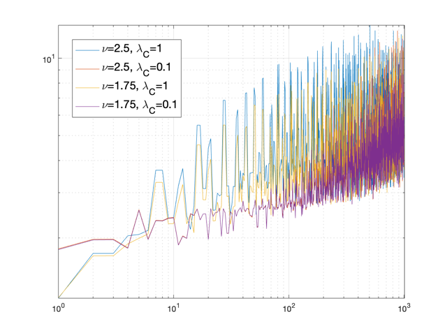
(a)

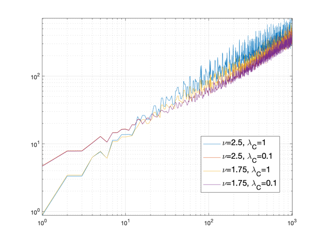
(b)

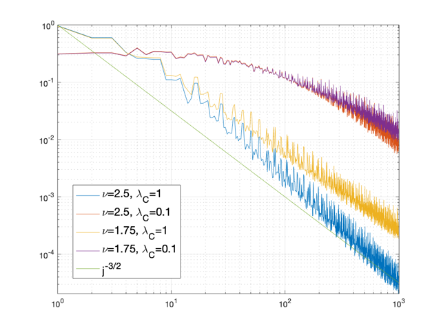
(c)

Figure 1: Log-log plot of $||\xi_{j}||_{\mathbb{C}^{0}(\overline{D})}$, $||\nabla\xi_{j}||_{\mathbb{C}^{0}(\overline{D})}$ and $b_{j}$ against $j$ for the Matérn covariance with $\nu=2.5$, $\sigma^{2}=1$, $\lambda_{C}=1$ in two dimension.

Next, we apply the component-by-component algorithm [42] to identify the generating vector $\boldsymbol{z}\in\mathbb{Z}^{s}$ for the randomly-shifted lattice rule with $N\in\mathbb{N}$ sampling points. To this end, we construct weighted Sobolev space $\mathcal{W}_{s}$ using the norm in (5.20). We choose the weight parameters $\gamma_{\boldsymbol{\mathfrak{u}}}$ according to (5.34), and the weight function $\psi^{2}_{j}(y)$ in (5.21). We choose $a_{j}=\sqrt{\frac{2\lambda_{*}-1}{8\lambda_{*}}}$ from (5.9), and the specific $\lambda_{\ast}$ depends on the empirical estimate $p$ we obtained from previous step. And we will choose different $\lambda_{\ast}$ according to different parameters.

Let us further choose $R=32$ independent random shifts as in (5.2), with each sample $\boldsymbol{\Delta}_{r}$ for $1\leq r\leq R$ being uniformly distributed over $[0,1]^{s}$. Subsequently, we can obtain the $N$ sampling points using the generator vector $\boldsymbol{z}\in\mathbb{Z}^{s}$,

$$\left(\frac{i\mathbb{z}}{N}+\boldsymbol{\Delta}_{r}\right)\bmod 1\text{ for all}1\leq i\leq N.$$

Given a certain quantity of interest defined by the linear functional $\mathcal{G}\in(L^{2}(D)^{2})^{\prime}$, We compute the quantity of interest $Q_{r}:=\mathcal{Q}_{s,N}(F^{J}_{s,h};\boldsymbol{\Delta_{r}})$, and its mean $\bar{Q}$ over $R$ random shifts. Then we have the following unbiased estimator for the root-mean-square error,

$$\sqrt{\frac{1}{R}\frac{1}{R-1}\sum_{r=1}^{R}(Q_{r}-\bar{Q})^{2}}\approx\sqrt{\mathbb{E}^{\boldsymbol{\Delta}}\left[\left(\mathbb{E}\left[\mathcal{G}(\boldsymbol{u}^{J}_{s,h})\right]-\mathcal{Q}_{s,N}(F^{J}_{s,h};\boldsymbol{\Delta})\right)^{2}\right]}.$$ (6.2)

The left-hand side of (6.2) is the so-called standard error.

To start with, we choose two specific bounded linear functional $\mathcal{G}$ as follows. The first bounded linear functional $\mathcal{G}_{1}$ is the first component of the point evaluation at $[1/2,1/2]$ when $t=0.1$, and the second one $\mathcal{G}_{2}$ is the second component of the point evaluation at $[1/2,1/2]$ when $t=0.2$. We also denote $\text{Error}1$ and $\text{Error}2$ as the standard error (6.2) corresponding to different linear functionals $\mathcal{G}_{1}$ and $\mathcal{G}_{2}$, respectively.

We first consider Matérn covariance with a smoothing parameter $\nu=2.5$, length scale parameter $\lambda_{C}=1$ and variance of $\sigma^{2}=1$ or $\sigma^{2}=0.25$. We observe numerically that the sequence $\{b_{j}\}_{j=1}^{\infty}$ lies under the sequence $\{j^{-3/2}\}_{j=1}^{\infty}$ for sufficiently large $j$. Therefore, we deduce empirically that Assumption 2.4 holds with some $p\leq 2/3$. Consequently, we take $\lambda_{\ast}:=0.55$ for those two cases.

N	$\sigma^{2}=1$				$\sigma^{2}=0.25$
	QMC		MC		QMC		MC
	Error1	Error2	Error1	Error2	Error1	Error2	Error1	Error2
1009	6.36e-04	4.65e-05	1.78e-03	1.68e-04	7.90e-05	8.60e-06	4.19e-04	3.23e-05
2003	3.77e-04	6.00e-05	1.61e-03	1.14e-04	2.92e-05	4.53e-06	2.99e-04	2.06e-05
4001	3.79e-04	5.80e-05	9.21e-04	1.17e-04	2.85e-05	4.17e-06	2.27e-04	1.77e-05
8009	1.79e-04	3.03e-05	5.76e-04	5.22e-05	1.04e-05	2.18e-06	1.22e-04	1.30e-05
16001	1.23e-04	1.12e-05	4.21e-04	3.34e-05	1.32e-05	8.40e-07	8.50e-05	6.66e-06
32003	6.24e-05	1.20e-05	2.32e-04	2.24e-05	8.60e-06	7.55e-07	6.05e-05	5.05e-06
64007	4.31e-05	7.90e-06	1.81e-04	1.79e-05	2.25e-06	1.76e-07	4.84e-05	4.55e-06
Rate	0.66	0.52	0.59	0.57	0.72	0.87	0.55	0.50

Table 1: Comparison of the standard error of QMC and MC with $\mathcal{G}_{1}$ and $\mathcal{G}_{2}$ for Matérn covariance with $\nu=2.5$, $\lambda_{C}=1$ and different $\sigma^{2}$.

In Table 1, we compare the standard error of QMC with MC for different linear functionals $\mathcal{G}_{1}$ and $\mathcal{G}_{2}$. To have a more precise estimate, for each number of sampling points $N$, we use the mean of ten different tests, using different uniformly distributed random shift ${\boldsymbol{\Delta}}$ in (5.2), as the quantity of interest. The rate is estimated together with the mean of ten tests by linear regression of the negative log of the standard error against $\log N$. We observe that QMC method results in a smaller error for both cases, and a faster convergence rate. For example, the standard error for QMC and MC are $4.31e-5$ and $1.81e-4$ with the number of sampling points $N=64007$ and variance $\sigma^{2}=1$.

For the case of $\lambda_{C}=0.1$, the empirical parameter $p$ has the value of $0.6832$, and hence we choose $\lambda_{*}=0.52$, which is presented in Table 2. One can observe similar performance as in Table 1. Due to the limitation of our computational resources, we can only perform our compuation up to $N=64007$. We note that we might have a better and more precise rate for larger number of sampling points.

N	$\sigma^{2}=1$				$\sigma^{2}=0.25$
	QMC		MC		QMC		MC
	Error1	Error2	Error1	Error2	Error1	Error2	Error1	Error2
1009	1.76e-03	8.26e-05	1.92e-03	1.68e-04	1.56e-04	1.42e-05	6.09e-04	5.79e-05
2003	1.14e-03	6.82e-05	3.81e-03	2.62e-04	8.88e-05	1.24e-05	1.22e-03	8.23e-05
4001	4.00e-04	3.80e-05	3.37e-03	1.33e-04	6.66e-05	6.85e-06	1.00e-03	3.87e-05
8009	3.91e-04	2.61e-05	1.33e-03	1.31e-04	3.07e-05	2.07e-06	4.20e-04	3.51e-05
16001	2.18e-04	1.96e-05	1.30e-03	6.77e-05	2.12e-05	1.81e-06	3.31e-04	2.27e-05
32003	1.66e-04	1.03e-05	7.99e-04	5.10e-05	2.21e-05	1.68e-06	2.63e-04	1.67e-05
64007	9.53e-05	8.67e-06	7.14e-04	4.33e-05	7.97e-06	7.72e-07	2.33e-04	1.33e-05
Rate	0.68	0.58	0.36	0.41	0.66	0.73	0.36	0.42

Table 2: Comparison of the standard error of QMC and MC with $\mathcal{G}_{1}$ and $\mathcal{G}_{2}$ for Matérn covariance with $\nu=2.5$, $\lambda_{C}=0.1$ and different $\sigma^{2}$.

Next we consider Matérn covariance with smoothing parameter $\nu=1.75$, length scale parameter $\lambda_{C}=1$ or $\lambda_{C}=0.1$, and variance of $\sigma^{2}=1$ or $\sigma^{2}=0.25$, respectively. Similar to the previous cases, the empirical parameter $p=0.7198$ when $\lambda_{C}=1$. This leads to $\lambda_{\ast}:=0.56$. For the case of $\lambda_{C}=0.1$, we estimate that the empirical parameter $p$ takes value of $0.8988$ and accordingly, we choose the parameter $\lambda_{\ast}=0.81$. The numerical results of QMC scheme using these parameters compared with MC are presented in Table 3 and Table 4.

N	$\sigma^{2}=1$				$\sigma^{2}=0.25$
	QMC		MC		QMC		MC
	Error1	Error2	Error1	Error2	Error1	Error2	Error1	Error2
1009	7.09e-04	1.06e-04	1.61e-03	2.35e-04	7.32e-05	1.14e-05	3.66e-04	4.96e-05
2003	4.69e-04	5.47e-05	1.59e-03	1.42e-04	7.53e-05	6.66e-06	3.57e-04	2.79e-05
4001	2.93e-04	3.85e-05	7.29e-04	8.35e-05	2.42e-05	3.01e-06	1.91e-04	1.99e-05
8009	1.78e-04	2.85e-05	5.14e-04	7.16e-05	1.97e-05	1.68e-06	1.39e-04	1.65e-05
16001	1.91e-04	1.78e-05	5.12e-04	5.37e-05	1.16e-05	1.48e-06	1.14e-04	1.26e-05
32003	1.15e-04	1.03e-05	5.90e-04	3.70e-05	8.98e-06	6.44e-07	1.27e-04	7.45e-06
64007	6.77e-05	6.08e-06	3.29e-04	2.67e-05	4.34e-06	5.32e-07	8.80e-05	8.31e-06
Rate	0.53	0.65	0.37	0.50	0.69	0.75	0.35	0.44

Table 3: Comparison of the standard error of QMC and MC with $\mathcal{G}_{1}$ and $\mathcal{G}_{2}$ for Matérn covariance with $\nu=1.75$, $\lambda_{C}=1$ and different $\sigma^{2}$.

N	$\sigma^{2}=1$				$\sigma^{2}=0.25$
	QMC		MC		QMC		MC
	Error1	Error2	Error1	Error2	Error1	Error2	Error1	Error2
1009	1.76e-03	9.78e-05	2.73e-03	2.01e-04	2.12e-04	9.82e-06	8.70e-04	6.65e-05
2003	7.76e-04	7.40e-05	3.24e-03	2.57e-04	1.19e-04	1.03e-05	1.14e-03	8.00e-05
4001	3.78e-04	3.73e-05	3.30e-03	9.66e-05	5.05e-05	3.67e-06	1.02e-03	3.33e-05
8009	4.54e-04	3.60e-05	1.11e-03	9.13e-05	6.07e-05	2.68e-06	3.74e-04	3.04e-05
16001	9.48e-05	1.50e-05	8.76e-04	6.76e-05	1.67e-05	2.03e-06	2.42e-04	2.14e-05
32003	9.23e-05	8.54e-06	8.32e-04	5.82e-05	1.36e-05	7.56e-07	2.65e-04	1.76e-05
64007	1.11e-04	6.32e-06	5.22e-04	3.62e-05	7.13e-06	6.23e-07	1.95e-04	1.21e-05
Rate	0.72	0.69	0.47	0.44	0.81	0.73	0.46	0.44

Table 4: Comparison of the standard error of QMC and MC with $\mathcal{G}_{1}$ and $\mathcal{G}_{2}$ for Matérn covariance with $\nu=1.75$, $\lambda_{C}=0.1$ and different $\sigma^{2}$.

Finally, we summarize all the numerical experiments from Table 1 to Table 4 and illustrate their convergence in Figure 2. One can observe a much smaller standard error for our proposed QMC method than the MC method for all cases. Furthemore, our proposed QMC method demonstrates a faster convergence rate for most of the cases.

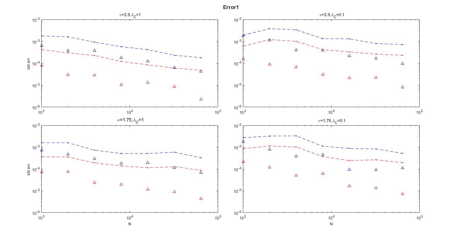
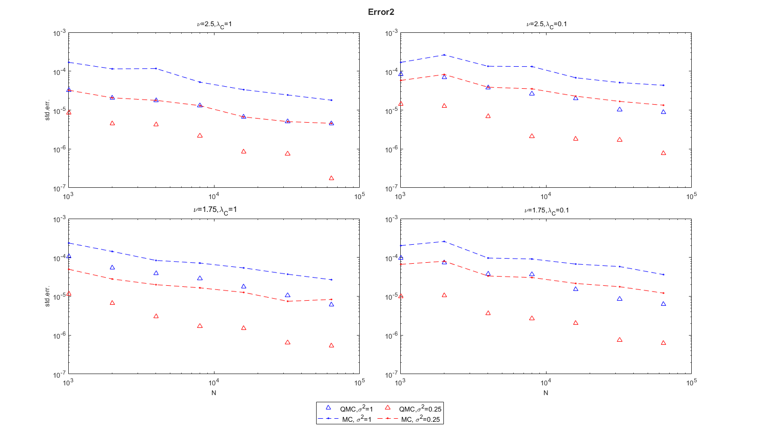
Figure 2: Standard errors for Error1 and Error2 with various Matérn covariance parameters for QMC and MC plotted against the number of sampling points $N$.

7 Conclusion

In this paper, we considered the Navier–Stokes equations with random initial data in a bounded polygonal domain $D\subset\mathbb{R}^{2}$. We have discussed an approximation scheme to compute the expectation value of the corresponding solution which combines the QMC method with the finite element method, the method that achieves a faster convergence rate compared with the classical MC method. Let us first summarize the theoretical results proved in the previous sections. In order to obtain a computable approximation of $\mathbb{E}[\mathcal{G}(\boldsymbol{u}(t_{J}))]$, we first truncate the KL expansion of the given initial data modeled by log-normal random fields. We then, for each realization $\boldsymbol{y}\in U_{\boldsymbol{b}}$, solve the corresponding Navier–Stokes system in $D$ based on the fully-implicit conforming Galerkin finite element method. We finally compute the expectation value of the resulting solution $\boldsymbol{u}^{J}_{s,h}$ by using the randomly-shifted QMC quadrature rule. Hence, our combined bound for the root-mean-square error consists of the finite element error, the dimension truncation error and the error for the QMC quadrature. More precisely, we may decompose the total error as

$$\mathbb{E}\left[\mathcal{G}(\boldsymbol{u}(t_{J}))\right]-\mathcal{Q}_{s,N}(F^{J}_{s,h};\boldsymbol{\Delta})$$

$$=\mathbb{E}\left[\mathcal{G}(\boldsymbol{u}(t_{J}))-\mathcal{G}(\boldsymbol{u}^{J}_{h})\right]+\mathbb{E}\left[\mathcal{G}(\boldsymbol{u}^{J}_{h})-\mathcal{G}(\boldsymbol{u}^{J}_{s,h})\right]+\left(\mathbb{E}\left[\mathcal{G}(\boldsymbol{u}^{J}_{s,h})\right]-\mathcal{Q}_{s,N}(F^{J}_{s,h};\boldsymbol{\Delta})\right),$$

where the expectation $\mathbb{E}$ above can be understood as the integral with respect to $\boldsymbol{y}\in U_{\boldsymbol{b}}$. The mean-square error with respect to the random shift $\boldsymbol{\Delta}$ then can be bounded by

$$\mathbb{E}^{\boldsymbol{\Delta}}\left[\left(\mathbb{E}[\mathcal{G}(\boldsymbol{u}(t_{J}))]-\mathcal{Q}_{s,N}(F^{J}_{s,h};\boldsymbol{\Delta})\right)^{2}\right]$$

$$\leq 3\left(\mathbb{E}\left[\mathcal{G}(\boldsymbol{u}(t_{J}))-\mathcal{G}(\boldsymbol{u}^{J}_{h})\right]\right)^{2}+3\left(\mathbb{E}\left[\mathcal{G}(\boldsymbol{u}^{J}_{h})-\mathcal{G}(\boldsymbol{u}^{J}_{s,h})\right]\right)^{2}+3\mathbb{E}^{\boldsymbol{\Delta}}\left[\left(\mathbb{E}\left[\mathcal{G}(\boldsymbol{u}^{J}_{s,h})\right]-\mathcal{Q}_{s,N}(F^{J}_{s,h};\boldsymbol{\Delta})\right)^{2}\right],$$

where each error on the right-hand side was estimated in Section 3, Section 4 and Section 5 in order. We present the combined error analysis discussed above in the following theorem.

Theorem 7.1.

Under the same assumptions and with the same definitions as in Theorem 3.5, Theorem 4.1 and Theorem 5.8, the root-mean-square error with respect to the random shift $\boldsymbol{\Delta}\in[0,1]^{s}$ can be estimated by

$$\sqrt{\mathbb{E}^{\boldsymbol{\Delta}}\left[\left(\mathbb{E}[\mathcal{G}(\boldsymbol{u}(t_{J}))]-\mathcal{Q}_{s,N}(F^{J}_{s,h};\boldsymbol{\Delta})\right)^{2}\right]}\leq C\left(t_{J}^{-\frac{1}{2}}h^{2}+\Delta t+s^{-\frac{k}{2}+1}+N^{-\chi}\right),$$ (7.1)

where for arbitrary $\delta\in(0,1/2]$,

$$\chi=\begin{cases}{-(1-\delta)}\quad&{\rm{if}}\,\,p\in(0,2/3],\\ {-(1/p-1/2)}\quad&{\rm{if}}\,\,p\in(2/3,1),\\ {-\frac{1}{2}}\quad&{\rm{if}}\,\,p=1\,\,{\rm{and}}\,\,\eqref{thm_further_ass}\,\,{\rm{holds}},\end{cases}$$

and where the constant $C>0$ is independent of $h,\Delta t>0$ and $s,N\in\mathbb{N}$.

To the best of our knowledge, the present paper is the first theoretical QMC analysis for the non-linear PDE. The main difficulty for the nonlinearity comes from the regularity of the solution with respect to the stochastic variable, which was analyzed in Theorem 5.2. Based on the argument used in this paper, one interesting future research topic is to cover a more general class of PDEs with a similar analysis. One particular topic of interest is to extend this result to the case of non-Newtonian fluid flow models, which describe the motion of fluids with more general structure [40, 41]. For this purpose, however, we need to find a new way to control the fully non-linear diffusion term, and the analysis for the corresponding convective term should be performed more carefully.

On the other hand, from the algorithmic point of view, it would be of independent interest to consider the multilevel and/or changing dimension algorithms [25, 37, 43, 44], with the QMC algorithm applied to the PDE problems with random data [34, 6, 31, 9]. Applying these analyses to the Navier–Stokes problem would be an intriguing future research topic.

References

[1]
G. A. Baker, V. A. Dougalis, and O. A. Karakashian.
On a higher order accurate fully discrete Galerkin approximation to
the Navier-Stokes equations.
Math. Comp., 39(160):339–375, 1982.
[2]
V. I. Bogachev.
Gaussian measures, volume 62 of Mathematical Surveys and
Monographs.
American Mathematical Society, Providence, RI, 1998.
[3]
R. E. Caflisch.
Monte Carlo and quasi-Monte Carlo methods.
In Acta numerica, 1998, volume 7 of Acta Numer., pages
1–49. Cambridge Univ. Press, Cambridge, 1998.
[4]
R. Cools, F. Y. Kuo, and D. Nuyens.
Constructing embedded lattice rules for multivariable integration.
SIAM J. Sci. Comput., 28(6):2162–2188, 2006.
[5]
J. Dick.
On the convergence rate of the component-by-component construction of
good lattice rules.
J. Complexity, 20(4):493–522, 2004.
[6]
J. Dick, F. Y. Kuo, Q. T. Le Gia, and C. Schwab.
Multilevel higher order QMC Petrov-Galerkin discretization for
affine parametric operator equations.
SIAM J. Numer. Anal., 54(4):2541–2568, 2016.
[7]
J. Dick, F. Y. Kuo, and I. H. Sloan.
High-dimensional integration: the quasi-Monte Carlo way.
Acta Numer., 22:133–288, 2013.
[8]
J. Dick, F. Pillichshammer, and B. J. Waterhouse.
The construction of good extensible rank-1 lattices.
Math. Comp., 77(264):2345–2373, 2008.
[9]
M. B. Giles, F. Y. Kuo, and I. H. Sloan.
Combining sparse grids, multilevel MC and QMC for elliptic PDEs
with random coefficients.
In Monte Carlo and quasi–Monte Carlo methods, volume 241
of Springer Proc. Math. Stat., pages 265–281. Springer, Cham, 2018.
[10]
V. Girault and P.-A. Raviart.
Finite element methods for Navier-Stokes equations,
volume 5 of Springer Series in Computational Mathematics.
Springer-Verlag, Berlin, 1986.
Theory and algorithms.
[11]
I. G. Graham, F. Y. Kuo, J. A. Nichols, R. Scheichl, C. Schwab, and I. H.
Sloan.