Training Graph Neural Networks on Growing Stochastic Graphs

Abstract

Graph Neural Networks (GNNs) rely on graph convolutions to exploit meaningful patterns in networked data. Based on matrix multiplications, convolutions incur in high computational costs leading to scalability limitations in practice. To overcome these limitations, proposed methods rely on training GNNs in smaller number of nodes, and then transferring the GNN to larger graphs. Even though these methods are able to bound the difference between the output of the GNN with different number of nodes, they do not provide guarantees against the optimal GNN on the very large graph. In this paper, we propose to learn GNNs on very large graphs by leveraging the limit object of a sequence of growing graphs, the graphon. We propose to grow the size of the graph as we train, and we show that our proposed methodology – learning by transference – converges to a neighborhood of a first order stationary point on the graphon data. A numerical experiment validates our proposed approach.

Index Terms—  Graph Neural Networks, Graphons

1 Introduction

Graph Neural Networks (GNNs) are deep convolutional architectures for non-Euclidean data supported on graphs [1, 2]. GNNs are formed by a succession of layers, each of which is composed of a graph convolutional filter and a point-wise non-linearity. In practice, GNNs have shown state-of-the-art performance in several learning tasks [3, 4], and have found applications in biology [5, 6, 7], recommendation systems [8, 9, 10] and robotics [11, 12]. In theory, part of their success is credited to their stability to graph perturbations [2], the fact that they are invariant to relabelings [13, 14], their expressive power [15, 16], and their generalization capabilities [17].

The ability of GNNs to exploit patterns in network data is largely due to their graph convolutional layers. Graph convolutional filters leverage the graph diffusion sequence to extract features that are shared across the graph [2]. However, these filters rely on computing matrix-vector multiplications, which become computationally costly when the number of nodes is large. On the other hand, the number of parameters in a GNN is independent of the number of nodes due to its local parametrization, which motivates training GNNs on small graphs and then deploying them on larger graphs.

Several works have been proposed which exploit this transferability property of the GNN [18, 19, 20]. Generally speaking, these works upper bound the output difference between two GNNs with the same parameters supported on graphs with different number of nodes. They show that if the graphs belong to a family of graphs modeled by a graphon [21], as the number of nodes increases the so-called transferability error decreases. But while this result is useful, it does not guarantee than the optimal parameters achieved by training the GNN on the small graph are optimal, or sufficiently close to optimal, on the large graph. This subtle albeit crucial observation is what motivates our work.

More specifically, we leverage the transferability properties of GNNs to introduce a method that trains GNNs by successively increasing the size of the graph during the training process. We call this procedure learning by transference. We prove that the learning directions (gradients) on the graphon and on the graph are aligned as long as the number of nodes in the GNN is sufficiently large. Under a minimum graph size at each epoch, we show that our method converges to a neighborhood of the first order stationary point on graphon by taking gradient steps on the graph. We benchmark our procedure in a multi-agent system problem, where a GNN is trained to learn a decentralized control policy for agents communicating via a proximity graph.

Related work. This work extends upon previous works that consider the nodes to be sampled from a regular partition of the graphon [22]. In this work, we consider the nodes to be uniformly sampled, which not only provides a more general modeling of GNNs, but also more closely correlates with graph signals seen in practice. This more general sampling strategy induces further sampling errors (in addition to the edge sampling error) [19], which worsen the approximation of graphons and graphon data by graphs and graph data thus requiring additional theoretical considerations.

2 Graph and Graphon Neural Networks

A graph is represented by the triplet ${\mathbf{G}}_{n}=({\mathcal{V}},{\mathcal{E}},W)$, where ${\mathcal{V}},|{\mathcal{V}}|=n$ is the set of nodes, ${\mathcal{E}}\subseteq{\mathcal{V}}\times{\mathcal{V}}$ is the set of edges, and $W:{\mathcal{E}}\to{\mathbb{R}}$ is a map assigning weights to each edge. Alternatively, we can represent the graph ${\mathbf{G}}_{n}$ by its graph shift operator (GSO) ${\mathbf{S}}_{n}\in{\mathbb{R}}^{n\times n}$. Examples of GSO are the adjecency matrix ${\mathbf{A}}$, the graph laplacian ${\mathbf{L}}=\mbox{diag}({\mathbf{A}}{\mathbf{1}})-{\mathbf{A}}$, to name a few.

Data on graphs is defined as a graph signal ${\mathbf{x}}=[x_{1},\dots,x_{n}]$, where the $i$th component of ${\mathbf{x}}$ corresponds to the value of the signal on node $i$. A graph signal ${\mathbf{x}}$ can be aggregated through the graph, by applying the GSO ${\mathbf{S}}_{n}$ as follows,

$${\mathbf{z}}={\mathbf{S}}_{n}{\mathbf{x}}_{n}.$$ (1)

Intuitively, the value of signal ${\mathbf{z}}$ at coordinate $i$ is the weighted average of the information present in its one hop neighborhood, i.e. $z_{i}=\sum_{j\in{\mathcal{N}}(i)}[{\mathbf{S}}_{n}]_{ij}x_{j}$. We can construct $k$-hop diffusion by applying $k$ power of ${\mathbf{S}}_{n}$. We define the graph convolutions, as a weighted average over the powers of ${\mathbf{S}}_{n}$. Explicitly, by letting the coefficients be ${\mathbf{h}}=[h_{0},\dots,h_{K-1}]$, we define the graph convolution as,

$${\mathbf{y}}_{n}={\mathbf{h}}_{*{\mathbf{S}}_{n}}{\mathbf{x}}_{n}=\sum_{k=0}^{K-1}h_{k}{\mathbf{S}}_{n}^{k}{\mathbf{x}}_{n}$$ (2)

where ${\mathbf{x}}_{n},{\mathbf{y}}_{n}$ are graph signals, and ${\mathbf{h}}_{*{\mathbf{S}}_{n}}$ denotes the convolution operator with GSO ${\mathbf{S}}_{n}$.

In the case of undirected graphs, ${\mathbf{S}}_{n}/n$ becomes symmetric, admitting a spectral decomposition ${\mathbf{S}}_{n}={\mathbf{V}}\boldsymbol{\Lambda}{\mathbf{V}}^{T}$, where the columns of ${\mathbf{V}}$ are the eigenvectors of ${\mathbf{S}}_{n}$, and $\boldsymbol{\Lambda}$ is a diagonal matrix with $-1\leq\dots\leq\dots 1$. Since the eigenvector of ${\mathbf{S}}_{n}$ for a basis of ${\mathbb{R}}^{n}$, we can project filter ${\mathbf{y}}_{n}$ into this basis to obtain,

$$h(\lambda)=\sum_{k=0}^{K-1}h_{k}\lambda^{k}$$ (3)

Note that $h(\lambda)$ only depends on $h_{k}$, and on the eigenvalues of the GSO. By the Cayley-Hamilton theorem, convolutional filters may be used to represent any graph filter with spectral representation $h(\lambda)=f(\lambda)$, where $f$ is analytic.

Graph Neural Networks are layered architectures, composed of graph convolutions followed by point-wise non-linearities. Formally, introducing a point-wise non-linearity $\rho$, and by stacking all the graph signals at layer $l$ in a matrix ${\mathbf{X}}_{l}=[{\mathbf{x}}_{nl}^{1},\dots,{\mathbf{x}}_{nl}^{F_{l}}]\in{\mathbb{R}}^{n\times F_{l}}$, where $F_{l}$ indicates the $F_{l}$ features at layer $l$. Notice that for $l=0$, the input matrix is a concatenation of the input signal, i.e. ${\mathbf{X}}_{0}=[{\mathbf{x}}_{n},\dots,{\mathbf{x}}_{n}]$. We can define the $l$ layer of a GNN as,

$${\mathbf{X}}_{l}=\rho\bigg{(}\sum_{k=1}^{K}{\mathbf{X}}_{n}^{k}{\mathbf{X}}_{l_{1}}{\mathbf{H}}_{lk}\bigg{)},$$ (4)

where matrix ${\mathbf{H}}_{lk}\in{\mathbb{R}}^{F_{l-1}\times F_{l}}$ represents the $k$ coefficient of the graph convolution. By grouping all the learnable parameters we can obtain a more succint representation of the GNN as $\phi({\mathbf{x}};{\mathcal{H}},{\mathbf{S}})$, with ${\mathcal{H}}=\{{\mathbf{H}}_{lk}\}_{lk},1\leq l\leq L$, and $0\leq k\leq K-1$.

2.1 Graphon Neural Networks

Graphons are the limit object of a converging sequence of dense undirected graphs. Formally, a graphon is a symmetric, bounded, and measurable function ${\mathbf{W}}:[0,1]^{2}\to[0,1]$. Sequences of dense graphs converge to a graphon in the sense that the densities of adjacency preserving graph motifs converge to the densities of these same motifs on the graphon [18, 21].

Analogously to graph signals, we can define a graphon signal as a function $X\in L^{2}([0,1])$. A graphon signal can be diffused over the graphon by applying the linear integrator operator given by,

$$T_{\mathbf{W}}X(v)=\int_{0}^{1}{\mathbf{W}}(u,v)X(v)du$$ (5)

which we denote graphon shift operator (WSO). Since graphon ${\mathbf{W}}$ is bounded and symmetric, $T_{\mathbf{W}}$ is a Hilbert-Schmidt and self adjoint operator [23]. Therefore, we can express ${\mathbf{W}}$ by its eigen decomposition, ${\mathbf{W}}(u,v)=\sum_{i\in{\mathbb{Z}}\smallsetminus 0}\lambda_{i}\phi_{i}(u)\phi_{i}(v)$, where $\lambda_{i}$ is the eigenvalue associated with eigenfunction $\phi_{i}$. The absolute value of the eigenvalues is bounded by $1$, and the eigenfunctions form an orthogonal basis of $L^{2}([0,1])$. Utilizing the graphon shift, we define the graphon convolution with parameters ${\mathbf{h}}=[h_{0},\dots,h_{K-1}]$, as

$$Y=T_{\mathbf{h}}X={\mathbf{h}}_{*{\mathbf{W}}}X=\sum_{k=0}^{K-1}h_{k}(T_{\mathbf{W}}^{(k)}X)(v)\text{ with }$$ (6)

$$(T_{\mathbf{W}}^{(k)}X)(v)=\int_{0}^{1}{\mathbf{W}}(u,v)(T_{\mathbf{W}}^{(k-1)}X)(u)du$$ (7)

where $X,Y$ are graphon signals, $*{\mathbf{W}}$ defines the convolution operator, and $T^{(0)}={\mathbf{I}}$ is the identity[24]. Projecting the filter (6) onto the eigenbasis $\{\phi_{i}\}_{i\in{\mathbb{Z}}\smallsetminus 0}$, the graphon convolution admits a spectral representation given by,

$$h(\lambda)=\sum_{k=0}^{K-1}h_{k}\lambda^{k}.$$ (8)

Like its graphon counterpart (cf. (3)) the graphon convolution admits a spectral representation that only depends on the coefficients of the filter ${\mathbf{h}}$.

Graphon Neural Networks (WNNs) are the extension of GNNs to graphon data. Each layer of a WNN is composed by a graphon convolution (6), and a non-linearity $\rho$. Denoting $F_{l}$ the features at layer $l$, we can group the parameters of the $F_{l-1}\times F_{l}$ convolutions into $K$ matrices $\{{\mathbf{H}}_{lk}\}\in{\mathbb{R}}^{F_{l-1}\times F_{l}}$, to write the $f$ th feature of the $l$th layer as follows,

$$X_{l}^{f}=\rho\bigg{(}\sum_{g=1}^{F_{l-1}}\sum_{k=1}^{K-1}(T_{\mathbf{W}}^{(k)}X_{l-1}^{g})[{\mathbf{H}}_{lk}]_{gf}\bigg{)}$$ (9)

for $1\leq g\leq F_{0}$. For an $L$ layered WNN, $X_{0}^{g}$ is given by the input data $X^{g}$, and (9) is repeated for $1\leq l\leq L$, and the output of the WNN is given by $Y=X_{L}$. Analogoues to GNNS, a more succint representation of the WNN can be obtained be grouping all the coefficients, i.e. $\phi(X;{\mathcal{H}},{\mathbf{W}})$, with ${\mathcal{H}}=\{{\mathbf{H}}_{lk}\}_{lk},1\leq l\leq L$, and $0\leq k\leq K-1$.

2.2 From Graphons to Graphs, and Back

In this paper we focus on graphons, and graphon signals as generative models of graphs, and graph signals. Let $\{u_{i}\}_{i=1}^{N}$ be $n$ points sampled independently at uniformly from $[0,1]$, $u_{i}\sim\text{unif}(0,1)$. The $n$-node stochastic GSO of graph ${\mathbf{G}}_{n}$ is obtained from graphon ${\mathbf{W}}$ as follows,

$$[{\mathbf{S}}_{n}]_{ij}=[{\mathbf{S}}_{n}]_{ji}\sim\text{Bernoulli}({\mathbf{W}}(u_{i},u_{j})))$$ (10)

A graph signal ${\mathbf{x}}$ can be obtained by evaluating the graphon signal,

$$[{\mathbf{x}}]_{i}=X(u_{i})\text{ for all }i\in[n].$$ (11)

Therefore, we can obtain stochastic graphs ${\mathbf{S}}_{n}$, and graph signals ${\mathbf{x}}$ from graphon data ${\mathbf{W}},X$.

A graphon can be induced by a graph even if the node labels $\{u_{i}\}_{i=1}^{N}$ are unknown. Let ${\mathbf{S}}_{n}\in{\mathbb{R}}^{n\times n}$ be the GSO of a graph, and define $u_{i}=(i-1)/n$ for $1\leq i\leq n$. We construct the intervals $I_{i}=[u_{i},u_{i+1}]$ for $1\leq i\leq n$. Letting ${\mathbf{1}}$ be the indicator function, the induced graphon ${\mathbf{W}}_{\mathbf{S}}$, and graph signal ${\mathbf{x}}$ can be obtained as,

$${\mathbf{W}}_{\mathbf{S}}(u,v) =\sum_{i=1}^{n}\sum_{j=1}^{n}[{\mathbf{S}}_{n}]_{ij}{\mathbf{1}}(u\in I_{i}){\mathbf{1}}(v\in I_{j}),\text{ and }$$ (12)

$$X_{n}(u) =\sum_{i=1}^{n}[{\mathbf{x}}_{n}]_{i}{\mathbf{1}}(u\in I_{i}).$$ (13)

Algorithm 1 Learning by transference

1:Initialize ${\mathcal{H}}_{0},n_{0}$ and sample graph ${\mathbf{G}}_{n_{0}}$ from graphon ${\mathbf{W}}$

2:repeat for epochs $0,1,\ldots$

3:     for $k$ =1,…, $|{\mathcal{D}}|$ do

4:         Obtain sample $(Y,X)\sim{\mathcal{D}}$

5:         Construct graph signals ${\mathbf{y}}_{n},{\mathbf{x}}_{n}$ [cf. (11)]

6:         Take learning step:

7:    ${\mathcal{H}}_{k+1}={\mathcal{H}}_{k}-\eta_{k}\nabla\ell({\mathbf{y}}_{n},\boldsymbol{\Phi}({\mathbf{x}}_{n};{\mathcal{H}}_{k},{\mathbf{S}}_{n}))$

8:     end for

9:     Increase number of nodes $n$

10:     Sample points uniformly $u_{i}\sim unif(0,1)$, $i=[1,\dots,n]$

11:     Sample ${\mathbf{S}}_{n}$ Bernoulli from graphon ${\mathbf{W}}$ [cf. (10)]

12:until convergence

3 Learning By Transference

We are interested in solving a statistical learning problem where the data is supported in very large graphs. In the limit, this corresponds to a graphon, so we consider the problem of learning a WNN.

Let $\ell:{\mathbb{R}}\times{\mathbb{R}}\to{\mathbb{R}}$ be a non-negative loss function such that $\ell(x,y)=0$ if and only if $x=y$, and let $p(X,Y)$ be an unknown probability distribution over the space of the graphon signal. The graphon statistical learning problem is defined as

$$\min_{{\mathcal{H}}}{\mathbb{E}}_{p(X,Y)}[\ell(Y,\phi(X;{\mathcal{H}},{\mathbf{W}}))].$$ (14)

Given that the joint probability distribution $p(X,Y)$ is unknown, a solution of 14 cannot be derived in close form but, under the learning paradigm, we assume that we have access to samples of the distribution ${\mathcal{D}}=\{(X^{j},Y^{j})\sim p(X,Y),j=1,\dots,|{\mathcal{D}}|\}$. Provided that the samples in ${\mathcal{D}}$ are obtained independently, and that $|{\mathcal{D}}|$ is sufficiently large, 14 can be approximated by its empirical version

$$\min_{{\mathcal{H}}}\frac{1}{|{\mathcal{D}}|}\sum_{j=1}^{|{\mathcal{D}}|}\ell(Y^{j},\phi(X^{j};{\mathcal{H}},{\mathbf{W}})).$$ (15)

Like most other empirical risk minimization problems, the graphon empirical learning problem (15) is solved in an iterative fashion by gradient descent. The $k$th gradient descent iteration is given by

$${\mathcal{H}}_{k+1}={\mathcal{H}}_{k}-\eta_{k}\frac{1}{|{\mathcal{D}}|}\sum_{j=1}^{|{\mathcal{D}}|}\nabla_{\mathcal{H}}\ell(Y^{j},\phi(X^{j};{\mathcal{H}}_{k},{\mathbf{W}}))$$ (16)

where $\eta_{k}\in(0,1)$ is the step size at iteration $k$.

In practice, however, the limit graphon ${\mathbf{W}}$ is either unknown or hard to measure, and step (16) cannot be computed. But this can be addressed by noting that this gradient can be approximated by sampling graphs ${\mathbf{S}}_{n}$ (cf. (16)) and computing the gradient descent iteration on the graph. Explicitly,

$${\mathcal{H}}_{k+1}={\mathcal{H}}_{k}-\eta_{k}\frac{1}{|{\mathcal{D}}|}\sum_{j=1}^{|{\mathcal{D}}|}\nabla_{\mathcal{H}}\ell({\mathbf{y}}^{j},\phi({\mathbf{x}}^{j};{\mathcal{H}}_{k},{\mathbf{S}}_{n})).$$ (17)

To show that the graphon (16) and the graph gradient descent iterations (17) are close, we need the following assumptions.

Definition 1 (Lipschitz Functions)

A function $f$ is $A$-Lipschitz on the variables $u_{1},\ldots,u_{d}$ if it satisfies $|f(v_{1},v_{2},\ldots,v_{d})-f(u_{1},u_{2},\ldots,u_{d})|\leq A\sum_{i=1}^{d}|v_{i}-u_{i}|$. If $A=1$, we say that this function is normalized Lipschitz.

Definition 2 (Node Stochasticity)

For a fixed probability ${\mathcal{X}}_{1}\in[0,1]$, the node stochasticity constant on $n$ nodes, denoted $\alpha({\mathcal{X}}_{1},n)$ is defined as $\alpha({\mathcal{X}}_{1},n)=\log((n+1)^{2}/\log(1-{\mathcal{X}}_{1})^{-1})$.

Definition 3 (Edge Stochasticity)

For a fixed probability ${\mathcal{X}}_{2}\in[0,1]$, the edge stochasticity constant on $n$ nodes, denoted $\beta({\mathcal{X}}_{2},n)$ is defined as $\beta({\mathcal{X}}_{2},n)=\sqrt{n\log(2n/{\mathcal{X}}_{2})}$.

AS 1

The graphon ${\mathbf{W}}$ and graphon signals $X,Y$ are normalized Lipschitz.

AS 2

The convolutional filters $h$ are normalized Lipschitz and non-amplifying, i.e., $\|h(\lambda)\|<1$.

AS 3

The activation functions and their gradients are normalized Lipschitz, and $\rho(0)=0$.

AS 4

The loss function $\ell:{\mathbb{R}}\times{\mathbb{R}}\to{\mathbb{R}}^{+}$ and its gradient are normalized Lipschitz, and $\ell(x,x)=0$.

AS 5

For a fixed value of ${\mathcal{X}}_{3}\in(0,1)$, $n$ is such that $n-{\log(2n/{\mathcal{X}}_{3})}/{d_{\mathbf{W}}}>{2}/{d_{\mathbf{W}}}$ where $d_{\mathbf{W}}$ denotes the maximum degree of the graphon ${\mathbf{W}}$, i.e., $d_{\mathbf{W}}=\max_{v}\int^{1}_{0}{\mathbf{W}}(u,v)du$.

Theorem 1

Consider the ERM problem in (15) and let $\boldsymbol{\Phi}(X;{\mathcal{H}},{\mathbf{W}})$ be an $L$-layer WNN with $F_{0}=F_{L}=1$, and $F_{l}=F$ for $1\leq l\leq L-1$. Let $c\in(0,1]$ and assume that the graphon convolutions in all layers of this WNN have $K$ filter taps [cf. (6)]. Let $\boldsymbol{\Phi}({\mathbf{x}}_{n};{\mathcal{H}},{\mathbf{S}}_{n})$ be a GNN sampled from $\boldsymbol{\Phi}(X;{\mathcal{H}},{\mathbf{W}})$ as in (10), and (11). Under assumptions AS1–AS5, it holds that

$${\mathbb{E}}[\|\nabla_{{\mathcal{H}}} \ell(Y,\phi(X;{\mathcal{H}},{\mathbf{W}}))-\nabla_{{\mathcal{H}}}\ell(Y_{n},\phi(X_{n};{\mathcal{H}},{\mathbf{W}}_{n}))\|]$$

$$\leq\gamma c+{\mathcal{O}}\bigg{(}\max(\alpha(1/\sqrt{n},n),\beta(1/\sqrt{n},n))\bigg{)}$$ (18)

where $Y_{n}$ is the graphon signal induced by $[{\mathbf{y}}_{n}]_{i}=Y(u_{i})$ [cf. (12)], and $\gamma=12\sqrt{K^{5}F^{5L-5}}$.

As expected, the bound in (1) decreases with the number of nodes, but it also contains a constant term called the non-transferable bound, which corresponds to high-frequency spectral components that converge more slowly with $n$ (see [19, Sec. IV.C]).

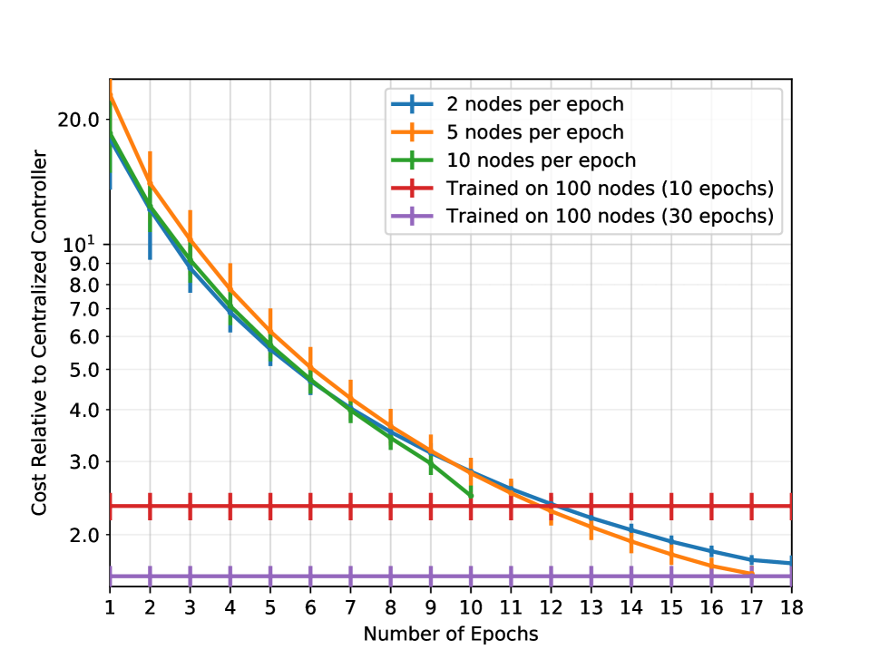
(a) Starting with $10$ nodes

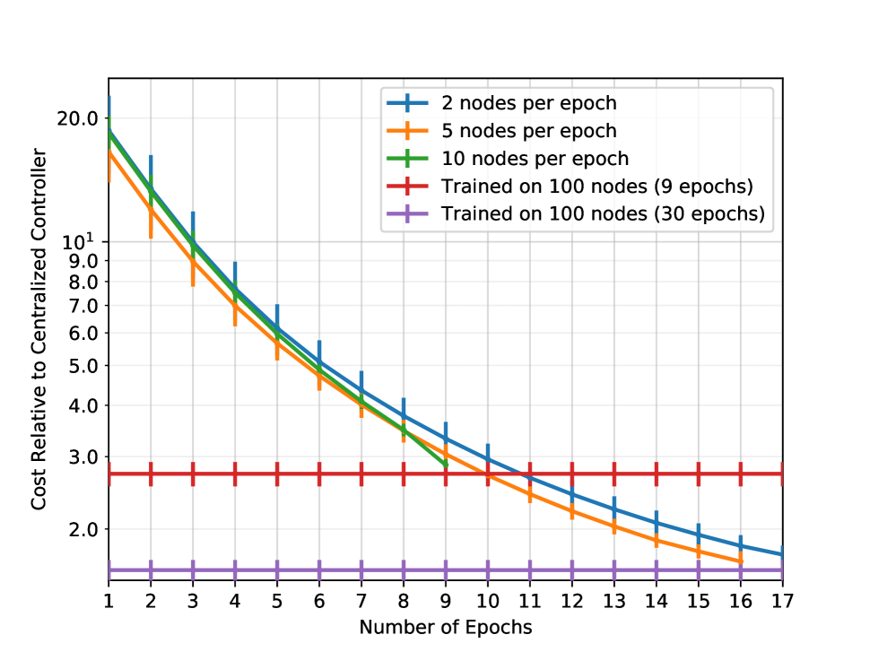
(b) Starting with $20$ nodes

Fig. 1: Velocity variation of the flocking problem for the whole trajectory in the testing set relative to the centralized controller.

3.1 Algorithm Construction

Algorithm 1 presents a simple strategy for training GNNs for large graphs: increasing the number of nodes and resampling the graph at regular intervals during the training process. The insight is that at the beginning of the learning process, the gradient on the graphon is large, given that the parameters ${\mathcal{H}}_{k}$ are distant from the optimal values. As we train, the norm of the gradient on the graphon decreases, and we require a larger graph, i.e., a better approximation of the graphon, to follow the right learning direction on the graph.

The advantage of Algorithm 1 versus training on the large $N$-node graph directly is that given that the convolutions implement matrix-vector multiplications, this would require ${\mathcal{O}}(N^{2})$ computations. By implementing Algorithm 1, we are able to bring this down to ${\mathcal{O}}(n^{2})$ computations, $n<N$, without compromising optimality. What is more, Algorithm 1 might not require evaluating gradients on the very large graph, as it could be the case that smaller graphs render the desired optimality conditions.

3.2 Algorithm Convergence

To show the convergence of Algorithm 1, we need additional Lipschitz assumptions.

AS 6

The graphon neural network $\boldsymbol{\Phi}(X;{\mathcal{H}},{\mathbf{W}})$ is ${A_{\boldsymbol{\Phi}}}$-Lipschitz, and its gradient $\nabla_{\mathcal{H}}\boldsymbol{\Phi}(X;{\mathcal{H}},{\mathbf{W}})$ is ${A_{\nabla\boldsymbol{\Phi}}}$-Lipschitz, with respect to the parameters ${\mathcal{H}}$ [cf. Definition 1].

Theorem 2

Consider the ERM problem in (15) and let $\boldsymbol{\Phi}(X;{\mathcal{H}},{\mathbf{W}})$ be an $L$-layer WNN with $F_{0}=F_{L}=1$, and $F_{l}=F$ for $1\leq l\leq L-1$. Let $c\in(0,1]$, $\epsilon>0$, step size $\eta<{{A_{\nabla\ell}}}^{-1}$, with ${A_{\nabla\ell}}={A_{\nabla\Phi}}+{A_{\boldsymbol{\Phi}}}F^{2L}\sqrt{K}$ and assume that the graphon convolutions in all layers of this WNN have $K$ filter taps [cf. (6)]. Let $\boldsymbol{\Phi}({\mathbf{x}}_{n};{\mathcal{H}},{\mathbf{S}}_{n})$ be a GNN sampled from $\boldsymbol{\Phi}(X;{\mathcal{H}},{\mathbf{W}})$ as in (12). Consider the iterates generated by equation (17), under Assumptions AS1-AS6, if at each step $k$ the number of nodes $n$ verifies

$${\mathbb{E}}[\|\nabla_{{\mathcal{H}}_{k}} \ell(Y,\boldsymbol{\Phi}(X;{\mathcal{H}}_{k},{\mathbf{W}}))-\nabla_{{\mathcal{H}}}\ell(Y_{n},\boldsymbol{\Phi}(X_{n};{\mathcal{H}},{\mathbf{W}}_{n}))\|]$$

$$+\epsilon<\|\nabla_{{\mathcal{H}}}\ell(Y,\boldsymbol{\Phi}(X;{\mathcal{H}}_{k},{\mathbf{W}}))\|$$ (19)

then Algorithm 1 converges to an $\epsilon$-neighborhood of the solution of the Graphon Learning problem (15) in at most $k^{*}={\mathcal{O}}(1/\epsilon^{2})$ iterations, with $\gamma=12\sqrt{K^{5}F^{5L-5}}$].

Theorem 2 provides the conditions under which Algorithm 1 converges to a neighborhood of the first order stationary point of the empirical graphon learning problem (15). Other than the aforementioned smoothness assumptions, we only need to satisfy condition (2) at every epoch, i.e., the norm of the gradient on the graphon has to be larger than the difference between the gradients on the graph and graphon.

4 Experiments

We consider the problem of coordinating the velocity of a set of $n$ agents while avoiding collisions. At each time $t$ each agents knows its own position $r(t)_{i}\in{\mathbb{R}}^{2}$, and speed $v(t)_{i}\in{\mathbb{R}}^{2}$, and reciprocally exchanges it with its neighbors. Communication links $[{\mathbf{S}}]_{ij}$ exists if the distance between two agents $i,j$ is smaller that $2$ meters. At each time $t$ the controller sets an acceleration that remains constant over an interval of $T_{s}=20ms$. The system dynamics is governed by,

$$r_{i}(t+1) =u_{i}(t)T_{s}^{2}/2+v_{i}(t)T_{s}+r_{i}(t),$$ (20)

$$v_{i}(t+1) =u_{i}(t)T_{s}+v_{i}(t).$$ (21)

We define the velocity variation of the team as $\sigma_{{\mathbf{v}}(t)}=\sum_{i=1}^{n}\|v_{i}(t)-\bar{\mathbf{v}}(t)\|^{2}$, and the collision avoidance potential

$$\begin{split}CA_{ij}=\begin{cases}\frac{1}{\|r_{i}-r_{j}\|^{2}}-\log(\|r_{i}-r_{j}\|^{2})&\text{if $\|r_{i}-r_{j}\|\leq R_{CA}$}\\ \frac{1}{R_{CA}^{2}}-\log(R_{CA}^{2})&\text{otherwise,}\end{cases}\end{split}$$

with $R_{CA}=1m$. We consider a centralized controller whose action is given by $u_{i}(t)^{*}=-n(v_{i}-\bar{\mathbf{v}})+\sum_{j=1}^{n}\nabla_{r_{i}}CA(r_{i},r_{j})$ [25].

The learning setting is created by training a GNN that mimics the output of the centralized controller. To do so, we define the empirical risk minimization problem over the dataset ${\mathcal{D}}=\{{\mathbf{u}}^{*}_{m},{\mathbf{x}}_{m}\}_{m}$ for $m\in[0,400]$,

$$\min_{\mathcal{H}}\sum_{m=1}^{|{\mathcal{D}}|}\|{\mathbf{u}}^{*}_{m}-\boldsymbol{\Phi}({\mathbf{x}}_{m};{\mathcal{H}},{\mathbf{S}})\|^{2}.$$ (22)

In Figure 1 we can see the velocity variation of the learned GNN measured on unseen data. Figure 1 validates the utility of the proposed method, as we are able to learn GNNs utilizing Algorithm 1 that achieve a comparable performance with the GNN trained on all the nodes. GNNs are that are trained with starting number of nodes $n_{0}=\{10,20\}$, and that add $10$ agents per epoch (green line) are able to achieve a similar performance when reaching $100$ agents than the one they would have achieved by training with $100$ agents the same number of epochs. This is the empirical manifestation of Theorem 2. Moreover, adding less agents per epoch (orange and blue lines) still achieve the same performance, but it takes more epochs to achieve. Overall, all the presented configurations are able to obtain a comparable performance that the one obtained with the full graph of $100$ agents while taking steps of graphs of growing sizes.

5 Conclusion

In this paper we presented a method for learning GNNs on very large graphs by growing the size of the graph as we train. Denoted learning by transference, we exploit the fact that the norm of the gradient on WNN decreases as it approaches a minima, and so we increase the precision at which we estimate it as epochs increase. We provide a proof of convergence of our algorithm, as well as numerical experiments on a multi-agent problem.

Appendix A Proof of Theorem 1

Theorem 2 follows directly from Theorem [22, Theorem $1$], and [22, Lemma $3$] with $\alpha$ as in the node stochasticity. It is also needs to be noted that ${\mathcal{X}}_{1}$, ${\mathcal{X}}_{2}$, and ${\mathcal{X}}_{3}$ should be selected as $\sqrt{n}$. The maximum in the final bound comes from fact that the bound is governed by the maximum rate between $\beta$, and $\alpha$.

Appendix B Proof of Theorem 2

See [22, Theorem $2$].

References

- [1] Thomas N Kipf and Max Welling, “Semi-supervised classification with graph convolutional networks,” arXiv preprint arXiv:1609.02907, 2016.
- [2] Fernando Gama, Antonio G Marques, Geert Leus, and Alejandro Ribeiro, “Convolutional neural network architectures for signals supported on graphs,” IEEE Transactions on Signal Processing, vol. 67, no. 4, pp. 1034–1049, 2018.
- [3] Yue Wang, Yongbin Sun, Ziwei Liu, Sanjay E Sarma, Michael M Bronstein, and Justin M Solomon, “Dynamic graph cnn for learning on point clouds,” Acm Transactions On Graphics (tog), vol. 38, no. 5, pp. 1–12, 2019.
- [4] Michael M Bronstein, Joan Bruna, Yann LeCun, Arthur Szlam, and Pierre Vandergheynst, “Geometric deep learning: going beyond euclidean data,” IEEE Signal Processing Magazine, vol. 34, no. 4, pp. 18–42, 2017.
- [5] Alex Fout, Jonathon Byrd, Basir Shariat, and Asa Ben-Hur, “Protein interface prediction using graph convolutional networks,” in Advances in Neural Information Processing Systems, I. Guyon, U. V. Luxburg, S. Bengio, H. Wallach, R. Fergus, S. Vishwanathan, and R. Garnett, Eds. 2017, vol. 30, Curran Associates, Inc.
- [6] David K Duvenaud, Dougal Maclaurin, Jorge Iparraguirre, Rafael Bombarell, Timothy Hirzel, Alan Aspuru-Guzik, and Ryan P Adams, “Convolutional networks on graphs for learning molecular fingerprints,” in Advances in Neural Information Processing Systems, C. Cortes, N. Lawrence, D. Lee, M. Sugiyama, and R. Garnett, Eds. 2015, vol. 28, Curran Associates, Inc.
- [7] Justin Gilmer, Samuel S. Schoenholz, Patrick F. Riley, Oriol Vinyals, and George E. Dahl, “Neural message passing for quantum chemistry,” in Proceedings of the 34th International Conference on Machine Learning. 06–11 Aug 2017, vol. 70 of Proceedings of Machine Learning Research, pp. 1263–1272, PMLR.
- [8] Wenqi Fan, Yao Ma, Qing Li, Yuan He, Eric Zhao, Jiliang Tang, and Dawei Yin, “Graph neural networks for social recommendation,” in The World Wide Web Conference, 2019, pp. 417–426.
- [9] Qiaoyu Tan, Ninghao Liu, Xing Zhao, Hongxia Yang, Jingren Zhou, and Xia Hu, “Learning to hash with graph neural networks for recommender systems,” in Proceedings of The Web Conference 2020, 2020, pp. 1988–1998.
- [10] Rex Ying, Ruining He, Kaifeng Chen, Pong Eksombatchai, William L Hamilton, and Jure Leskovec, “Graph convolutional neural networks for web-scale recommender systems,” in Proceedings of the 24th ACM SIGKDD International Conference on Knowledge Discovery & Data Mining, 2018, pp. 974–983.
- [11] Siyuan Qi, Wenguan Wang, Baoxiong Jia, Jianbing Shen, and Song-Chun Zhu, “Learning human-object interactions by graph parsing neural networks,” in Proceedings of the European Conference on Computer Vision (ECCV), 2018, pp. 401–417.
- [12] Fernando Gama, Qingbiao Li, Ekaterina Tolstaya, Amanda Prorok, and Alejandro Ribeiro, “Decentralized control with graph neural networks,” arXiv preprint arXiv:2012.14906, 2020.
- [13] Zhengdao Chen, Soledad Villar, Lei Chen, and Joan Bruna, “On the equivalence between graph isomorphism testing and function approximation with gnns,” arXiv preprint arXiv:1905.12560, 2019.
- [14] Luana Ruiz, Fernando Gama, Antonio García Marques, and Alejandro Ribeiro, “Invariance-preserving localized activation functions for graph neural networks,” IEEE Transactions on Signal Processing, vol. 68, pp. 127–141, 2020.
- [15] Keyulu Xu, Weihua Hu, Jure Leskovec, and Stefanie Jegelka, “How powerful are graph neural networks?,” arXiv preprint arXiv:1810.00826, 2018.
- [16] Charilaos I Kanatsoulis and Alejandro Ribeiro, “Graph neural networks are more powerful than we think,” arXiv preprint arXiv:2205.09801, 2022.
- [17] Sohir Maskey, Yunseok Lee, Ron Levie, and Gitta Kutyniok, “Stability and generalization capabilities of message passing graph neural networks,” arXiv preprint arXiv:2202.00645, 2022.
- [18] Luana Ruiz, Luiz Chamon, and Alejandro Ribeiro, “Graphon neural networks and the transferability of graph neural networks,” Advances in Neural Information Processing Systems, vol. 33, 2020.
- [19] Luana Ruiz, Luiz FO Chamon, and Alejandro Ribeiro, “Transferability properties of graph neural networks,” arXiv preprint arXiv:2112.04629, 2021.
- [20] Luana Ruiz, “Machine learning on large-scale graphs,” 2022.
- [21] László Lovász, Large networks and graph limits, vol. 60, American Mathematical Soc., 2012.
- [22] Juan Cervino, Luana Ruiz, and Alejandro Ribeiro, “Learning by transference: Training graph neural networks on growing graphs,” arXiv preprint arXiv:2106.03693, 2021.
- [23] P. D. Lax, Functional Analysis, Wiley, 2002.
- [24] Luana Ruiz, Luiz FO Chamon, and Alejandro Ribeiro, “The graphon fourier transform,” in ICASSP 2020-2020 IEEE International Conference on Acoustics, Speech and Signal Processing (ICASSP). IEEE, 2020, pp. 5660–5664.
- [25] Herbert G Tanner, Ali Jadbabaie, and George J Pappas, “Stable flocking of mobile agents part i: dynamic topology,” in 42nd IEEE International Conference on Decision and Control (IEEE Cat. No. 03CH37475). IEEE, 2003, vol. 2, pp. 2016–2021.