Gravitational and electromagnetic radiation from binary black holes with electric and magnetic charges: Hyperbolic orbits on a cone

Abstract

We derive the hyperbolic orbit of binary black holes with electric and magnetic charges. In the low-velocity and weak-field regime, by using the Newtonian method, we calculate the total emission rate of energy due to gravitational and electromagnetic radiation from binary black holes with electric and magnetic charges in hyperbolic orbits. Moreover, we develop a formalism to derive the merger rate of binary black holes with electric and magnetic charges from the two-body dynamical capture. We apply the formalism to investigate the effects of the charges on the merger rate for the near-extremal case and find that the effects cannot be ignored.

I Introduction

The first successful measurement of gravitational-wave (GW) signal Abbott et al. (2016) from a compact binary coalescence by LIGO has marked the dawn of multi-messenger astronomy and opened a new window to probe the Universe Abbott et al. (2019a, 2021a, 2021b). GWs are also a powerful tool for testing gravity theory in the strong-field regime. So far, the merger events from LIGO-Virgo-KAGRA (LVK) collaboration can all be well described by general relativity (GR) Abbott et al. (2019b, 2021c, 2021d).

The no-hair theorem of black holes (BHs) in GR states that a general relativistic BH is completely described by four physical parameters: mass, spin, electric charge, and magnetic charge. If magnetic charges exist in the universe, they can provide a new unexplored window into fundamental physics in the Standard Model of particle physics. Although no evidence of magnetic charges has been found in the laboratory until now Staelens (2019); Kobayashi (2021), GWs provide a completely different way to test magnetic charges. Magnetically charged BHs have attracted much attention not only in theoretical study but also in recent astronomical observations Maldacena (2021); Bai et al. (2020); Liu et al. (2020a); Ghosh et al. (2021); Liu et al. (2021). For instance, Ref. Maldacena (2021) discusses the spectacular properties of magnetically charged BHs, showing that the magnetic field near the horizon of the magnetically charged BH can be strong enough to restore the electroweak symmetry. The astrophysical signatures for magnetically charged BHs also have been studied in Ref. Ghosh et al. (2021).

Compared with Schwarzschild BHs, charged BHs emit both gravitational and electromagnetic radiation and have rich phenomena. Recently, there has been an increasing interest in charged BHs; see Refs. Liu et al. (2020b); Maldacena (2021); Bai et al. (2020); Liu et al. (2020a); Ghosh et al. (2021); Liu et al. (2021); Zilhao et al. (2012); Zilhão et al. (2014); Liebling and Palenzuela (2016); Toshmatov et al. (2018); Bai and Orlofsky (2020); Allahyari et al. (2020); Christiansen et al. (2021); Wang et al. (2021); Bozzola and Paschalidis (2021a); Kim and Kobakhidze (2020); Cardoso et al. (2021a); McInnes (2021a); Bai and Korwar (2021); Diamond and Kaplan (2022); Bozzola and Paschalidis (2021b); McInnes (2021b); Kritos and Silk (2022); Hou et al. (2022); Benavides-Gallego and Han (2021); Diamond et al. (2021); Ackerman et al. (2009); Feng et al. (2009); Foot and Vagnozzi (2015a, b); Moffat (2006); Cardoso et al. (2016, 2021b); Liu and Kim (2022a, b); Zhang and Gong (2022); Pina et al. (2022); Zi et al. (2023); Benavides-Gallego and Han (2023); Estes et al. (2022) and references therein. In the previous papers Liu et al. (2020a, 2021), we studied the case of binary BHs (BBHs) with electric and magnetic charges in circular and elliptical orbits on a cone. On the one hand, using the Newtonian approximation with radiation reactions, we calculate the total emission rate of energy and angular momentum due to gravitational and electromagnetic radiation. In the case of circular orbits, we show that electric and magnetic charges could significantly suppress the merger times of the dyonic binary system. On the other hand, when considering elliptical orbits, we show that the emission rate of energy and angular momentum due to gravitational and electromagnetic radiation have the same dependence on the conic angle for different cases. Not all BBHs are bounded systems and those from encounters of black holes could have positive energy. Therefore, it is important and meaningful to derive the orbit of BBHs with electric and magnetic charges for the unbounded case (i.e. $E>0$) and explore their characteristic features.

In this paper, we extend our previous analyses to the unbounded case and derive the hyperbolic orbit of BBHs with electric and magnetic charges. In the Universe, the two-body dynamical capture is an absolutely common and effective way to form BBH systems. We also derive the merger rate of BBHs with electric and magnetic charges from the two-body dynamical capture. The paper is structured as follows. In section II, we derive the hyperbolic orbit of BBHs with electric and magnetic charges. In the low-velocity and weak-field regime, by using a Newtonian method, we calculate the total emission rate of energy due to gravitational and electromagnetic radiation from BBHs with electric and magnetic charges in hyperbolic orbits. In section III, we develop a formalism to derive the merger rate of BBHs with electric and magnetic charges from dynamical capture via gravitational and electromagnetic radiation. In section IV, we apply the formalism to find the effects of the charges on the merger rate for the near-extremal case and discover that the effects cannot be ignored. Finally, section V is devoted to the conclusion and discussion. Throughout this paper, we set $G=c=4\pi\varepsilon_{0}=\frac{\mu_{0}}{4\pi}=1$ unless otherwise specified.

II Gravitational and electromagnetic radiation

In this section, we focus on the case that the distance of the dyonic BH binary is much larger than their event horizons. In such a case, the metric is approximately the Minkowski metric. Therefore, it is a good approximation that the dyonic BH binary is described by two massive point-like objects with electric and magnetic charges in the Minkowski spacetime. This approximation has also been employed in recent works Bai and Orlofsky (2020); Liu et al. (2020b); Ghosh et al. (2021) that examine charged binary black holes. Recent numerical-relativity simulations validate this approximation when the separation distance between the black hole binary is significantly larger than their event horizons Bozzola and Paschalidis (2021b). Before we calculate the total emission rate of energy due to gravitational and electromagnetic radiation from BBHs with electric and magnetic charges, we need to know the hyperbolic orbit. In the following subsection, we will derive the hyperbolic orbit of BBHs with electric and magnetic charges.

II.1 Hyperbolic orbits of BBHs with electric and magnetic charges without radiation

Here, we consider the hyperbolic encounter of two BHs with mass, electric and magnetic charges ($m_{1}$, $q_{1}$, $g_{1}$) and ($m_{2}$, $q_{2}$, $g_{2}$). According to Refs. Liu et al. (2020a, 2021), choosing the center of mass system at the origin and considering the Lorentz force and gravitational force, the equation of motion is

$$\mu\ddot{R}^{i}=C\frac{R^{i}}{R^{3}}-D\epsilon_{jk}^{i}\frac{R^{j}}{R^{3}}v^{k},$$ (1)

where $R$ is the distance between two dyonic BHs, $C=-m_{1}m_{2}+q_{1}q_{2}+g_{1}g_{2}$, $D=q_{2}g_{1}-g_{2}q_{1}$, $v^{i}=\dot{R}^{i}=dR^{i}/dt$, and $\mu=\frac{m_{1}m_{2}}{m_{1}+m_{2}}$ is the reduced mass. Notice that $q_{1}^{2}+g_{1}^{2}\leq m_{1}^{2}$ and $q_{2}^{2}+g_{2}^{2}\leq m_{2}^{2}$, so $C\leq 0$. Following Refs. Liu et al. (2020a, 2021), the generalized angular momentum of the binary system $\bm{L}$ is the Laplace-Runge-Lenz vector defined by $\bm{L}\equiv\bm{\tilde{L}}-D\hat{\bm{r}}$, where $\bm{\tilde{L}}\equiv\mu\bm{R}\times\bm{v}$ is the orbital angular momentum of binary system and $\hat{\bm{r}}$ is the unit vector along $\bm{R}$. It should be noted that one BH with an electric charge and the other BH with a magnetic charge also give a non-zero $D$, and therefore the orbits occur on the cone, as will be explained below.

Choosing the $z$-axis along the generalized angular momentum $\bm{L}$, the conserved module of the generalized angular momentum and energy are given by

$$L=\frac{\tilde{L}}{\sin\theta}=\mu R^{2}\dot{\phi},\quad E=\frac{1}{2}\mu\dot{R}^{2}+\frac{\tilde{L}^{2}}{2\mu R^{2}}+\frac{C}{R},$$ (2)

where $\theta$ is a constant determined by $\cos\theta=\frac{|D|}{L}$. Throughout this paper, we only consider $\theta\in(0,{\pi/2}]$ for simplify. For $\theta\in[\pi/2,{\pi})$, we can refine $\bm{R}^{\prime}=-\bm{R}$ to make $\theta\in(0,{\pi/2}]$. From Eq. (2), eliminating the parameter $t$, we can get

$$\frac{\dot{\phi}}{\dot{R}}=\frac{d\phi}{dR}=\left(\frac{2\mu E}{L^{2}}R^{4}-\frac{2\mu C}{L^{2}}R^{3}-\sin^{2}\theta R^{2}\right)^{-\frac{1}{2}}.$$ (3)

Adjusting $x=1/R$ and using the integral $\int\frac{dx}{\sqrt{\alpha+\beta x+\gamma x^{2}}}=\frac{1}{\sqrt{-\gamma}}\arccos\left(-\frac{\beta+2\gamma x}{\sqrt{\beta^{2}-4\alpha\gamma}}\right)$, we can get one of the solutions as $R=\frac{\frac{\tilde{L}^{2}}{\mu|C|}}{1+\sqrt{1+\frac{2\tilde{L}^{2}}{\mu C^{2}}E}\cos((\phi-\phi_{0})\sin\theta)}$, which is consistent with Refs. Liu et al. (2020a, 2021). Notice the sum, $\arccos(x)+\arccos(-x)$, is a constant, we can get the other branch of solution, $R=\frac{\frac{\tilde{L}^{2}}{\mu|C|}}{1-\sqrt{1+\frac{2\tilde{L}^{2}}{\mu C^{2}}E}\cos((\phi-\phi_{0})\sin\theta)}$. For the hyperbolic case in which $E>0$, we choose $\phi_{0}=0$ for simplicity. The two solutions result in an identical energy emission rate, so we only consider the second branch of the solution. Therefore, the orbit is explicitly given by

$$\bm{R}=\frac{a\left(e^{2}-1\right)}{1-e\cos(\phi\sin\theta)}\left(\begin{array}[]{c}\sin\theta\cos\phi\\ \sin\theta\sin\phi\\ \cos\theta\end{array}\right),$$ (7)

where $a$ and $e$ can be interpreted as the semimajor axis and eccentricity. They are defined by

$$a\equiv\left|\frac{C}{2E}\right|=-\frac{C}{2E},\quad e\equiv\left(1+\frac{2E\tilde{L}^{2}}{\mu C^{2}}\right)^{1/2}.$$ (8)

Since $R>0$, we can derive the range as $\phi\in\left(\phi_{1},\frac{2\pi}{\sin\theta}-\phi_{1}\right)$, where $\phi_{1}=\frac{\arccos\left(e^{-1}\right)}{\sin\theta}$. Noting that $\theta$ is a constant determined by the initial condition, we can interpret Eq. (7) as conic-shaped orbits of the binary, which is confined to the surface of a cone with half-aperture angle $\theta$. The orbits are shown in Fig. 1 by choosing $a=1$, $e=2$, and $\sin\theta=1/4$. Now we have the hyperbolic orbit, and we will calculate the total emission rates of energy due to gravitational and electromagnetic radiation in the next subsection.

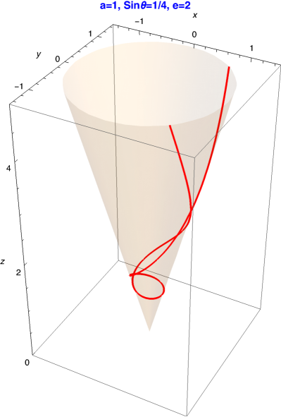
Figure 1: A conic-shaped orbit of the binary that is confined to the surface of a cone by choosing the parameters $a=1$, $e=2$, and $\sin\theta=1/4$.

II.2 Gravitational and electromagnetic radiation from BBHs with electric and magnetic charges

In this subsection, we will focus on gravitational and electromagnetic radiation. Let us start by considering gravitational radiation. According to Ref. Peters and Mathews (1963), the radiated power of GWs due to gravitational quadrupole radiation, $\frac{dE_{\mathrm{GW}}^{\mathrm{quad}}}{dt}$, is expressed as

$$\frac{dE_{\mathrm{GW}}^{\mathrm{quad}}}{dt}=-\frac{1}{5}\left(\dddot{Q}_{ij}\dddot{Q}_{ij}\right)=-\frac{1}{5}\left(\dddot{M}_{ij}\dddot{M}_{ij}-\frac{1}{3}\left(\dddot{M}_{kk}\right)^{2}\right),$$ (9)

where $M_{ij}$ is the second mass moment, and $Q_{ij}\equiv M_{ij}-\frac{1}{3}\delta_{ij}M_{kk}$ is traceless second mass moment. In our reference frame where $\bm{L}$ is along $z$ axis, the second mass moment $M_{ij}$ takes the $3\times 3$ matrix form as

$$M^{ij}=\mu R_{i}R_{j}=\mu R^{2}\left(\begin{array}[]{ccc}\sin^{2}\theta\cos^{2}\phi&\sin^{2}\theta\cos\phi\sin\phi&\sin\theta\cos\theta\cos\phi\\ \sin^{2}\theta\cos\phi\sin\phi&\sin^{2}\theta\sin^{2}\phi&\sin\theta\cos\theta\sin\phi\\ \sin\theta\cos\theta\cos\phi&\sin\theta\cos\theta\sin\phi&\cos^{2}\theta\end{array}\right).$$ (10)

From Eq. (9), to obtain the radiated power of GWs, we need to compute the third derivative of $M_{ij}$. Notice that the components $M_{ij}$ depend on $\psi$, so one way to compute their derivatives is using $\dot{\phi}$ that is given by

$$\dot{\phi}=\frac{\tilde{L}}{\mu R^{2}\sin\theta}=\frac{\sqrt{\text{-C}}\csc\theta(e\cos(\phi\sin\theta)-1)^{2}}{a^{3/2}\left(e^{2}-1\right)^{3/2}\sqrt{\mu}}.$$ (11)

Then, using the chain rule, $\dot{M}_{ij}$ in terms of $\dot{\phi}$ is given by $\dot{M}_{ij}=\frac{dM_{ij}}{d\phi}\dot{\phi}$. Moreover, we can extend the same idea to the second and third derivatives. Therefore, we could arrive at

$$\dddot{M}_{ij}=\frac{\left(-C\right)^{3/2}\beta_{ij}}{a^{5/2}\left(e^{2}-1\right)^{5/2}\sqrt{\mu}},$$ (12)

where $\beta_{ij}$ is a function of $e$, $\theta$, and $\phi$. The components of $\beta_{ij}$ are given by

$$\beta_{11}= 2\csc\theta\cos\phi(e\cos(\phi\sin\theta)-1)^{2}$$ (13)

$$\times\left[4\sin\phi(e\cos(\phi\sin\theta)-1)\left(e\cos^{2}\theta\cos(\phi\sin\theta)-1\right)+e\sin^{3}\theta\cos\phi\sin(\phi\sin\theta)\right],$$

$$\beta_{12}= \beta_{21}=2\csc\theta(e\cos(\phi\sin\theta)-1)^{2}\Bigl{[}2\sin^{2}\phi(e\cos(\phi\sin\theta)-1)\left(e\cos^{2}\theta\cos(\phi\sin\theta)-1\right)$$

$$-2\cos^{2}\phi(e\cos(\phi\sin\theta)-1)\left(e\cos^{2}\theta\cos(\phi\sin\theta)-1\right)+e\sin^{3}\theta\sin\phi\cos\phi\sin(\phi\sin\theta)\Bigr{]},$$

$$\beta_{13}= \beta_{31}=\cot\theta\csc\theta(e\cos(\phi\sin\theta)-1)^{2}$$

$$\times\left[2e\sin^{3}\theta\cos\phi\sin(\phi\sin\theta)+\sin\phi(e\cos(\phi\sin\theta)-1)(e(2\cos(2\theta)-1)\cos(\phi\sin\theta)-1)\right],$$

$$\beta_{22}= 2\csc\theta\sin\phi(e\cos(\phi\sin\theta)-1)^{2}$$

$$\times\left[e\sin^{3}\theta\sin\phi\sin(\phi\sin\theta)-4\cos\phi(e\cos(\phi\sin\theta)-1)\left(e\cos^{2}\theta\cos(\phi\sin\theta)-1\right)\right],$$

$$\beta_{23}= \beta_{32}=\cot\theta\csc\theta(e\cos(\phi\sin\theta)-1)^{2}$$

$$\times\left[2e\sin^{3}\theta\sin\phi\sin(\phi\sin\theta)+\cos\phi(e\cos(\phi\sin\theta)-1)((e-2e\cos(2\theta))\cos(\phi\sin\theta)+1)\right],$$

$$\beta_{33}= 2e\cos^{2}\theta\sin(\phi\sin\theta)(e\cos(\phi\sin\theta)-1)^{2}.$$

Using Eq. (9), we can obtain the radiated power of GWs, $\frac{dE_{\mathrm{GW}}^{\mathrm{quad}}}{dt}$, and the total energy loss due to gravitational quadrupole radiation, $\Delta E_{\mathrm{GW}}$,

$$\frac{dE_{\mathrm{GW}}^{\mathrm{quad}}}{dt}=\frac{C^{3}}{a^{5}\left(e^{2}-1\right)^{5}\mu}\mathcal{G}_{1}(\theta,\phi,e),$$ (14)

$$\Delta E_{\mathrm{GW}}^{\mathrm{quad}}=\int^{\infty}_{-\infty}\frac{dE_{\mathrm{GW}}^{\mathrm{quad}}}{dt}dt=\int^{2\pi/\sin\theta-\phi_{1}}_{\phi_{1}}\frac{dE_{\mathrm{GW}}^{\mathrm{quad}}}{dt}(\frac{d\phi}{dt})^{-1}d\phi=-\frac{(-C)^{5/2}}{a^{7/2}\left(e^{2}-1\right)^{7/2}\sqrt{\mu}}\mathcal{G}_{2}(\theta,e),$$ (15)

where

$$\mathcal{G}_{1} =\frac{\csc^{4}\theta}{120}(e\cos(\phi\sin\theta)-1)^{4}\Bigl{\{}9e^{4}\cos(4\phi\sin\theta)+12e\Bigl{[}e\left(\left(3e^{2}+35\right)\cos(2\phi\sin\theta)-7e\cos(3\phi\sin\theta)\right)$$ (16)

$$-21\left(e^{2}+4\right)\cos(\phi\sin\theta)\Bigr{]}-2e\cos(4\theta)\Bigl{[}e(3e^{2}\cos(4\phi\sin\theta)+2\left(6e^{2}+43\right)\cos(2\phi\sin\theta)$$

$$+9e^{2}-30e\cos(3\phi\sin\theta)+82)-18\left(5e^{2}+4\right)\cos(\phi\sin\theta)\Bigr{]}+\cos(2\theta)\Bigl{[}3e^{4}\cos(4\phi\sin\theta)$$

$$+4e\left(6\left(28-3e^{2}\right)\cos(\phi\sin\theta)+\left(3e^{3}-26e\right)\cos(2\phi\sin\theta)-6e^{2}\cos(3\phi\sin\theta)\right)$$

$$+9e^{4}-136e^{2}-360\Bigr{]}+27e^{4}+444e^{2}+408\Bigr{\}},$$

$$\mathcal{G}_{2} =\frac{\csc^{4}\theta}{1800}\Bigl{\{}-15\arccos(e^{-1})\Bigl{[}2\left(15e^{4}+323e^{2}+308\right)e^{2}\cos(4\theta)+\left(-15e^{6}+26e^{4}+1976e^{2}+720\right)$$ (17)

$$\times\cos(2\theta)-3\left(15e^{6}+404e^{4}+1104e^{2}+272\right)\Bigr{]}+450\pi e^{6}\cos(4\theta)+4926\sqrt{e^{2}-1}e^{4}\cos(4\theta)$$

$$+9690\pi e^{4}\cos(4\theta)+13658\sqrt{e^{2}-1}e^{2}\cos(4\theta)+9240\pi e^{2}\cos(4\theta)+796\sqrt{e^{2}-1}\cos(4\theta)$$

$$+(-225\pi e^{6}-2079\sqrt{e^{2}-1}e^{4}+390\pi e^{4}+20368\sqrt{e^{2}-1}e^{2}+29640\pi e^{2}+22316\sqrt{e^{2}-1}$$

$$+10800\pi)\cos(2\theta)-675\pi e^{6}-7005\sqrt{e^{2}-1}e^{4}-18180\pi e^{4}-47130\sqrt{e^{2}-1}e^{2}$$

$$-49680\pi e^{2}-26640\sqrt{e^{2}-1}-12240\pi\Bigr{\}}.$$

Now, let us calculate the emission of electromagnetic dipole and quadrupole radiation due to the electric and magnetic charges on the orbit (7). According to Ref. Liu et al. (2020a) and Appendix A, the energy emission rate due to electromagnetic dipole radiation $P_{\mathrm{EM}}$ is

$$\frac{dE_{\mathrm{EM}}^{\mathrm{dip}}}{dt}=-\frac{2\mu^{2}((\Delta\sigma_{q})^{2}+(\Delta\sigma_{g})^{2})}{3}\ddot{R}^{i}\ddot{R}_{i},$$ (18)

where $\Delta\sigma_{q}=q_{2}/m_{2}-q_{1}/m_{1}$ and $\Delta\sigma_{g}=g_{2}/m_{2}-g_{1}/m_{1}$ are the dipole moments of electric charges and magnetic charges. Hence, the radiated power of electromagnetic waves, $\frac{dE_{\mathrm{EM}}^{\mathrm{dip}}}{dt}$, and the total energy loss due to electromagnetic radiation, $\Delta E_{\mathrm{GW}}$, are given by

$$\frac{dE_{\mathrm{EM}}^{\mathrm{dip}}}{dt}=-\frac{((\Delta\sigma_{q})^{2}+(\Delta\sigma_{g})^{2})C^{2}}{a^{4}\left(e^{2}-1\right)^{4}}\mathcal{K}_{1}(\theta,\phi,e)$$ (19)

$$\Delta E_{\mathrm{EM}}^{\mathrm{dip}}=\int^{\infty}_{-\infty}\frac{dE_{\mathrm{EM}}^{\mathrm{dip}}}{dt}dt=\int^{2\pi/\sin\theta-\phi_{1}}_{\phi_{1}}\frac{dE_{\mathrm{EM}}^{\mathrm{dip}}}{dt}(\frac{d\phi}{dt})^{-1}d\phi=-\frac{((\Delta\sigma_{q})^{2}+(\Delta\sigma_{g})^{2})(-C)^{3/2}\sqrt{\mu}}{a^{5/2}\left(e^{2}-1\right)^{5/2}}\mathcal{K}_{2}(\theta,e),$$ (20)

where

$$\mathcal{K}_{1} =\frac{\csc^{2}\theta}{12}(e\cos(\phi\sin\theta)-1)^{4}\Bigl{(}2e^{2}\cos(2\phi\sin\theta)+e^{2}\cos(2\phi\sin\theta+2\theta))+e^{2}\cos(2\theta-2\phi\sin\theta)$$ (21)

$$+2e^{2}\cos(2\theta)+2e^{2}-8e\cos(\phi\sin\theta)-4e\cos(\phi\sin\theta+2\theta)-4e\cos(2\theta-\phi\sin\theta)+8\Bigr{)},$$

$$\mathcal{K}_{2} =\frac{\csc^{2}\theta}{36}\Bigl{(}-3\arccos(e^{-1})\left(\left(3e^{2}+20\right)e^{2}\cos(2\theta)+3e^{4}+28e^{2}+16\right)+(9\pi e^{4}+55\sqrt{e^{2}-1}e^{2}$$ (22)

$$+60\pi e^{2}+14\sqrt{e^{2}-1})\cos(2\theta)+9\pi e^{4}+55\sqrt{e^{2}-1}e^{2}+84\pi e^{2}+86\sqrt{e^{2}-1}+48\pi\Bigr{)}.$$

From Appendix A, the relation between electromagnetic quadrupole radiation and gravitational quadrupole radiation is given by

$$\frac{dE_{\mathrm{EM}}^{\mathrm{quad}}}{dt}\equiv\frac{\mu^{2}((q_{2}/m_{2}^{2}+q_{1}/m_{1}^{2})^{2}+(g_{2}/m_{2}^{2}+g_{1}/m_{1}^{2})^{2})}{4}\frac{dE_{\mathrm{GW}}^{\mathrm{quad}}}{dt}.$$ (23)

Furthermore, the contribution of the quadrupole term of electromagnetic radiation is always smaller than the quadrupole term of gravitational radiation. Therefore, the total energy loss due to electromagnetic dipole and quadrupole radiation and gravitational quadrupole radiation is given by

$$\Delta E=\Delta E_{\mathrm{EM}}^{\mathrm{dip}}+\Delta E_{\mathrm{EM}}^{\mathrm{quad}}+\Delta E_{\mathrm{GW}}^{\mathrm{quad}}=\Delta E_{\mathrm{EM}}^{\mathrm{dip}}+\left(1+\Lambda\right)\Delta E_{\mathrm{GW}}^{\mathrm{quad}},$$ (24)

where $\Lambda=\frac{\mu^{2}((q_{2}/m_{2}^{2}+q_{1}/m_{1}^{2})^{2}+(g_{2}/m_{2}^{2}+g_{1}/m_{1}^{2})^{2})}{4}$. In this Section, we have calculated the total emission rates of energy due to gravitational and electromagnetic radiation from BBHs with electric and magnetic charges in hyperbolic orbits. In the universe, the two-body dynamical capture is an absolutely common and effective way to form BBH systems. We will derive the merger rate of BBHs with electric and magnetic charges from the two-body dynamical capture in the next Section.

III Merger rate of BBHs with electric and magnetic charges from the two-body dynamical capture

If two BHs with electric and magnetic charges are getting closer and closer, the total energy loss due to gravitational and electromagnetic radiation could exceed the orbital kinetic energy. Hence the unbound system cannot escape to infinity anymore and will form a bound binary with negative orbital energy. Therefore, this binary immediately merges through consequent large electromagnetic and gravitational radiation. For such a process, we can estimate the cross section and calculate the merger rate of BBHs with electric and magnetic charges from the two-body dynamical capture.

Let us consider the interaction of two dyonic BHs with masses and charges ($m_{1}$, $q_{1}$, $g_{1}$) and ($m_{2}$, $q_{2}$, $g_{2}$), and assume that they have an initial relative velocity $v$, the impact parameter $b$ and the distance of periastron $r_{p}$. According to the definition of $r_{p}$ and the orbit (7), we have $r_{p}\equiv R_{min}=R(\phi=\frac{\pi}{\sin\theta})=a(e-1)$. We could approximate the trajectory of a close encounter by the hyperbolic with $e\rightarrow 1$ since when the two dyonic BHs pass by closer and closer, the true trajectory is physically indistinguishable from a parabolic one near the periastron where electromagnetic and gravitational radiation dominantly occurs. According to Sec. II, the total energy loss due to electromagnetic radiation and gravitational radiation by the close encounter can be evaluated by using $e\rightarrow 1$ and the periastron $r_{p}\equiv a(e-1)$, namely

$$\Delta E_{\mathrm{EM}}^{\mathrm{dip}}+\left(1+\Lambda\right)\Delta E_{\mathrm{GW}}^{\mathrm{quad}}$$ (25)

where

$$\Delta E_{\mathrm{EM}}^{\mathrm{dip}}=-\frac{\pi((\Delta\sigma_{q})^{2}+(\Delta\sigma_{g})^{2})(-C)^{3/2}\sqrt{\mu}(23\cos(2\theta)+47)\csc^{2}(\theta)}{48\sqrt{2}r_{p}^{5/2}},$$ (26)

$$\Delta E_{\mathrm{{GW}}}^{\mathrm{quad}}=-\frac{\pi(-C)^{5/2}(-2707\cos(2\theta)-1292\cos(4\theta)+5385)\csc^{4}\theta}{960\sqrt{2}\sqrt{\mu}r_{p}^{7/2}}.$$ (27)

The definition of the impact parameter $b$ is the distance from the origin to the asymptotes of the hyperbolic orbit. One asymptote of the hyperbolic orbit is given by

$$x =\lim_{\phi\rightarrow\phi_{1}}\left(\frac{a\left(e^{2}-1\right)}{1-e\cos(\phi\sin\theta)}\sin\theta\cos\phi\right)-l\sin\theta\cos\phi_{1},$$ (28)

$$y =\lim_{\phi\rightarrow\phi_{1}}\left(\frac{a\left(e^{2}-1\right)}{1-e\cos(\phi\sin\theta)}\sin\theta\sin\phi\right)-l\sin\theta\sin\phi_{1},$$

$$z =\lim_{\phi\rightarrow\phi_{1}}\left(\frac{a\left(e^{2}-1\right)}{1-e\cos(\phi\sin\theta)}\cos\theta\right)-l\cos\theta.$$

Here, when choosing $y_{0}=0$, we can get the solution of $l_{0}$,

$$l=\lim_{\phi\rightarrow\phi_{1}}\left(\frac{a\left(e^{2}-1\right)}{1-e\cos(\phi\sin\theta)}\frac{\sin\phi}{\sin\phi_{1}}\right).$$ (29)

From Eqs. (28) and (29), when $y_{0}=0$, $x_{0}$ and $z_{0}$ are expressed as

$$x_{0} =\lim_{\phi\rightarrow\phi_{1}}\left(\frac{a\left(e^{2}-1\right)}{1-e\cos(\phi\sin\theta)}\sin\theta\cos\phi-\frac{a\left(e^{2}-1\right)}{1-e\cos(\phi\sin\theta)}\frac{\sin\phi}{\sin\phi_{1}}\sin\theta\cos\phi_{1}\right)$$ (30)

$$=-a\sqrt{e^{2}-1}\csc\left(\arccos(e^{-1})\csc\theta\right),$$

$$z_{0} =\lim_{\phi\rightarrow\phi_{1}}\left(\frac{a\left(e^{2}-1\right)}{1-e\cos(\phi\sin\theta)}\cos\theta-\frac{a\left(e^{2}-1\right)}{1-e\cos(\phi\sin\theta)}\frac{\sin\phi}{\sin\phi_{1}}\cos\theta\right)$$

$$=-a\sqrt{e^{2}-1}\cot\theta\cot\left(\arccos(e^{-1})\csc\theta\right).$$

Therefore, we get the point of intersection of the asymptotes and $x$-$z$ plane, $(x_{0},0,z_{0})$. We denote the vector $\vec{v_{1}}$ as $\vec{v}_{1}=(x_{0},0,z_{0})$. Using the unit vector along the asymptotes of the hyperbolic orbit, $\vec{v}_{2}=\left(\sin\theta\cos\phi_{1},\sin\theta\sin\phi_{1},\cos\theta\right)$, the impact parameter $b$ is given by

$$b=\sqrt{\vec{v}_{1}\cdot\vec{v}_{1}-(\vec{v}_{1}\cdot\vec{v}_{2})^{2}}=a\sqrt{e^{2}-1},$$ (31)

which is independent of $\theta$. It shows that no matter the orbit is three-dimensional ($\theta\neq\pi/2$) or two-dimensional ($\theta=\pi/2$), we always have $b=a\sqrt{e^{2}-1}$. From Eq. (31) and $r_{p}\equiv a(e-1)$, we can get $b^{2}=r_{p}^{2}+2ar_{p}$. Note that the total energy can be expressed as $E\equiv-\frac{C}{2a}=\frac{\mu v^{2}}{2}$, so $a=-\frac{C}{\mu v^{2}}$. Therefore, we find the relation between $r_{p}$ and $b$ as

$$b^{2}=r_{p}^{2}-\frac{2Cr_{p}}{\mu v^{2}}.$$ (32)

In the limit of a strong electromagnetic and gravitational radiation focusing, i.e. $r_{p}\ll b$, then we get the distance of the closest approach $r_{p}$ as

$$r_{p}=-\frac{\mu v^{2}b^{2}}{2C}.$$ (33)

The condition for the dyonic BHs to form a bound system is that the total energy loss due to electromagnetic and gravitational radiation is larger than the kinetic energy $\mu v^{2}/2$, i.e.,

$$\Delta E+\frac{\mu v^{2}}{2}<0.$$ (34)

From Eqs. (33) and (34), we could obtain the merging cross-section $\sigma=\pi b_{\max}^{2}$, where $b_{\max}$ is the maximum impact parameter for the dyonic BHs to form a bound system and is determined by

$$\frac{\pi(\Lambda+1)C^{6}(5385-2707\cos(2\theta)-1292\cos(4\theta))\csc^{4}\theta}{120b_{\max}^{7}\mu^{4}v^{7}}$$ (35)

$$+ \frac{\pi((\Delta\sigma_{q})^{2}+(\Delta\sigma_{g})^{2})C^{4}(23\cos(2\theta)+47)\csc^{2}\theta}{12b_{\max}^{5}\mu^{2}v^{5}}=\frac{\mu v^{2}}{2}.$$

Here, we want to reminder the reader that $\theta$ is a function of $b_{\max}$ and is given by $\cos^{2}\theta=\frac{D^{2}}{D^{2}+\mu^{2}v^{2}b_{\max}^{2}}$. Finally, we could achieve the differential merger rate of dyonic BHs from the two-body dynamical capture,

$$dR=n(m_{1},q_{1},g_{1})n(m_{2},q_{2},g_{2})\left\langle\sigma v\right\rangle dm_{1}dm_{2}dq_{1}dq_{2}dg_{1}dg_{2}$$ (36)

where $\left\langle\sigma v\right\rangle$ denotes the average over relative velocity distribution with $\sigma=\pi b_{\max}^{2}$ in Eq. (31) and $n(m_{1},q_{1},g_{1})$ and $n(m_{2},q_{2},g_{2})$ are the comoving average number density of dyonic BHs with mass, electric and magnetic charges ($m_{1}$, $q_{1}$, $g_{1}$) and ($m_{2}$, $q_{2}$, $g_{2}$). In this section, we develop a formalism to derive the merger rate of BBHs with electric and magnetic charges from the two-body dynamical capture. Next, we will apply the formalism to find the effects of the charges on the merger rate for the near-extremal case.

IV Effects of the charges on the merger rate for the near-extremal case

The origin of those BHs with electric and magnetic charges may be the primordial BH (PBH) which are BHs formed in the radiation-dominated era of the early Universe due to the collapse of large energy density fluctuations Zel’dovich (1967); Hawking (1971); Carr and Hawking (1974). A PBH can be magnetized by the accretion of monopoles in the early Universe. For instance, PBHs in a strong magnetic field can produce a pair of magnetic monopoles through pair production Das and Hook (2021); Kobayashi (2021). The magnetized PBH can also produce a strong magnetic field, which results in the accretion of electric charges Wald (1974). This is the mechanism for BHs to have electric and magnetic charges in the early Universe. Recently, Ref. Kritos and Silk (2022) shows that PBHs can be near-extremal charged. In this section, we will apply the formalism developed in the last section to find the effects of the charges on the merger rate for the near-extremal case. For simplicity, we consider a special model assuming that all PBHs have the same mass $M_{\mathrm{PBH}}$. In such a model, the number density of dyonic PBHs is given by

$$n(m,q,g)=\frac{1}{4}\frac{f_{\mathrm{PBH}}\rho_{\mathrm{DM}}}{M_{\mathrm{PBH}}}\left(\delta(\frac{q}{m}-\iota_{e})+\delta(\frac{q}{m}+\iota_{e})\right)\left(\delta(\frac{g}{m}-\iota_{m})+\delta(\frac{g}{m}+\iota_{m})\right)\delta(m-M_{\mathrm{PBH}}),$$ (37)

where $\rho_{\mathrm{DM}}$ is the dark matter energy density at present, and $f_{\mathrm{PBH}}$ is the fraction of PBHs in the dark matter. This model suggests that the part of the Universe under study is charge neutral, but charges are locally separated by some mechanisms found in Refs. Wald (1974); Bai and Orlofsky (2020). Here, we only consider the near-extremal case. In other words, we take $\iota_{m}\equiv\sqrt{1-\iota_{e}^{2}}$. For simplicity, we choose $\iota_{e}\geq 0$. In the calculation, we take the Maxwell-Boltzmann distribution $P(v)\propto v^{2}\exp\left(-v^{2}/v_{0}^{2}\right)$ for the velocity distribution of BHs with the most probable velocity $v_{0}=100$ km/s. For the charge-neutral Schwarzschild BHs, the merger rate of PBH binaries from the two-body capture is $R_{\mathrm{Sch}}\approx 1.5\times 10^{-8}f_{\mathrm{PBH}}^{2}\mathrm{Gpc}^{-3}\mathrm{yr}^{-1}$ that is independent of $M_{\mathrm{PBH}}$ and scales as $f_{\mathrm{PBH}}^{2}$.

To show the effects of charges $\iota_{e}$ on the merger rate of PBH binaries from the two-body dynamical capture for the near-extremal case, we define a function of $\iota_{e}$ as

$$\eta(\iota_{e})\equiv\frac{R(\iota_{e})}{R_{\mathrm{Sch}}},$$ (38)

where $R(\iota_{e})$ is the total merger rate of near-extremal PBH binaries with electric charge-to-mass ratio $\iota_{e}$ and $R_{\mathrm{Sch}}$ is the total merger rate of PBH binaries in charge-neutral case. In this special model, $C$ equals to $-M_{\mathrm{PBH}}^{2}\left(1\pm\iota_{e}^{2}\pm\left(1-\iota_{e}^{2}\right)\right)$, and $D$ equals to $0,\pm 2\iota_{e}\sqrt{1-\iota_{e}^{2}}M_{\mathrm{PBH}}^{2}$ in different cases as shown in Table 1. The total merger rate of near-extremal PBH binaries, $R(\iota_{e})$, is the sum of the merger rate of different cases. Notice that from Eq. (LABEL:bb) it follows $b_{\max}\propto M_{\mathrm{PBH}}$ and $\sigma\propto M_{\mathrm{PBH}}^{2}$, we find that $R(\iota_{e})$ is independent of $M_{\mathrm{PBH}}$ and scales as $f_{\mathrm{PBH}}^{2}$. Therefore, $\eta(\iota_{e})$ is independent of $M_{\mathrm{PBH}}$ and $f_{\mathrm{PBH}}$ and is only a function of $\iota_{e}$. In Fig. 2, we plot $\eta(\iota_{e})$ as the function of $\iota_{e}$. From the definition, we find $\eta(\iota_{e})=\eta(\sqrt{1-\iota_{e}^{2}})$ and show that $\eta(\iota_{e})$ decreases as $\iota_{e}$ increases and reaches the minimum value of $\eta(\frac{\sqrt{2}}{2})\approx 6.3$ in $\iota_{e}\in[0,\frac{\sqrt{2}}{2}]$. For $\iota_{e}\in[\frac{\sqrt{2}}{2},1]$, $\eta(\iota_{e})$ increases as $\iota_{e}$ increases and reaches the maximum value of $\eta(1)\approx 8.4$. As shown in Fig. 2, the effects of the charges on the merger rate for the near-extremal case cannot be ignored. In Fig. 2, we also show that the averaged merging cross section is always much larger than that corresponding to the event horizon radius. Therefore, the Newtonian approximation is sufficiently accurate.

	$q_{1}=q_{2}\geq 0$	$q_{1}=-q_{2}\geq 0$	$q_{1}=q_{2}<0$	$q_{1}=-q_{2}<0$
$g_{1}=g_{2}\geq 0$	$C=0$	$C=-2\iota_{e}^{2}M_{\mathrm{PBH}}^{2}$	$C=0$	$C=2\iota_{e}^{2}M_{\mathrm{PBH}}^{2}$
	$D=0$	$D=-2\iota_{e}\iota_{m}M_{\mathrm{PBH}}^{2}$	$D=0$	$D=-2\iota_{e}\iota_{m}M_{\mathrm{PBH}}^{2}$
$g_{1}=-g_{2}\geq 0$	$C=-2\iota_{m}^{2}M_{\mathrm{PBH}}^{2}$	$C=-2M_{\mathrm{PBH}}^{2}$	$C=-2\iota_{m}^{2}M_{\mathrm{PBH}}^{2}$	$C=-2M_{\mathrm{PBH}}^{2}$
	$D=2\iota_{e}\iota_{m}M_{\mathrm{PBH}}^{2}$	$D=0$	$D=-2\iota_{e}\iota_{m}M_{\mathrm{PBH}}^{2}$	$D=0$
$g_{1}=g_{2}<0$	$C=0$	$C=-2\iota_{e}^{2}M_{\mathrm{PBH}}^{2}$	$C=0$	$C=-2\iota_{e}^{2}M_{\mathrm{PBH}}^{2}$
	$D=0$	$D=2\iota_{e}\iota_{m}M_{\mathrm{PBH}}^{2}$	$D=0$	$D=-2\iota_{e}\iota_{m}M_{\mathrm{PBH}}^{2}$
$g_{1}=-g_{2}<0$	$C=-2\iota_{m}^{2}M_{\mathrm{PBH}}^{2}$	$C=-2M_{\mathrm{PBH}}^{2}$	$C=-2\iota_{m}^{2}M_{\mathrm{PBH}}^{2}$	$C=-2M_{\mathrm{PBH}}^{2}$
	$D=-2\iota_{e}\iota_{m}M_{\mathrm{PBH}}^{2}$	$D=0$	$D=2\iota_{e}\iota_{m}M_{\mathrm{PBH}}^{2}$	$D=0$

Table 1: The value of $C$ and $D$ in different cases.

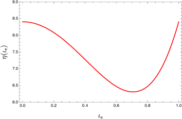
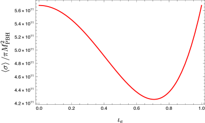
Figure 2: Left: The plot of $\eta(\iota_{e})$ as a function of $\iota_{e}$. Right: The plot of $\left\langle\sigma\right\rangle/\pi M_{\mathrm{PBH}}^{2}$ as a function of $\iota_{e}$.

V Conclusion

In this work, we have derived the hyperbolic orbit of BBHs with electric and magnetic charges. In the low-velocity and weak-field regime, by using a Newtonian method, we calculate the total emission rate of energy due to gravitational and electromagnetic radiation from BBHs with electric and magnetic charges in hyperbolic orbits. We also develop a formalism to derive the merger rate of BBHs with electric and magnetic charges from the two-body dynamical capture. We apply this formalism to estimate the effects of the charges on the merger rate for the near-extremal case and find that the effects cannot be ignored.

In our calculation, we don’t assume the mass of binary. For the solar mass range, combined with Ref. Liu et al. (2020a, 2021), the results of this work could provide rich information and a crosscheck to test whether LIGO-Virgo-KAGRA black holes have electric and magnetic charges. On the other hand, those BBHs whose mass is smaller than one solar masses must be PBHs instead of astrophysical BHs. Those extremal charged PBHs are stable and could account for all dark matter without requiring physics beyond the standard model, even though there are many constraints for uncharged PBHs as dark matter Sasaki et al. (2018); Carr et al. (2021); Carr and Kuhnel (2020). Two extremal-charged PBHs with opposite charges could form a bound system through the two-body capture. When they merge, the burst of gamma rays due to the annihilation of charges could be detected by observations.

We find that the BHs with electric and magnetic charges can form a bound system due to gravitational and electromagnetic radiation. Another possibility is that charged BHs do not end up with a bound system in a single encounter but inspiral and enter another scattering event through a hyperbolic encounter. For two BHs with electric and magnetic charges, if the relative velocity or distance is large enough, then the two-body capture cannot happen. These events, however, can generate bursts of GWs. Compared with the GW burst produced by the encounter of Schwarzschild BHs, the GW burst produced by the encounter of BHs with electric and magnetic charges has different characteristics and phenomena. The characteristic peak frequency and detection of such GW bursts is an interesting issue, and we will leave this topic for future work.

Appendix A Electromagnetic dipole and quadrupole radiation from dyonic BBHs

When the differences $\Delta\sigma_{q}$ of electric charge-to-mass ratios and $\Delta\sigma_{g}$ of magnetic charge-to-mass ratios are very small or even vanishes, the charge quadrupole might be extremely important. Here, we will consider the electromagnetic dipole and quadrupole radiation from dyonic BBHs. We first derive the emission of electromagnetic radiation from electric charges, then calculate the emission from magnetic charges, and finally superimpose their fields.

Following Ref. Liu and Kim (2022b), the energy emission due to electromagnetic dipole and quadrupole radiation is given by

$$\frac{dE_{\mathrm{EM}}}{dt}|_{e}=\frac{dE_{\mathrm{EM}}^{\mathrm{dip}}}{dt}|_{e}+\frac{dE_{\mathrm{EM}}^{\mathrm{quad}}}{dt}|_{e},$$ (39)

and

$$\frac{dE_{\mathrm{EM}}^{\mathrm{dip}}}{dt}|_{e}=-\frac{2\ddot{p}^{2}}{3},$$ (40)

$$\frac{dE_{\mathrm{EM}}^{\mathrm{quad}}}{dt}|_{e}=-\frac{\ddddot{D}_{ij}\ddddot{D}_{ij}}{20}.$$ (41)

where $p^{i}=\mu\Delta\sigma_{q}R^{i}$ is electric charge dipole and $D^{ij}=\mu\left(\frac{Q_{1}}{m_{1}^{2}}+\frac{Q_{2}}{m_{2}^{2}}\right)Q^{ij}$ is traceless electric charge quadrupole.

An important consequence of the enhanced symmetry due to the existence of magnetic monopoles is that the classical dynamics of the charges, fields and Maxwell’s equations are all invariant under the dual transformation,

$$\begin{aligned} &\bm{E}^{\prime}=\bm{E}\cos\alpha-\bm{B}\sin\alpha,\\ &\bm{B}^{\prime}=\bm{E}\sin\alpha+\bm{B}\cos\alpha,\\ &q^{\prime}=q\cos\alpha+g\sin\alpha,\\ &g^{\prime}=g\cos\alpha-g\sin\alpha.\end{aligned}$$ (42)

Choosing $\alpha=\pi/2$, pure electric charges could transform to pure magnetic charges. This helps us to directly find the fields emanating from magnetic charges from the results for pure electric charges. For $\alpha=\pi/2$, it is easy to find $\bm{E}_{2}\propto\bm{B}_{1}$ and $\bm{B}_{2}\propto\bm{E}_{1}$ by labeling the fields from the electric charge, $\bm{E}_{1},\bm{B}_{1},$ and those from the dual transformation, $\bm{E}_{2},\bm{B}_{2}$. Now, we consider the integrated energy density on a shell for electric and magnetic fields. Notice that the electric dipole and quadruple have the same direction as the magnetic dipole and quadruple. Therefore, we get $\bm{E}_{1}\perp\bm{E}_{2}$, $\bm{B}_{1}\perp\bm{B}_{2}$, $\bm{E}_{1}||\bm{B}_{2}$, and $\bm{E}_{2}||\bm{B}_{1}$. We then consider the result for the energy density and momentum density

$$u=\frac{1}{2}\left(E^{2}+B^{2}\right)=\frac{1}{2}(E_{1}^{2}+B_{1}^{2}+E_{2}^{2}+B_{2}^{2}+2\left(\bm{E}_{1}\cdot\bm{E}_{2}+\bm{B}_{1}\cdot\bm{B}_{2}\right))=u_{1}+u_{2},$$ (43)

$$\bm{\mathcal{P}}=\bm{E}\times\bm{B}=\bm{E}_{1}\times\bm{B}_{1}+\bm{E}_{2}\times\bm{B}_{2}+\bm{E}_{1}\times\bm{B}_{2}+\bm{E}_{2}\times\bm{B}_{1}=\bm{\mathcal{P}_{1}}+\bm{\mathcal{P}_{2}}.$$ (44)

Using $\frac{dE_{\mathrm{EM}}}{dt}=-r^{2}\int d\Omega\hat{r}\cdot\bm{\mathcal{P}}$, we get $\frac{dE_{\mathrm{EM}}}{dt}=\frac{dE_{\mathrm{EM}}}{dt}|_{e}+\frac{dE_{\mathrm{EM}}}{dt}|_{m}$. This means that the total energy emissions due to electromagnetic dipole and quadrupole radiation are given by

$$\frac{dE_{\mathrm{EM}}}{dt}=\frac{dE_{\mathrm{EM}}^{\mathrm{dip}}}{dt}+\frac{dE_{\mathrm{EM}}^{\mathrm{quad}}}{dt},$$ (45)

where

$$\frac{dE_{\mathrm{EM}}^{\mathrm{dip}}}{dt}=\frac{dE_{\mathrm{EM}}^{\mathrm{dip}}}{dt}|_{e}+\frac{dE_{\mathrm{EM}}^{\mathrm{dip}}}{dt}|_{m}=-\frac{2\mu^{2}((q_{2}/m_{2}-q_{1}/m_{1})^{2}+(g_{2}/m_{2}-g_{1}/m_{1})^{2})}{3}\ddot{R}^{i}\ddot{R}_{i},$$ (46)

$$\frac{dE_{\mathrm{EM}}^{\mathrm{quad}}}{dt}=\frac{dE_{\mathrm{EM}}^{\mathrm{quad}}}{dt}|_{e}+\frac{dE_{\mathrm{EM}}^{\mathrm{quad}}}{dt}|_{m}=-\frac{\mu^{2}((q_{2}/m_{2}^{2}+q_{1}/m_{1}^{2})^{2}+(g_{2}/m_{2}^{2}+g_{1}/m_{1}^{2})^{2})}{20}\dddot{Q}_{ij}\dddot{Q}_{ij}.$$ (47)

Notice that $\frac{dE_{\mathrm{GW}}^{\mathrm{quad}}}{dt}\equiv-\frac{1}{5}\left(\dddot{Q}_{ij}\dddot{Q}_{ij}\right)$, we obtain the relation between electromagnetic quadrupole radiation and gravitational quadrupole radiation,

$$\frac{dE_{\mathrm{EM}}^{\mathrm{quad}}}{dt}\equiv\frac{\mu^{2}((q_{2}/m_{2}^{2}+q_{1}/m_{1}^{2})^{2}+(g_{2}/m_{2}^{2}+g_{1}/m_{1}^{2})^{2})}{4}\frac{dE_{\mathrm{GW}}^{\mathrm{quad}}}{dt}.$$ (48)

From the metric constrains, $q_{1}^{2}+g_{1}^{2}\leq m_{1}^{2}$ and $q_{2}^{2}+g_{2}^{2}\leq m_{2}^{2}$, it is straightforward to prove that $\frac{dE_{\mathrm{EM}}^{i,\mathrm{quad}}}{dt}\leq\frac{1}{4}\frac{dE_{\mathrm{GW}}^{\mathrm{quad}}}{dt}$ is always hold.

References

- Abbott et al. (2016) B. P. Abbott et al. (LIGO Scientific, Virgo), “Observation of Gravitational Waves from a Binary Black Hole Merger,” Phys. Rev. Lett. 116, 061102 (2016), arXiv:1602.03837 [gr-qc] .
- Abbott et al. (2019a) B. P. Abbott et al. (LIGO Scientific, Virgo), “GWTC-1: A Gravitational-Wave Transient Catalog of Compact Binary Mergers Observed by LIGO and Virgo during the First and Second Observing Runs,” Phys. Rev. X9, 031040 (2019a), arXiv:1811.12907 [astro-ph.HE] .
- Abbott et al. (2021a) R. Abbott et al. (LIGO Scientific, Virgo), “GWTC-2: Compact Binary Coalescences Observed by LIGO and Virgo During the First Half of the Third Observing Run,” Phys. Rev. X 11, 021053 (2021a), arXiv:2010.14527 [gr-qc] .
- Abbott et al. (2021b) R. Abbott et al. (LIGO Scientific, VIRGO, KAGRA), “Gwtc-3: Compact binary coalescences observed by ligo and virgo during the second part of the third observing run,” (2021b), arXiv:2111.03606 [gr-qc] .
- Abbott et al. (2019b) B. P. Abbott et al. (LIGO Scientific, Virgo), “Tests of General Relativity with the Binary Black Hole Signals from the LIGO-Virgo Catalog GWTC-1,” Phys. Rev. D 100, 104036 (2019b), arXiv:1903.04467 [gr-qc] .
- Abbott et al. (2021c) R. Abbott et al. (LIGO Scientific, Virgo), “Tests of general relativity with binary black holes from the second LIGO-Virgo gravitational-wave transient catalog,” Phys. Rev. D 103, 122002 (2021c), arXiv:2010.14529 [gr-qc] .
- Abbott et al. (2021d) R. Abbott et al. (LIGO Scientific, VIRGO, KAGRA), “Tests of General Relativity with GWTC-3,” (2021d), arXiv:2112.06861 [gr-qc] .
- Staelens (2019) Michael Staelens (MoEDAL), “Recent Results and Future Plans of the MoEDAL Experiment,” in Meeting of the Division of Particles and Fields of the American Physical Society (2019) arXiv:1910.05772 [hep-ex] .
- Kobayashi (2021) Takeshi Kobayashi, “Monopole-antimonopole pair production in primordial magnetic fields,” Phys. Rev. D 104, 043501 (2021), arXiv:2105.12776 [hep-ph] .
- Maldacena (2021) Juan Maldacena, “Comments on magnetic black holes,” JHEP 04, 079 (2021), arXiv:2004.06084 [hep-th] .
- Bai et al. (2020) Yang Bai, Joshua Berger, Mrunal Korwar, and Nicholas Orlofsky, “Phenomenology of magnetic black holes with electroweak-symmetric coronas,” JHEP 10, 210 (2020), arXiv:2007.03703 [hep-ph] .
- Liu et al. (2020a) Lang Liu, Øyvind Christiansen, Zong-Kuan Guo, Rong-Gen Cai, and Sang Pyo Kim, “Gravitational and electromagnetic radiation from binary black holes with electric and magnetic charges: Circular orbits on a cone,” Phys. Rev. D 102, 103520 (2020a), arXiv:2008.02326 [gr-qc] .
- Ghosh et al. (2021) Diptimoy Ghosh, Arun Thalapillil, and Farman Ullah, “Astrophysical hints for magnetic black holes,” Phys. Rev. D 103, 023006 (2021), arXiv:2009.03363 [hep-ph] .
- Liu et al. (2021) Lang Liu, Øyvind Christiansen, Wen-Hong Ruan, Zong-Kuan Guo, Rong-Gen Cai, and Sang Pyo Kim, “Gravitational and electromagnetic radiation from binary black holes with electric and magnetic charges: elliptical orbits on a cone,” Eur. Phys. J. C 81, 1048 (2021), arXiv:2011.13586 [gr-qc] .
- Liu et al. (2020b) Lang Liu, Zong-Kuan Guo, Rong-Gen Cai, and Sang Pyo Kim, “Merger rate distribution of primordial black hole binaries with electric charges,” Phys. Rev. D 102, 043508 (2020b), arXiv:2001.02984 [astro-ph.CO] .
- Zilhao et al. (2012) Miguel Zilhao, Vitor Cardoso, Carlos Herdeiro, Luis Lehner, and Ulrich Sperhake, “Collisions of charged black holes,” Phys. Rev. D 85, 124062 (2012), arXiv:1205.1063 [gr-qc] .
- Zilhão et al. (2014) Miguel Zilhão, Vitor Cardoso, Carlos Herdeiro, Luis Lehner, and Ulrich Sperhake, “Collisions of oppositely charged black holes,” Phys. Rev. D 89, 044008 (2014), arXiv:1311.6483 [gr-qc] .
- Liebling and Palenzuela (2016) Steven L. Liebling and Carlos Palenzuela, “Electromagnetic Luminosity of the Coalescence of Charged Black Hole Binaries,” Phys. Rev. D94, 064046 (2016), arXiv:1607.02140 [gr-qc] .
- Toshmatov et al. (2018) Bobir Toshmatov, Zdeněk Stuchlík, Jan Schee, and Bobomurat Ahmedov, “Electromagnetic perturbations of black holes in general relativity coupled to nonlinear electrodynamics,” Phys. Rev. D 97, 084058 (2018), arXiv:1805.00240 [gr-qc] .
- Bai and Orlofsky (2020) Yang Bai and Nicholas Orlofsky, “Primordial Extremal Black Holes as Dark Matter,” Phys. Rev. D 101, 055006 (2020), arXiv:1906.04858 [hep-ph] .
- Allahyari et al. (2020) Alireza Allahyari, Mohsen Khodadi, Sunny Vagnozzi, and David F. Mota, “Magnetically charged black holes from non-linear electrodynamics and the Event Horizon Telescope,” JCAP 02, 003 (2020), arXiv:1912.08231 [gr-qc] .
- Christiansen et al. (2021) Øyvind Christiansen, Jose Beltrán Jiménez, and David F. Mota, “Charged Black Hole Mergers: Orbit Circularisation and Chirp Mass Bias,” Class. Quant. Grav. 38, 075017 (2021), arXiv:2003.11452 [gr-qc] .
- Wang et al. (2021) Hai-Tang Wang, Peng-Cheng Li, Jin-Liang Jiang, Guan-Wen Yuan, Yi-Ming Hu, and Yi-Zhong Fan, “Constrains on the electric charges of the binary black holes with GWTC-1 events,” The European Physical Journal C 81 (2021), 10.1140/epjc/s10052-021-09555-1.
- Bozzola and Paschalidis (2021a) Gabriele Bozzola and Vasileios Paschalidis, “General Relativistic Simulations of the Quasicircular Inspiral and Merger of Charged Black Holes: GW150914 and Fundamental Physics Implications,” Phys. Rev. Lett. 126, 041103 (2021a), arXiv:2006.15764 [gr-qc] .
- Kim and Kobakhidze (2020) Yunho Kim and Archil Kobakhidze, “Topologically induced black hole charge and its astrophysical manifestations,” (2020), arXiv:2008.04506 [gr-qc] .
- Cardoso et al. (2021a) Vitor Cardoso, Wen-Di Guo, Caio F. B. Macedo, and Paolo Pani, “The tune of the Universe: the role of plasma in tests of strong-field gravity,” Mon. Not. Roy. Astron. Soc. 503, 563–573 (2021a), arXiv:2009.07287 [gr-qc] .
- McInnes (2021a) Brett McInnes, “About Magnetic AdS Black Holes,” JHEP 03, 068 (2021a), arXiv:2011.07700 [gr-qc] .
- Bai and Korwar (2021) Yang Bai and Mrunal Korwar, “Hairy Magnetic and Dyonic Black Holes in the Standard Model,” JHEP 04, 119 (2021), arXiv:2012.15430 [hep-ph] .
- Diamond and Kaplan (2022) Melissa D. Diamond and David E. Kaplan, “Constraints on relic magnetic black holes,” JHEP 03, 157 (2022), arXiv:2103.01850 [hep-ph] .
- Bozzola and Paschalidis (2021b) Gabriele Bozzola and Vasileios Paschalidis, “Numerical-relativity simulations of the quasicircular inspiral and merger of nonspinning, charged black holes: Methods and comparison with approximate approaches,” Phys. Rev. D 104, 044004 (2021b), arXiv:2104.06978 [gr-qc] .
- McInnes (2021b) Brett McInnes, “The weak gravity conjecture requires the existence of exotic AdS black holes,” Nucl. Phys. B 971, 115525 (2021b), arXiv:2104.07373 [gr-qc] .
- Kritos and Silk (2022) Konstantinos Kritos and Joseph Silk, “Mergers of maximally charged primordial black holes,” Phys. Rev. D 105, 063011 (2022), arXiv:2109.09769 [gr-qc] .
- Hou et al. (2022) Shaoqi Hou, Shuxun Tian, Shuo Cao, and Zong-Hong Zhu, “Dark photon bursts from compact binary systems and constraints,” Phys. Rev. D 105, 064022 (2022), arXiv:2110.05084 [hep-ph] .
- Benavides-Gallego and Han (2021) Carlos A. Benavides-Gallego and Wen-Biao Han, “Phenomenological model for the electromagnetic response of a black hole binary immersed in magnetic field,” (2021), arXiv:2111.04323 [gr-qc] .
- Diamond et al. (2021) Melissa D. Diamond, David E. Kaplan, and Surjeet Rajendran, “Binary Collisions of Dark Matter Blobs,” (2021), arXiv:2112.09147 [hep-ph] .
- Ackerman et al. (2009) Lotty Ackerman, Matthew R. Buckley, Sean M. Carroll, and Marc Kamionkowski, “Dark Matter and Dark Radiation,” Phys. Rev. D 79, 023519 (2009), arXiv:0810.5126 [hep-ph] .
- Feng et al. (2009) Jonathan L. Feng, Manoj Kaplinghat, Huitzu Tu, and Hai-Bo Yu, “Hidden Charged Dark Matter,” JCAP 07, 004 (2009), arXiv:0905.3039 [hep-ph] .
- Foot and Vagnozzi (2015a) R. Foot and S. Vagnozzi, “Dissipative hidden sector dark matter,” Phys. Rev. D 91, 023512 (2015a), arXiv:1409.7174 [hep-ph] .
- Foot and Vagnozzi (2015b) R. Foot and S. Vagnozzi, “Diurnal modulation signal from dissipative hidden sector dark matter,” Phys. Lett. B 748, 61–66 (2015b), arXiv:1412.0762 [hep-ph] .
- Moffat (2006) J. W. Moffat, “Scalar-tensor-vector gravity theory,” JCAP 03, 004 (2006), arXiv:gr-qc/0506021 .
- Cardoso et al. (2016) Vitor Cardoso, Caio F. B. Macedo, Paolo Pani, and Valeria Ferrari, “Black holes and gravitational waves in models of minicharged dark matter,” JCAP 05, 054 (2016), [Erratum: JCAP 04, E01 (2020)], arXiv:1604.07845 [hep-ph] .
- Cardoso et al. (2021b) Vitor Cardoso, Caio F. B. Macedo, and Rodrigo Vicente, “Eccentricity evolution of compact binaries and applications to gravitational-wave physics,” Phys. Rev. D 103, 023015 (2021b), arXiv:2010.15151 [gr-qc] .
- Liu and Kim (2022a) Lang Liu and Sang Pyo Kim, “Gravitational and electromagnetic radiations from binary black holes with electric and magnetic charges,” in 17th Italian-Korean Symposium on Relativistic Astrophysics (2022) arXiv:2201.01138 [gr-qc] .
- Liu and Kim (2022b) Lang Liu and Sang Pyo Kim, “Merger rate of charged black holes from the two-body dynamical capture,” JCAP 03, 059 (2022b), arXiv:2201.02581 [gr-qc] .
- Zhang and Gong (2022) Chao Zhang and Yungui Gong, “Detecting electric charge with extreme mass ratio inspirals,” Phys. Rev. D 105, 124046 (2022), arXiv:2204.08881 [gr-qc] .
- Pina et al. (2022) D. Marín Pina, M. Orselli, and D. Pica, “Event horizon of a charged black hole binary merger,” Phys. Rev. D 106, 084012 (2022), arXiv:2204.08841 [gr-qc] .
- Zi et al. (2023) Tieguang Zi, Ziqi Zhou, Hai-Tian Wang, Peng-Cheng Li, Jian-dong Zhang, and Bin Chen, “Analytic kludge waveforms for extreme-mass-ratio inspirals of a charged object around a Kerr-Newman black hole,” Phys. Rev. D 107, 023005 (2023), arXiv:2205.00425 [gr-qc] .
- Benavides-Gallego and Han (2023) Carlos A. Benavides-Gallego and Wen-Biao Han, “Gravitational waves and electromagnetic radiation from charged black hole binaries,” Symmetry 15, 537 (2023), arXiv:2209.00874 [gr-qc] .
- Estes et al. (2022) John Estes, Michael Kavic, Steven L. Liebling, Matthew Lippert, and John H. Simonetti, “Stability and Observability of Magnetic Primordial Black Hole-Neutron Star Collisions,” (2022), arXiv:2209.06060 [astro-ph.HE] .
- Peters and Mathews (1963) P. C. Peters and J. Mathews, “Gravitational radiation from point masses in a Keplerian orbit,” Phys. Rev. 131, 435–439 (1963).
- Zel’dovich (1967) Ya. B. ; Novikov Zel’dovich, I. D., “The Hypothesis of Cores Retarded during Expansion and the Hot Cosmological Model,” Soviet Astron. AJ (Engl. Transl. ), 10, 602 (1967).
- Hawking (1971) Stephen Hawking, “Gravitationally collapsed objects of very low mass,” Mon. Not. Roy. Astron. Soc. 152, 75 (1971).
- Carr and Hawking (1974) Bernard J. Carr and S. W. Hawking, “Black holes in the early Universe,” Mon. Not. Roy. Astron. Soc. 168, 399–415 (1974).
- Das and Hook (2021) Saurav Das and Anson Hook, “Black hole production of monopoles in the early universe,” JHEP 12, 145 (2021), arXiv:2109.00039 [hep-ph] .
- Wald (1974) Robert M. Wald, “Black hole in a uniform magnetic field,” Phys. Rev. D 10, 1680–1685 (1974).
- Sasaki et al. (2018) Misao Sasaki, Teruaki Suyama, Takahiro Tanaka, and Shuichiro Yokoyama, “Primordial black holes—perspectives in gravitational wave astronomy,” Class. Quant. Grav. 35, 063001 (2018), arXiv:1801.05235 [astro-ph.CO] .
- Carr et al. (2021) Bernard Carr, Kazunori Kohri, Yuuiti Sendouda, and Jun’ichi Yokoyama, “Constraints on primordial black holes,” Rept. Prog. Phys. 84, 116902 (2021), arXiv:2002.12778 [astro-ph.CO] .
- Carr and Kuhnel (2020) Bernard Carr and Florian Kuhnel, “Primordial black holes as dark matter: Recent developments,” Ann. Rev. Nucl. Part. Sci. 70, 355–394 (2020), arXiv:2006.02838 [astro-ph.CO] .