Closed-form modeling of neuronal spike train statistics using multivariate Hawkes cumulants

Abstract

We derive exact analytical expressions for the cumulants of any orders of neuronal membrane potentials driven by spike trains in a multivariate Hawkes process model with excitation and inhibition. Such expressions can be used for the prediction and sensitivity analysis of the statistical behavior of the model over time, and to estimate the probability densities of neuronal membrane potentials using Gram-Charlier expansions. Our results are shown to provide a better alternative to Monte Carlo estimates via stochastic simulations, and computer codes based on combinatorial recursions are included.

Key words: Multivariate Hawkes processes; filtered shot noise processes; multivariate cumulants; Gram-Charlier expansions; excitatory synapses; inhibitory synapses; membrane potentials.

1 Introduction

Hawkes processes [Haw71] are self-exciting point processes that have been applied to the modeling of random spike trains in neuroscience in e.g. [CR10], [KRS10], [GDT17], [CXVK19]. Neuronal spike train activity has been modeled using multivariate Hawkes processes in e.g. [RBRTM13], [OJSBB17], [KR20], where filtered Hawkes processes have been interpreted as free membrane potentials in the linear-nonlinear cascade model. In this framework, the cumulants of multivariate Hawkes processes yield important statistical information. However, the analysis of statistical properties of Hawkes processes is made difficult by their recursive nature, in particular, computing the cumulants of Hawkes processes involves technical difficulties due to the infinite recursions involved.

Neuronal synaptic input has also been modeled using multiplicative Poisson shot noise driven by random current spikes, in e.g. [VD74], [Tuc88], see also [KAR04], [RD05], [RG05], [Bur06a], for the analysis of stationary limits in the case of constant Poisson arrival rates, and [WL08, WL10], see also [AI01], [Bur06b], [CTRM06] for time-dependent Poisson intensities modeling of time-inhomogeneous synaptic input. In this framework, the time evolution of the probability density functions of membrane potentials has been described in [BD15], [Pri20] by Gram-Charlier probability density expansions based on moment and cumulant estimates.

The computation of the moments of Hawkes processes has been the object of several approaches, see [DZ11], [CHY20] and [DP22] for the use of differential equations, and [BDM12] for stochastic calculus methods applied to first and second order moments. Other techniques have been introduced for linear and nonlinear self-exciting processes, including Feynman diagrams [OJSBB17], path integrals [KR20], and tree-based methods [JHR15] applied up to third order cumulants. However, such methods appear difficult to implement systematically for higher order cumulants, and they use finite order expansions that only approximate cumulants even in the linear case.

In this paper, we provide a recursion for the closed-form computation of the cumulants of multivariate Hawkes processes, without involving approximations. For this, we extend the recursive algorithm of [Pri21] to the computation of joint cumulants of all orders of multivariate Hawkes processes. This algorithm, based on a recursive relation for the Probability Generating Function (PGFl) of self exciting point processes started from a single point, relies on sums over partitions and Bell polynomials. In what follows, we will apply this algorithm to Hawkes processes with inhibition, by using negative weights in their cluster point process construction. We note that although our cumulant expressions are proved only for non-negative weights, the results remain numerically accurate and consistent with the sampled cumulants of Hawkes processes with inhibition as long as the process does not become inactive over long time intervals, see also § 1 of [OJSBB17].

In Proposition 2.1 and Corollary 2.2 we compute the joint cumulants of membrane potentials modeled according to a filtered Hawkes process as in [OJSBB17]. In comparison with Monte Carlo simulation estimates, explicit expressions allow for immediate numerical evaluations over multiple ranges of parameters, whereas Monte Carlo estimations can be slow to implement. In addition, such expressions are suitable for algebraic manipulations and tabulation, e.g. they can be differentiated in closed form with respect to time to yield the dynamics of cumulants, or with respect to any system parameter to yield sensitivity measures. Numerical applications of our closed form expressions are presented in Section 3, where they are compared to Monte Carlo estimates. Although our simulations in Figures 2 to 5 have been run with 10 million samples, Monte Carlo estimates of higher-order cumulants can be subject to numerical instabilities not observed with closed-form expressions. In particular, they become degraded starting with joint third cumulants (see Figure 4-$b)$) and fourth cumulants (see Figure 5-$a)$), and they become clearly insufficient for the estimation of fourth joint cumulants (see Figure 5-$b)$).

Closed-form cumulant expressions are then applied in Section 4 to the explicit derivation of cumulant-based Gram-Charlier expansions for the probability density function of the membrane potentials at any given time. showing that densities are negatively skewed with positive excess kurtosis.

We proceed as follows. In Section 2 we present closed-form recursions for the computation of cumulants of any order in a multivariate Hawkes process model. Numerical results are then presented in Section 3 with application to the modeling of connectivity in spike train statistics. In Section 4 we present numerical experiments based on cumulants for the estimation of probability densities of potentials by Gram-Charlier expansions. In the appendices we present the derivation of recursive cumulant and moment identities for the closed-form computation of the moments of Hawkes processes, in the multivariate case, with the corresponding codes written in Maple and Mathematica.

2 Cumulants of multivariate Hawkes processes

This section describes our algorithm for the computation of cumulants. Let $(H_{1}(t),\ldots,H_{n}(t))_{t\geq 0}$ denote a multivariate linear Hawkes point process with self-exciting stochastic intensities of the form

$$\lambda_{i}(t):=\nu_{i}(t)+\sum_{j=1}^{n}\int_{0}^{t}\gamma_{i,j}(t-s)dH_{j}(s),\qquad t\in{}_{+},$$ (2.1)

with Poisson offspring intensities $\gamma_{i,j}(dx)=\gamma_{i,j}(x)dx$ and possibly time inhomogeneous Poisson baseline intensities $\nu_{i}(dt)=\nu_{i}(t)dt$, $i=1,\ldots,m$. The next proposition provides a way to compute the joint cumulants of random sums by an induction relation based on the Bell polynomials. In what follows, we assume that $\gamma_{1}({}_{+})+\cdots+\gamma_{m}({}_{+})<1$, and consider the integral operator $\Gamma$ defined as

$$(\Gamma f)(x,i)=\sum_{j=1}^{m}\int_{0}^{\infty}f(x+y,j)\gamma_{i,j}(dy),\qquad x\in{}_{+},\ i=1,\ldots,m,$$

and, letting $I$ denote identity, the inverse operator $(I-\Gamma)^{-1}$ given by

$$((I-\Gamma)^{-1}f)(x,i)=f(x,i)+\sum_{n=1}^{\infty}(\Gamma^{n}f)(x,i)$$

$$= f(x,i)+\sum_{n=1}^{\infty}\sum_{j_{1},\ldots,j_{n}=1}^{m}\int_{0}^{\infty}\cdots\int_{0}^{\infty}f(x+y_{1}+\cdots+y_{n},j_{n})\gamma_{i,j_{1}}(dy_{1})\cdots\gamma_{j_{n-1},j_{n}}(dy_{n}),$$

$x\in{}_{+}$, $i=1,\ldots,m$. The following statements hold for the joint cumulants $\kappa_{(x,i)}^{(n)}(f_{1},\ldots,f_{n})$ of $\left(\sum_{j=1}^{m}\int_{0}^{\infty}f_{i}(t,j)dH_{j}(t),\ldots,\sum_{j=1}^{m}\int_{0}^{\infty}f_{n}(t,j)dH_{j}(t)\right)$ given that the multidimensional Hawkes process is started from a single jump located in $H_{i}(t)$ at time $x\in{}_{+}$, $i=1,\ldots,m$.

Proposition 2.1

1. The first cumulant $\kappa_{(x,i)}^{(1)}(f)$ of $\sum_{j=1}^{m}\int_{0}^{\infty}f(t,j)dH_{j}(t)$ is given by

   $$\kappa_{(x,i)}^{(1)}(f)=((I-\Gamma)^{-1}f)(x,i)$$

   $$= f(x,i)+\sum_{n=1}^{\infty}\sum_{j_{1},\ldots,j_{n}=1}^{m}\int_{0}^{\infty}\cdots\int_{0}^{\infty}f(x+y_{1}+\cdots+y_{n},j_{n})\gamma_{i,j_{1}}(dy_{1})\cdots\gamma_{j_{n-1},j_{n}}(dy_{n}),$$

   $x\geq 0$, $i=1,\ldots,m$.

2. For $n\geq 2$, the joint cumulants $\kappa_{(x,i)}^{(n)}(f_{1},\ldots,f_{n})$ are given by the induction relation

   $$\kappa_{(x,i)}^{(n)}(f_{1},\ldots,f_{n})=\sum_{k=2}^{n}\sum_{\pi_{1}\cup\cdots\cup\pi_{k}=\{1,\ldots,n\}}\left((I-\Gamma)^{-1}\Gamma\prod_{j=1}^{k}\kappa_{(\cdot,\cdot)}^{(|\pi_{j}|)}((f_{l})_{l\in\pi_{j}})\right)(x,i),$$ (2.2)

   $x\geq 0$, $i=1,\ldots,m$, $n\geq 2$, where the above sum is over set partitions $(\pi_{1},\ldots,\pi_{k})$ of $\{1,\ldots,n\}$ and $|\pi_{i}|$ denotes the cardinality of the set $\pi_{i}$, $i=1,\ldots,k$.

Proof. See Appendix A.

Standard (i.e. unconditional) cumulants can then be obtained in the next corollary as a consequence of Proposition 2.1.

Corollary 2.2

The joint cumulants $\kappa^{(n)}(f_{1},\ldots,f_{n})$ of $\left(\sum_{j=1}^{m}\int_{0}^{\infty}f_{i}(t,j)dH_{j}(t)\right)_{1\leq i\leq n}$ are given by the relation

$$\kappa^{(n)}(f_{1},\ldots,f_{n})=\sum_{i=1}^{m}\sum_{k=1}^{n}\sum_{\pi_{1}\cup\cdots\cup\pi_{k}=\{1,\ldots,n\}}\int_{0}^{\infty}\prod_{j=1}^{k}\kappa_{(x,i)}^{(|\pi_{j}|)}((f_{i})_{i\in\pi_{j}})\nu_{i}(x)dx,\quad n\geq 1.$$ (2.3)

Proof. See Appendix A.

Exponential kernels

Joint cumulants will be computed using sums over partitions and Bell polynomials in the case of the exponential offspring intensities

$$\gamma_{i,j}(dx)=w_{i,j}{\bf 1}_{[0,\infty)}(x)\mathrm{e}^{-bx}dx,\qquad i,j=1,\ldots,m,$$

given by the $m\times m$ connectivity matrix $W=(w_{i,j})_{1\leq i,j\leq m}$, $|w_{i,j}|<b$, and the constant Poisson intensities $\nu_{i}(dz)=\nu_{i}dz$, $\nu_{i}>0$, $i,j=1,\ldots,m$. In this case, the integral operator $\Gamma$ satisfies

$$(\Gamma f)(x,i)=\sum_{j=1}^{m}w_{i,j}\int_{0}^{\infty}f(x+y,j)\mathrm{e}^{-by}dy,\quad x\in{}_{+},\ i=1,\ldots,n.$$

The recursive calculation of joint cumulants can be performed using the family of functions $e_{p,\eta,t,j}(x,i):={\bf 1}_{\{i=j\}}x^{p}\mathrm{e}^{\eta x}{\bf 1}_{[0,t]}(x)$, $\eta<b$, $p\geq 0$, by evaluating $(I-\Gamma)^{-1}\Gamma$ in Proposition 2.1 on the family of functions $e_{p,\eta,t,j}$ as in the next lemma.

Lemma 2.3

For $f$ in the linear span generated by the functions $e_{p,\eta,t,k}$, $p\geq 0$, $\eta<b$, $k=1,\ldots,m$, the operator $(I-\Gamma)^{-1}\Gamma$ is given by

$$((I-\Gamma)^{-1}\Gamma f)(x,i)=\sum_{j=1}^{m}\int_{0}^{t-x}f(x+y,j)\big{[}W\mathrm{e}^{yW}\big{]}_{i,j}\mathrm{e}^{-by}dy,\quad x\in[0,t],\ i=1,\ldots,m.$$

For $f$ as in Lemma 2.3, by Proposition 2.1 the first cumulant of $\displaystyle\int_{0}^{\infty}f_{i}(t,j)dH_{j}(t)$ given that the multidimensional Hawkes process is started from a single jump located in $H_{i}(t)$ at time $x\in{}_{+}$, $i=1,\ldots,m$, is given by

$$\kappa_{(x,i)}^{(1)}\big{(}f(\cdot){\bf 1}_{\{j\}}\big{)}=f(x){\bf 1}_{\{i=j\}}+\int_{0}^{t-x}\hskip-14.22636pt\mathrm{e}^{-by}f(x+y)\big{[}W\mathrm{e}^{yW}\big{]}_{i,j}dy,$$

$x\in[0,t]$, $i=1,\ldots,m$, and for $n\geq 2$ we have the recursion

$$\kappa_{(x,i)}^{(n)}(f{\bf 1}_{[0,t]})=\sum_{k=2}^{n}\sum_{j=1}^{m}\int_{0}^{t-x}\mathrm{e}^{-by}\big{[}W\mathrm{e}^{yW}\big{]}_{i,j}B_{n,k}\big{(}\kappa_{(x+y,j)}^{(1)}(f),\ldots,\kappa_{(x+y,j)}^{(n-k+1)}(f)\big{)}dy.$$

The conditional multivariate joint cumulants of $\left(\int_{0}^{\infty}f_{i}(t,j_{i})dH_{j_{i}}(t)\right)_{1\leq i\leq n}$ are given by

$$\kappa_{(x,i)}^{(n)}\big{(}f_{1}{\bf 1}_{[0,t_{1}]}{\bf 1}_{\{j_{1}\}},\ldots,f_{n}{\bf 1}_{[0,t_{n}]}{\bf 1}_{\{j_{n}\}}\big{)}$$

$$= \sum_{j=1}^{m}\sum_{k=2}^{n}\sum_{\pi_{1}\cup\cdots\cup\pi_{k}=\{1,\ldots,n\}}\hskip-2.84544pt\int_{0}^{\min(t_{1},\ldots,t_{m})-x}\hskip-14.22636pt\mathrm{e}^{-by}\big{[}W\mathrm{e}^{yW}\big{]}_{i,j}\prod_{l=1}^{k}\kappa_{(x+y,j)}^{(|\pi_{l}|)}\big{(}\big{(}f_{p}{\bf 1}_{\{j_{p}\}}\big{)}_{p\in\pi_{l}}\big{)}dy,\qquad$$

$j_{1},\ldots,j_{n}\geq 1$, with, for $n=2$,

$$\kappa_{(x,i)}^{(2)}\big{(}f_{1}{\bf 1}_{[0,t_{1}]}{\bf 1}_{\{j_{1}\}},f_{2}{\bf 1}_{[0,t_{2}]}{\bf 1}_{\{j_{2}\}}\big{)}=\sum_{j=1}^{m}\hskip-2.84544pt\int_{0}^{\min(t_{1},t_{2})-x}\hskip-28.45274pt\mathrm{e}^{-by}\big{[}W\mathrm{e}^{yW}\big{]}_{i,j}\kappa_{(x+y,j)}^{(1)}\big{(}f_{1}{\bf 1}_{\{j_{1}\}}\big{)}\kappa_{(x+y,j)}^{(1)}\big{(}f_{2}{\bf 1}_{\{j_{2}\}}\big{)}dy.$$

3 Numerical examples

We consider a nonlinear multivariate Hawkes process $\big{(}\widetilde{H}_{1}(t),\ldots,\widetilde{H}_{m}(t)\big{)}_{t\in{}_{+}}$ with intensities

$$\widetilde{\lambda}_{i}(t):=\left(\nu_{i}(t)+\sum_{j=1}^{n}\int_{0}^{t}\gamma_{i,j}(t-s)d\widetilde{H}_{j}(s)\right)^{+},\qquad t\in{}_{+},$$ (3.1)

with exponential offspring intensities

$$\gamma_{i,j}(dx)=w_{i,j}{\bf 1}_{[0,\infty)}(x)\mathrm{e}^{-bx}dx,\qquad i,j=1,\ldots,m,$$

where $(w_{i,j})_{1\leq i,j\leq m}$ is a matrix of synaptic weights which are possibly negative due to inhibition. The inputs

$$\nu_{i}(t)+\sum_{j=1}^{n}\int_{0}^{t}\gamma_{i,j}(t-s)d\widetilde{H}_{j}(s),\qquad i=1,\ldots,m,$$

have been interpreted in [OJSBB17] as a family of free neuronal membrane potentials, which have the ability to directly influence the underlying spike rate.

In this paper, we model the membrane potentials $V_{i}(t)$ using the filtered processes

$$V_{i}(t)=\int_{0}^{t}g_{i}(t-s)dH_{i}(s),\quad t\in{}_{+},\quad i=1,\ldots,m,$$

where $(H_{1}(t),\ldots,H_{n}(t))_{t\geq 0}$ is the multivariate linear Hawkes process defined in (2.1), $g_{i}(t)$ are impulse response functions such that $g_{i}(u)=0$ for $u<0$, $i,j=1,\ldots,m$. We assume that the kernel $g_{i}(t)$ takes the form

$$g_{i}(t):={\bf 1}_{[0,\infty)}(t)\mathrm{e}^{-t/\tau_{s}},\qquad i=1,\ldots,m,\quad t\in\real.$$

We note that although Proposition 2.1 and Corollary 2.2 are only proved for $({H}_{1}(t),\ldots,$
${H}_{m}(t))_{t\in{}_{+}}$ with non-negative weights in the cluster process framework of [HO74], the results remain numerically accurate and consistent with the sampled cumulants of (3.1), provided that the inhibitory weights $w_{i,j}$ do not become too negative, see § 1 of [OJSBB17].

Our cumulant expressions are compared to the sampled cumulants of the nonlinear Hawkes process $\big{(}\widetilde{H}_{1}(t),\ldots,\widetilde{H}_{m}(t))_{t\in{}_{+}}$ in (3.1) in the presence of negative weights. The joint cumulant $\langle\langle V_{l_{1}}(t_{1})\cdots V_{l_{n}}(t_{n})\rangle\rangle$, $1\leq l_{1},\ldots,l_{n}\leq m$, is evaluated in closed form by induction by the command $\verb|c(W,b,[g,...,g],[l1,...,ln],[t1,...,tn])|$ in Maple, or $\verb|c[W,b,{g,...,g},{l1,...,ln},{t1,...,tn}]|$ in Mathematica, defined in the code blocks presented in Appendix B. Closed form expressions for higher order joint moments and cumulants may involve thousands of terms resulting of symbolic computations in Maple or Mathematica, nevertheless their numerical implementation remains attractive in terms of computation time and stability properties.

In the following numerical examples we take $m=4$ and consider the potentials $(V_{1}(t),V_{2}(t),V_{3}(t),V_{4}(t))=(V_{\scaleto{\rm E1}{4.4pt}}(t),V_{\scaleto{\rm E2}{4.4pt}}(t),V_{\scaleto{\rm E3}{4.4pt}}(t),V_{\scaleto{\rm I}{4.4pt}}(t))$ with three excitatory neurons and one inhibitory neuron, parametrized by the weight matrix

$$W=(w_{i,j})_{1\leq i,j\leq 4}=\bordermatrix{~{}&{\rm E1}~{}&{\rm E2}~{}&{\rm E3}~{}&{\rm I}\cr{\rm E1}~{}&10~{}&0~{}&10~{}&0\cr{\rm E2}~{}&0~{}&10~{}&10~{}&-8\cr{\rm E3}~{}&10~{}&10~{}&0~{}&-8\cr{\rm I}~{}&10~{}&10~{}&10~{}&-10\cr}.$$

Note that this example does not have reset-like effects. Although this example is restricted to four neurons for the sake of computation time, the algorithm is valid for any $m\geq 1$. The connectivity of the network can be represented as follows.

Figure 1 presents random simulations of the membrane potentials $V_{\scaleto{\rm E2}{4.4pt}}(t)$ and $V_{\scaleto{\rm E4}{4.4pt}}(t)$ with $T=0.1$ seconds with $g(u)=\mathrm{e}^{-u/\tau_{s}}{\bf 1}_{[0,\infty)}(u)$, with $b=50$Hz, $\tau_{s}=0.01$ seconds and $\nu_{i}=250$Hz, $i=1,2,3,4$. We use the algorithm of [Oga81] for the simulation of multivariate Hawkes processes, and its implementation given in [Che16].

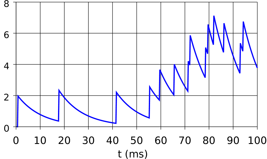
(a) Excitatory potential $V_{2}(t)=V_{\scaleto{\rm E2}{4.4pt}}(t)$.

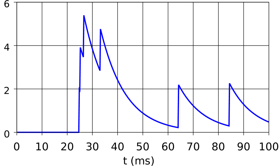
(b) Inhibitory potential $V_{4}(t)=V_{\scaleto{\rm I}{4.4pt}}(t)$.

Figure 1: Filtered shot noise processes.

The following Figures 2 to 5 presents numerical cumulant estimates using closed form expression, and compares them with Monte Carlo simulations run with 10 million samples. Figure 2 presents numerical estimates of first moment and standard deviation, together with the mean obtained by Monte Carlo simulations.

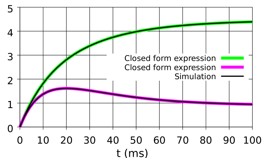
(a) Means of $V_{2}(t)=V_{\scaleto{\rm E2}{4.4pt}}(t)$ and $V_{4}(t)=V_{\scaleto{\rm I}{4.4pt}}(t)$.

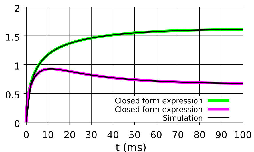
(b) Standard deviations of $V_{\scaleto{\rm E2}{4.4pt}}(t)$ and $V_{\scaleto{\rm I}{4.4pt}}(t)$.

Figure 2: Excitatory and inhibitory means and standard deviations.

Figures 2-3 can be obtained from the Maple commands listed below together with their runtimes on a standard laptop computer, after loading the function definitions listed in Appendix B and the variable assignments of $W$ and $\mu$.

W := $<<10,0,10,10>|<0,10,10,10>|<10,10,0,10>|<0,-8,-8,-10>>$;
mu := [t -> 250, t -> 250, t -> 250, t -> 250]; g := (x, t) -> exp(-100*t + 100*x);
Instruction	Computed quantity	Computation time
c(W, 50, [g], [2], [t], mu)	First cumulant of V2(t)	One second
c(W, 50, [g,g], [4,4], [t,t], mu)	Second cumulant of V4(t)	7 seconds
c(W, 50, [g,g], [4,2], [t,0.05], mu)	Covariance of (V2(t1),V4(t)) for t<t1=0.05	12 seconds
c(W, 50, [g,g], [2,4], [0.05,t], mu)	Covariance of (V2(t1),V4(t)) for t>t1=0.05	15 seconds

Figure 3 presents estimates of the cross-correlations ${\rm Cor}(V_{\scaleto{\rm E2}{4.4pt}}(t),V_{\scaleto{\rm E4}{4.4pt}}(t))$ and ${\rm Cor}(V_{\scaleto{\rm E2}{4.4pt}}(t_{1}),V_{\scaleto{\rm I}{4.4pt}}(t))$ with $t_{1}:=50$ms and $t\in[0,10{\rm ms}]$.

(a) Cross-correlation of $(V_{\scaleto{\rm E2}{4.4pt}}(t),V_{\scaleto{\rm I}{4.4pt}}(t))$.

(b) Cross-correlation of $(V_{\scaleto{\rm E2}{4.4pt}}(t_{1}),V_{\scaleto{\rm I}{4.4pt}}(t))$.

Figure 3: Cross-correlations of $(V_{\scaleto{\rm E2}{4.4pt}}(t),V_{\scaleto{\rm I}{4.4pt}}(t))$ and $(V_{\scaleto{\rm E2}{4.4pt}}(t_{1}),V_{\scaleto{\rm I}{4.4pt}}(t))$ with $t_{1}=50ms$.

Figure 4 presents time-dependent estimates of the third cumulant of $V_{\scaleto{\rm I}{4.4pt}}(t)$ and third joint cumulant of $(V_{\scaleto{\rm E1}{4.4pt}}(t_{1}),V_{\scaleto{\rm E1}{4.4pt}}(t_{1}),V_{\scaleto{\rm I}{4.4pt}}(t))$ with $t_{1}=0.05$, based on the exact moment expressions computed in Maple by the following commands.

Instruction	Computed quantity	Computation time
c(W, 50, [g,g,g], [4,4,4], [t,t,t], mu)	Third cumulant of V4(t)	56 seconds
c(W, 50, [g,g,g], [4,1,1], [t,0.05,0.05], mu)	Third joint cumulant of (V1(t1),V1(t1),V4(t)), t<0.05	239 seconds
c(W, 50, [g,g,g], [1,1,4], [0.05,0.05,t], mu)	Third joint cumulant of (V1(t1),V1(t1),V4(t)), t>0.05	473 seconds

(a) Third cumulant of $V_{4}(t)=V_{\scaleto{\rm I}{4.4pt}}(t)$.

(b) Joint cumulant of $(V_{\scaleto{\rm E1}{4.4pt}}(t_{1}),V_{\scaleto{\rm E1}{4.4pt}}(t_{1}),V_{\scaleto{\rm I}{4.4pt}}(t))$.

Figure 4: Third order cumulants with $t_{1}=50ms$.

Figure 5 presents estimates of the fourth cumulant of $V_{\scaleto{\rm I}{4.4pt}}(t)$ and of the fourth joint cumulant of and $(V_{\scaleto{\rm E1}{4.4pt}}(t),V_{\scaleto{\rm E2}{4.4pt}}(t),V_{\scaleto{\rm E3}{4.4pt}}(t),V_{\scaleto{\rm I}{4.4pt}}(t))$ respectively, computed by the following commands

Instruction	Computed quantity	Computation time
c(W, 50, [g,g,g,g], [4,4,4,4], [t,t,t,t], mu)	Fourth cumulant of V4(t)	677 seconds
c(W, 50, [g,g,g,g], [1,2,3,4], [t,t,t,t], mu)	Fourth joint cumulant of (V1(t),V2(t),V3(t),V4(t))	14917 seconds

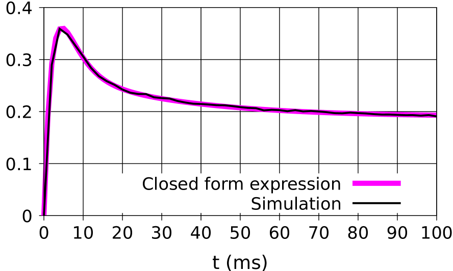
(a) Fourth cumulant of $V_{4}(t)=V_{\scaleto{\rm I}{4.4pt}}(t)$.

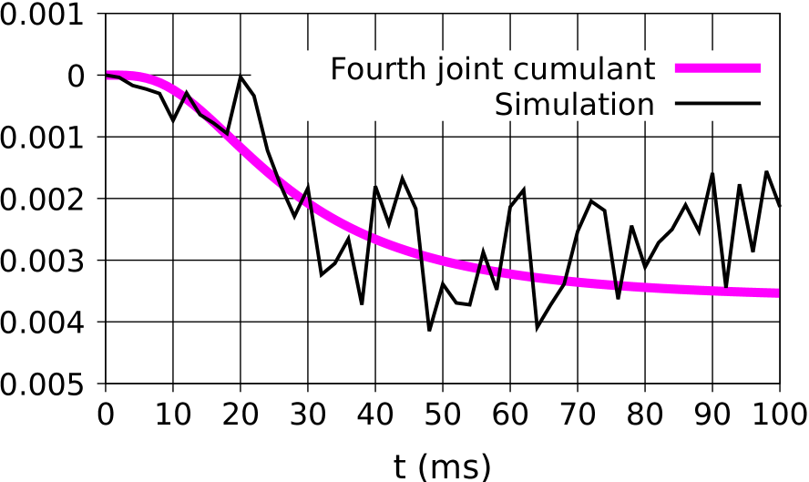
(b) Joint cumulant of $(V_{\scaleto{\rm E1}{4.4pt}}(t),\ldots,V_{\scaleto{\rm E3}{4.4pt}}(t),V_{\scaleto{\rm I}{4.4pt}}(t))$.

Figure 5: Fourth order cumulants.

One can check from Figures 4-$b)$ and 5-$b)$ that the precision of Monte Carlo estimation is degraded starting with joint third cumulants and fourth cumulants, while it becomes clearly insufficient for an accurate estimation of fourth joint cumulants in Figure 5-$b)$. This phenomenon has also been observed in [Pri20] when modeling neuronal activity using Poisson processes, and can be attributed to the fact that the estimation of fourth-order joint cumulants in terms of sampled moments involves a multinomial expression of order four in $4$ variables with changing signs.

The knowledge of cumulants in explicit form also allows us to study their behavior under the variation of other parameters. In Figure 6 we plot the respective evolutions of the first four cumulants of $V_{\scaleto{\rm E2}{4.4pt}}(0.1)$ and $V_{\scaleto{\rm I}{4.4pt}}(0.1)$ as a function of $\alpha W$ with $\alpha\in[0,1]$.

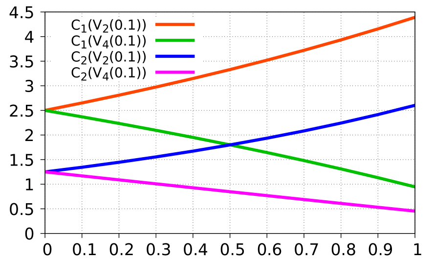
(a) Sensitivities of first and second cumulants.

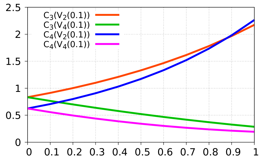
(b) Sensitivities of third and fourth cumulants.

Figure 6: Sensitivities of cumulants.

4 Gram-Charlier expansions

In this section we use our cumulant formulas for the estimation of probability densities of potentials by Gram-Charlier expansions. The Gram-Charlier expansion of the continuous probability density function $\phi_{X}(x)$ of a random variable $X$ is given by

$$\phi_{X}(x)=\frac{1}{\sqrt{\kappa_{2}}}\varphi\left(\frac{x-\kappa_{1}}{\sqrt{\kappa_{2}}}\right)+\frac{1}{\sqrt{\kappa_{2}}}\sum_{n=3}^{\infty}c_{n}H_{n}\left(\frac{x-\kappa_{1}}{\sqrt{\kappa_{2}}}\right)\varphi\left(\frac{x-\kappa_{1}}{\sqrt{\kappa_{2}}}\right),$$ (4.1)

see § 17.6 of [Cra46], where

• $\displaystyle\varphi(x):=\frac{1}{\sqrt{2\pi}}\mathrm{e}^{-x^{2}/2}$, $x\in\real$, is the standard normal density function,

• $\displaystyle H_{n}(x):=\frac{(-1)^{n}}{\varphi(x)}\frac{\partial^{n}\varphi}{\partial x^{n}}(x)$, $x\in\real$, is the Hermite polynomial of degree $n\geq 0$, with $H_{0}(x)=1$, $H_{1}(x)=x$, $H_{3}(x)=x^{3}-3x$, $H_{4}(x)=x^{4}-6x^{2}+3$, $H_{6}(x)=x^{6}-15x^{4}+45x^{2}-15$,

• the sequence $(c_{n})_{n\geq 3}$ is given from the cumulants $(\kappa_{n})_{n\geq 1}$ of $X$ as

  $$c_{n}=\frac{1}{(\kappa_{2})^{n/2}}\sum_{m=1}^{[n/3]}\sum_{\begin{subarray}{c}l_{1}+\cdots+l_{m}=n\\ {l_{1},\ldots,l_{m}\geq 3}\end{subarray}}\frac{\kappa_{l_{1}}\cdots\kappa_{l_{m}}}{m!l_{1}!\cdots l_{m}!},\qquad n\geq 3.$$

In particular, $c_{3}$ and $c_{4}$ can be expressed from the skewness $\kappa_{3}/(\kappa_{2})^{3/2}$ and the excess kurtosis $\kappa_{4}/(\kappa_{2})^{2}$, with

$$c_{3}=\frac{\kappa_{3}}{3!(\kappa_{2})^{3/2}},\quad c_{4}=\frac{\kappa_{4}}{4!(\kappa_{2})^{2}},\quad c_{5}=\frac{\kappa_{5}}{5!\kappa_{5}^{5/2}},\quad\mbox{and}\quad c_{6}=\frac{\kappa_{6}}{6!(\kappa_{2})^{3}}+\frac{(\kappa_{3})^{2}}{2(3!)^{2}(\kappa_{2})^{3}}.$$

Figure 7 presents numerical estimates of skewness and excess kurtosis of $V_{\scaleto{\rm I}{4.4pt}}(t)$ obtained from exact cumulant expressions.

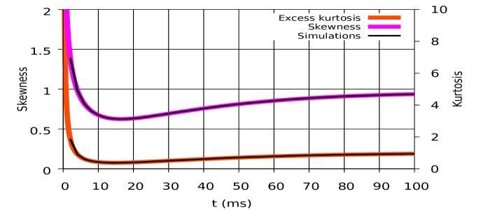
Figure 7: Skewness and kurtosis of $V_{4}(t)=V_{\scaleto{\rm I}{4.4pt}}(t)$.

As above, our results, which are only proved for non-negative weights, remain accurate although the considered Hawkes process allows for inhibition. In what follows, we use third and fourth-order expansions given by

$$\phi_{X}^{(3)}(x)=\frac{1}{\sqrt{\kappa_{2}}}\varphi\left(\frac{x-\kappa_{1}}{\sqrt{\kappa_{2}}}\right)\left(1+c_{3}H_{3}\left(\frac{x-\kappa_{1}}{\sqrt{\kappa_{2}}}\right)\right)$$

and

$$\phi_{X}^{(4)}(x)=\frac{1}{\sqrt{\kappa_{2}}}\varphi\left(\frac{x-\kappa_{1}}{\sqrt{\kappa_{2}}}\right)\left(1+c_{3}H_{3}\left(\frac{x-\kappa_{1}}{\sqrt{\kappa_{2}}}\right)+c_{4}H_{4}\left(\frac{x-\kappa_{1}}{\sqrt{\kappa_{2}}}\right)+c_{6}H_{6}\left(\frac{x-\kappa_{1}}{\sqrt{\kappa_{2}}}\right)\right),$$

and compare them to the first-order expansion

$$\phi_{X}^{(1)}(x)=\frac{1}{\sqrt{\kappa_{2}}}\varphi\left(\frac{x-\kappa_{1}}{\sqrt{\kappa_{2}}}\right)$$

which corresponds to a Gaussian diffusion approximation. Figure 8 presents second, third and fourth-order Gram-Charlier expansions (4.1) for the probability density function of the membrane potential $V_{\scaleto{\rm I}{4.4pt}}(t)$, based on the exact cumulant expressions computed at the times $t=10$ms and $t=20$ms. The purple areas correspond to probability density estimates obtained by Monte Carlo simulations. The second-order expansions correspond to the Gaussian diffusion approximation obtained by matching first and second-order moments.

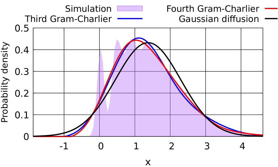
(a) t=10 ms.

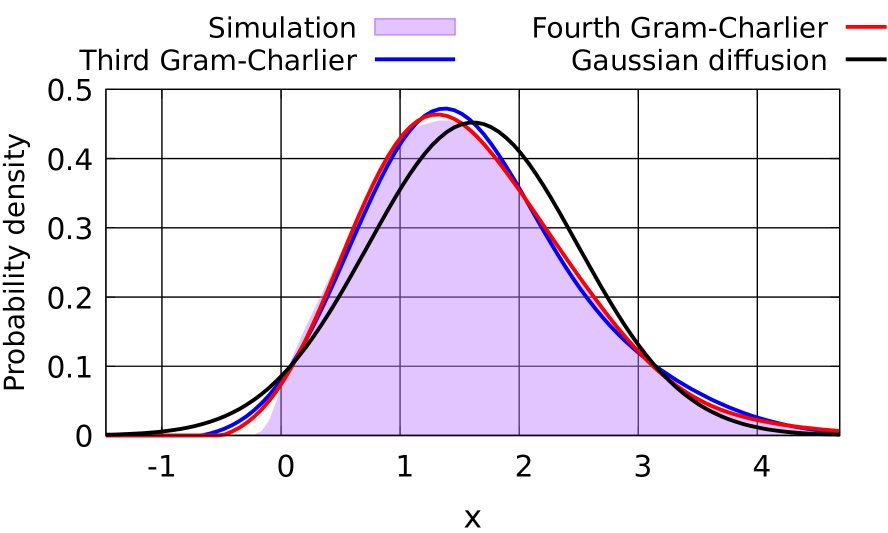
(b) t=20 ms.

Figure 8: Gram-Charlier density expansions vs Monte Carlo density estimation.

Figures 7 and 8 show that the actual probability density estimates obtained by simulation are significantly different from their Gaussian diffusion approximations when skewness and kurtosis take large absolute values. In addition, in Figure 8 the fourth-order Gram-Charlier expansions appear to give the best fit to the actual probability densities, which have negative skewness and positive excess kurtosis, see Figure 7, and the impact of the fourth cumulant remains minimal.

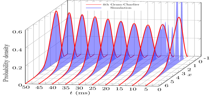
Figure 9: Fourth-order Gram-Charlier expansions vs simulated densities.

Figure 9 presents time-dependent fourth-order Gram-Charlier expansions (4.1), based on exact moment formulas at different times for the probability density function of $V_{\scaleto{\rm I}{4.4pt}}(t)$.

As can be checked from Figure 9, the fourth-order Gram-Charlier expansions fit the purple areas obtained by Monte Carlo simulations. Figure 10-$a)$ compares the Gaussian diffusion (blue) approximation to the fourth-order Gram-Charlier expansion (purple) for the probability density function of $V_{\scaleto{\rm I}{4.4pt}}(t)$ while Figure 10-$b)$ represents the relative difference between the Gaussian diffusion and fourth-order approximations.

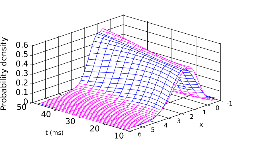
(a) Gaussian diffusion vs $4^{\rm th}$ Gram-Charlier.

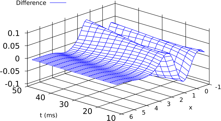
(b) Difference between $2^{\rm nd}$ and $4^{\rm th}$ expansions.

Figure 10: Fourth-order Gram-Charlier expansion vs diffusion approximation.

Conclusion

This paper presents closed-form expressions for the cumulants of arbitrary orders of filtered multivariate Hawkes processes with excitation and inhibition, for application to the modeling of spike trains. Such expressions can be used for the prediction and sensitivity analysis of the statistical behavior of the model over time via immediate numerical evaluations over multiple ranges of parameters, whereas Monte Carlo estimations appear slower and less reliable. They are also used to estimate the probability densities of neuronal membrane potentials using Gram-Charlier density expansions.

Appendix A Proofs of joint cumulant identities

In this section we extend the algorithm of [Pri21, Pri22] for the recursive calculation of the joint cumulants of of Hawkes point processes from the univariate to multivariate setting. We consider a self-exciting point process on $\mathbb{X}:=({}^{d})\times\{1,\ldots,m\}$, $d\geq 1$, with Poisson offspring intensities $\gamma_{i}(dx\times\{i\})=\gamma_{i,j}(dx)=\gamma_{i,j}(x)dx$ and Poisson baseline intensity $\nu(dx\times\{j\})=\nu_{j}(dx)=\nu_{j}(x)dx$ on each copy of ^d, $j=1,\ldots,m$. This process is built in the cluster process framework of [HO74] on the space

$$\Omega=\big{\{}\xi=\{(x,i)\}_{i\in I}\subset\mathbb{X}\ :\ \#(A\cap\xi)<\infty\mbox{ for all compact }A\in{\cal B}(\mathbb{X})\big{\}}$$

of locally finite configurations on $\mathbb{X}$, whose elements $\xi\in\Omega$ are identified with the Radon point measures $\displaystyle\xi(dz)=\sum_{(x,i)\in\xi}\epsilon_{(x,i)}(dz)$, where $\epsilon_{(x,i)}$ denotes the Dirac measure at $(x,i)\in\mathbb{X}$. Any initial point $(x,i)\in\mathbb{X}$ branches into a Poisson random sample on $\mathbb{X}$, denoted by $\xi_{\gamma_{i}}(dz)$, with intensity measure $\gamma_{i,j}(y+dx)$ on every copy of ^d, $i,j=1,\ldots,m$. In case $d=1$ and $\gamma_{i,j}(s)=0$ for $s\leq 0$,

$$N_{t}^{(i)}(\xi):=\xi([0,t]\times\{i\})=\sum_{x\ \!:\ \!(x,i)\in\xi}{\bf 1}_{[0,t]}(x),\qquad i=1,\ldots,m,$$

represents a multivariate Hawkes process with stochastic intensities of the form

$$\lambda^{(i)}_{t}:=\nu+\sum_{j=1}^{m}\int_{0}^{t}\gamma_{i,j}(t-s)dN^{(j)}_{s},\qquad t\in{}_{+},\quad i=1,\ldots,m.$$

For $f$ a sufficiently integrable real-valued function on $\mathbb{X}$, we let

$$G_{(x,i)}(f)=f(x,i)\mathop{\hbox{\rm I\kern-1.99997ptE}}\nolimits_{i}\left[\prod_{(y,j)\in\xi}f(y+x,j)\right]$$

denote the Probability Generating Functional (PGFl) of the branching process $\xi$ given that it is started from a single point at $(x,i)\in\mathbb{X}$. The next proposition states a recursive property for the Probability Generating Functional $G_{(x,i)}(f)$, see also Theorem 1 in [Ada75].

Proposition A.1

The Probability Generating Functional $G_{(x,i)}(f)$ satisfies

$$G_{(x,i)}(f)=f(x,i)\exp\left(\sum_{j=1}^{m}\int_{{}^{d}}(G_{(x+y,j)}(f)-1)\gamma_{i,j}(dy)\right),\qquad(x,i)\in\mathbb{X},$$

and the PGFl of the Hawkes process with Poisson baseline intensity $\nu$ on $\mathbb{X}$ is given by

$$G_{\nu}(f)=\exp\left(\sum_{i=1}^{m}\int_{{}^{d}}(G_{(x,i)}(f)-1)\nu_{i}(x)dx\right).$$

Proof. Viewing the self-exciting point process $\xi$ as a marked point process we have, see e.g. Lemma 6.4.VI of [DVJ03],

$$G_{(x,i)}(f)=f(x,i)\mathop{\hbox{\rm I\kern-1.99997ptE}}\nolimits_{i}\left[\prod_{(y,j)\in\xi}f(y+x,j)\right]$$

$$= f(x,i)\mathop{\hbox{\rm I\kern-1.99997ptE}}\nolimits_{i}\left[\prod_{(y,j)\in\xi_{\gamma_{j}}}\left(\prod_{(z,k)\in\xi}f(z+y+x,k)\right)\right]$$

$$= f(x,i)\mathop{\hbox{\rm I\kern-1.99997ptE}}\nolimits_{i}\left[\prod_{(y,j)\in\xi_{\gamma_{j}}}\mathop{\hbox{\rm I\kern-1.99997ptE}}\nolimits_{j}\left[\prod_{(z,k)\in\xi}f(x+y+z,k)\right]\right]$$

$$= f(x,i)\mathop{\hbox{\rm I\kern-1.99997ptE}}\nolimits_{i}\left[\prod_{(y,j)\in\xi_{\gamma_{j}}}G_{(x+y,j)}(f)\right]$$

$$= \mathrm{e}^{-\gamma_{i}(\mathbb{X})}f(x,i)\sum_{n=0}^{\infty}\frac{1}{n!}\sum_{j_{1},\ldots,j_{n}=1}^{m}\int_{({}^{d})^{n}}G_{(x+y_{1},j_{1})}(f)\cdots G_{(x+y_{n},j_{n})}(f)\gamma_{i,j_{1}}(dy_{1})\cdots\gamma_{i,j_{n}}(dy_{n})$$

$$= f(x,i)\exp\left(\sum_{j=1}^{m}\int_{{}^{d}}(G_{(x+y,j)}(f)-1)\gamma_{i,j}(dy)\right),$$

and

$$G_{\nu}(f) = \mathrm{e}^{-\nu(\mathbb{X})}\sum_{n=0}^{\infty}\frac{1}{n!}\sum_{j_{1},\ldots,j_{n}=1}^{m}\int_{({}^{d})^{n}}G_{(y_{1},j_{1})}(f)\cdots G_{(y_{n},j_{n})}(f)\nu_{j_{1}}(dy_{1})\cdots\nu_{j_{n}}(dy_{n})$$

$$= \exp\left(\sum_{i=1}^{m}\int_{{}^{d}}(G_{(x,i)}(f)-1)\nu_{i}(x)dx\right).$$

$\square$

Let

$$M_{(x,i)}(f):=G_{(x,i)}\big{(}e^{f}\big{)}=\mathop{\hbox{\rm I\kern-1.99997ptE}}\nolimits_{i}\left[\exp\left(f(x,i)+\sum_{(y,j)\in\xi}f(x+y,j)\right)\right]$$

denote the Moment Generating Functional (MGFl) of the random sum $\displaystyle\sum_{(y,j)\in\xi}f(y,j)$ given that the cluster process $\xi$ starts from a single point at $(x,i)\in\mathbb{X}$. The following corollary is an immediate consequence of Proposition A.1, see also Proposition 2.6 in [BD09] for Poisson cluster processes.

Corollary A.2

The Moment Generating Functional $M_{(x,i)}(f)$ satisfies the recursive relation

$$M_{(x,i)}(f)=\exp\left(f(x,i)+\sum_{j=1}^{m}\int_{{}^{d}}(M_{(x+y,j)}(f)-1)\gamma_{i,j}(dy)\right),\qquad(x,i)\in\mathbb{X}.$$ (A.1)

The MGFl of the Hawkes process with baseline intensity $\nu$ on $\mathbb{X}$ is given by

$$M_{\nu}(f)=\exp\left(\sum_{i=1}^{m}\int_{{}^{d}}(M_{(x,i)}(f)-1)\nu_{i}(x)dx\right).$$ (A.2)

Proof of Proposition 2.1. For simplicity, the proof is written using Bell polynomials in the univariate case for $\kappa_{(x,i)}^{(n)}(f):=\kappa_{(x,i)}^{(n)}(f,\ldots,f)$ with $f=f_{1}=\cdots=f_{n}$, and the general case is deduced by polarization. By (A.1), (C.1) and the Faà di Bruno formula (C.2), we have

$$\sum_{n=1}^{\infty}\frac{t^{n}}{n!}\kappa_{(x,i)}^{(n)}(f)=\log M_{(x,i)}(tf)$$

$$=tf(x,i)+\sum_{j=1}^{m}\int_{{}^{d}}\big{(}\mathrm{e}^{\log M_{(x+y,j)}(tf)}-1\big{)}\gamma_{i,j}(dy)$$

$$=tf(x,i)+t\sum_{j=1}^{m}\int_{{}^{d}}\kappa_{(x+y,j)}^{(1)}(f)\gamma_{i,j}(dy)+\sum_{n=2}^{\infty}\frac{t^{n}}{n!}\sum_{j=1}^{m}\int_{{}^{d}}B_{n}\big{(}\kappa_{(x+y,j)}^{(1)}(f),\ldots,\kappa_{(x+y,j)}^{(n)}(f)\big{)}\gamma_{i,j}(dy).$$ (A.3)

At the first order, the expansion (A.3) yields

$$\kappa_{(x,i)}^{(1)}(f) = f(x,i)+\int_{{}^{d}}\sum_{j=1}^{m}\kappa_{(x+y,j)}^{(1)}(f)\gamma_{i,j}(dy)$$

$$= f(x,i)+\sum_{n=1}^{\infty}\sum_{j_{1},\ldots,j_{n}=1}^{m}\int_{{}^{d}}\cdots\int_{{}^{d}}f(x+y_{1}+\cdots+y_{n},j_{n})\gamma_{i,j_{2}}(dy_{1})\cdots\gamma_{j_{n-1},j_{n}}(dy_{n}),$$

while at the order $n\geq 2$ it shows that

$$\kappa_{(x,i)}^{(n)}(f) = \sum_{j=1}^{m}\int_{{}^{d}}B_{n}\big{(}\kappa_{(x+y,i)}^{(1)}(f),\ldots,\kappa_{(x+y,i)}^{(n)}(f)\big{)}\gamma_{i,j}(dy)$$

$$= \big{(}\Gamma\kappa_{(\cdot,\cdot)}^{(n)}(f)\big{)}(x,i)+\big{(}\Gamma\big{(}B_{n}\big{(}\kappa_{(\cdot,\cdot)}^{(1)}(f),\ldots,\kappa_{(\cdot,\cdot)}^{(n)}(f)\big{)}-\kappa_{(\cdot,\cdot)}^{(n)}(f)\big{)}\big{)}(x,i).$$

The above relation rewrites as

$$\big{(}(I-\Gamma)\kappa_{(\cdot,\cdot)}^{(n)}(f)\big{)}(x,i)=\Gamma\big{(}B_{n}\big{(}\kappa_{(\cdot,\cdot)}^{(1)}(f),\ldots,\kappa_{(\cdot,\cdot)}^{(n)}(f)\big{)}-\kappa_{(\cdot,\cdot)}^{(n)}(f)\big{)}(x,i),$$

which yields

$$\kappa_{(x,i)}^{(n)}(f)=\big{(}(I-\Gamma)^{-1}\Gamma\big{(}B_{n}\big{(}\kappa_{(\cdot,\cdot)}^{(1)}(f),\ldots,\kappa_{(\cdot,\cdot)}^{(n)}(f)\big{)}-\kappa_{(\cdot,\cdot)}^{(n)}(f)\big{)}\big{)}(x,i)$$

$$=\sum_{p=1}^{\infty}\sum_{i_{1},\ldots,i_{p}=1}^{m}\int_{{}^{d}}\cdots\int_{{}^{d}}$$

$$\quad\big{(}B_{n}\big{(}\kappa_{(x+x_{1}+\cdots+x_{p},i_{p})}^{(1)}(f),\ldots,\kappa_{(x+x_{1}+\cdots+x_{p},i_{p})}^{(n)}(f)\big{)}-\kappa_{(x+x_{1}+\cdots+x_{p},i_{p})}^{(n)}(f)\big{)}\gamma_{i,i_{1}}(dx_{1})\cdots\gamma_{i_{p-1},i_{p}}(dx_{p})$$

$$=\sum_{p=1}^{\infty}\sum_{i_{1},\ldots,i_{p}=1}^{m}\sum_{k=2}^{n}$$

$$\quad\int_{{}^{d}}\cdots\int_{{}^{d}}B_{n,k}\big{(}\kappa_{(x+x_{1}+\cdots+x_{p},i_{p})}^{(1)}(f),\ldots,\kappa_{(x+x_{1}+\cdots+x_{p},i_{p})}^{(n-k+1)}(f)\big{)}\gamma_{i,i_{1}}(dx_{1})\cdots\gamma_{i_{p-1},i_{p}}(dx_{p}),$$

$n\geq 2$. $\square$

Proof of Corollary 2.2. As above, the proof is only written using Bell polynomials in the case $f=f_{1}=\cdots=f_{n}$. By (C.1), (A.2) and the Faà di Bruno formula (C.2), we have

$$\sum_{n=1}^{\infty}\frac{t^{n}}{n!}\kappa^{(n)}(f) = \log M_{\nu}(tf)$$

$$= \sum_{i=1}^{m}\int_{{}^{d}}(M_{(x,i)}(tf)-1)\nu_{i}(x)dx$$

$$= \sum_{i=1}^{m}\int_{{}^{d}}(\mathrm{e}^{\log M_{(x,i)}(tf)}-1)\nu_{i}(x)dx$$

$$= \sum_{i=1}^{m}\sum_{n=1}^{\infty}\frac{t^{n}}{n!}B_{n}\big{(}\kappa_{(x,i)}^{(1)}(f),\ldots,\kappa_{(x,i)}^{(n)}(f)\big{)}\nu_{i}(x)dx,$$

and therefore

$$\kappa^{(n)}(f)=\sum_{i=1}^{m}\int_{{}^{d}}B_{n}\big{(}\kappa_{(x,i)}^{(1)}(f),\ldots,\kappa_{(x,i)}^{(n)}(f)\big{)}\nu_{i}(x)dx,\qquad n\geq 2.$$

$\square$

Proof of Lemma 2.3. Here we take $d=1$. For all $p,\eta\geq 0$ we have the equalities

$$((I-\Gamma)^{-1}\Gamma e_{p,\eta,t,k})(x,i)$$

$$= \sum_{n=1}^{\infty}\sum_{j_{1},\ldots,j_{n-1}=1}^{m}\int_{[0,t]^{n}}e_{p,\eta,t,k}(x+x_{1}+\cdots+x_{n})\gamma_{i,j_{1}}(dx_{1})\cdots\gamma_{j_{n-1},k}(dx_{n})$$

$$= \sum_{n=1}^{\infty}\frac{[W^{n}]_{i,k}}{(n-1)!}\int_{0}^{t-x}(x+y)^{p}\mathrm{e}^{\eta(x+y)}y^{n-1}\mathrm{e}^{-by}dy$$

$$= \mathrm{e}^{\eta x}\int_{0}^{t-x}(x+y)^{p}[W\mathrm{e}^{yW}]_{i,k}\mathrm{e}^{(\eta-b)y}dy$$

$$= \int_{0}^{t-x}e_{p,\eta,t,k}(x+y)[W\mathrm{e}^{yW}]_{i,k}\mathrm{e}^{-by}dy,\quad x\in[0,t],$$

where we used the fact that the sum $\tau_{1}+\cdots+\tau_{n}$ of $n$ exponential random variables with parameter $b>0$ has a gamma distribution with shape parameter $n\geq 1$ and scaling parameter $b>0$. $\square$

Appendix B Computer codes

The recursion (2.2) and Equation (2.3) can be implemented for any family $(g_{1},\ldots,g_{n})$ of functions defined on ₊ in the following Maple code. The joint cumulants $\langle\langle V_{l_{1}}(t_{1})\cdots V_{l_{n}}(t_{n})\rangle\rangle$, are obtained for $1\leq l_{1},\ldots,l_{n}\leq m$ using the command $\verb|c(W,b,{g1,...,gn},{l1,...,ln},|\\ \verb|{t1,...,tn},mu)|$ in the code below.

⬇

with(LinearAlgebra):

a := proc(y) option remember; return evalf(Multiply(W, MatrixExponential(W, y))); end proc;

h := proc(z, j, W, b, g::list, l::list, t::list) local p, q, r, s, y, i, m, n, k, c; option remember; n := nops(t); if n = 1 then return evalf(g[1](z, t[1])*charfcn[j](l[1]) + int(g[1](z + y, t[1])*exp(-b*y)*a(y)[j, l[1]], y = 0 .. t[1] - z)); end if; s := 0; r := Iterator:-SetPartitions(n); for q in r do p := r:-ToSets(q); if 2 <= nops(p) then for k to Dimension(W)[1] do c := exp(-b*y)*a(y)[j, k]; for i to nops(p) do c := c*h(z + y, k, W, b, map(op, convert(p[i], list), g), map(op, convert(p[i], list), l), map(op, convert(p[i], list), t)); end do; s := s + c; end do; end if; end do; return int(s, y = 0 .. t[1] - z); end proc;

c := proc(W, b, g::list, l::list, t::list, mu::list) local y, e, p, q, r, s, i, j, m, n; option remember; n := nops(t); s := 0; for j to Dimension(W)[1] do s := s + mu[j](y)*h(y, j, W, b, g, l, t); if 2 <= n then r := Iterator:-SetPartitions(n); for q in r do p := r:-ToSets(q); if 2 <= nops(p) then e := 1; for i to nops(p) do e := e*h(y, j, W, b, map(op, convert(p[i], list), g), map(op, convert(p[i], list), l), map(op, convert(p[i], list), t)); end do; s := s + mu[j](y)*e; end if; end do; end if; end do; return int(s, y = 0 .. t[1]); end proc;

Joint moments can be computed in Maple using the command $\verb|m(W,b,{g1,....,gn},{jl,|$
$\verb|...,jl},{t1,...,tn},mu)|$ defined in the following code.

⬇

m := proc(W, b, f::list, l::list, t::list, mu::list) local e, u, p, q, r, s, i, n; option remember; n := nops(t); s := c(W, b, f, l, t, mu); if 2 <= n then r := Iterator:-SetPartitions(n); for q in r do p := r:-ToSets(q); if 2 <= nops(p) then e := 1; for i to nops(p) do e := e*c(W, b, map(op, convert(p[i], list), f), map(op, convert(p[i], list), l), map(op, convert(p[i], list), t), mu); end do; s := s + e; end if; end do; end if; return s; end proc;

Alternatively, the computation of joint cumulants can be carried out using the command $\verb|c[W,b,[g1,...,gn],[l1,...,ln],[t1,...,tn],mu]|$ in the following Mathematica codes.

⬇

Needs["Combinatorica`"]

a[y_] := W . MatrixExp[y*W];

h[z_, j_Integer, W_, b_, g__, l__, t__] := h[z, j, W, b, g, l, t] = (Module[{y, k, i, c, n, m, s}, n = Length[t]; If[n == 1, Return[g[[1]][z, t[[1]]]*Boole[j == l[[1]]] + Integrate[g[[1]][z + y, t[[1]]]*E^(-b*y)*a[y][[j, l[[1]]]], {y, 0, t[[1]] - z}]]]; s = 0; Do[c = 1; If[Length[p] >= 2, For[i = 1, i <= Length[p], i++, c *= Block[{u = y + z, w = g[[p[[i]]]], r = l[[p[[i]]]], v = t[[p[[i]]]]}, h[u, k, W, b, w, r, v]]]; s += c], {p, SetPartitions[n]}]; Return[Sum[Integrate[E^(-b*y)*a[y][[j, k]]*s, {y, 0, t[[1]] - z}], {k, 1, Dimensions[W][[1]]}]]]);

c[W_, b_, g__, l__, t__, mu_] := (Module[{y, e, n, i, j, m, s}, n = Length[g]; s = 0; For[j = 1, j <= Dimensions[W][[1]], j++, Do[e = mu[y][[j]]; For[i = 1, i <= Length[p], i++, e *= Block[{u = y, w = g[[p[[i]]]], r = l[[p[[i]]]], v = t[[p[[i]]]]}, h[u, j, W, b, w, r, v]]]; s += Flatten[{e}][[1]], {p, SetPartitions[n]}]]; Return[Integrate[s, {y, 0, t[[1]]}]]]);

Figures 2 to 5 can also been plotted from the following Mathematica commands.

W := $\{\{$10, 0, 10, 0$\}$, $\{$ 0, 10, 10, -8 $\}$, $\{$ 10, 10, 0, -8 $\}$, $\{$ 10, 10, 10, -10$\}\}$;
g[u_, t_] := E^(-(t - u)/0.01); mu[t_] := $\{$ 250, 250, 250, 250 $\}$;
Instruction	Computed quantity	Computation time
c[W, 50, $\{$g$\}$, $\{$2$\}$, $\{$t$\}$, mu]	First cumulant of V2(t)	One second
c[W, 50, $\{$g,g$\}$, $\{$4,4$\}$, $\{$t,t$\}$, mu]	Second cumulant of V4(t)	122 seconds
c[W, 50, $\{$g,g$\}$, $\{$4,2$\}$, $\{$t,0.05$\}$, mu]	Covariance of (V2(t1),V4(t)) for t<t1=0.05	250 seconds
c[W, 50, $\{$g,g$\}$, $\{$2,4$\}$, $\{$0.05,t$\}$, mu]	Covariance of (V2(t1),V4(t)) for t>t1=0.05	250 seconds
c[W, 50, $\{$g,g,g$\}$, $\{$4,4,4$\}$, $\{$t,t,t$\}$, mu]	Third cumulant of V4(t)	3057 seconds
c[W, 50, $\{$g,g,g$\}$, $\{$4,1,1$\}$, $\{$t,0.05,0.05$\}$, mu]	Third joint cumulant of (V1(t1),V1(t1),V4(t)), t<t1=0.05
c[W, 50, $\{$g,g,g$\}$, $\{$1,1,4$\}$, $\{$0.05,0.05,t$\}$, mu]	Third joint cumulant of (V1(t1),V1(t1),V4(t1)), t>t1=0.05
c[W, 50, $\{$g,g,g,g$\}$, $\{$4,4,4,4$\}$, $\{$t,t,t,t$\}$, mu]	Fourth cumulant of V4(t)
c[W, 50, $\{$g,g,g,g$\}$, $\{$1,2,3,4$\}$, $\{$t,t,t,t$\}$, mu]	Fourth joint cumulant of (V1(t),V2(t),V3(t),V4(t))

Standard moments of order $n\geq 1$ can be computed in Mathematica using the command $\verb|m[W,b,[g1,...,gn],[l1,...,ln],[t1,...,tn],mu]|$ defined below.

⬇

m[W_, b_, g__, l__, t__, mu_] := (Module[{n, e, i, s}, s = 0; n = Length[t]; If[n == 0, Return[1]]; Do[e = 1; For[i = 1, i <= Length[pp], i++, e *= c[W, b, g[[pp[[i]]]], l[[pp[[i]]]], t[[pp[[i]]]], mu]]; s += e, {pp, SetPartitions[n]}]; Flatten[{s}][[1]]]);

Appendix C Joint cumulants and Faà di Bruno formula

We refer to e.g. [Luk55] or [McC87] for the background combinatorics recalled in this section. The joint cumulants of orders $(l_{1},\ldots,l_{n})$ of a random vector $X=(X_{1},\ldots,X_{n})$, $1\leq l_{1},\ldots,l_{n}\leq m$, are the coefficients $\langle\langle X_{1}^{l_{1}}\cdots X_{n}^{l_{n}}\rangle\rangle$ appearing in the log-moment generating (MGF) expansion

$$\log\langle\mathrm{e}^{t_{1}X_{1}+\cdots+t_{n}X_{n}}\rangle=\sum_{l_{1},\ldots,l_{n}\geq 1}\frac{t^{l_{1}}_{1}\cdots t^{l_{n}}_{n}}{l_{1}!\cdots l_{n}!}\langle\langle X_{1}^{l_{1}}\cdots X_{n}^{l_{n}}\rangle\rangle,$$ (C.1)

for $(t_{1},\ldots,t_{n})$ in a neighborhood of zero in ⁿ. Recall that if $f(t)$ admits the formal series expansion

$$f(t)=\sum_{n=1}^{\infty}\frac{a_{n}}{n!}t^{n},$$

by the Faà di Bruno formula we have

$$\mathrm{e}^{f(t)}-1=\sum_{n=1}^{\infty}\frac{t^{n}}{n!}B_{n}(a_{1},\ldots,a_{n}),$$ (C.2)

where

$$B_{n}(a_{1},\ldots,a_{n})=\sum_{k=1}^{n}B_{n,k}(a_{1},\ldots,a_{n-k+1})$$

is the complete Bell polynomial of degree $n\geq 1$, and

$$B_{n,k}(a_{1},\ldots,a_{n-k+1})=\sum_{\pi_{1}\cup\cdots\cup\pi_{k}=\{1,\ldots,n\}}a_{|\pi_{1}|}(X)\cdots a_{|\pi_{k}|}(X),\qquad 1\leq k\leq n,$$

is the partial Bell polynomial of order $(n,k)$, where the sum runs over the partitions $\pi_{1},\ldots,\pi_{k}$ of the set $\{1,\ldots,n\}$, and $|\pi_{i}|$ denotes the cardinality of $\pi_{i}$. Joint moments can be obtained from the joint moment-cumulant relation

$$\langle V_{l_{1}}(t_{1})\cdots V_{l_{n}}(t_{n})\rangle=\sum_{\pi\in\Pi[n]}\prod_{j=1}^{|\pi|}\left<\left<\prod_{i\in\pi_{j}}V_{l_{i}}(t_{i})\right>\right>,$$ (C.3)

where the above sum is over the set $\Pi[n]$ of partitions $\pi$ of $\{1,\ldots,n\}$. Joint cumulants can also be recovered from joint moments from the relation

$$\langle\langle V_{l_{1}}(t_{1})\cdots V_{l_{n}}(t_{n})\rangle\rangle=\sum_{\pi\in\Pi[n]}({|\pi|}-1)!(-1)^{{|\pi|}-1}\prod_{j=1}^{|\pi|}\left<\prod_{i\in\pi_{j}}V_{l_{i}}(t_{i})\right>,$$

where the above sum is over the set $\Pi[n]$ of partitions $\pi$ of $\{1,\ldots,n\}$, which can be obtained by Möbius inversion of the moment-cumulant relation (C.3).

References

[Ada75]
L. Adamopoulos.
Some counting and interval properties of the mutually-exciting
processes.
J. Appl. Probab., 12(1):78–86, 1975.
[AI01]
K.-I. Amemori and S. Ishii.
Gaussian process approach to spiking neurons for inhomogeneous
Poisson inputs.
Neural Comput., 13:2763–2797, 2001.
[BD09]
L. Bogachev and A. Daletskii.
Poisson cluster measures: Quasi-invariance, integration by parts
and equilibrium stochastic dynamics.
J. Funct. Anal., 256:432–478, 2009.
[BD15]
M. Brigham and A. Destexhe.
Nonstationary filtered shot-noise processes and applications to
neuronal membranes.
Phys. Rev. E, 91:062102, 2015.
[BDM12]
E. Bacry, K. Dayri, and J.F. Muzy.
Non-parametric kernel estimation for symmetric Hawkes processes.
Application to high frequency financial data.
Eur. Phys. J. B, 85:157–168, 2012.
[Bur06a]
A. N. Burkitt.
A review of the integrate-and-fire neuron model: I. Homogeneous
synaptic input.
Biol. Cybernetics, 95:1–19, 2006.
[Bur06b]
A. N. Burkitt.
A review of the integrate-and-fire neuron model: II.
Inhomogeneous synaptic input and network properties.
Biol. Cybernetics, 95:97–112, 2006.
[Che16]
Y. Chen.
Multivariate Hawkes processes and their simulations.
Preprint, 7 pages, 2016.
[CHY20]
L. Cui, A. Hawkes, and H. Yi.
An elementary derivation of moments of Hawkes processes.
Adv. in Appl. Probab., 52:102–137, 2020.
[CR10]
S. Cardanobile and S. Rotter.
Multiplicatively interacting point processes and applications to
neural modeling.
Journal of Computational Neuroscience, 28:267–284, 2010.
[Cra46]
H. Cramér.
Mathematical methods of statistics.
Princeton University Press, Princeton, NJ, 1946.
[CTRM06]
D. Cai, L. Tao, A.V. Rangan, and D. W. McLaughlin.
Kinetic theory for neuronal network dynamics.
Comm. Math. Sci., 4(1):97–127, 2006.
[CXVK19]
Y. Chen, Q. Xin, V. Ventura, and R. E Kass.
Stability of point process spiking neuron models.
Journal of Computational Neuroscience, 46(1):19–32, 2019.
[DP22]
A. Daw and J. Pender.
Matrix calculations for moments of Markov processes.
Preprint arXiv:1909.03320, to appear in Advances in Applied
Probability, 2022.
[DVJ03]
D. J. Daley and D. Vere-Jones.
An introduction to the theory of point processes. Vol. I.
Probability and its Applications. Springer-Verlag, New York, 2003.
[DZ11]
A. Dassios and H. Zhao.
A dynamic contagion process.
Adv. in Appl. Probab., 43:814–846, 2011.
[GDT17]
F. Gerhard, M. Deger, and W. Truccolo.
On the stability and dynamics of stochastic spiking neuron models:
Nonlinear Hawkes process and point process GLMs.
PLoS Comput Biol, 13(2):1–31, 2017.
[Haw71]
A.G. Hawkes.
Spectra of some self-exciting and mutually exciting point processes.
Biometrika, 58:83–90, 1971.
[HO74]
A.G. Hawkes and D. Oakes.
A cluster process representation of a self-exciting process.
J. Appl. Probab., 11(3):493–503, 1974.
[JHR15]
S. Jovanović, J. Hertz, and S. Rotter.
Cumulants of Hawkes point processes.
Phys. Rev. E, 91, 2015.
[KAR04]
A. Kuhn, A. Aertsen, and S. Rotter.
Neuronal integration of synaptic input in the fluctuation-driven
regime.
J. Neurosci., 24(10):2345–2356, 2004.
[KR20]
M. Kordovan and S. Rotter.
Spike train cumulants for linear-nonlinear Poisson cascade models.
Preprint arXiv:2001.05057 [q-bio.NC], 2020.
[KRS10]
M. Krumin, I. Reutsky, and S. Shoham.
Correlation-based analysis and generation of multiple spike trains
using Hawkes models with an exogenous input.
Frontiers in Computational Neuroscience, 4:12, 2010.
[Luk55]
E. Lukacs.
Applications of Faà di Bruno’s formula in mathematical
statistics.
Amer. Math. Monthly, 62:340–348, 1955.
[McC87]
P. McCullagh.
Tensor methods in statistics.
Monographs on Statistics and Applied Probability. Chapman & Hall,
London, 1987.
[Oga81]
Y. Ogata.
On Lewis’ simulation method for point processes.
IEEE Trans. Inform. Theory, IT-27(1):23–31, 1981.
[OJSBB17]
G.K. Ocker, K. Josić, E. Shea-Brown, and M.A. Buice.
Linking structure and activity in nonlinear spiking networks.
PLoS Comput Biol, 16(3):1–47, 2017.
[Pri20]
N. Privault.
Nonstationary shot-noise modeling of neuron membrane potentials by
closed-form moments and Gram-Charlier expansions.
Biol. Cybernetics, 114:499–518, 2020.
[Pri21]
N. Privault.
Recursive computation of the Hawkes cumulants.
Statist. Probab. Lett., 177:Article 109161, 2021.
[Pri22]
N. Privault.
An algorithm for the computation of joint Hawkes moments with
exponential kernel.
In Proceedings of the 53rd ISCIE International Symposium on
Stochastic Systems Theory and Its Applications (SSS’21), pages 1–8, 2022.
[RBRTM13]
P. Reynaud-Bouret, V. Rivoirard, and C. Tuleau-Malot.
Inference of functional connectivity in neurosciences via Hawkes
processes.
In 2013 IEEE Global Conference on Signal and Information
Processing, pages 317–320. IEEE Press, 2013.
[RD05]
M. Rudolph and A. Destexhe.
An extended analytic expression for the membrane potential
distribution of conductance-based synaptic noise.
Neural Comput., 17:2301, 2005.
[RG05]
M. Richardson and W. Gerstner.
Synaptic shot noise and conductance fluctuations affect the membrane
voltage with equal significance.
Neural Comput., 17:923–947, 2005.
[Tuc88]
H.C. Tuckwell.
Introduction to Theoretical Neurobiology: Volume 2, Nonlinear
and Stochastic Theories.
Cambridge University Press, Cambridge, 1988.
[VD74]
A. Verveen and L. DeFelice.
Membrane noise.
Progress in Biophysics and Molecular Biology, 28:189–234,
1974.
[WL08]
L. Wolff and B. Lindner.
Method to calculate the moments of the membrane voltage in a model
neuron driven by multiplicative filtered shot noise.
Phys. Rev. E, 77:041913, 2008.
[WL10]
L. Wolff and B. Lindner.
Mean, variance, and autocorrelation of subthreshold potential
fluctuations driven by filtered conductance shot noise.
Neural Comput., 22:94–120, 2010.