Defining Canonical Momenta for Discretised SU$(2)$ Gauge Fields

Abstract

In this proceeding contribution we discuss how to define canonical momenta for SU$(N)$ lattice gauge theories in the Hamiltonian formalism in a basis where the gauge field operators are diagonal. For an explicit discretisation of SU$(2)$ we construct the momenta and check the violation of the fundamental commutation relations.

1 Introduction

The Hamiltonian of lattice gauge theories was formulated by Kogut and Susskind in Ref. [1] already in 1974. For an SU$(N)$ lattice gauge theory it reads in generic form

$$\hat{H}=\ \frac{g_{0}^{2}}{4}\sum_{\mathbf{x},c,k}\left(\hat{L}_{c,k}^{2}(\mathbf{x})+\hat{R}_{c,k}^{2}(\mathbf{x})\right)+\frac{1}{2g_{0}^{2}}\sum_{\mathbf{x},k<l}\mathrm{Tr}\,\mathrm{Re}\,\hat{P}_{kl}(\mathbf{x})\,,$$ (1)

with $g_{0}$ the (bare) gauge coupling constant and the lattice spacing set to $a=1$. Note that without discretised gauge fields $\hat{L}^{2}$ and $\hat{R}^{2}$ are identical. Here, $\mathbf{x}$ are the coordinates in a $n$-dimensional, spatial lattice with lattice spacing $a$

$$\Lambda\ =\ \{\mathbf{x}:x_{k}=0,a,2a,\ldots,(L-1)a\}\,,$$

with periodic boundary conditions and $k=1,2,\ldots,n$. $c$ labels the colour index of the group SU$(N)$. The trace is taken in colour space and $\hat{P}_{kl}(x)$ are plaquette operators

$$\hat{P}_{kl}(\mathbf{x})\ =\ \hat{U}_{k}(\mathbf{x})\,\hat{U}_{l}(\mathbf{x}+\hat{k})\,\hat{U}^{\dagger}_{k}(\mathbf{x}+\hat{l})\,\hat{U}^{\dagger}_{l}(\mathbf{x})\,,$$

with $\hat{k}$ a vector of length $a$ in direction $k$. The elements $\hat{u}_{ij}:\mathcal{H}\to\mathcal{H}$ of $\hat{U}_{k}\in\mathrm{SU}(N)$ represent the gauge field operators in direction $k$ and the $\hat{L}_{x,k}$ and $\hat{R}_{c,k}$ are the corresponding canonical momenta. In the following the spatial coordinates $\mathbf{x}$ and the directions will not be relevant and, thus, we will drop them.

Given the generators $t_{c}$ of the group SU$(N)$, the elements of the $\hat{U}$ and their canonical momenta are defined via the commutation relation

$$[\hat{L}_{c},\hat{U}_{mn}]\ =\ (t_{c})_{mj}\,\hat{U}_{jn}\,,\qquad[\hat{R}_{c},\hat{U}_{mn}]\ =\ \hat{U}_{mj}(t_{c})_{jn}\,.$$ (2)

Moreover, the $\hat{L}_{c}$ resemble the group structure

$$[\hat{L}_{a},\hat{L}_{b}]=f_{abc}\hat{L}_{c}\,,$$ (3)

with the the structure constants $f_{abc}$ of the corresponding Lie algebra, and likewise the $\hat{R}_{c}$.

If this formalism is to be implemented using tensor networks or on future digital quantum computers, a discretisation scheme is needed with a corresponding truncation scheme for the Hilbert space. And the race is on to find the most efficient way to implement this discretisation. For different schemes on the market see for instance Ref. [2].

Most of the existing discretisations of the Hamiltonian have in common that they work in a basis where the kinetic / electric part of $\hat{H}$ is diagonal. The magnetic part is then obtained for instance by a character expansion. In this proceeding we explore the possibility to work in a basis where the gauge field operators are diagonal: this might be advantageous in particular regions of parameter space, see Refs. [3, 4] for a discussion in Abelian U$(1)$ theory.

2 State Space

To simplify the discussion and to be concrete, we resort to the special case of SU$(2)$ in the following with generators given by the Pauli matrices and colour indices $c=1,2,3$. We will chose states $|U\rangle\in\mathcal{H}$ in a Hilbert space $\mathcal{H}$ which are eigenstates of the operators $\hat{U}$ in the following sense: parametrise an SU$(2)$ matrix using three real valued parameters $y_{0},y_{1},y_{2}$ with

$$\begin{pmatrix}y_{0}+\mathrm{i}y_{1}&y_{2}+\mathrm{i}y_{3}\\ -y_{2}+\mathrm{i}y_{3}&y_{0}-\mathrm{i}y_{1}\\ \end{pmatrix}\in\mathrm{SU}(2)\,,\qquad y_{3}^{2}=1-\sum_{i=0}^{2}y_{i}^{2}\,.$$

Now define operators $\hat{y}_{j}:\mathcal{H}\to\mathcal{H}$ by the following action

$$\hat{y}_{j}|U\rangle\ =\ y_{j}|U\rangle\,.$$

Defining also

$$\begin{split}\hat{u}_{00}=\hat{y}_{0}+\mathrm{i}\hat{y}_{1}\,,\quad\hat{u}_{01}=\hat{y}_{2}+\mathrm{i}\hat{y}_{3}\,,\\ \hat{u}_{10}=-\hat{y}_{2}+\mathrm{i}\hat{y}_{3}\,,\quad\hat{u}_{11}=\hat{y}_{0}-\mathrm{i}\hat{y}_{1}\,,\\ \end{split}$$

we can set for $\hat{U}:\mathcal{H}\to\mathcal{H}$

$$\hat{U}=\begin{pmatrix}\hat{u}_{00}&\hat{u}_{01}\\ \hat{u}_{10}&\hat{u}_{11}\\ \end{pmatrix}\,.$$

Therefore, the $y_{1,2,3}$ can be regarded as quantum numbers labelling the states $|U\rangle$ which are simultaneous eigenstates of operators $\hat{y}_{1,2,3}$.

Formally, we can define the momenta as Lie derivatives:

$$\hat{L}_{c}\,f(\hat{U})\ =-\mathrm{i}\frac{\mathrm{d}}{\mathrm{d}\alpha}\,f\left(e^{\mathrm{i}\,\alpha t_{c}}\,\hat{U}\right)|_{\alpha=0}\,,\qquad\hat{R}_{c}\,f(\hat{U})\ =-\mathrm{i}\frac{\mathrm{d}}{\mathrm{d}\alpha}\,f\left(\hat{U}\,e^{\mathrm{i}\,\alpha t_{c}}\right)|_{\alpha=0}$$ (4)

for a function $f(\hat{U})$.

We make the Hilbert space finite by using one of the partitionings we proposed in Ref. [5]. These partitionings define a finite set of group elements $G_{\mathrm{M}}=\{y(\mu):\mu=1,\ldots,N(M)\}$, which are asymptotically isotropic and dense in SU$(2)$ depending on a parameter $M\in\mathbb{N}$. The continuum group is approached with $M\to\infty$. The mean distance roughly goes like $1/M$ and the number of elements $N(M)\sim M^{3}$.

3 Discretising the derivative in SU$(2)$

With one of the aforementioned partitionings the discretisation of the operators $\hat{U}$ and the state space is straightforward. However, the discretisation of the canonical momenta is more involved. The finite difference operation

$$\begin{split}\frac{1}{\alpha}\left(f(e^{\mathrm{i}\alpha t_{a}}\,\hat{U})-f(\hat{U})\right)\ &=\ \frac{1}{\alpha}\left(f(\hat{U})+\alpha\hat{L}_{a}f(\hat{U})-f(\hat{U})+O(\alpha^{2})\right)\\ &=\ \hat{L}_{a}f(\hat{U})\,+O(\alpha)\end{split}$$ (5)

in direction $a$ is a natural way to implement the discretisation. Thus, we need to reconstruct the directional derivative from the existing neighbouring elements in $G_{\mathrm{M}}$. Let $U\in G_{\mathrm{M}}$ be one element for which we desire to define $\hat{L}_{a}$. Let us chose a specific representation and $f(\hat{U})=\hat{U}$. Then, one can find three neighbours $V_{i}\,,\ i=1,2,3$ of this element $U$. Moreover, there are three $W_{i}\in\mathrm{SU}(2)$

$$V_{i}(U)=W_{i}\,U\qquad\Leftrightarrow\qquad W_{i}=V_{i}U^{-1}=\exp(\mathrm{i}\alpha_{b}^{i}t_{b})$$ (6)

with $\alpha_{b}^{i}\in\mathbb{R}$, $b=1,2,3$ and $i=1,2,3$. Now, with additional real parameters $\gamma_{i}\in\mathbb{R}$ we can expand as follows

$$\begin{split}\gamma_{1}W_{1}U+\gamma_{2}W_{2}U+\gamma_{3}W_{3}U&\approx\left(\gamma_{1}(1+\mathrm{i}\alpha_{b}^{1}t_{b})+\gamma_{2}(1+\mathrm{i}\alpha_{b}^{2}t_{b})+\gamma_{3}(1+\mathrm{i}\alpha_{b}^{3}t_{b})\right)U\\ &=\sum_{i}\gamma_{i}U+\mathrm{i}\sum_{i,b}\gamma_{i}\alpha_{b}^{i}t_{b}U\,.\end{split}$$

Therefore, one needs to determine the parameters $\gamma_{i}$ such that

$$\sum_{i,b}\gamma_{i}\alpha_{b}^{i}t_{b}=t_{a}\,,$$ (7)

because then

$$\begin{split}-\left(\sum_{i=1}^{n}\gamma_{i}\right)U&+\gamma_{1}V_{1}+\gamma_{2}V_{2}+\gamma_{3}V_{3}\\ &=-\left(\sum\gamma_{i}\right)U+\gamma_{1}W_{1}U+\gamma_{2}W_{2}U+\gamma_{3}W_{3}U\\ &\approx\mathrm{i}\left(\gamma_{1}\alpha_{b}^{1}t_{b}+\gamma_{2}\alpha_{b}^{2}t_{b}+\gamma_{3}\alpha_{b}^{3}t_{b}\right)U\\ &=\mathrm{i}t_{a}U\,.\end{split}$$

Thus, the algorithm reads

1. find three next neighbours $V_{i}\in G_{\mathrm{M}}$ of one element $U\in G_{\mathrm{M}}$, then compute the $W_{i}$ as defined above and the three vectors $\alpha_{b}\in\mathbb{R}^{3}$.

2. combine the column vectors $\alpha_{b}$ into a $3\times 3$ matrix and solve

   $$e_{a}=\gamma\cdot(\alpha_{1}\alpha_{2}\alpha_{3})$$

   for vector $\gamma\in\mathbb{R}^{3}$ with $e_{a}\in\mathbb{R}^{3}$ the unit vector in direction $a$.

3. the only non-zero elements of the discrete operator $\hat{L}_{a}\in\mathbb{R}^{N(M)\times N(M)}$ are then given by

   $$(\hat{L}_{a})_{\#U,\,\#V_{i}(U)}=\gamma_{i}\,,\qquad(\hat{L}_{a})_{\#U,\,\#U}=-\sum_{i}\gamma_{i}$$

   with $\#V_{i}(U)$ the index of $V_{i}(U)$ and $\#U$ the index of $U$ in $G_{\mathrm{M}}$.

For determining also $R_{a}$ the algorithm only needs to be modified by replacing eq. 6 by

$$V_{i}=UW_{i}\,,\quad\Leftrightarrow\quad W_{i}=U^{-1}V_{i}\,.$$

4 Test of the Commutation Relations

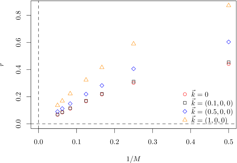
Figure 1: We plot $r$ for the commutator eq. 9 as defined in the text as a function of $1/M$ for different Fourier vectors $\vec{k}$.

For the test of this discretisation we check whether the commutation relations eqs. 2 and 3 are approximately fulfilled by the discretised operators defined above. For this purpose we chose what we call linear partitioning in Ref. [5], which is defined by the following set of points

$$\begin{split}G_{\mathrm{M}}&\coloneqq\left\{\frac{1}{J}\left(s_{0}j_{0},\dots,s_{3}j_{3}\right)\right.\\ &\left|\,\sum_{i=0}^{3}j_{i}=M,\;\forall i\in\{0,\dots,3\}:\,s_{i}\in\{\pm 1\},\,j_{i}\in\mathbb{N}\right\}\,,\end{split}$$ (8)

with

$$J\coloneqq\sqrt{\sum_{i=0}^{3}j_{i}^{2}}\,.$$

This is directly related to the aforementioned parametrization of SU$(2)$ via $(s_{0}j_{0},s_{1}j_{1},s_{2}j_{2},s_{3}j_{3})/J\equiv(y_{0},y_{1},y_{2},y_{3})$.

With the above definitions of $\hat{L}$ and $\hat{R}$ it is ensured that if applied to a constant vector one obtains zero. Much like in the one dimensional case of a finite difference operator, we expect $\hat{L}$ and $\hat{R}$ to work best if applied to slowly varying vectors in the algebra. This is why we define the equivalent of Fourier modes in the algebra denoted by $v(\vec{k})$. Since the convergence is correct to $O(\alpha)$ for each element of $G_{\mathrm{M}}$ separately, we compute

$$z\ =\ \left([L_{a},U_{jl}]-(t_{a})_{ji}U_{il}\right)\cdot v(\vec{k})$$ (9)

and then the mean deviation as

$$r\ =\ \frac{1}{N(M)}\sum|z_{i}|$$ (10)

with $N(M)$ the number of points in the set $G_{\mathrm{M}}$. Note that one could equivalently use

$$r^{\prime}=\frac{\langle v|z\rangle}{\langle v|v\rangle}\,.$$

In fig. 1 we show the result of our test for different Fourier vectors $\vec{k}$ by plotting $r$ as a function of $1/M$. One can observe that $|r|$ increases at fixed $M$ with the modulus of $\vec{k}$. Moreover, for all vectors $\vec{k}$ we see convergence of $r\to 0$ with $M\to\infty$. We also note that the average deviation is not particularly small for the $M$-values considered here.

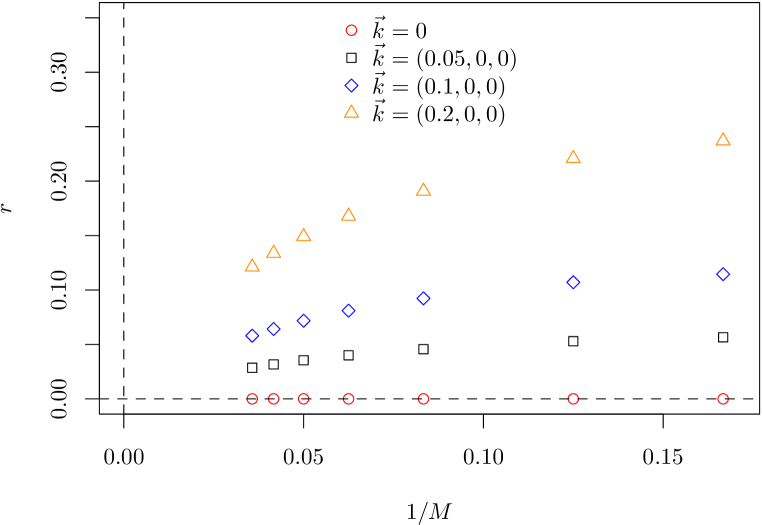
Figure 2: We plot $r$ for the commutator eq. 11 as defined in the text as a function of $1/M$ for different Fourier vectors $\vec{k}$.

In fig. 2 we again show $r$ as a function of $1/M$, but this time we define

$$z\ =\ \left([L_{a},L_{b}]\ +\ 2\mathrm{i}\,\epsilon_{abc}\,L_{c}\right)\cdot v(\vec{k})$$ (11)

with the appropriate $f_{abc}$ for SU$(2)$. Note that the scale of the $x$-axis is different compared to fig. 1 and also the Fourier vectors are different with smaller $|\vec{k}|$-values than in fig. 1.

First of all, for $\vec{k}=0$, $r$ vanishes independently of $M$. This is due to the fact that $L_{a}v(0)=0$ per construction. We observe that for this commutator the convergence appears to be slower: only at $1/M<0.2$ convergence towards zero becomes plausible, even though probably at least a factor two larger values of $M$ are needed to reliably establish this observation.

5 Summary and Outlook

In this proceeding contribution we have discussed how to define canonical momenta for discretised SU$(N)$ gauge fields. We have tested our discretisation scheme with one particular gauge group discretisation and we observe that in the limit of continuous group the exact commutation relations are recovered. The particular construction discussed here for SU$(2)$ can be generalised to SU$(3)$.

The obvious next steps are the investigation of the spectrum of the free theory using the discretised momenta and to compare to other discretisation schemes. And, of course, an implementation of the Hamiltonian for a digital quantum computer must be explored.

References

- [1] J. B. Kogut and L. Susskind, Phys. Rev. D 11, 395 (1975).
- [2] Z. Davoudi, I. Raychowdhury and A. Shaw, Phys. Rev. D 104, 074505 (2021), arXiv:2009.11802 [hep-lat].
- [3] D. Paulson et al., PRX Quantum 2, 030334 (2021), arXiv:2008.09252 [quant-ph].
- [4] J. F. Haase et al., Quantum 5, 393 (2021), arXiv:2006.14160 [quant-ph].
- [5] T. Hartung, T. Jakobs, K. Jansen, J. Ostmeyer and C. Urbach, Eur. Phys. J. C 82, 237 (2022), arXiv:2201.09625 [hep-lat].
- [6] R Core Team, R: A Language and Environment for Statistical Computing, R Foundation for Statistical Computing, Vienna, Austria, 2019.