Anharmonic phonon behavior via irreducible derivatives: self-consistent perturbation theory and molecular dynamics

Abstract

Cubic phonon interactions are now regularly computed from first principles, and the quartic interactions have begun to receive more attention. Given this realistic anharmonic vibrational Hamiltonian, the classical phonon Green’s function can be precisely measured using molecular dynamics, which can then be used to rigorously assess the range of validity for self-consistent diagrammatic approaches in the classical limit. Here we use the bundled irreducible derivative approach to efficiently and precisely compute the cubic and quartic phonon interactions of CaF₂, systematically obtaining the vibrational Hamiltonian purely in terms of irreducible derivatives. non frequency shifts and linewidths, We demonstrate that the 4-phonon sunset diagram has an important contribution to the optical phonon linewidths beyond $T=500$ K. Reasonable results are obtained even at $T=900$ K when performing self-consistency using the 4-phonon loop diagram and evaluating the 3-phonon bubble and 4-phonon sunset diagrams post self-consistency. Further improvements are obtained by performing quasiparticle perturbation theory, where both the 4-phonon loop and the real part of the 3-phonon bubble are employed during self-consistency. Our irreducible derivative approach to self-consistent perturbation theory is a robust tool for studying anharmonic phonons in both the quantum and classical regimes.

I Introduction

Lattice anharmonicity is essential to the understanding of many physical properties of solids, such as thermal expansion, thermal conductivity, etc. [1]. Therefore, computing phonon interactions from first principles is a critical task. Preliminary calculations of cubic phonon interactions from density functional theory (DFT) began decades ago using finite displacements [2], and density functional perturbation theory (DFPT) computations eventually followed [3, 4]. Cubic phonon interactions have since been computed in a wide range of crystals using both DFPT and finite displacements [5]. Quartic phonon interactions were investigated early on as well using DFT with finite displacements [6, 7]. While quartic phonon interactions have been formulated at the level of DFPT [3], we are not aware of any explicit calculations. Given that the number of derivatives increases drastically with the order, precisely and efficiently executing finite displacement calculations of quartic phonon interactions is critical. Recently, an approach for computing phonons and phonon interactions based on irreducible derivatives was put forward, which maximally uses group theory to reduce computational cost, and the resulting gain in efficiency can be converted into gains in accuracy [8]. Encoding anharmonicity in terms of irreducible derivatives has many advantages, including allowing a straightforward comparison between different methods. Whenever possible, it is critical to separately assess the quality of the vibrational Hamiltonian versus the solution to the vibrational Hamiltonian, as the latter will contain errors from both aspects. Here we solely focus on computing the interacting phonon Green’s function of a particular realistic vibrational Hamiltonian containing up to quartic phonon interactions.

The vibrational Hamiltonian poses a non-trivial many-boson problem, and therefore it is challenging to assess the quality of the method being used to solve the vibrational Hamiltonian. Imaginary time Quantum Monte-Carlo (QMC) techniques [9, 10] can be used to accurately compute thermodynamic observables for relatively large systems, and various applications exist in the literature using realistic tight-binding potentials [11, 12]. However, it is far more challenging to obtain highly accurate solutions of dynamical quantities, such as the real time phonon Green’s function. Imaginary time QMC results can be approximately analytically continued to the real axis [13], but these approaches are uncontrolled and are best restricted to determining peak locations in the Green’s function [14]. There are several established techniques which can be used to approximate real time quantum correlation functions [15, 16], such as centroid molecular dynamics and ring polymer molecular dynamics, but these approaches have various limitations [17] and have not yet been used to compute phonon linewidths in realistic systems; though recent studies are beginning to make average comparisons via thermal conductivity [18]. A practical approach for obtaining the Green’s function on the real axis is to use diagrammatic perturbation theory, but the problem is assessing whether or not a sufficient number of diagrams have been computed. A partial solution to this problem is to revert to the classical limit where the vibrational Hamiltonian can be solved accurately using molecular dynamics, and then a perturbative solution can be rigorously assessed. Success implies that the diagrammatic approach is robust in the classical regime, and will likely be sufficient in the quantum regime for sufficiently weak anharmonicity.

Using molecular dynamics to measure classical dynamical correlation functions is well established in the context of empirical potentials [19]. There have been a small number of studies which use an anharmonic vibrational Hamiltonian based upon first-principles calculations to measure dynamical correlation functions within molecular dynamics [20, 21, 22, 23, 24, 25], as is in the present study. Our molecular dynamics is based purely on irreducible derivatives, which we refer to as irreducible derivative molecular dynamics (IDMD), and we have developed methods to precisely compute the irreducible derivatives from first principles [8], ensuring that we are working with a realistic vibrational Hamiltonian. A key goal of this work is to use the IDMD results to assess diagrammatic perturbation theory in the classical limit, and we are not aware of comprehensive comparisons in the existing literature.

One of the more popular approximations to the interacting phonon problem is a variational theory which uses a Gaussian ansatz for the density matrix, which was originally pioneered by Hooton [26]. This approach can be viewed as the Hartree-Fock (HF) approximation for interacting phonons [27], given that the theory variationally determines the optimum non-interacting bosonic reference system which minimizes the free energy. Naturally, Hartree-Fock for phonons also has a clear diagrammatic interpretation, and therefore it is an integral approach for solving our anharmonic Hamiltonian in this work. There are several popular approaches which implement this Hartree-Fock approximation for phonons, and it is useful to contrast them with our own implementation. The self-consistent phonon (SCP) approach of Ref. [28], later referred to as the first-order self-consistent phonon (SC1) approach [29], uses compressive sensing [30, 25] to fit the anharmonic vibrational Hamiltonian, and then the Hartree-Fock equations are solved self-consistently in the usual manner. Compressive sensing is useful given that it can efficiciently fit the anharmonic terms to a relatively small set of forces, but it is unclear how precisely it recovers the anharmonic terms as compared to the numerically exact answer, such as what can be obtained with our irreducible derivative approach [8]. The SCP approach has been used to compute temperature dependent phonon dispersions [31, 29, 32, 28, 33] and thermal expansion [34, 35].

Another approach for executing Hartree-Fock is the stochastic self-consistent harmonic approximation (SSCHA) [36, 37], which circumvents the need to Taylor series expand the Born-Oppenheimer potential by performing a stochastic sampling of the gradient of the trial free energy. If executing the Taylor series is prohibitive, potentially because very high orders are needed to capture the relevant physics, a stochastic approach might be the only practical method to execute Hartree-Fock. Another important aspect of the SSCHA is that the full variational freedom of the Hartree-Fock ansatz is explored, allowing for the expectation values of the nuclear displacements to be included as variational parameters. However, the SSCHA has its own computational limitations for proper sampling, and the efficacy of the SSCHA is inherently tied to the Hartree-Fock approximation. The SSCHA has been used in the computation of soft-mode driven phase transitions [38, 37], charge density wave transitions [39], and superconducting properties [40, 36, 41, 42, 43, 44, 45, 46, 47]. An earlier stochastic approach is the self-consistent ab initio lattice-dynamical method (SCAILD) [48, 49], which can be viewed as an approximation to the classical limit of the SSCHA. The SCAILD approach has been used in the computation of temperature dependent phonon dispersion and structural phase transitions [50, 51, 52], and was later extended to the quantum case [53, 54]; moving the method closer to the SSCHA. Another popular approach is the temperature-dependent effective potential approach (TDEP) [55], which uses the forces from a classical ab initio molecular dynamics trajectory as a source of data to parameterize an effective quadratic potential. TDEP is not based on the Hartree-Fock approach: the intent is to faithfully recover the expectation value of the potential energy of an ab initio molecular dynamics simulation, and use the resulting effective quadratic potential to evaluate the corresponding harmonic quantum free energy [56]. A recent application of the TDEP method changes course and adopts the stochastic sampling method of the SSCHA [57]. It should be emphasized that all of the aforementioned approaches could be directly applied to the anharmonic Hamiltonian in the present study, but this would offer no benefit as compared to our own Hartree-Fock solution. The application of SCP would only test whether the compressive sensing approach faithfully reproduces our irreducible derivatives, while the SSCHA would only test the accuracy of the stochastic sampling. While Hartree-Fock is a key method that is used to study interacting phonon systems, it will also be important to go beyond Hartree-Fock, motivating the evaluation of higher order diagrams.

Diagrammatic perturbation theory is a conventional method used to compute the phonon Green’s function on the real axis [58, 59]. We consider all $O(\lambda^{2})$ self-energy diagrams and selected $O(\lambda^{4})$ diagrams [60] (see Figure 1 for schematics and labels). The colloquial diagram names of bubble, loop, tadpole, sunset, cactus, and figure-eight are abbreviated as $b$, $\ell$, $t$, $s$, $c$, and $f$, respectively. The mathematical definitions for the $b$, $\ell$, $s$, $c$, and $f$ diagrams are given in equations 17, 12, 19, 21, and 24 of Reference [60], respectively, and the $t$ diagram is defined in equation 2 of Reference [61]. The classical limit of the $O(\lambda^{2})$ diagrams (i.e. $b$, $\ell$, and $t$) yield a linear temperature dependence for the self-energy, while the classical limit of the $O(\lambda^{4})$ diagrams yield a quadratic temperature dependence. It should be noted that the $t$ diagram is zero in the fluorite crystal structure [59, 61]. The inclusion of all $O(\lambda^{2})$ diagrams is clearly essential. The imaginary part of the $b$ diagram is widely used in the context of perturbative thermal conductivity calculations [62, 63], and classically will provide the only contribution to the linewidth to first order in temperature. The $\ell$ diagram is purely real, and thus does not influence the phonon lifetime, and classically will provide a contribution to the phonon lineshift to first order in temperature. The real part of the $b$ and $\ell$ diagrams often oppose each other [61], which justifies the success of using the bare phonon frequencies and the scattering mechanism of the $b$ diagram in the linearized Boltzmann transport equation. Our selection of $O(\lambda^{4})$ diagrams will prove to be sufficient when used in conjunction with self-consistent perturbation theory. The importance of the $s$ diagram might be expected given that it has a large influence on the phonon lifetime at room temperature and beyond in select systems [64, 65, 66]. An important technical point in our work is that all diagrams are evaluated using the tetrahedron method [67], which is important to efficiently achieving convergence and removes issues associated with smearing parameters that are typically employed.

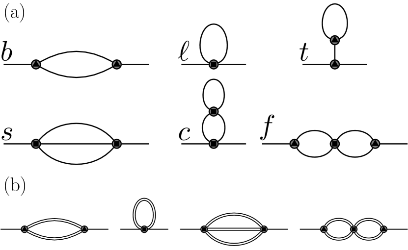
Figure 1: (a) A schematic of the $O(\lambda^{2})$ and $O(\lambda^{4})$ bare self-energy diagrams considered in this work; corresponding labels are provided. Vertices are bare cubic or quartic phonon interactions, while lines are the non-interacting phonon Green’s functions. (b) A schematic of the dressed self-energy diagrams evaluated in this work. Vertices are bare cubic or quartic phonon interactions, while lines are self-consistent phonon Green’s functions obtained using the Hartree-Fock or quasiparticle approach.

Including higher order diagrams beyond $O(\lambda^{4})$ is cumbersome, and a more convenient approach is to perform a self-consistent perturbation theory in terms of the dressed Green’s function and skeleton diagrams [68]. Perhaps the simplest approach is the previously discussed Hartree-Fock approximation for phonons. In the case where symmetry fixes the expectation values of the nuclear positions, the Hartree-Fock approximation is simply a self-consistent solution of the Dyson equation using the $\ell$ diagram. In this case, an infinite number of bare diagrams would be summed, including the $c$ diagram, though an infinite number of diagrams are still neglected, such as $s$ or any diagram containing a cubic vertex. The result of this approach is a real, frequency independent self-energy which renormalizes the bare phonon frequencies, though it does not produce a finite linewidth.

One approach for going beyond Hartree-Fock is to use the resulting self-consistent Hartree-Fock Green’s function to evaluate the $b$ diagram, which is known as the improved self-consistent (ISC) method [69], and the ISC is executed in the present work. The ISC based upon the SCP has been used in realistic computations of temperature dependent phonon spectrum [32, 31], soft-mode driven phase transitions [29, 35], thermal expansion [34, 33], and thermal conductivity [28]. An approach which goes beyond the ISC is the time-dependent self-consistent harmonic approximation (TD-SCHA) [70, 71], which constructs the Green’s function purely from quantities that are stochastically measured within Hartree-Fock. Recent applications of TD-SCHA within the bubble approximation [70], which is comparable to ISC, have produced reasonable predictions for the Raman and infrared spectra in ice [72] and hydrogen under large pressures [47], in addition to providing a reasonable description of the inelastic x-ray scattering function in NaCl and KCl at room temperature [73]. While the TD-SCHA goes beyond the ISC, it is still a somewhat limited theory given that important diagrams are neglected. For example, the TD-SCHA will not capture the effects of the sunset diagram, which is known to be critical even at room temperature in select systems [64, 65, 66], and we will demonstrate that it is important in CaF₂ beyond $T=500$ K.

An obvious approach for further potential improvement would be to use the Hartree-Fock Green’s function to evaluate both the $b$ and $s$ diagrams, which we execute in this study (see Figure S1 in Supplemental Material for a schematic [74]). A final approach is to use quasiparticle perturbation theory [75, 76] and include the real contribution of $b$ in the self-consistency and then use the resulting Green’s function to evaluate $s$, which we also execute. We are not aware of any previous quasiparticle perturbation theory calculations for phonons which include frequency dependent diagrams, though very recently a “one-shot” approximation was performed [29]. A downside of quasiparticle perturbation theory is that it is not a conserving approximation [77].

In this study we focus on the prototypical fluorite crystal CaF₂, where we previously computed quadratic and cubic irreducible derivatives using DFT with the strongly constrained and appropriately normed functional [78]. We demonstrated that the linewidth of the inelastic neutron scattering function computed using the $b$ diagram was in good agreement with experiment throughout the Brillouin zone at room temperature. This stringent test validated the quality of our quadratic and cubic irreducible derivatives, and therefore the underlying density functional which was used to compute them, in addition to the exclusive use of the $b$ diagram to compute the Green’s function. In the present work, we extend the Taylor series to include quartic interactions, and our goal is scrutinize a hierarchy of approximations which are used to compute the real and imaginary part of the phonon self-energy.

II Methodology

The vibrational Hamiltonian for CaF₂ is computed from density functional theory using the lone and bundled irreducible derivative approaches (see Section III for details). Here we outline how to compute the phonon self-energy [59], $\Sigma_{\boldsymbol{q}jj^{\prime}}(\omega)=\Delta_{\boldsymbol{q}jj^{\prime}}(\omega)-\textrm{i}\Gamma_{\boldsymbol{q}jj^{\prime}}(\omega)$, in various approximations, which can be used to construct the phonon lineshifts and linewidths. The contribution of a given self-energy diagram is denoted $\Sigma_{\boldsymbol{q}jj^{\prime}}^{A,a}$, where $a\in\{b,\ell,s,t,c,f\}$ labels a given diagram (see Fig. 1) and $A\in\{o,HF,QP\}$ labels which Green’s function was used to evaluate the diagram; where $o$, $HF$, and $QP$ correspond to the bare, Hartree-Fock, and quasiparticle Green’s function. The $HF$ and $QP$ Green’s functions are obtained by self-consistently solving for the roots of $|\omega^{2}-\boldsymbol{V}_{\boldsymbol{q}}(\omega)|$, where

$$V_{\boldsymbol{q}jj^{\prime}}(\omega) =(\omega^{0}_{\boldsymbol{q}j})^{2}\delta_{jj^{\prime}}+\left(2\omega_{\boldsymbol{q}j}\right)^{\frac{1}{2}}\left(2\omega_{\boldsymbol{q}j^{\prime}}\right)^{\frac{1}{2}}\Delta_{\boldsymbol{q}jj^{\prime}}(\omega),$$ (1)

$\omega^{0}_{\boldsymbol{q}j}$ is the bare phonon frequency, and $\omega_{\boldsymbol{q}j}$ is the renormalized phonon frequency. In the case of $HF$, the functional form of $\Delta_{\boldsymbol{q}jj^{\prime}}$ is given by the $\ell$ diagram, while for $QP$ the form of $\Delta_{\boldsymbol{q}jj^{\prime}}$ is given by the combination of the $\ell$ diagram and the real part of the $b$ diagram. The zeros of Eq. 1 deliver the updated renormalized frequencies and corresponding eigenvectors, which are then used to evaluate the updated $\Delta_{\boldsymbol{q}jj^{\prime}}$, and the process is iterated until self-consistency is achieved. The resulting self-consistent $\Delta_{\boldsymbol{q}jj^{\prime}}$ is then used to construct the $HF$ or $QP$ Green’s function. For the $QP$ case, we also test a “one-shot” approximation, as recently implemented in Ref. [29], which replaces the $QP$ self-consistency condition and instead uses $\Delta^{HF,\ell}_{jj^{\prime}}+\Delta^{HF,b}_{jj^{\prime}}$ to construct the $QP$ Green’s function.

For a given scheme $A$, the self-energy is then approximated $\Sigma_{\boldsymbol{q}jj^{\prime}}(\omega)\approx\sum_{a}\Sigma_{\boldsymbol{q}jj^{\prime}}^{A,a}(\omega)$. Given that the contribution from each diagram is additive, it can be useful to analyze results for various combinations of diagrams. Therefore, we introduce a notation to indicate which scheme and diagrams are used to construct a given result as $\mathcal{S}^{A}_{ijk\dots}$, where $A$ labels the scheme and $i,j,k,\dots$ indicate all diagrams evaluated. In this notation, the ISC approach [69] is denoted $\mathcal{S}^{HF}_{\ell b}$, and the recent one-shot quasiparticle calculation in Ref. [29] is an approximation to $\mathcal{S}^{QP}_{\ell b}$. In this paper, the most diagrams evaluated in each scheme are $\mathcal{S}^{o}_{\ell bsfc}$, $\mathcal{S}^{HF}_{\ell bsf}$, and $\mathcal{S}^{QP}_{\ell bsf}$. All of the diagrammatic approaches in this study are fully quantum mechanical approaches, but we evaluate them in the classical limit by replacing the Bose-Einstein distribution with $n(\omega)\rightarrow k_{B}T/\hbar\omega$ and neglecting the zero-point contribution.

Standard molecular dynamics approaches can be used to obtain the classical solution of the anharmonic Hamiltonian constructed from irreducible derivatives, which we refer to as irreducible derivative molecular dynamics (IDMD). Using the IDMD trajectory, the classical phonon spectral energy density $\mathcal{D}(\mathbf{q},\omega)$ at reciprocal point $\mathbf{q}$ is computed as

$$\mathcal{D}(\mathbf{q},\omega) =\frac{1}{2\pi N}\sum_{\mathbf{l}\mathbf{l}^{\prime}}e^{-i\mathbf{q}\cdot(\mathbf{l}-\mathbf{l^{\prime}})}$$

$$\times\sum_{dd^{\prime}}\int d\tau e^{-i\omega\tau}\left<\mathbf{r}(\mathbf{l}d,\tau)\cdot\mathbf{r}(\mathbf{l}^{\prime}d^{\prime},0)\right>,$$ (2)

where $\mathbf{l}$ labels the lattice translation, $d$ labels atoms within the primitive unit cell, $\mathbf{r}(\mathbf{l}d)$ is the displacement associated with translation $\mathbf{l}$ and basis atom $d$, and $N$ is the number of unit cells in the crystal. The quantum $\mathcal{D}(\mathbf{q},\omega)$ can be constructed from the quantum single particle phonon Green’s function $D_{\boldsymbol{q}j}(\omega)$ as [59, 79]

$$\mathcal{D}(\mathbf{q},\omega)=-\frac{\hbar n(\omega)}{2\pi}\sum_{j}\frac{\imaginary(D_{\boldsymbol{q}j}(\omega))}{\omega_{\boldsymbol{q}j}^{0}}\sum_{dd^{\prime}}\frac{\mathbf{e}_{\mathbf{q}jd}\cdot\mathbf{e}_{-\mathbf{q}jd^{\prime}}}{\sqrt{M_{d}M_{d^{\prime}}}},$$ (3)

where $M$ is the mass of the nuclei, $n(\omega)$ is the Bose-Einstein distribution, and $\mathbf{e}_{\mathbf{q}jd}$ is the polarization of atom $d$ in the mode $j$. The imaginary part of $D(\mathbf{q},\omega)$ can be written in terms of the self-energy as [59]

$$\imaginary(D_{\boldsymbol{q}j}(\omega)))=$$

$$\frac{-4\big{(}\omega_{\boldsymbol{q}j}^{0}\big{)}^{2}\Gamma_{\boldsymbol{q}jj}(\omega)}{\big{(}\omega^{2}-(\omega_{\boldsymbol{q}j}^{0})^{2}-2\omega_{\boldsymbol{q}j}^{0}\Delta_{\boldsymbol{q}jj}(\omega)\big{)}^{2}+\big{(}2\Gamma_{\boldsymbol{q}jj}(\omega)\omega_{\boldsymbol{q}j}^{0}\big{)}^{2}}.$$ (4)

Equations 3 and 4 can be applied in the classical limit, allowing one to relate the numerical measurements in Eq. 2 to the classical limit of the self-energy. The simplest quasiparticle interpretation of some peak in $\mathcal{D}(\boldsymbol{q},\omega)$ which is identified with $\omega_{\boldsymbol{q}j}^{0}$ can be characterized by the following trial function

$$C_{0}\frac{4\big{(}\omega_{\boldsymbol{q}j}^{0}\big{)}^{2}C_{2}}{\big{(}\omega^{2}-(\omega_{\boldsymbol{q}j}^{0})^{2}-2\omega_{\boldsymbol{q}j}^{0}C_{1}\big{)}^{2}+\big{(}2C_{2}\omega_{\boldsymbol{q}j}^{0}\big{)}^{2}},$$ (5)

which has three unknown coefficients $C_{0}$, $C_{1}$, and $C_{2}$. For a given $\omega_{\boldsymbol{q}j}^{0}$, the corresponding peak in the IDMD measured $\mathcal{D}(\boldsymbol{q},\omega)$ will be used to fit the three unknowns using linear regression. The energy window used to determine which data are included in the fit is 5 times the linewidth obtained from $\mathcal{S}^{o}_{\ell bs}$. In cases of overlapping peaks in $\mathcal{D}(\boldsymbol{q},\omega)$, the corresponding peaks are individually resolved in the basis of the unperturbed eigenmodes and associated with the corresponding $\omega_{\boldsymbol{q}j}^{0}$. The parameters resulting from the fitting process may be interpreted as the phonon lineshift $\Delta_{\boldsymbol{q}jj}(\omega_{\boldsymbol{q}j}^{0})=C_{1}$ and half linewidth $\Gamma_{\boldsymbol{q}jj}(\omega_{\boldsymbol{q}j}^{0})=C_{2}$.

III Computational Details

DFT calculations within the local density approximation (LDA)[80] were performed using the projector augmented wave (PAW) method [67, 81], as implemented in the Vienna ab initio simulation package (VASP) [82, 83, 84, 85]. A plane wave basis with an energy cutoff of 600 eV was employed, along with a $k$-point density consistent with a centered k-point mesh of 20$\times$20$\times$20 in the primitive unit cell. All k-point integrations were done using the tetrahedron method with Blöchl corrections [67]. The DFT energies were converged to within $10^{-6}$ eV, while ionic relaxations were converged to within $10^{-5}$ eV. The structure was relaxed yielding a lattice parameter of 5.330 Å, in agreement with previous work [86]. The lattice constant is fixed in all calculations, and we do not consider thermal expansion in the present work, though it is straightforward to incorporate the strain dependence of the irreducible derivatives [87]. The face-centered cubic lattice vectors are encoded in a $3\times 3$ row stacked matrix $\hat{\mathbf{a}}=\frac{a_{o}}{2}(\hat{\mathbf{J}}-\hat{\mathbf{1}})$, where $\hat{\mathbf{1}}$ is the identity matrix and $\hat{\mathbf{J}}$ is a matrix in which each element is 1. The quartic irreducible derivatives were calculated via the bundled irreducible derivative (BID) approach [8], and the quadratic and cubic terms were computed in previous work [78]. Up to 10 finite difference discretizations were evaluated for a given measurement, such that robust error tails could be constructed and used to extrapolate to zero discretization. While the BID method only requires the absolute minimum number of measurements as dictated by group theory, we tripled this minimum number in order to reduce the possibility of contamination due to a defective measurement. The LO-TO splitting was treated using the standard dipole-dipole approach [88, 89] and implemented using irreducible derivatives [87].

The Brillouin zone is discretized using a real space supercell $\hat{\mathbf{S}}_{BZ}\hat{\mathbf{a}}$, where $\hat{\mathbf{S}}_{BZ}$ is an invertible matrix of integers which produces superlattice vectors that satisfy the point group [8]. Two classes of supercells are used: $n\hat{\mathbf{1}}$ and $n\hat{\mathbf{S}}_{O}=n(4\hat{\mathbf{1}}-\hat{\mathbf{J}})$; where $n$ is a positive integer. The second, third, and fourth order irreducible derivatives were computed for $\hat{\mathbf{S}}_{BZ}=4\hat{\mathbf{1}}$ (containing 64 primitive cells), $\hat{\mathbf{S}}_{BZ}=\hat{\mathbf{S}}_{O}$ (containing 16 primitive cells), and $2\hat{\mathbf{1}}$, respectively. The quadratic and cubic irreducible derivatives have been previously computed and reported [78], and the quartic terms are reported in Supplemental Material [74]. A plot of the computed phonon band structure, including branch labels, is shown in Figure 2.

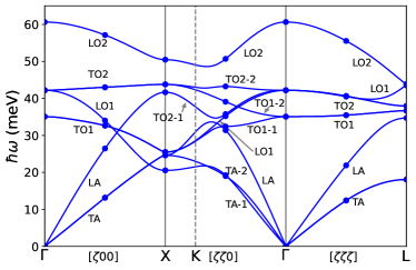
Figure 2: The phonon dispersion of CaF₂, including branch labels. Points are computed from DFT and lines are a Fourier interpolation.

The IDMD method is implemented using an interface to the LAMMPS [90, 91] software package. The irreducible derivatives are Fourier interpolated to a $10\times 10\times 10$ supercell. The Nose-Hoover thermostat [92] is used along with a 1 fs time step. For a given trajectory at each temperature, 30,000 steps are performed for initialization followed by 600,000 steps. Five trajectories are performed at each temperature, and all observables are averaged over the five trajectories. For all diagrammatic calculations, including self-consistent calculations, irreducible derivatives are Fourier interpolated to a $10\times 10\times 10$ supercell, and all integrations over the Brillouin Zone involving the Dirac delta function are performed using the tetrahedron method [67]. The real part of the self-energy was obtained via a Kramers-Kronig transformation of the imaginary part.

IV Results and Discussion

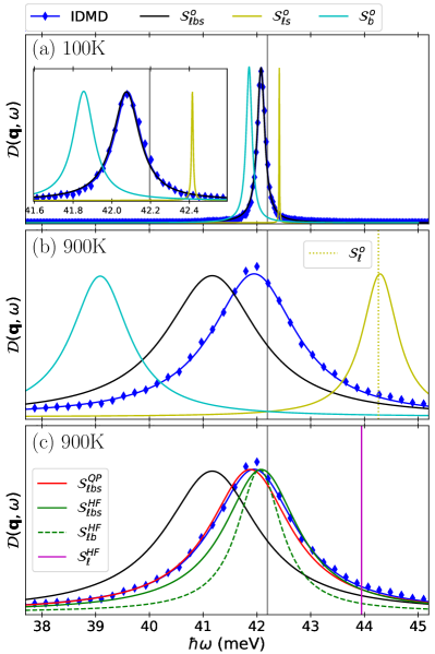
Figure 3: Plots of $\mathcal{D}(\mathbf{q},\omega)$ at the $\Gamma$ point for an energy window around the T_2g modes. The IDMD results are shown as blue diamonds, and the fit is shown as a blue curve. The harmonic phonon frequency is denoted as a gray vertical line. ($a$, $b$) Results at $T=100$ K and $T=900$ K for IDMD and bare perturbation theory for various diagrams. ($c$) Results at $T=900$ K for $\mathcal{S}^{QP}$, $\mathcal{S}^{HF}_{\ell bs}$, $\mathcal{S}^{HF}_{\ell b}$, and $\mathcal{S}^{HF}_{\ell}$, in addition to IDMD and $\mathcal{S}^{o}_{\ell bs}$ results. Results for $\mathcal{S}^{o}_{b}$ and $\mathcal{S}^{o}_{\ell s}$ at 100K were rescaled by 0.94 and 0.06, respectively. Results for $\mathcal{S}^{o}_{b}$, $\mathcal{S}^{o}_{\ell s}$, $\mathcal{S}^{o}_{\ell bs}$, and $\mathcal{S}^{HF}_{\ell bs}$ at 900K were rescaled by 0.70, 0.43, 1.13, 0.90, and 0.54, respectively.

We begin by examining $\mathcal{D}(\mathbf{q},\omega)$ at the $\Gamma$-point in an energy window around the T_2g modes (i.e. LO1 and TO2) to illustrate the various methods used to solve the vibrational Hamiltonian, which contains up to quartic terms. We will explore a low temperature and a high temperature, though a very extensive survey is provided in Supplemental Material [74]. We first consider the low temperature of $T=100$ K, where the classical perturbative approaches should be able to reasonably describe the IDMD (see Figure 3, panel $a$). The IDMD results are shown as blue diamonds, where each point is the result of binning all measurements within a 0.02 meV window, and the blue line is the result of fitting equation 5 to the raw spectrum. We begin by comparing $\mathcal{S}^{o}_{\ell bs}$ to the IDMD spectra (see inset), demonstrating excellent agreement with both the line shift and width, where the former is -0.12 meV and the latter is 0.16 meV. It is interesting to further decompose the result of $\mathcal{S}^{o}_{\ell bs}$ into $\mathcal{S}^{o}_{b}$ and $\mathcal{S}^{o}_{\ell s}$, demonstrating that $\mathcal{S}^{o}_{b}$ is almost entirely responsible for the linewidth, but it also substantially shifts the mode as well. However, the shift from $\mathcal{S}^{o}_{b}$ is partially cancelled by the shift from $\mathcal{S}^{o}_{\ell s}$, and it should be noted that the contribution from $\mathcal{S}^{o}_{s}$ is essentially negligible at this temperature. This compensation of the shift between $\mathcal{S}^{o}_{b}$ and $\mathcal{S}^{o}_{\ell}$ is not uncommon [61], and it helps justify the success of thermal conductivity calculations solely using the bare phonon frequencies and the $\mathcal{S}^{o}_{b}$ scattering mechanism when solving the linearized Boltzmann transport equation. The satisfactory performance of bare perturbation theory implies that there is no need to consider self-consistent perturbation theory at this temperature.

We now proceed to the much higher temperature of $T=900K$, where the shift and width are substantially larger (see Fig 3, panel $b$). As in the low temperature case, $\mathcal{S}^{o}_{b}$ causes a downward shift and generates a non-trivial linewidth. Unlike the low temperature case, $\mathcal{S}^{o}_{\ell s}$ not only shifts the peak upward, but also generates a substantial linewidth. Given that $\mathcal{S}^{o}_{\ell}$ is purely real, all of the linewidth contribution of $\mathcal{S}^{o}_{\ell s}$ arises from $\mathcal{S}^{o}_{s}$, demonstrating that $\mathcal{S}^{o}_{s}$ can be an important contribution to the imaginary part of the self-energy at higher temperatures. Taking all contributions together, the $\mathcal{S}^{o}_{\ell bs}$ provides a reasonable description of the IDMD result, though there is a clear error in the shift, which suggests that self-consistent perturbation theory may be needed. Indeed, $\mathcal{S}^{QP}_{\ell bs}$ provides an excellent description of the IDMD results (see Fig 3, panel $c$). When moving down one level to $\mathcal{S}^{HF}_{\ell bs}$, the only notable degradation of the result is a small shift to higher frequencies. It is also interesting to consider $\mathcal{S}^{HF}_{\ell b}$ (i.e. the ISC) which shows a substantial error in the linewidth. Furthermore, it is useful to consider the $f$ diagram, given that it is recovered by TD-SCHA, and we find that it only has a very small contribution to both the linewidth and lineshift when evaluating any of the aforementioned schemes [74].

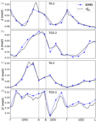
Figure 4: Phonon lineshifts ($a$, $b$) and linewidths ($c$, $d$) of the TA-2 ($a$, $c$) and TO2-2 ($b$, $d$) modes at $T=100$ K along various paths through the Brillouin zone. IDMD and $\mathcal{S}^{o}_{\ell bs}$ results are blue squares and black curves, respectively. Curves between data points are guides to the eye.

The preceding analysis carefully explored the results of different diagrams for a single mode, and we now proceed to survey select branches throughout the Brillouin zone. We begin by examining the phonon line shift and width of the TA-2 and TO2-2 modes at $T=100$ K (see Figure 4). For both the line shifts and widths, the $\mathcal{S}^{o}_{\ell bs}$ yields results that are close to the IDMD. There are some regions where small differences can be noted, and care must be taken when scrutinizing the results given the overall small magnitude of the numbers at hand. Nonetheless, the differences mostly appear to arise from higher order diagrams, given that including self-consistency mostly tends to move the diagrammatic solution closer to the IDMD (see Supplemental Material [74]). The results for the remaining modes are comparable [74].

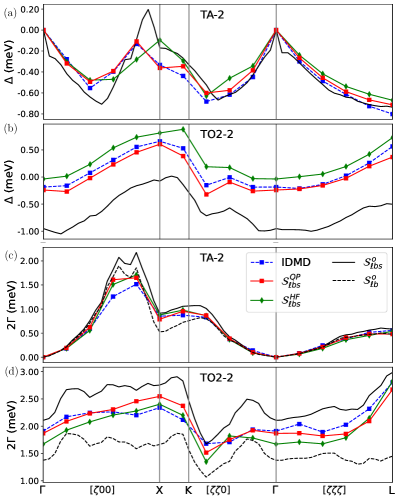
Figure 5: Phonon lineshifts ($a$, $b$) and linewidths ($c$, $d$) of the TA-2 ($a$, $c$) and TO2-2 ($b$, $d$) modes at $T=900$ K along various paths through the Brillouin zone. IDMD, $\mathcal{S}^{QP}_{\ell bs}$, $\mathcal{S}^{HF}_{\ell bs}$, $\mathcal{S}^{o}_{\ell bs}$, and $\mathcal{S}^{o}_{b}$ results are blue squares, red curves, green curves, black curves, and dashed black curves, respectively. Curves between data points are guides to the eye.

Having established the fidelity of our diagrammatic approaches and IDMD at low temperatures, we now proceed to the high temperature of $T=900$ K where IDMD can be used to judge the accuracy of different levels of bare and self-consistent perturbation theory (see Figure 5). As done previously, we explore the TA-2 and TO2-2 modes, but here we consider self-consistent perturbation theory as well given the deficiency of bare perturbation theory at this temperature. We begin by examining the shift of the TA-2 mode (panel $a$), where $\mathcal{S}^{o}_{\ell bs}$ yields good results in certain portions of the zone, but performs poorly in selected regions. Including self-consistency via $\mathcal{S}^{QP}_{\ell bs}$ and $\mathcal{S}^{HF}_{\ell bs}$ tends to correct large deviations that are observed in $\mathcal{S}^{o}_{\ell bs}$. For the shift of the TO2-2 modes (panel $b$), the $\mathcal{S}^{o}_{\ell bs}$ result yields a more systematic error, where the results are shifted in a nearly uniform manner, and the result even has the wrong sign in some cases. In this case, $\mathcal{S}^{HF}_{\ell bs}$ offers a drastic improvement, and $\mathcal{S}^{QP}_{\ell bs}$ pushes the result even closer to IDMD. The linewidths have similar behavior to the lineshifts in the two respective cases (see panels $c$ and $d$). In the case of TA-2, it is interesting to consider $\mathcal{S}^{o}_{b}$, given its importance in the context of common treatments of thermal conductivity, and it is clear that it yields remarkable results. However, $\mathcal{S}^{o}_{b}$ performs poorly for the TO2-2 modes. It is also interesting to consider the effect of the $f$ diagram, and it is shown to only have a small effect on both the linewidths and lineshifts [74]. The general trends that we have outlined here can also be seen in other modes, and comprehensive results for all branches at temperatures of 100K, 300K, 500K, 700K, and 900K are included in Supplemental Material [74]. We also provide a corresponding analysis where all cubic interactions are set to zero [74].

V Conclusion

In summary, we have computed the irreducible derivatives of CaF₂ up to fourth order, defining the vibrational Hamiltonian. We use molecular dynamics to solve the vibrational Hamiltonian, which we refer to as irreducible derivative molecular dynamics (IDMD), yielding the real and imaginary part of the phonon self-energy in the classical limit. The IDMD result was then used as a benchmark for various levels of diagrammatic perturbation theory. At the low temperature of $T=100$ K, we show that bare perturbation performs well using the $b$, $\ell$, and $s$ diagrams (i.e. $\mathcal{S}^{o}_{\ell bs}$). While the linewidth is reasonably well described by the $b$ diagram alone at $T=100$ K, the $\ell$ diagram is also necessary to properly capture the lineshift. At the high temperature of $T=900$ K, bare perturbation theory only performs well for the linewidths of the acoustic modes, where even the $b$ diagram alone yields reasonable results. Treating the $\ell$ diagram self-consistently and evaluating the $b$ and $s$ diagrams post self-consistency (i.e. $\mathcal{S}^{HF}_{\ell bs}$) is critical to obtaining accurate lineshifts for all branches, in addition to obtaining accurate linewidths for the optical modes. Further improvement is normally obtained when performing quasiparticle self-consistent perturbation theory, where the real part of the $b$ diagram is used during self-consistency (i.e. $\mathcal{S}^{QP}_{\ell bs}$). While we only executed self-consistent perturbation theory in the classical limit in this work, it should be emphasized that the quantum case has the same computational cost and poses no difficulty beyond the classical case.

The procedure outlined in this paper of assessing various levels of diagrammatic perturbation theory in the classical limit using molecular dynamics should be viable on nearly any system where the Taylor series can be constructed. Once some class of diagrams is validated classically, it is likely that the quantum counterparts will also perform well at lower temperatures in the quantum regime so long as the anharmonicity is sufficiently weak. Furthermore, the prescribed diagrams may be combined with other diagrammatic approaches to scattering, such as defects or electron-phonon coupling in the case of metals. An obvious application of the philosophy of this paper would be phonon mediated thermal conductivity, where the molecular dynamics solution would yield the thermal conductivity within Kubo-Green linear response, and various levels of self-consistent diagrammatic perturbation theory could be tested in conjunction with the linearized Boltzmann transport equation in the classical limit.

VI Acknowledgments

We are grateful to Zhengqian Cheng for fruitful discussions. This work was supported by the grant DE-SC0016507 funded by the U.S. Department of Energy, Office of Science. This research used resources of the National Energy Research Scientific Computing Center, a DOE Office of Science User Facility supported by the Office of Science of the U.S. Department of Energy under Contract No. DE-AC02-05CH11231.

References

- Wallace [1998] D. Wallace, Thermodynamics of Crystals (Dover, 1998).
- Wendel and Martin [1978] H. Wendel and R. M. Martin, Phys. Rev. Lett. 40, 950 (1978).
- Gonze [1995] X. Gonze, Physical Review A 52, 1096 (1995).
- Debernardi et al. [1995] A. Debernardi, S. Baroni, and E. Molinari, Phys. Rev. Lett. 75, 1819 (1995).
- Lindsay et al. [2019] L. Lindsay, A. Katre, A. Cepellotti, and N. Mingo, Journal Of Applied Physics 126, 050902 (2019).
- Vanderbilt et al. [1989] D. Vanderbilt, S. H. Taole, and S. Narasimhan, Phys. Rev. B 40, 5657 (1989).
- Narasimhan and Vanderbilt [1991] S. Narasimhan and D. Vanderbilt, Phys. Rev. B 43, 4541 (1991).
- Fu et al. [2019] L. Fu, M. Kornbluth, Z. Cheng, and C. A. Marianetti, Phys. Rev. B 100, 014303 (2019), publisher: American Physical Society.
- Ceperley [1995] D. M. Ceperley, Rev. Mod. Phys. 67, 279 (1995).
- Ceperley [1999] D. M. Ceperley, Rev. Mod. Phys. 71, 438 (1999).
- Ramirez et al. [2006] R. Ramirez, C. P. Herrero, and E. R. Hernandez, Phys. Rev. B 73, 245202 (2006).
- Ramirez et al. [2008] R. Ramirez, C. P. Herrero, E. R. Hernandez, and M. Cardona, Phys. Rev. B 77, 045210 (2008).
- Jarrell and Gubernatis [1996] M. Jarrell and J. E. Gubernatis, Physics Reports-review Section Of Physics Letters 269, 133 (1996).
- Sorkin et al. [2005] V. Sorkin, E. Polturak, and J. Adler, Phys. Rev. B 71, 214304 (2005).
- Perez et al. [2009] A. Perez, M. E. Tuckerman, and M. H. Muser, Journal Of Chemical Physics 130, 184105 (2009).
- Althorpe [2021] S. C. Althorpe, European Physical Journal B 94, 155 (2021).
- Habershon et al. [2013] S. Habershon, D. E. Manolopoulos, T. E. Markland, and T. F. Miller, Annual Review Of Physical Chemistry, Vol 64 Se Annual Review Of Physical Chemistry 64, 387 (2013).
- Luo and Yu [2020] R. P. Luo and K. Yu, Journal Of Chemical Physics 153, 194105 (2020).
- Wang et al. [1990] C. Z. Wang, C. T. Chan, and K. M. Ho, Phys. Rev. B 42, 11276 (1990), publisher: American Physical Society.
- Glensk et al. [2019] A. Glensk, B. Grabowski, T. Hickel, J. Neugebauer, J. Neuhaus, K. Hradil, W. Petry, and M. Leitner, Phys. Rev. Lett. 123, 235501 (2019).
- Esfarjani et al. [2011] K. Esfarjani, G. Chen, and H. T. Stokes, Phys. Rev. B 84, 085204 (2011).
- Shiomi et al. [2011] J. Shiomi, K. Esfarjani, and G. Chen, Phys. Rev. B 84, 104302 (2011), publisher: American Physical Society.
- Murakami et al. [2013] T. Murakami, T. Shiga, T. Hori, K. Esfarjani, and J. Shiomi, EPL 102, 46002 (2013), publisher: IOP Publishing.
- Shiga et al. [2014] T. Shiga, T. Murakami, T. Hori, O. Delaire, and J. Shiomi, Appl. Phys. Express 7, 041801 (2014), publisher: IOP Publishing.
- Zhou et al. [2019] F. Zhou, W. Nielson, Y. Xia, and V. Ozoliņš, Phys. Rev. B 100, 184308 (2019).
- Hooton [1955] D. Hooton, The London, Edinburgh, and Dublin Philosophical Magazine and Journal of Science 46, 422 (1955), publisher: Taylor & Francis _eprint: https://doi.org/10.1080/14786440408520575.
- Jones and March [2011] W. Jones and N. H. March, Theoretical Solid State Physics, Volume 1: Perfect Lattices in Equilibrium (Dover Publications, New York, 2011).
- Tadano and Tsuneyuki [2018a] T. Tadano and S. Tsuneyuki, Phys. Rev. Lett. 120, 105901 (2018a), publisher: American Physical Society.
- Tadano and Saidi [2022] T. Tadano and W. A. Saidi, Phys. Rev. Lett. 129, 185901 (2022).
- Zhou et al. [2014] F. Zhou, W. Nielson, Y. Xia, and V. Ozolins, Physical Review Letters 113, 185501 (2014), publisher: American Physical Society.
- Tadano and Tsuneyuki [2018b] T. Tadano and S. Tsuneyuki, Journal of the Physical Society of Japan 87, 041015 (2018b), arXiv: 1706.04744.
- Tadano and Tsuneyuki [2015] T. Tadano and S. Tsuneyuki, Phys. Rev. B 92, 054301 (2015), publisher: American Physical Society.
- Masuki et al. [2022a] R. Masuki, T. Nomoto, R. Arita, and T. Tadano, Physical Review B 105, 064112 (2022a), publisher: American Physical Society.
- Oba et al. [2019] Y. Oba, T. Tadano, R. Akashi, and S. Tsuneyuki, Phys. Rev. Materials 3, 033601 (2019), publisher: American Physical Society.
- Masuki et al. [2022b] R. Masuki, T. Nomoto, R. Arita, and T. Tadano, Physical Review B 106, 224104 (2022b), publisher: American Physical Society.
- Errea et al. [2014] I. Errea, M. Calandra, and F. Mauri, Physical Review B 89, 064302 (2014), publisher: American Physical Society.
- Bianco et al. [2017] R. Bianco, I. Errea, L. Paulatto, M. Calandra, and F. Mauri, Phys. Rev. B 96, 014111 (2017), publisher: American Physical Society.
- Errea et al. [2011] I. Errea, B. Rousseau, and A. Bergara, Phys. Rev. Lett. 106, 165501 (2011), publisher: American Physical Society.
- Leroux et al. [2015] M. Leroux, I. Errea, M. Le Tacon, S.-M. Souliou, G. Garbarino, L. Cario, A. Bosak, F. Mauri, M. Calandra, and P. Rodiere, Physical Review B 92, 140303(R) (2015), publisher: American Physical Society.
- Errea et al. [2013] I. Errea, M. Calandra, and F. Mauri, Phys. Rev. Lett. 111, 177002 (2013), publisher: American Physical Society.
- Errea et al. [2015] I. Errea, M. Calandra, C. J. Pickard, J. Nelson, R. J. Needs, Y. Li, H. Liu, Y. Zhang, Y. Ma, and F. Mauri, Phys. Rev. Lett. 114, 157004 (2015), publisher: American Physical Society.
- Errea et al. [2016] I. Errea, M. Calandra, C. J. Pickard, J. R. Nelson, R. J. Needs, Y. Li, H. Liu, Y. Zhang, Y. Ma, and F. Mauri, Nature 532, 81 (2016), number: 7597 Publisher: Nature Publishing Group.
- Borinaga et al. [2016a] M. Borinaga, I. Errea, M. Calandra, F. Mauri, and A. Bergara, Physical Review B 93, 174308 (2016a), publisher: American Physical Society.
- Borinaga et al. [2016b] M. Borinaga, P. Riego, A. Leonardo, M. Calandra, F. Mauri, A. Bergara, and I. Errea, Journal of Physics: Condensed Matter 28, 494001 (2016b), publisher: IOP Publishing.
- Bianco et al. [2018] R. Bianco, I. Errea, M. Calandra, and F. Mauri, Phys. Rev. B 97, 214101 (2018), publisher: American Physical Society.
- Errea et al. [2020] I. Errea, F. Belli, L. Monacelli, A. Sanna, T. Koretsune, T. Tadano, R. Bianco, M. Calandra, R. Arita, F. Mauri, and J. A. Flores-Livas, Nature 578, 66 (2020), number: 7793 Publisher: Nature Publishing Group.
- Monacelli et al. [2021] L. Monacelli, I. Errea, M. Calandra, and F. Mauri, Nature Physics 17, 63 (2021), number: 1 Publisher: Nature Publishing Group.
- Souvatzis et al. [2008] P. Souvatzis, O. Eriksson, M. I. Katsnelson, and S. P. Rudin, Physical Review Letters 100, 095901 (2008), publisher: American Physical Society.
- Souvatzis et al. [2009] P. Souvatzis, O. Eriksson, M. I. Katsnelson, and S. P. Rudin, Computational Materials Science 44, 888 (2009).
- Lazar et al. [2011] P. Lazar, M. Jahnatek, J. Hafner, N. Nagasako, R. Asahi, C. Blaas-Schenner, M. Stohr, and R. Podloucky, Physical Review B 84, 054202 (2011), publisher: American Physical Society.
- Soderlind et al. [2012] P. Soderlind, B. Grabowski, L. Yang, A. Landa, T. Bjorkman, P. Souvatzis, and O. Eriksson, Physical Review B 85, 060301(R) (2012), publisher: American Physical Society.
- Di Gennaro et al. [2013] M. Di Gennaro, S. K. Saha, and M. J. Verstraete, Physical Review Letters 111, 025503 (2013), publisher: American Physical Society.
- van Roekeghem et al. [2016] A. van Roekeghem, J. Carrete, and N. Mingo, Physical Review B 94, 020303(R) (2016), publisher: American Physical Society.
- van Roekeghem et al. [2021] A. van Roekeghem, J. Carrete, and N. Mingo, Computer Physics Communications 263, 107945 (2021).
- Hellman et al. [2011] O. Hellman, I. A. Abrikosov, and S. I. Simak, Physical Review B 84, 180301(R) (2011), publisher: American Physical Society.
- Hellman et al. [2013] O. Hellman, P. Steneteg, I. A. Abrikosov, and S. I. Simak, Physical Review B 87, 104111 (2013), publisher: American Physical Society.
- Heine et al. [2022] M. Heine, O. Hellman, and D. Broido, Physical Review Materials 6, 113805 (2022), publisher: American Physical Society.
- Kokkedee [1962] J. J. Kokkedee, Physica 28, 374 (1962).
- Maradudin and Fein [1962] A. A. Maradudin and A. E. Fein, Phys. Rev. 128, 2589 (1962).
- Tripathi and Pathak [1974] R. S. Tripathi and K. N. Pathak, Nuov Cim B 21, 289 (1974).
- Lazzeri et al. [2003] M. Lazzeri, M. Calandra, and F. Mauri, Phys. Rev. B 68, 220509(R) (2003).
- Broido et al. [2007] D. A. Broido, M. Malorny, G. Birner, N. Mingo, and D. A. Stewart, Appl. Phys. Lett. 91, 231922 (2007), publisher: American Institute of Physics.
- Lindsay et al. [2018] L. Lindsay, C. Hua, X. L. Ruan, and S. Lee, Materials Today Physics 7, 106 (2018).
- Kang et al. [2018] J. S. Kang, M. Li, H. A. Wu, H. Nguyen, and Y. J. Hu, Science 361, 575 (2018).
- Tian et al. [2018] F. Tian, B. Song, X. Chen, N. K. Ravichandran, Y. C. Lv, K. Chen, S. Sullivan, J. Kim, Y. Y. Zhou, T. H. Liu, M. Goni, Z. W. Ding, J. Y. Sun, G. Gamage, H. R. Sun, H. Ziyaee, S. Y. Huyan, L. Z. Deng, J. S. Zhou, A. J. Schmidt, S. Chen, C. W. Chu, P. Huang, D. Broido, L. Shi, G. Chen, and Z. F. Ren, Science 361, 582 (2018).
- Li et al. [2018] S. Li, Q. Y. Zheng, Y. C. Lv, X. Y. Liu, X. Q. Wang, P. Huang, D. G. Cahill, and B. Lv, Science 361, 579 (2018).
- Blochl et al. [1994] P. E. Blochl, O. Jepsen, and O. K. Andersen, Phys. Rev. B 49, 16223 (1994).
- Martin et al. [2016] R. M. Martin, L. Reining, and D. M. Ceperley, Interacting Electrons: Theory and Computational Approaches, 1st ed. (Cambridge University Press, 2016).
- Goldman et al. [1968] V. V. Goldman, G. K. Horton, and M. L. Klein, Phys. Rev. Lett. 21, 1527 (1968), publisher: American Physical Society.
- Monacelli and Mauri [2021] L. Monacelli and F. Mauri, Phys. Rev. B 103, 104305 (2021).
- Lihm and Park [2021] J.-M. Lihm and C.-H. Park, Physical Review Research 3, L032017 (2021), publisher: American Physical Society.
- Cherubini et al. [2021] M. Cherubini, L. Monacelli, and F. Mauri, The Journal of Chemical Physics 155, 184502 (2021), publisher: American Institute of Physics.
- Togo et al. [2022] A. Togo, H. Hayashi, T. Tadano, S. Tsutsui, and I. Tanaka, Journal of Physics: Condensed Matter 34, 365401 (2022), publisher: IOP Publishing.
- [74] See Supplemental Material at [URL will be inserted by publisher] for phonon lineshifts and linewidths for all branches from 100K to 900K, decomposition of , and irreducible derivatives.
- Faleev et al. [2004] S. V. Faleev, M. van Schilfgaarde, and T. Kotani, Phys. Rev. Lett. 93, 126406 (2004).
- van Schilfgaarde et al. [2006] M. van Schilfgaarde, T. Kotani, and S. Faleev, Phys. Rev. Lett. 96, 226402 (2006).
- Kutepov et al. [2012] A. Kutepov, K. Haule, S. Y. Savrasov, and G. Kotliar, Physical Review B 85, 155129 (2012), publisher: American Physical Society.
- Xiao et al. [2022] E. Xiao, H. Ma, M. S. Bryan, L. Fu, J. M. Mann, B. Winn, D. L. Abernathy, R. P. Hermann, A. R. Khanolkar, C. A. Dennett, D. H. Hurley, M. E. Manley, and C. A. Marianetti, Phys. Rev. B 106, 144310 (2022).
- Squires [2012] G. L. Squires, Introduction to the Theory of Thermal Neutron Scattering, 3rd ed. (Cambridge University Press, 2012).
- Perdew and Zunger [1981] J. P. Perdew and A. Zunger, Phys. Rev. B 23, 5048 (1981).
- Kresse and Joubert [1999] G. Kresse and D. Joubert, Phys. Rev. B 59, 1758 (1999).
- Kresse and Hafner [1993] G. Kresse and J. Hafner, Phys. Rev. B 47, 558 (1993).
- Kresse and Hafner [1994] G. Kresse and J. Hafner, Phys. Rev. B 49, 14251 (1994).
- Kresse and Furthmuller [1996a] G. Kresse and J. Furthmuller, Computational Materials Science 6, 15 (1996a).
- Kresse and Furthmuller [1996b] G. Kresse and J. Furthmuller, Phys. Rev. B 54, 11169 (1996b).
- Schmalzl et al. [2003] K. Schmalzl, D. Strauch, H. Schober, B. Dorner, and A. Ivanov, in High Performance Computing in Science and Engineering, Munich 2002, edited by S. Wagner, A. Bode, W. Hanke, and F. Durst (Springer Berlin Heidelberg, Berlin, Heidelberg, 2003) pp. 249–258.
- Mathis et al. [2022] M. A. Mathis, A. Khanolkar, L. Fu, M. S. Bryan, C. A. Dennett, K. Rickert, J. M. Mann, B. Winn, D. L. Abernathy, M. E. Manley, D. H. Hurley, and C. A. Marianetti, Phys. Rev. B 106, 014314 (2022).
- Gonze and Lee [1997] X. Gonze and C. Lee, Phys. Rev. B 55, 10355 (1997).
- Giannozzi et al. [1991] P. Giannozzi, S. deGironcoli, P. Pavone, and S. Baroni, Phys. Rev. B 43, 7231 (1991).
- Thompson et al. [2022] A. P. Thompson, H. M. Aktulga, R. Berger, D. S. Bolintineanu, W. M. Brown, P. S. Crozier, P. J. in ’t Veld, A. Kohlmeyer, S. G. Moore, T. D. Nguyen, R. Shan, M. J. Stevens, J. Tranchida, C. Trott, and S. J. Plimpton, Comp. Phys. Comm. 271, 108171 (2022).
- Plimpton [1995] S. Plimpton, Journal of Computational Physics 117, 1 (1995).
- Nosé [1984] S. Nosé, J. Chem. Phys. 81, 511 (1984), publisher: American Institute of Physics.