Analysis of V2X Sidelink Positioning in sub-6 GHz

Abstract

Radio positioning is an important part of joint communication and sensing in beyond 5G communication systems. Existing works mainly focus on the mmWave bands and under-utilize the sub-6 GHz bands, even though it is promising for accurate positioning, especially when the multipath is uncomplicated, and meaningful in several important use cases. In this paper, we analyze V2X sidelink positioning and propose a new performance bound that can predict the positioning performance in the presence of severe multipath. Simulation results using ray-tracing data demonstrate the possibility of sidelink positioning, and the efficacy of the new performance bound and its relation with the complexity of the multipath.

I Introduction

Sensing and positioning have gained significant attention in the evolution of 5G mobile radio systems [1]. Much of this attention has been devoted to the mmWave bands (both lower mmWave around 28 GHz and upper mmWave around 140 GHz), due to larger available bandwidth and commensurate distance resolution [2, 3]. Nevertheless, sub-6 GHz bands hold significant promise for accurate positioning as well, especially in scenarios without too complicated multipath. Due to the presence of the ITS 5850-5925 MHz band and the neighboring unlicensed bands, sub-6 GHz positioning over sidelinks has recently come into focus, complementary to enhancements for improved integrity, accuracy, and power efficiency [4]. Sidelink positioning is expected to be an important enabler for several use cases, considering positioning for the user equipments in in-coverage, partial coverage, and out-of-coverage. These include vehicle-to-anything (V2X), Internet of Things (IoT) (e.g., in private networks at 3.6–3.7 GHz), and public safety (e.g., first responders) [5].

Within V2X, there have been a number of studies related to sidelink positioning at sub-6 GHz. In terms of overviews, there are several recent papers [6, 7, 8, 9, 10, 11]. In [6], a broad overview of V2X positioning is provided, highlighting the limitations of time-difference-of-arrival (TDoA) in terms of synchronization, and proposes to use carrier phase and multipath information. In [7], use cases and corresponding requirements are specified, showing that beyond 5G systems need enhancements in terms of deployments, methods, and architectures. In [8], sidelink positioning is advocated as a positioning enabler with lower latency, higher line-of-sight (LoS) probability, and improved coverage, which should be able to operate both collaboratively with the network and to operate independently when the network is unavailable. Focusing on indoor IoT scenarios, [9] studies combinations of different measurements together with an extended Kalman filter (EKF). The relative merits of cellular vehicle-to-anything (C-V2X) and WiFi-based positioning are discussed and evaluated in [10], based on the WINNER+ model, indicating a preference of C-V2X. In [11], different positioning systems/architectures are described for vehicular positioning applications, along with relevant key performance indicators. There have also been several studies focusing exclusively on the physical layer [12, 13, 14, 15].

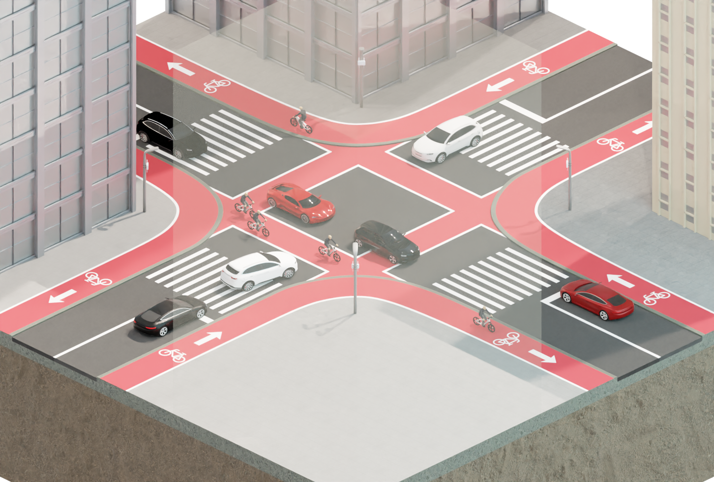
Figure 1: Illustration of an urban traffic situation involving vulnerable road users, vehicles, and road-side units.

Among these, [12] evaluates vehicle-to-infrastructure (V2I) ranging and TDoA positioning for LTE under different statistical channel models. In [13], dedicated short-range communications (DSRC) positioning is studied with ray-tracing data, combining angle-of-arrival (AoA) information at road-side units and vehicle-to-vehicle (V2V) cooperating ranging links. The use of several arrays per UE is proposed in [14] and evaluated in terms of Cramér-Rao bound (CRB) at 3.5 and 28 GHz, based on AoA and TDoA measurements. In [15], sensing with 5G-V2X waveforms is considered, determining the range and Doppler of passive targets via CRB analysis under a pure geometric channel, subject to interference. Finally, there are studies that focus mainly on algorithmic aspects, such as [16, 17, 18]. Here, [16] proposes a method for V2X localization with a single RSU from range measurements over time. In [17], V2V range and angle and V2I TDoA measurements are combined to improve positioning. In [18], a dynamic method is proposed to switch between global navigation satellite system (GNSS) and NR V2X TDoA measurements. While the above listed papers adopt widely varying assumption, models, methods, and evaluation methodologies, it is worth pointing out that [4] has proposed a common evaluation methodology and a set of common assumptions.

In this paper, we perform a realistic evaluation of sidelink V2X round-trip-time (RTT) positioning towards 3GPP Release 18 using ray-tracing data, focusing on operation outside of the network coverage.

• Use cases: We describe the relevant V2X use cases towards 3GPP Release 18 and requirements that involve sidelink positioning, as well as the related physical models, and limitations thereof.

• Novel performance bound: We propose a novel methodology based on Fisher information analysis to predict positioning performance in the presence of severe multipath, by accounting for inter-path interference.

• Methods and evaluation: We verify the validity of the new performance bound through evaluation of RTT-based ranging using ray-tracing data in two use cases: one with RSU and one without RSU. The simulations show that performance is mainly limited due to multipath induced biases.

The remainder of this paper is organized as follows. The use cases and system model are introduced in Section II. The basics of the Fisher information matrix (FIM) and its three variants are described in Section III. Ranging and range-based positioning algorithms are presented in Section IV. Simulation results are displayed in Section V, followed by our conclusions in Section VI.

II Use Cases and System Model

In this section, we describe the different requirement sets and a generic system model.

II-A Use Cases and Requirements

In [5], three sets of positioning requirements are defined (both for absolute and relative positioning):

1. Set 1 (low accuracy): This set requires 10–50 m with 68%–95% confidence level, mainly for information provisioning use cases, such as traffic jam warning.

2. Set 2 (moderate accuracy): This set requires 1–3 m with 95%–99% confidence level, mainly to support so-called day-1 use cases, including lane change warning (V2V), intersection movement assist (V2V), and automated intersection crossing (V2I) [19].

3. Set 3 (high accuracy): This set requires 0.1-0.5 m with 95%–99% confidence level, to support so-called advanced use cases, such as automated driving or tele-operated driving [19].

More detailed requirements can be found in [19, Table 5.1-1] and [5, Table 7.3.2.2-1], which also describe the nominal velocity and whether the requirement pertains to absolute or relative positioning.

To exemplify these use cases, Fig. 1 depicts a dense traffic situation in an urban environment. Many road users are trying to cross the intersection. In this situation, V2X communication helps to make road traffic safer and more efficient. V2X communication includes the communication between road users, namely UEs and road infrastructure, i.e., RSUs. In Fig. 1, lamp posts are equipped with RSUs. Within the 3GPP framework [20], however, RSUs are assumed to be mounted at the middle of the intersection. Originally, NR-V2X addresses direct communication between road participants to exchange V2X messages including warnings, information, collective perception etc. Starting with Rel. 18, 3GPP studies the possibility to perform ranging and positioning over sidelink for V2X applications. Especially in difficult outdoor environments where classical positioning techniques, as e.g., GNSS, are blocked or distorted, sidelink positioning arises as a valuable complementing positioning technology. As depicted in Fig. 1, the street canyons can block the GNSS signals, so that GNSS is considered to be unavailable.

II-B System Model

We consider a scenario with several devices, which may be UEs or RSUs. The state components of device $n$, comprising its location (in 2D or 3D) and velocity are denoted by $\boldsymbol{x}_{n}$ and $\boldsymbol{v}_{n}$, respectively. For a RSU, the state is known and the velocity is $\boldsymbol{v}_{n}=\boldsymbol{0}$. Devices are not synchronized. The main functionality is the ability to estimate the time-of-arrival (ToA) of the LoS path. Our focus is on orthogonal frequency-division multiplexing (OFDM), where we consider a system with $N_{\text{s}}$ subcarriers with subcarrier spacing $\Delta_{f}$.

We drop device indices when possible, so that the received signal at a device, based on the transmission by another device can be expressed as a vector of length $N_{\text{s}}$:

$$\boldsymbol{y}_{t}=\sum_{l=0}^{L-1}\alpha_{l}(\boldsymbol{s}_{t}\odot\boldsymbol{a}_{\text{d}}(\tau_{l}))e^{\jmath 2\pi tv_{l}T_{s}/\lambda}+\boldsymbol{n}_{t},$$ (1)

where $t\in\{1,\ldots,T\}$ is the OFDM symbol index, $L$ is the number of multipath components (which are not necessarily resolvable), $\alpha_{l}$ is the complex channel gain of the $l$-th path, $\boldsymbol{s}_{t}$ is the vector of pilot signals across the subcarriers of the $t$-th OFDM symbol, $\boldsymbol{a}_{\text{d}}(\tau_{l})\in\mathbb{C}^{N_{\text{s}}}$ is the delay steering vector, as a function of the ToA $\tau_{l}$, with

$$[\boldsymbol{a}_{\text{d}}(\tau_{l})]_{n}=\exp(-\jmath 2\pi n\tau_{l}\Delta_{f}).$$ (2)

In addition, $v_{l}$ is the radial velocity of the $l$-th path, $\lambda$ is the wavelength, and $T_{s}$ is the OFDM symbol duration (including cyclic prefix (CP)). Finally, $\boldsymbol{n}_{t}$ is the additive white Gaussian noise (AWGN), with $\boldsymbol{n}_{t}\sim\mathcal{CN}(\boldsymbol{0},N_{0}\boldsymbol{I})$. The average transmit power is fixed to $P_{\text{tx}}$, so that $\mathbb{E}\{\|\boldsymbol{s}_{t}\|^{2}\}=P_{\text{tx}}/\Delta_{f}$.

Under the assumption that the path index $l=0$ correspond to the LoS path, the parameter $\tau_{0}$ depends on the geometry through

$$\tau_{0} =\|\boldsymbol{x}_{\text{rx}}-\boldsymbol{x}_{\text{tx}}\|/c+B$$ (3)

where $c$ is the speed of light, and $B$ is a clock bias between the transmitter and the receiver. In contrast to TDoA-based positioning, where the clock bias is removed by using synchronized measurement units, here, we consider an RTT-based positioning, where the clock bias can be (approximately) removed following bidirectional transmissions.

Remark 1 (Impact of velocity).

In (1), Doppler can be omitted by considering a coherent transmission interval, which requires that the number of OFDM symbols, say, $T$ is limited to $T\ll{\lambda\Delta_{f}}/{v}$, where $v=\max_{l}v_{l}$ is the largest (radial) velocity. The velocity also has an impact on the overall tolerable latency [22]: if the positioning requirement is $\delta$ meters and the velocity is $v$ meter/second, then the overall latency (including triggering, initialization, transmission, processing, and position reporting) should be completed within approximately $0.1\delta/v$, in order to have negligible impact on the accuracy.

Based on the above model, the sidelink positioning problems are as follows. The link-level measurement problem: From observations of the form (1), estimate the ToA of the LoS path. The relative positioning problem: Based on the link-level measurements, determine the relative location of two devices. The absolute positioning problem: Based on the link-level measurements of one UE with respect to several RSUs, determine the location of the UE in a global coordinate frame.

III Fisher Information Analysis

Fisher information theory [23] is a common approach to predict the performance of the measurement and positioning sub-problems, and also serves as a design tool for, e.g., waveform optimization or node placement [24].

III-A Fundamentals of FIM

Given an abstract observation model $\boldsymbol{r}=\boldsymbol{\mu}(\boldsymbol{\eta},\boldsymbol{\kappa})+\boldsymbol{n}$, where $\boldsymbol{\eta}$ are the geometric parameters of interest (e.g., delay of the LoS path, but in general also the AoA, angle-of-departure (AoD), and Doppler), $\boldsymbol{\kappa}$ are nuisance parameters (e.g., channel gains, as well as delays of the non-line-of-sight (NLoS) paths), $\boldsymbol{\mu}(\cdot)$ is a known possibly non-linear mapping, and $\boldsymbol{n}$ is complex white noise with variance $N_{0}$. We also introduce $\boldsymbol{\xi}=[\boldsymbol{\eta}^{\top},\boldsymbol{\kappa}^{\top}]^{\top}$. The FIM of $\boldsymbol{\xi}$ is given by

$$\boldsymbol{J}(\boldsymbol{\xi})=\frac{2}{N_{0}}\Re\Big{\{}\big{(}\frac{\partial\boldsymbol{\mu}(\boldsymbol{\xi})}{\partial\boldsymbol{\xi}}\big{)}^{\mathsf{H}}\frac{\partial\boldsymbol{\mu}(\boldsymbol{\xi})}{\partial\boldsymbol{\xi}}\Big{\}},$$ (4)

where ${\partial\boldsymbol{\mu}(\boldsymbol{\xi})}/{\partial\boldsymbol{\xi}}\in\mathbb{C}^{\text{dim}(\boldsymbol{\mu})\times\text{dim}(\boldsymbol{\xi})}$ is the gradient matrix. Here, $\text{dim}(\cdot)$ returns the dimension of the argument. The FIM is a positive semi-definite matrix with the following property (some technical conditions apply):

$$\mathbb{E}\big{\{}(\boldsymbol{\xi}-\hat{\boldsymbol{\xi}})((\boldsymbol{\xi}-\hat{\boldsymbol{\xi}}))^{\top}\big{\}}\succeq\boldsymbol{J}^{-1}(\boldsymbol{\xi})+\boldsymbol{b}\boldsymbol{b}^{\top}\doteq\boldsymbol{\Sigma}(\boldsymbol{\xi})$$ (5)

for any estimator, where $\boldsymbol{b}$ denotes the bias of the estimator. To compute a lower bound on the error covariance of any estimator of $\boldsymbol{\eta}$, we simply take the corresponding sub-matrix of $\boldsymbol{\Sigma}(\boldsymbol{\xi})$, i.e., $\boldsymbol{\Sigma}(\boldsymbol{\eta})=[\boldsymbol{\Sigma}(\boldsymbol{\xi})]_{1:\text{dim}(\boldsymbol{\eta}),1:\text{dim}(\boldsymbol{\eta})}$.

III-B Three Variants of FIM

In the literature, there are several ways that the FIM of the channel parameters related to the observation (1) can be computed. We recall that we are interested only in the LoS ToA, so that $\boldsymbol{\eta}=[\tau_{0}]$.

III-B1 LoS-only bound

In this approach, only the term for $l=0$ is retained in (1). This is equivalent to having perfect knowledge of the NLoS parameters. The corresponding lower bound on the error covariance is denoted by $\boldsymbol{\Sigma}_{\text{LoS}}(\tau_{0})$, and typically does not require any bias term. It has the property that $\mathbb{E}\{|\tau_{0}-\hat{\tau}_{0}|^{2}\}\gg\boldsymbol{\Sigma}_{\text{LoS}}(\tau_{0})$. However, due to the overly optimistic assumption on exact knowledge of the NLoS parameters, this bound is likely very loose (i.e., $\geq$ is likely $\gg$) and thus not useful.

III-B2 All-paths bound

In this approach, all the multipath components are retained, so that the delays and angles for all $L$ paths are estimated. Since paths outside the LoS path’s resolution cell do not affect the estimation accuracy of $\tau_{0}$, such paths can be removed in order to tighten the bound. We denote the corresponding error covariance bound by $\boldsymbol{\Sigma}_{\text{all}}(\tau_{0})$, again without any bias term. Since the paths in the LoS resolution cell are by definition not resolvable, it is possible that the FIM is (nearly) rank-deficient. In that case, $\mathbb{E}\{|\tau_{0}-\hat{\tau}_{0}|^{2}\}<\boldsymbol{\Sigma}_{\text{all}}(\tau_{0})$, so that the inequality can occur in the opposite direction (i.e., $\boldsymbol{\Sigma}_{\text{all}}(\tau_{0})$ is no longer a lower bound).

III-B3 Weighted average approximation (WAA)

To address the shortcomings of the LoS-only bound (which is too loose) and the all-paths bound (which is not a bound), a pragmatic solution is proposed. While strictly speaking it is not a bound, it serves as a useful approximation of the performance of real estimators. We collect the indices of all the path in the resolution cell of the LoS path into the set $\mathcal{L}\subseteq\{0,1,\ldots,L-1\}$ (always $0\in\mathcal{L}$). We then introduce the weight of each path $w_{l}={|\alpha_{l}|}/{\sum_{l^{\prime}\in\mathcal{L}}|\alpha_{l^{\prime}}|}$, such that $\sum_{l\in\mathcal{L}}w_{l}=1$. The merged ToA is computed as

$$\bar{\tau}_{0}=\sum_{l\in\mathcal{L}}\tau_{l}w_{l}.$$ (6)

Note that paths with a comparably large amplitude have a higher impact on the merged ToA in (6). We determine the merged complex channel gain as $\bar{\alpha}_{0}=\sum_{l\in\mathcal{L}}\alpha_{l}$. We then compute the FIM of $[\bar{\tau}_{0},\bar{\alpha}_{0}]^{\top}$, which comprises the parameters of the actual (effective) path seen by the estimator. Finally, the expression for the novel WAA is

$$\mathbb{E}\{|\tau_{0}-\hat{\tau}_{0}|^{2}\}\approx[\boldsymbol{J}^{-1}([\bar{\tau}_{0},\bar{\alpha}_{0}]^{\top})]_{1,1}+(\tau_{0}-\bar{\tau}_{0})^{2}.$$ (7)

In the special case where the $L$ paths are resolvable, $w_{0}=1$ and the bias will be zero, thus reverting to the LoS-only bound.

IV Algorithms for Ranging and Positioning

In this section, we provide a recap of standard approaches for distance estimation and for positioning, as well as their main error sources.

IV-A ToA Estimation and RTT

For OFDM waveform, TOA estimation can be performed via IDFT over subcarriers in (1), after removing the effect of data symbols [25, 26, 27, 21], i.e.,

$$\boldsymbol{z}=\left|\boldsymbol{F}^{H}_{N_{s}}\sum_{t=1}^{T}\boldsymbol{w}\odot(\boldsymbol{y}_{t}\oslash\boldsymbol{s}_{t})\right|^{2}\in\mathbb{C}^{N_{s}\times 1}~{},$$ (8)

where $\boldsymbol{F}_{N}\in\mathbb{C}^{N\times N}$ represents a unitary DFT matrix, $\boldsymbol{w}\in\mathbb{R}^{N_{s}\times 1}$ is the window (e.g., a Hamming window) to suppress side-lobes, and $\oslash$ denotes element-wise division. Note that the steering vector $\boldsymbol{a}_{\text{d}}(\tau)$ in (1) corresponds to DFT matrix columns, meaning that $\boldsymbol{z}$ in (8) corresponds to the delay spectrum, where peaks indicate delays for different paths. Multipath resolvability in delay domain, which is a function of the available bandwidth, can significantly affect the performance of ToA estimation in (8) [24, 28]. Unresolvable NLoS paths in (1) can lead to biases in ToA estimation, while the level of noise power determines the variance of ToA estimates [24].

ToA obtained via (8) can be converted to distance only under perfect synchronization between the transmitter and the receiver. In the absence of synchronization, delay measurements involve the combined impact of distance and relative clock offset. RTT offers a solution to deal with the clock offset in range-based positioning [29, 30]. In multi-cell (or, multi-anchor) RTT, the user can measure the round-trip time to multiple anchors and infer distances by subtracting the known processing times at each anchor. Since two noisy measurements are combined to obtain a single range estimate, the error variance in RTT is double the value in a single link, under perfect knowledge of the processing times.

IV-B RTT-based Positioning

Given RTT estimates, converted to distances, of the form $\hat{d}_{i}=\|\boldsymbol{x}-\boldsymbol{x}_{i}\|+\omega_{i}$, where $\boldsymbol{x}$ is the unknown location of the device to be localized, $\boldsymbol{x}_{i}$ is the location of the $i$-th reference node, and $\omega_{i}\sim\mathcal{N}(0,\sigma^{2}_{i})$ is the measurement noise (here modeled as a Gaussian random variable, the ML estimate of the unknown location can be obtained via

$$\widehat{\boldsymbol{x}}=\arg\min_{\boldsymbol{x}}\,\sum_{i=1}^{I}\frac{1}{\sigma^{2}_{i}}(\hat{d}_{i}-\|\boldsymbol{x}-\boldsymbol{x}_{i}\|)^{2}~{}.$$ (9)

Solving (9) via gradient descent requires a good initial point, which can be obtained in closed-form [31].

V Simulations

V-A Scenarios

In this paper, we will follow the 3GPP RSU deployment procedure according to [20]. We define two VRU crossing use cases as follows. Scenario 1: Let us assume a bicycle is driving on the bicycle lane aiming to cross the intersection. At the same time, another vehicle wants to cross the intersection as well. Due to buildings, the line of sight between the vehicle and the bicycle is blocked or at least blocked for a considerable amount of time. Nevertheless, the car and the bicycle are communicating to the RSU. To avoid a collision at the intersection, the aim is to determine the relative position between the vehicle and the bicycle and either send a warning or initiate an emergency brake. Scenario 2 considers the same setting without the presence of the RSU. It is assumed that the bicycle moves with a speed of 15 km/h whereas the vehicle drives at a speed of 50 km/h [20].

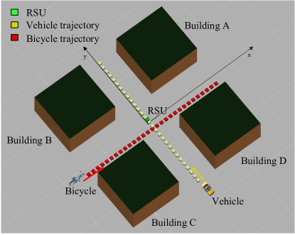
Figure 2: The ray-tracing simulation environment with a single RSU at the center of the intersection with location $[0\,\text{m},0\,\text{m},10\,\text{m}]^{\mathsf{T}}$, a vehicle moves from down to up (alongside the line $x=1.6\,\text{m}$), a bicycle moves from left to right (alongside the line $y=-7\,\text{m}$), and four buildings.

V-B Simulation Environment

Both scenarios are simulated using the REMCOM Wireless InSite®ray-tracer [32]. In Scenario 1, illustrated in Fig. 2, the RSU is located at the center of the intersection with location $[0\,\text{m},0\,\text{m},10\,\text{m}]^{\mathsf{T}}$. Two UEs are a vehicle and a bicycle. The vehicle moves alongside the vehicle lane (with its antenna at the height of $1.5\,\text{m}$), where the lane is from $[1.6\,\text{m},-70\,\text{m},0\,\text{m}]^{\mathsf{T}}$ to $[1.6\,\text{m},70\,\text{m},0\,\text{m}]^{\mathsf{T}}$. The bicycle moves alongside the bicycle lane (with its antenna at the height of $1\,\text{m}$), where the lane is from $[-70\,\text{m},-7\,\text{m},0\,\text{m}]^{\mathsf{T}}$ to $[70\,\text{m},-7\,\text{m},0\,\text{m}]^{\mathsf{T}}$. The four buildings are $50\,\text{m}$ long, $50\,\text{m}$ wide, and $30\,\text{m}$ high, with their centers located at $[\pm 45\,\text{m},\pm 45\,\text{m},15\,\text{m}]^{\mathsf{T}}$, respectively. All the RSU and the UEs are equipped with a single omnidirectional antenna. Every transmission interval, the RSU sends signals to the UEs via the propagation environment, but there is no communication between two UEs. In Scenario 2, there is no RSU, so that the vehicle sends signals to the bicycle every time step. The vehicle starts at $[1.6\,\text{m},-70\,\text{m},1.5\,\text{m}]^{\mathsf{T}}$, and moves to the end of the vehicle lane at $[1.6\,\text{m},70\,\text{m},1.5\,\text{m}]^{\mathsf{T}}$ with a speed of $14\,\text{m/s}$, and the bicycle starts at $[-16.4\,\text{m},-7\,\text{m},1\,\text{m}]^{\mathsf{T}}$ alongside the bicycle lane with a speed of $4.0\,\text{m/s}$. Then, the collision can occur after $4.5\,\text{s}$.

In terms of signal parameters, the carrier frequency is $5.9~{}\text{GHz}$. We consider the OFDM pilot signals with $12$ symbols with a constant amplitude, and $20~{}\text{MHz}$ total bandwidth with $167$ subcarriers and $120~{}\text{kHz}$ subcarrier spacing, corresponding to a pilot duration of $100.2~{}\text{us}$. The transmitted power is $10~{}\text{dBm}$, the noise spectral density is $-174~{}\text{dBm/Hz}$, and the receiver noise figure is $8~{}\text{dB}$. RTT measurements are generated every 100 ms.

For both scenarios, we evaluate the ranging performance by the root mean squared error (RMSE) over 100 Monte Carlo simulations, where each estimate can be acquired by firstly generating signals via (1) with Ray-tracing data, applying the ToA estimation in Section IV-A and converting the estimates into distances. We also compare the RMSEs with three range error bounds, obtained by taking the square root of the bound on the error variance of the ToA and multiplying with the speed of light. This leads to the LoS-only REB, the all-paths REB, and the proposed WAA REB. All codes were written in MATLAB R2018b, and simulations and experiments were run on a Lenovo ThinkPad T480s with a 1.8 GHz 4-Core Intel Core i7-8850U processor and 24 Gb memory.

Figure 3: Scenario 1 (vehicle): Comparison among the RMSE of estimated range between the vehicle and the RSU and three REBs.

Figure 4: Scenario 1 (bicycle): Comparison among the RMSE of the estimated range between the bicycle and the RSU and three REBs.

V-C Results and Discussion

Fig. 3 and Fig. 4 show the RMSE performance of the ranging to the vehicle and bicycle, respectively for Scenario 1. Fig. 5 shows the RMSE for Scenario 2 (without RSU). With respect to the positioning requirements, we note that for Scenario 1, within about 40 m from the RSU, the moderate accuracy (1–3 m) requirement can be exceeded. For Scenario 2, moderate accuracy is also attainable when vehicle and bicycle are sufficiently close to each-other.

Since the three figures exhibit a similar trend, we focus our discussion on Fig. 3. First of all, we note that the WAA REB is more reasonable than the LoS REB and the all-paths REB. This is because the LoS-only REB only considers the LoS path, which is overly optimistic, while the all-paths REB assumes all paths are resolvable, which leads to unreasonable results. The two bounds differ with 1–3 orders of magnitude, where the LoS-only REB promises sub-cm accuracy, while the all-paths REB varies from infinite error down to about 10 cm. On the other hand, the proposed WAA REBs takes the path non-resolvability into consideration and matches the estimator’s performance well. Secondly, we observe that the LoS and all-paths REBs decrease with the UE approaching the RSU, because the LoS path increases in power. In contrast, the algorithm and the WAA REB exhibit different behavior: around $y=-39.2\,\text{m}$ in Fig. 3, the WAA REBs rapidly drops when approaching the RSU. This effect is caused by the sudden disappearance of strong NLoS paths caused by the buildings, which in turn alleviates the inter-path interference. For example, the vehicle always has strong reflection paths from the buildings C and D at very beginning, but the buildings C and D cannot reflect any paths to vehicles anymore after $[1.6\,\text{m},-39.2\,\text{m},1.5\,\text{m}]^{\mathsf{T}}$, and the rest NLoS paths are relatively weak, thus the LoS becomes more dominate and the WAA REB drops accordingly. Later, when the vehicle starts to receive reflections from buildings A and B, the WAA REB will have a sudden increase. A second interesting effect appears when the the vehicle is in close proximity to the RSU (for $|y|<30\,\text{m}$). As the vehicle approaches the RSU, the WAA increases, in sharp contrast to the LoS-only and all-paths REBs. This effect is due to the ground reflection. Because of the limited bandwidth, the ground reflection always falls in the LoS resolution cell. Close to the RSU, the ground reflection is relatively strong with an amplitude of around 50% of the LoS path and an excess delay over $1~{}\text{m}$. Combined, this leads to a significant bias. This result shows that multiple antennas should be deployed to suppress ground reflections when bandwidth is limited.

Figure 5: Scenario 2: Comparison among the RMSE of the estimated range between the vehicle and the bicycle and three REBs.

VI Conclusions

In this paper, we focus on the analysis of sidelink V2X positioning towards 3GPP Release 18 in sub-6 GHz, where a novel methodology based on Fisher information analysis to predict positioning performance in a multipath propagation environment is provided, and the sidelink positioning and the method for positioning performance prediction are evaluated for two common urban scenarios occurring at an intersection using ray-tracing data. Our results indicate that the proposed WAA REB can predict the positioning performance better than the conventional bounds from the literature, since both multipath and the path non-resolvability are considered. The results indicate that biases due to multipath are the main cause of the error. Nevertheless, sub-meter accuracy was achievable, even in a complex urban scenario, when the transmitter and the receiver are sufficiently close. The impact of ground reflection was studied and found to be an important error source.

VII Acknowledgments

This work was partially supported by MSCA-IF grant 888913 (OTFS-RADCOM), and by the Wallenberg AI, Autonomous Systems and Software Program (WASP) funded by Knut and Alice Wallenberg Foundation. The authors wish to thank Remcom for providing Wireless InSite®ray-tracer.

References

- [1] T. Wild, V. Braun, and H. Viswanathan, “Joint design of communication and sensing for beyond 5G and 6G systems,” IEEE Access, vol. 9, pp. 30 845–30 857, 2021.
- [2] O. Kanhere and T. S. Rappaport, “Position location for futuristic cellular communications: 5G and beyond,” IEEE Communications Magazine, vol. 59, no. 1, pp. 70–75, 2021.
- [3] H. Wymeersch et al., “Localisation and sensing use cases and gap analysis,” Hexa-X project Deliverable D3.1, v1.4, 2022. [Online]. Available: https://hexa-x.eu/deliverables/
- [4] 3GPP, “Study on expanded and improved NR positioning,” TR 38.859, Technical Report 0.1.0, 2022.
- [5] 3GPP, “Study on scenarios and requirements of in-coverage, partial coverage, and out-of-coverage NR positioning use cases,” TR 38.845, Technical Report 17.0.0, 2021.
- [6] S.-W. Ko, H. Chae, K. Han, S. Lee, D.-W. Seo, and K. Huang, “V2X-based vehicular positioning: Opportunities, challenges, and future directions,” IEEE Wireless Communications, vol. 28, no. 2, pp. 144–151, 2021.
- [7] S. Bartoletti, H. Wymeersch, T. Mach, O. Brunnegrd, D. Giustiniano, P. Hammarberg, M. F. Keskin, J. O. Lacruz, S. M. Razavi, J. Rönnblom, et al., “Positioning and sensing for vehicular safety applications in 5G and beyond,” IEEE Communications Magazine, vol. 59, no. 11, pp. 15–21, 2021.
- [8] M. Säily, O. N. Yilmaz, D. S. Michalopoulos, E. Pérez, R. Keating, and J. Schaepperle, “Positioning technology trends and solutions toward 6G,” in IEEE International Symposium on Personal, Indoor and Mobile Radio Communications (PIMRC), 2021.
- [9] Y. Lu, M. Koivisto, J. Talvitie, E. Rastorgueva-Foi, T. Levanen, E. S. Lohan, and M. Valkama, “Joint positioning and tracking via NR sidelink in 5G-empowered industrial IoT: Releasing the potential of V2X technology,” arXiv preprint arXiv:2101.06003, 2021.
- [10] A. Bazzi, G. Cecchini, M. Menarini, B. M. Masini, and A. Zanella, “Survey and perspectives of vehicular Wi-Fi versus sidelink cellular-V2X in the 5G era,” Future Internet, vol. 11, no. 6, p. 122, 2019.
- [11] Q. Liu, P. Liang, J. Xia, T. Wang, M. Song, X. Xu, J. Zhang, Y. Fan, and L. Liu, “A highly accurate positioning solution for C-V2X systems,” Sensors, vol. 21, no. 4, p. 1175, 2021.
- [12] J. A. del Peral-Rosado, M. A. Barreto-Arboleda, F. Zanier, G. Seco-Granados, and J. A. López-Salcedo, “Performance limits of V2I ranging localization with LTE networks,” in IEEE Workshop on Positioning, Navigation and Communications (WPNC), 2017.
- [13] M. A. Hossain, I. Elshafiey, and A. Al-Sanie, “High accuracy GPS-free vehicular positioning based on V2V communications and RSU-assisted DOA estimation,” in IEEE-GCC Conference and Exhibition, 2017.
- [14] A. Kakkavas, M. H. C. Garcia, R. A. Stirling-Gallacher, and J. A. Nossek, “Multi-array 5G V2V relative positioning: Performance bounds,” in IEEE Global Communications Conference (GLOBECOM), 2018, pp. 206–212.
- [15] N. Decarli, S. Bartoletti, and B. M. Masini, “Joint communication and sensing in 5G-V2X vehicular networks,” in IEEE Mediterranean Electrotechnical Conference (MELECON), 2022, pp. 295–300.
- [16] S. Ma, F. Wen, X. Zhao, Z.-M. Wang, and D. Yang, “An efficient V2X based vehicle localization using single RSU and single receiver,” IEEE Access, vol. 7, pp. 46 114–46 121, 2019.
- [17] Q. Liu, R. Liu, Z. Wang, L. Han, and J. S. Thompson, “A V2X-integrated positioning methodology in ultradense networks,” IEEE Internet of Things Journal, vol. 8, no. 23, pp. 17 014–17 028, 2021.
- [18] A. Fouda, R. Keating, and A. Ghosh, “Dynamic selective positioning for high-precision accuracy in 5G NR V2X networks,” in IEEE Vehicular Technology Conference (VTC2021-Spring), 2021.
- [19] “System architecture and solution development; high-accuracy positioning for C-V2X,” 5GAA Automotive Association Technical Report, 2021. [Online]. Available: http://www.5gaa.org
- [20] 3GPP, “Technical specification group radio access network; study on evaluation methodology of new vehicle-to-everything (V2X) use cases for LTE and NR,” TR 37.885, Technical Report 15.3.0, 2019.
- [21] C. R. Berger, B. Demissie, J. Heckenbach, P. Willett, and S. Zhou, “Signal processing for passive radar using OFDM waveforms,” IEEE Journal of Selected Topics in Signal Processing, vol. 4, no. 1, pp. 226–238, 2010.
- [22] A. Behravan, V. Yajnanarayana, M. F. Keskin, H. Chen, T. E. A. Deep Shrestha, T. Svensson, K. Schindhelm, A. Wolfgang, S. Lindberg, and H. Wymeersch, “Positioning and sensing in 6G: Gaps, challenges, and opportunities,” IEEE Vehicular Technology Magazine (under review), 2022.
- [23] H. L. V. Trees, Detection, Estimation, and Modulation Theory. John Wiley & Sons, New York, 2004.
- [24] Y. Shen and M. Z. Win, “Fundamental limits of wideband localization— part I: A general framework,” IEEE Transactions on Information Theory, vol. 56, no. 10, pp. 4956–4980, 2010.
- [25] S. Mercier, S. Bidon, D. Roque, and C. Enderli, “Comparison of correlation-based OFDM radar receivers,” IEEE Transactions on Aerospace and Electronic Systems, vol. 56, no. 6, pp. 4796–4813, 2020.
- [26] C. Sturm and W. Wiesbeck, “Waveform design and signal processing aspects for fusion of wireless communications and radar sensing,” Proceedings of the IEEE, vol. 99, no. 7, pp. 1236–1259, July 2011.
- [27] M. Braun, “OFDM radar algorithms in mobile communication networks,” Karlsruher Institutes für Technologie, 2014.
- [28] Y. Qi, H. Kobayashi, and H. Suda, “On time-of-arrival positioning in a multipath environment,” IEEE Transactions on Vehicular Technology, vol. 55, no. 5, pp. 1516–1526, 2006.
- [29] S. Parkvall, Y. Blankenship, R. Blasco, E. Dahlman, G. Fodor, S. Grant, E. Stare, and M. Stattin, “5G NR release 16: Start of the 5G evolution,” IEEE Communications Standards Magazine, vol. 4, no. 4, pp. 56–63, 2020.
- [30] H. Bagheri, M. Noor-A-Rahim, Z. Liu, H. Lee, D. Pesch, K. Moessner, and P. Xiao, “5G NR-V2X: Toward connected and cooperative autonomous driving,” IEEE Communications Standards Magazine, vol. 5, no. 1, pp. 48–54, 2021.
- [31] S. Zhu and Z. Ding, “A simple approach of range-based positioning with low computational complexity,” IEEE Transactions on Wireless Communications, vol. 8, no. 12, pp. 5832–5836, 2009.
- [32] Remcom. Wireless InSite - 3D Wireless Prediction Software. Accessed: Oct 9, 2022). [Online]. Available: https://www.remcom.com/wireless-insite-em-propagation-software