Cumulants from short-range correlations and baryon number conservation - next-to-leading order

Abstract

We calculate the baryon number cumulants within acceptance with short-range correlations and global baryon number conservation in terms of cumulants in the whole system without baryon conservation. We extract leading and next-to-leading order terms of the large baryon number limit approximation. Our results extend the findings of Refs. Vovchenko et al. (2020a); Barej and Bzdak (2022). These approximations are checked to be very close to the exact results.

I Introduction

The phase diagram of the strongly interacting matter is not yet well explored. Especially, the search for the first-order phase transition between the hadronic matter and quark-gluon plasma, and the corresponding critical endpoint, which are predicted by the effective models, remains a big challenge in high-energy physics Stephanov (2004); Braun-Munzinger and Wambach (2009); Braun-Munzinger et al. (2016); Bzdak et al. (2020). It is known that the fluctuations of conserved charges, e.g., baryon number, electric charge, or strangeness are sensitive to the relevant critical phenomena. Therefore, many theoretical projects, as well as experiments in relativistic heavy-ion collisions, have been established to study them Jeon and Koch (2000); Asakawa et al. (2000); Gazdzicki et al. (2004); Gorenstein et al. (2004); Stephanov (2004); Koch et al. (2005); Stephanov (2009); Cheng et al. (2009); Fu et al. (2010); Skokov et al. (2011); Stephanov (2011); Karsch and Redlich (2011); Schaefer and Wagner (2012); Chen et al. (2011); Luo et al. (2012); Zhou et al. (2012); Wang and Yang (2012); Herold et al. (2016); Luo and Xu (2017); Szymański et al. (2020); Ratti (2019).

Cumulants are commonly used to quantify these fluctuations because they naturally appear in statistical mechanics Stephanov (2009); Behera (2019); Acharya et al. (2020); Skokov et al. (2012); Braun-Munzinger et al. (2012); Bzdak and Koch (2012); Braun-Munzinger et al. (2017); Adamczyk et al. (2018); Adare et al. (2016). On the other hand, the factorial cumulants might be easier to interpret since they represent integrated multiparticle correlation functions Botet and Ploszajczak (2002); Ling and Stephanov (2016); Bzdak et al. (2017a, 2020); Adamczyk et al. (2014); Bzdak et al. (2017a, 2018); Bzdak and Koch (2019); Adamczewski-Musch et al. (2020a); Abdallah et al. (2021); Vovchenko et al. (2022). However, both the cumulants and factorial cumulants are affected also by fluctuations unrelated to the phase transition, for instance, the impact parameter fluctuations and the conservation laws, e.g., the baryon number conservation Skokov et al. (2013); Braun-Munzinger et al. (2017); Bzdak et al. (2017b); Adamczewski-Musch et al. (2020b); Kitazawa and Asakawa (2012); Bzdak et al. (2013); Braun-Munzinger et al. (2017); Rogly et al. (2019); Braun-Munzinger et al. (2019); Acharya et al. (2020); Savchuk et al. (2020); Braun-Munzinger et al. (2021); Vovchenko et al. (2022).

In our previous paper Barej and Bzdak (2022), we derived analytically the baryon number factorial cumulant generating function in a finite acceptance, assuming short-range correlations and global baryon number conservation. Among other results, we calculated the factorial cumulants and cumulants within the limit of small short-range correlation strengths, $\alpha_{k}$, and large baryon number, $B$. We also reproduced the relations between cumulants in a subsystem with all correlations and cumulants in the whole system without baryon conservation, initially obtained in Ref. Vovchenko et al. (2020a).

In this paper, we extend this study and present a method of obtaining the first correction to the cumulants in the large baryon number limit. We also note that the short-range correlations strengths cannot assume arbitrary values. Finally, we compare our approximate analytic results with the brute-force computations.

In the next Section, we show our method of extracting the baryon number cumulants assuming short-range correlations and global baryon number conservation. Then, we present the leading-order and next-to-leading order terms of cumulants in the subsystem with all correlations expanded in the large $B$ limit with respect to cumulants in the whole system without baryon conservation. This is our main result. In the fourth section, we show how our approximate analytic formulas work by comparison with the exact results. The alternative approach and the discussion on the limitations of $\alpha_{k}$’s originating from the probability theory can be found in the Appendixes.

II Method

II.1 Previous study

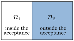
In our previous paper Barej and Bzdak (2022), we considered a system of fixed volume and some number of particles of one kind, say baryons. We divided it into two subsystems (inside and outside the acceptance, see Fig. 1) which can exchange particles. Let $P_{1}(n_{1})$ and $P_{2}(n_{2})$ be the probabilities that there are $n_{1}$ particles in the first subsystem and $n_{2}$ particles in the second one, respectively. The probability that there are $n_{1}$ particles in the first subsystem and $n_{2}$ particles in the second one is $P(n_{1},n_{2})=P_{1}(n_{1})P_{2}(n_{2})$ if there are no correlations between the two subsystems or (approximately) if there are only short-range correlations. Assuming the global baryon number conservation, this probability becomes

$$P_{B}(n_{1},n_{2})=A\;P_{1}(n_{1})P_{2}(n_{2})\delta_{n_{1}+n_{2},B}\,,$$ (1)

where $A$ is the normalization constant and $B$ is the total baryon number. In this case, the probability that there are $n_{1}$ particles in the first subsystem (within acceptance) reads

$$P_{B}(n_{1})=\sum_{n_{2}=0}^{\infty}P_{B}(n_{1},n_{2})\,.$$ (2)

Figure 1: The system is divided into two subsystems with $n_{1}$ particles in the first subsystem (inside the acceptance) and $n_{2}$ particles in the second one (outside the acceptance).

Then, we calculated the factorial cumulant generating function for the first subsystem with baryon number conservation:

$$G_{(1,B)}(z)=\ln\left[\frac{A}{B!}\left.\frac{d^{B}}{dx^{B}}\exp\left(\sum_{k=1}^{\infty}\frac{(xz-1)^{k}\hat{C}_{k}^{(1)}+(x-1)^{k}\hat{C}_{k}^{(2)}}{k!}\right)\right|_{x=0}\right]\,,$$ (3)

where

$$\begin{split}\hat{C}_{k}^{(1)}&=\langle n_{1}\rangle\alpha_{k}=f\langle N\rangle\alpha_{k}\,,\\ \hat{C}_{k}^{(2)}&=\langle n_{2}\rangle\alpha_{k}=(1-f)\langle N\rangle\alpha_{k}\end{split}$$ (4)

are the short-range factorial cumulants in the first and the second subsystem, respectively (see Barej and Bzdak (2022); Bzdak et al. (2020)), for the multiplicity distribution without global baryon conservation. Here $\langle N\rangle=\langle n_{1}\rangle+\langle n_{2}\rangle$ is the mean total number of particles in the system, $f=\langle n_{1}\rangle/\langle N\rangle$ is a fraction of particles in the first subsystem, and $\alpha_{k}$ describes the strength of $k$-particle short-range correlations ($\alpha_{1}=1$). We assumed that the total average number of particles $\langle N\rangle=\langle n_{1}\rangle+\langle n_{2}\rangle=B$. Introducing the global baryon number conservation further requires that the total number of particles $N=n_{1}+n_{2}$ equals $B$ in every event.

Using the factorial cumulant generating function (3), one can obtain the factorial cumulants in the first subsystem (within acceptance) with baryon number conservation:

$$\hat{C}_{k}^{(1,B)}=\left.\frac{d^{k}}{dz^{k}}G_{(1,B)}(z)\right|_{z=1}\,.$$ (5)

We obtained Barej and Bzdak (2022) the analytic as well as approximate formulas for the factorial cumulants in the simple case of only two-particle short-range correlations. Then, we also derived the approximate factorial cumulants and cumulants in the limit of $B\to\infty$ assuming multiparticle short-range correlations. These results reproduced the findings of Ref. Vovchenko et al. (2020a) obtained originally using a different approach.

II.2 Next-to-leading order correction

We extend the previous study and obtain the next-to-leading order terms of the expansion of the cumulants in the limit of $B\to\infty$. We derive the relevant expressions in two different ways. One method, presented in Appendix A, is based on analyzing the first few terms of the expansions, deducing the following terms, and then summing the infinite series. Here we present another method that is simpler.

In order to make the computations, we approximate Eq. (3) with Eq. (4) by

$$G_{(1,B)}(z)\approx\ln\left[\frac{A}{B!}\left.\frac{d^{B}}{dx^{B}}\left[\exp\left((xz-1)fB+(x-1)\bar{f}B\right)\sum_{m=0}^{M}\frac{V^{m}}{m!}\right]\right|_{x=0}\right]\,,$$ (6)

where $\bar{f}=1-f$ and

$$V=\sum_{k=2}^{K}\left(\frac{(xz-1)^{k}}{k!}fB\alpha_{k}+\frac{(x-1)^{k}}{k!}\bar{f}B\alpha_{k}\right)\,,$$ (7)

with $M$ and $K$ being the upper limits. Note that in Eq. (7) we allow for up to $K$-particle short-range correlations.

To calculate the $B$th derivative with respect to $x$ in Eq. (6), we use the general Leibnitz formula as described in Ref. Barej and Bzdak (2022). In this way we evaluate the factorial cumulant generating function (6) and then the factorial cumulants (5). Having the factorial cumulants, we calculate the cumulants according to

$$\kappa_{n}=\sum_{k=1}^{n}S(n,k)\hat{C}_{k}\,,$$ (8)

where $S(n,k)$ is the Stirling number of the second kind Friman and Redlich (2022). For instance, the second cumulant reads

$$\kappa_{2}^{(1,B)}=\langle n_{1}\rangle+\hat{C}_{2}^{(1,B)}\,,$$ (9)

where $\hat{C}_{1}^{(1,B)}=\kappa_{1}^{(1,B)}=\langle n_{1}\rangle=fB$.

The global (both subsystems combined) short-range factorial cumulants, without the baryon number conservation, are defined as (compare with Eqs. (4)):

$$\hat{C}_{n}^{(G)}=B\alpha_{n}\,.$$ (10)

The global cumulants without the baryon number conservation, $\kappa_{n}^{(G)}$, are obtained by Eq. (8).

As shown in Ref. Barej and Bzdak (2022), the cumulants, $\kappa_{n}^{(1,B)}$, can be expressed as a power series in terms of $B$ where the highest-order term is linear in $B$. Namely,

$$\kappa_{n}^{(1,B)}\approx\underbrace{\kappa_{n}^{(1,B,\text{LO})}}_{u_{n,1}B^{1}}+\underbrace{\kappa_{n}^{(1,B,\text{NLO})}}_{u_{n,0}B^{0}}+\underbrace{\kappa_{n}^{(1,B,\text{NNLO})}}_{u_{n,-1}B^{-1}}+\underbrace{\ldots}_{O(B^{-2})}\,,$$ (11)

where $\kappa_{n}^{(1,B,\text{LO})}$, $\kappa_{n}^{(1,B,\text{NLO})}$, and $\kappa_{n}^{(1,B,\text{NNLO})}$ denote the leading-order, next-to-leading-order, and next-to-next-to-leading-order terms of the power series in $B$, respectively.

Let us focus on the second cumulant. Using the method presented in Appendix A, we deduced that in order to extract LO and NLO terms, it is convenient to multiply $\kappa_{2}^{(1,B)}$ by $(\kappa_{2}^{(G)})^{2}=[B(1+\alpha_{2})]^{2}$. We define

$$\widetilde{\kappa}_{2}^{(1,B)}=\kappa_{2}^{(1,B)}(\kappa_{2}^{(G)})^{2}=\kappa_{2}^{(1,B)}[B(1+\alpha_{2})]^{2}\,.$$ (12)

Then, we expand $\widetilde{\kappa}_{2}^{(1,B)}$ into the power series in $\alpha_{k}$ up to the order of $M$, obtaining $\widetilde{\kappa}_{2}^{(1,B,\text{ser})}$:

$$\widetilde{\kappa}_{2}^{(1,B)}\approx\widetilde{\kappa}_{2}^{(1,B,\text{ser})}=u_{2,1}(1+\alpha_{2})^{2}B^{3}+u_{2,0}(1+\alpha_{2})^{2}B^{2}+\underbrace{\ldots}_{O(B)}\,.$$ (13)

The coefficients of the expansion are calculated as follows,

$$\begin{split}{u}_{2,1}&=\frac{1}{(1+\alpha_{2})^{2}}\lim_{B\to\infty}\frac{\widetilde{\kappa}_{2}^{(1,B,\text{ser})}}{B^{3}}\,,\\ {u}_{2,0}&=\frac{1}{(1+\alpha_{2})^{2}}\lim_{B\to\infty}\frac{\widetilde{\kappa}_{2}^{(1,B,\text{ser})}-{u}_{2,1}(1+\alpha_{2})^{2}B^{3}}{B^{2}}\,.\end{split}$$ (14)

Clearly, it is possible to extract even higher terms in an analogous way. Using Eqs. (8) and (10), we express these coefficients in terms of the global short-range cumulants (without the baryon conservation), $\kappa_{n}^{(G)}$.

The same technique is applied to obtain the leading and next-to-leading order terms of $\kappa_{3}^{(1,B)}$. Namely, we multiply $\kappa_{3}^{(1,B)}$ by $(\kappa_{2}^{(G)})^{2}$.

It turns out that $\kappa_{4}^{(1,B)}$ needs to be multiplied by $(\kappa_{2}^{(G)})^{4}$. Namely,

$$\widetilde{\kappa}_{4}^{(1,B)}=\kappa_{4}^{(1,B)}(\kappa_{2}^{(G)})^{4}=\kappa_{4}^{(1,B)}[B(1+\alpha_{2})]^{4}\,.$$ (15)

In this case, equations corresponding to Eqs. (13) and (14) read:

$$\widetilde{\kappa}_{4}^{(1,B)}\approx\widetilde{\kappa}_{4}^{(1,B,\text{ser})}=u_{4,1}(1+\alpha_{2})^{4}B^{5}+u_{4,0}(1+\alpha_{2})^{4}B^{4}+\underbrace{\ldots}_{O(B^{3})}\,,$$ (16)

and

$$\begin{split}{u}_{4,1}&=\frac{1}{(1+\alpha_{2})^{4}}\lim_{B\to\infty}\frac{\widetilde{\kappa}_{4}^{(1,B,\text{ser})}}{B^{5}}\,,\\ {u}_{4,0}&=\frac{1}{(1+\alpha_{2})^{4}}\lim_{B\to\infty}\frac{\widetilde{\kappa}_{4}^{(1,B,\text{ser})}-{u}_{4,1}(1+\alpha_{2})^{4}B^{5}}{B^{4}}\,.\end{split}$$ (17)

The results are computed using Mathematica software Wolfram Research Inc. .

III Results

The relations between cumulants in the first subsystem with all correlations, $\kappa_{n}^{(1,B)}$, vs. cumulants in the whole system without baryon conservation, $\kappa^{(G)}_{m}$, are given by:

$$\kappa_{1}^{(1,B)} =fB=f\kappa_{1}^{(G)}\,,$$ (18)

$$\kappa_{2}^{(1,B,\text{LO})} =\bar{f}f\kappa_{2}^{(G)}\,,$$ (19)

$$\kappa_{2}^{(1,B,\text{NLO})} =\frac{1}{2}\bar{f}f\frac{(\kappa^{(G)}_{3})^{2}-\kappa^{(G)}_{2}\kappa^{(G)}_{4}}{(\kappa^{(G)}_{2})^{2}}\,,$$ (20)

$$\kappa_{3}^{(1,B,\text{LO})} =\bar{f}f(1-2f)\kappa_{3}^{(G)}\,,$$ (21)

$$\kappa_{3}^{(1,B,\text{NLO})} =\frac{1}{2}f\bar{f}(1-2f)\frac{\kappa^{(G)}_{3}\kappa^{(G)}_{4}-\kappa^{(G)}_{2}\kappa^{(G)}_{5}}{(\kappa^{(G)}_{2})^{2}}\,, \,.$$ (22)

$$\kappa_{4}^{(1,B,\text{LO})} =f\bar{f}\left[\kappa^{(G)}_{4}-3f\bar{f}\left(\kappa^{(G)}_{4}+\frac{(\kappa^{(G)}_{3})^{2}}{\kappa^{(G)}_{2}}\right)\right]\,,$$ (23)

$$\kappa_{4}^{(1,B,\text{NLO})} =\frac{1}{2}f\bar{f}\left\{\frac{\kappa^{(G)}_{3}\kappa^{(G)}_{5}-\kappa^{(G)}_{2}\kappa^{(G)}_{6}}{(\kappa^{(G)}_{2})^{2}}\right.$$ (24)

$$+3f\bar{f}\left[\frac{2(\kappa^{(G)}_{3})^{4}-5\kappa^{(G)}_{2}(\kappa^{(G)}_{3})^{2}\kappa^{(G)}_{4}+(\kappa^{(G)}_{2})^{2}\kappa^{(G)}_{3}\kappa^{(G)}_{5}}{(\kappa^{(G)}_{2})^{4}}\left.+\frac{(\kappa^{(G)}_{4})^{2}+\kappa^{(G)}_{2}\kappa^{(G)}_{6}}{(\kappa^{(G)}_{2})^{2}}\right]\right\}\,.$$

The leading-order terms, $\kappa_{n}^{(1,B,\text{LO})}$, were already obtained in Barej and Bzdak (2022) and originally in Vovchenko et al. (2020a). The final results for $\kappa_{2}^{(1,B,NLO)}$ and $\kappa_{3}^{(1,B,NLO)}$ are obtained already for $M=3$ and $K=5$ (see Eqs. (6) and (7)). We have checked (up to $M=7$ and $K=7$) that when increasing $M$ or $K$ the results remain unchanged. The final results for $\kappa_{4}^{(1,B,NLO)}$ are obtained for $M=5$ and $K=6$. We have verified them up to $M=6$ and $K=7$ as well as up to $M=7$ and $K=6$. When further increasing $M$ or $K$ the computations become challenging.

IV Examples

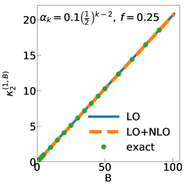
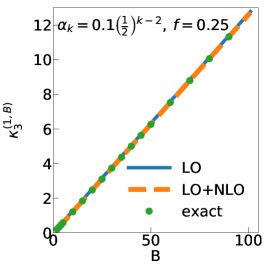
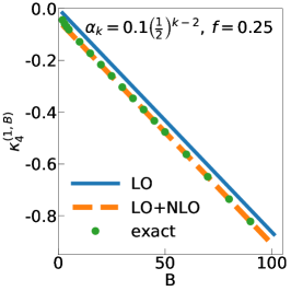
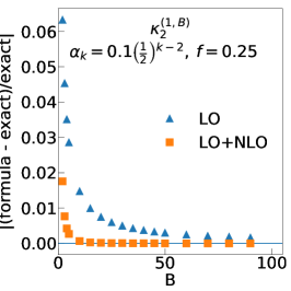
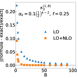
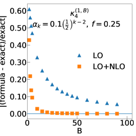
We calculate the cumulants for the selected values of the $k$-particle short-range correlation strengths, $\alpha_{k}$’s, the fraction of particle number in the first subsystem, $f$, and the baryon number, $B$. We do this in three different ways. Firstly, we calculate the cumulants by a straightforward differentiation using Equations 3–5 (exact results). Secondly, we calculate them using only the leading-order terms (Eqs. (19), (21), and (23)). Finally, we calculate them by applying both the leading- and next-to-leading order terms.

The $k$-particle short-range correlations are typically small and the higher-order ones are expected to be smaller than the lower-order ones. Thus, as an example, we study the case of $\alpha_{k}=0.1\left(\frac{1}{2}\right)^{k-2}$, $k=2,3,...,6$, $\alpha_{1}=1$, $f=0.25$. In Fig. 2, we show the cumulants as a function of the baryon number, $B$, calculated in three ways and we also present the relative errors with respect to the exact ones. We see that including the NLO term gives a significantly better approximation of the exact results. We have also studied other values of parameters and the observations are consistent. We note that for $f=0.5$, $\kappa^{(1,B)}_{3}$ vanishes for all values of $B$ Bzdak and Koch (2017); Vovchenko et al. (2020b).

It is worth mentioning that $\alpha_{k}$ cannot be arbitrary. We discuss this issue in Appendix B.

Figure 2: Upper plots: The second (left), third (middle), and fourth (right) cumulant in the first subsystem (within acceptance) with the short-range correlations and baryon number conservation as a function of $B$. $\alpha_{k}=0.1\left(\frac{1}{2}\right)^{k-2}$, $k=2,3,...,6$, $\alpha_{1}=1$, $f=0.25$. “LO” denotes the results obtained from the leading-order terms (Eqs. (19), (21), and (23)). “LO+NLO” denotes the results obtained using the leading-order and next-to-leading-order terms (Eqs. (19), (21), (23) plus Eqs. (20), (22), and (24)). The “exact” points denote the direct calculation from Equations 3–5. The exact results are presented for $B=2,3,4,5,10,15,20,25,30,35,40,45,50,60,70,80,90$. Lower plots: The relative error for each $B$. “formula” can be a result of LO or LO+NLO. As seen, the use of the next-to-leading order term improves the results significantly.

V Comments and summary

In this paper, we have extended the results of Ref. Barej and Bzdak (2022). We have presented the method of obtaining successive terms of the large $B$ limit expansion of the baryon number cumulants in the subsystem with the short-range correlations and global baryon number conservation. We have expressed them by the cumulants in the whole system without baryon number conservation. The newly obtained next-to-leading order terms have improved the approximation as seen in Section IV.

In this calculation, we have neglected antibaryons, which makes our results applicable to lower collision energies. We have presented baryon number cumulants, whereas typically in the experiments the proton (net-proton) number cumulants are measured because it is more challenging to detect neutrons.

An interesting but rather challenging extension of this method would be to take into account also antibaryons, as well as other long-range correlations.

Appendix A The series expansion approach

Here we present another way of obtaining the leading and next-to-leading order terms of the $B$ power series expansion of the cumulants.

We obtain the factorial cumulants, $\hat{C}_{n}^{(1,B)}$, in the same way as in Sec. II.2. Then, we expand them into the $\alpha_{k}$ power series up to the order of $M$. As shown in Barej and Bzdak (2022), $\hat{C}_{n}^{(1,B)}$ can be written as a power series in terms of $B$,

$$\hat{C}_{n}^{(1,B)}\approx\hat{C}_{n}^{(1,B,\text{ser})}=\underbrace{\hat{C}_{n}^{(1,B,\text{LO})}}_{v_{n,1}B^{1}}+\underbrace{\hat{C}_{n}^{(1,B,\text{NLO})}}_{v_{n,0}B^{0}}+\underbrace{\hat{C}_{n}^{(1,B,\text{NNLO})}}_{v_{n,-1}B^{-1}}+\underbrace{\ldots}_{O(B^{-2})}\,,$$ (25)

where $\hat{C}_{n}^{(1,B,\text{LO})}$, $\hat{C}_{n}^{(1,B,\text{NLO})}$, and $\hat{C}_{n}^{(1,B,\text{NNLO})}$ denote the leading, next-to-leading, and next-to-next-to-leading order terms. The coefficients, $v_{n,1}$ and $v_{n,0}$, are calculated as follows:

$$\begin{split}v_{n,1}&=\lim_{B\to\infty}\frac{\hat{C}_{n}^{(1,B,\text{ser})}}{B}\,,\\ v_{n,0}&=\lim_{B\to\infty}\left(\hat{C}_{n}^{(1,B,\text{ser})}-v_{n,1}B\right)\,.\end{split}$$ (26)

The subsequent coefficients can be obtained in a similar way. Note that the leading-order terms, $\hat{C}_{n}^{(1,B,\text{LO})}$, were presented in Ref. Barej and Bzdak (2022).

We calculate the LO and NLO terms of cumulants from factorial cumulants using Eq. (8). For instance,

$$\begin{split}\kappa_{3}^{(1,B)}&=\langle n_{1}\rangle+3\hat{C}_{2}^{(1,B)}+\hat{C}_{3}^{(1,B)}\\ &\approx fB+3\left(\hat{C}_{2}^{(1,B,\text{LO})}+\hat{C}_{2}^{(1,B,\text{NLO})}\right)+\left(\hat{C}_{3}^{(1,B,\text{LO})}+\hat{C}_{3}^{(1,B,\text{NLO})}\right)\\ &=\underbrace{\left(fB+3\hat{C}_{2}^{(1,B,\text{LO})}+\hat{C}_{3}^{(1,B,\text{LO})}\right)}_{\kappa_{3}^{(1,B,\text{LO})}}+\underbrace{\left(3\hat{C}_{2}^{(1,B,\text{NLO})}+\hat{C}_{3}^{(1,B,\text{NLO})}\right)}_{\kappa_{3}^{(1,B,\text{NLO})}}\,,\end{split}$$ (27)

where $\hat{C}_{1}^{(1,B)}=\kappa_{1}^{(1,B)}=\langle n_{1}\rangle=fB$.

Next, we express $\kappa_{n}^{(1,B,\text{LO})}$ and $\kappa_{n}^{(1,B,\text{NLO})}$ by the global (in the whole system) factorial cumulants, $\hat{C}_{n}^{(G)}$, with short-range correlations but without baryon number conservation, defined in Eq. (10), and then, by the global cumulants without the baryon number conservation, $\kappa_{n}^{(G)}$.

For the Poisson distribution, all the cumulants $\kappa_{n}^{(G)}=\langle N\rangle=B$. Therefore,

$$\bar{\kappa}_{n}^{(G)}=\frac{\kappa_{n}^{(G)}}{B}-1$$ (28)

describes the deviation from the Poisson distribution. We expect it to be small (for example, $\bar{\kappa}_{2}^{(G)}=\alpha_{2}$) and thus we express $\kappa_{n}^{(1,B,\text{LO})}$ and $\kappa_{n}^{(1,B,\text{NLO})}$ in terms of $\bar{\kappa}_{m}^{(G)}$.

We note that when using Eqs. (6) and (7), the final results for $\kappa_{1}^{(1,B)}$, $\kappa_{2}^{(1,B,\text{LO})}$, and $\kappa_{3}^{(1,B,\text{LO})}$ are obtained already for $M=1$ and $K=3$, and an increase of $M$ and $K$ does not modify the results. In other cases, we obtain more and more terms when increasing $M$. However, we can deduce empirically the series in $\bar{\kappa}^{(G)}_{2}$ using the first few terms and confirm them by increasing $M$ and $K$ in Eqs. (6) and (7). We have performed the computations up to $M=8$, $K=6$, and also up to $M=4$, $K=8$. By summing the series up to infinity, we derive the finite analytic formulas for LO and NLO terms of the cumulants, and we obtain the same results as given by Equations 18–24.

A.1 $\kappa_{2}^{(1,B)}$ and $\kappa_{3}^{(1,B)}$

The leading-order terms of $\kappa_{2}^{(1,B)}$ and $\kappa_{3}^{(1,B)}$ read Barej and Bzdak (2022); Vovchenko et al. (2020a):

$$\begin{split}\kappa_{2}^{(1,B,\text{LO})}&=\bar{f}f\kappa_{2}^{(G)}\,,\\ \kappa_{3}^{(1,B,\text{LO})}&=\bar{f}f(1-2f)\kappa_{3}^{(G)}\,.\end{split}$$ (29)

The NLO term of $\kappa_{2}^{(1,B)}$ is given by the power series in $\bar{\kappa}^{(G)}_{2}$. This is understandable since in the process of computation we expand the factorial cumulants into power series about $\alpha_{k}=0$ up to order $M$ (see Sec. II.2). The NLO term of the second cumulant with $M=8$ is given by

$$\begin{split}\kappa_{2}^{(1,B,\text{NLO})}&\approx\frac{1}{2}f\bar{f}\biggl{[}-\bar{\kappa}^{(G)}_{2}+2(\bar{\kappa}^{(G)}_{2})^{2}-3(\bar{\kappa}^{(G)}_{2})^{3}+4(\bar{\kappa}^{(G)}_{2})^{4}-5(\bar{\kappa}^{(G)}_{2})^{5}+6(\bar{\kappa}^{(G)}_{2})^{6}-7(\bar{\kappa}^{(G)}_{2})^{7}+8(\bar{\kappa}^{(G)}_{2})^{8}\\ &\phantom{=\frac{1}{2}f}+2\bar{\kappa}^{(G)}_{3}\left(1-2\bar{\kappa}^{(G)}_{2}+3(\bar{\kappa}^{(G)}_{2})^{2}-4(\bar{\kappa}^{(G)}_{2})^{3}+5(\bar{\kappa}^{(G)}_{2})^{4}-6(\bar{\kappa}^{(G)}_{2})^{5}+7(\bar{\kappa}^{(G)}_{2})^{6}-8(\bar{\kappa}^{(G)}_{2})^{7}\right)\\ &\phantom{=\frac{1}{2}f}+(\bar{\kappa}^{(G)}_{3})^{2}\left(1-2\bar{\kappa}^{(G)}_{2}+3(\bar{\kappa}^{(G)}_{2})^{2}-4(\bar{\kappa}^{(G)}_{2})^{3}+5(\bar{\kappa}^{(G)}_{2})^{4}-6(\bar{\kappa}^{(G)}_{2})^{5}+7(\bar{\kappa}^{(G)}_{2})^{6}\right)\\ &\phantom{=\frac{1}{2}f}+\bar{\kappa}^{(G)}_{4}\left(-1+\bar{\kappa}^{(G)}_{2}-(\bar{\kappa}^{(G)}_{2})^{2}+(\bar{\kappa}^{(G)}_{2})^{3}-(\bar{\kappa}^{(G)}_{2})^{4}+(\bar{\kappa}^{(G)}_{2})^{5}-(\bar{\kappa}^{(G)}_{2})^{6}+(\bar{\kappa}^{(G)}_{2})^{7}\right)\biggr{]}\,.\end{split}$$ (30)

Here we recognize the series:

$$\begin{split}\kappa_{2}^{(1,B,\text{NLO})}&\approx\frac{1}{2}f\bar{f}\biggl{[}\sum_{n=1}^{N=8}n\left(-\bar{\kappa}^{(G)}_{2}\right)^{n}+2\bar{\kappa}^{(G)}_{3}\sum_{n=1}^{N=8}n\left(-\bar{\kappa}^{(G)}_{2}\right)^{n-1}+(\bar{\kappa}^{(G)}_{3})^{2}\sum_{n=1}^{N=7}n\left(-\bar{\kappa}^{(G)}_{2}\right)^{n-1}\\ &\phantom{=\frac{1}{2}f\bar{f}}-\bar{\kappa}^{(G)}_{4}\sum_{n=1}^{N=8}\left(-\bar{\kappa}^{(G)}_{2}\right)^{n-1}\biggr{]}\,.\end{split}$$ (31)

Then, we assume that the next terms follow this pattern and we sum up with $N\to\infty$. We obtain

$$\begin{split}\kappa_{2}^{(1,B,\text{NLO})}&=\frac{1}{2}\bar{f}f\biggl{[}-\frac{\bar{\kappa}^{(G)}_{2}}{(1+\bar{\kappa}^{(G)}_{2})^{2}}+\frac{2\bar{\kappa}^{(G)}_{3}}{(1+\bar{\kappa}^{(G)}_{2})^{2}}+\frac{(\bar{\kappa}^{(G)}_{3})^{2}}{(1+\bar{\kappa}^{(G)}_{2})^{2}}-\frac{\bar{\kappa}^{(G)}_{4}}{1+\bar{\kappa}^{(G)}_{2}}\biggr{]}\\ &=-\frac{1}{2}\bar{f}f\frac{\bar{\kappa}^{(G)}_{2}-2\bar{\kappa}^{(G)}_{3}+\bar{\kappa}^{(G)}_{4}(1+\bar{\kappa}^{(G)}_{2})-(\bar{\kappa}^{(G)}_{3})^{2}}{(1+\bar{\kappa}^{(G)}_{2})^{2}}\,.\end{split}$$ (32)

We substitute back Eq. (28) and we obtain Eq. (20).

The case of the NLO term of $\kappa_{3}^{(1,B)}$ is similar. The result reads:

$$\begin{split}\kappa_{3}^{(1,B,\text{NLO})}&=\frac{1}{2}f\bar{f}(1-2f)\biggl{[}\sum_{n=1}^{N=8}n\left(-\bar{\kappa}^{(G)}_{2}\right)^{n}+\bar{\kappa}^{(G)}_{3}\sum_{n=1}^{N=8}n\left(-\bar{\kappa}^{(G)}_{2}\right)^{n-1}+\bar{\kappa}^{(G)}_{4}\sum_{n=1}^{N=8}n\left(-\bar{\kappa}^{(G)}_{2}\right)^{n-1}\\ &\phantom{=\frac{1}{2}f\bar{f}(1-2f)}+\bar{\kappa}^{(G)}_{3}\bar{\kappa}^{(G)}_{4}\sum_{n=1}^{N=7}n\left(-\bar{\kappa}^{(G)}_{2}\right)^{n-1}-\bar{\kappa}^{(G)}_{5}\sum_{n=1}^{N=8}\left(-\bar{\kappa}^{(G)}_{2}\right)^{n-1}\biggr{]}\,.\end{split}$$ (33)

By letting $N\to\infty$, we have

$$\begin{split}\kappa_{3}^{(1,B,\text{NLO})}&=\frac{1}{2}f\bar{f}(1-2f)\biggl{[}-\frac{\bar{\kappa}^{(G)}_{2}}{(1+\bar{\kappa}^{(G)}_{2})^{2}}+\frac{\bar{\kappa}^{(G)}_{3}}{(1+\bar{\kappa}^{(G)}_{2})^{2}}+\frac{\bar{\kappa}^{(G)}_{4}}{(1+\bar{\kappa}^{(G)}_{2})^{2}}+\frac{\bar{\kappa}^{(G)}_{3}\bar{\kappa}^{(G)}_{4}}{(1+\bar{\kappa}^{(G)}_{2})^{2}}-\frac{\bar{\kappa}^{(G)}_{5}}{1+\bar{\kappa}^{(G)}_{2}}\biggr{]}\\ &=-\frac{1}{2}f\bar{f}(1-2f)\frac{\bar{\kappa}^{(G)}_{2}-\bar{\kappa}^{(G)}_{3}-\bar{\kappa}^{(G)}_{4}+\bar{\kappa}^{(G)}_{5}(1+\bar{\kappa}^{(G)}_{2})-\bar{\kappa}^{(G)}_{3}\bar{\kappa}^{(G)}_{4}}{(1+\bar{\kappa}^{(G)}_{2})^{2}}\,.\end{split}$$ (34)

Using Eq. (28), we obtain Eq. (22).

A.2 $\kappa_{4}^{(1,B)}$

A.2.1 Leading-order term

In the case of $\kappa_{4}^{(1,B)}$, the series appear already in the LO term. Here we obtain:

$$\begin{split}\kappa_{4}^{(1,B,\text{LO})}&\approx f\bar{f}B\biggl{[}1-6f\bar{f}+(1-3f\bar{f})\bar{\kappa}^{(G)}_{4}\\ &\phantom{=f\bar{f}\biggl{[}}-3f\bar{f}\biggl{(}\sum_{n=1}^{N=8}\left(-\bar{\kappa}^{(G)}_{2}\right)^{n}+2\bar{\kappa}^{(G)}_{3}\sum_{n=1}^{N=8}\left(-\bar{\kappa}^{(G)}_{2}\right)^{n-1}+(\bar{\kappa}^{(G)}_{3})^{2}\sum_{n=1}^{N=7}\left(-\bar{\kappa}^{(G)}_{2}\right)^{n-1}\biggr{)}\biggr{]}\,.\end{split}$$ (35)

After applying $N\to\infty$:

$$\begin{split}\kappa_{4}^{(1,B,\text{LO})}&=f\bar{f}B\biggl{[}1-6f\bar{f}+(1-3f\bar{f})\bar{\kappa}^{(G)}_{4}-3f\bar{f}\biggl{(}-\frac{\bar{\kappa}^{(G)}_{2}}{1+\bar{\kappa}^{(G)}_{2}}+\frac{2\bar{\kappa}^{(G)}_{3}}{1+\bar{\kappa}^{(G)}_{2}}+\frac{(\bar{\kappa}^{(G)}_{3})^{2}}{1+\bar{\kappa}^{(G)}_{2}}\biggr{)}\biggr{]}\\ &=f\bar{f}B\biggl{[}1-6f\bar{f}+(1-3f\bar{f})\bar{\kappa}^{(G)}_{4}-3f\bar{f}\frac{(\bar{\kappa}^{(G)}_{3})^{2}+2\bar{\kappa}^{(G)}_{3}-\bar{\kappa}^{(G)}_{2}}{1+\bar{\kappa}^{(G)}_{2}}\biggr{]}\,.\end{split}$$ (36)

Then, using Eq. (28), we obtain Eq. (23) which is exactly in agreement with the results of Refs. Barej and Bzdak (2022); Vovchenko et al. (2020a). This confirms that our method of series expansion works.

A.2.2 Next-to-leading order term

Now we focus on the first correction (next-to-leading-order) term of $\kappa_{4}^{(1,B)}$. Here, we obtained a much more complicated series:

$$\frac{\kappa_{4}^{(1,B,\text{NLO})}}{-\frac{1}{2}f\bar{f}}= \left(\bar{\kappa}^{(G)}_{2}-2(\bar{\kappa}^{(G)}_{2})^{2}+3(\bar{\kappa}^{(G)}_{2})^{3}-4(\bar{\kappa}^{(G)}_{2})^{4}+5(\bar{\kappa}^{(G)}_{2})^{5}-6(\bar{\kappa}^{(G)}_{2})^{6}+7(\bar{\kappa}^{(G)}_{2})^{7}\right.$$

$$\left.-8(\bar{\kappa}^{(G)}_{2})^{8}\right)$$ (37a)

$$+f\bar{f}\left(-6\bar{\kappa}^{(G)}_{2}+9(\bar{\kappa}^{(G)}_{2})^{2}-3(\bar{\kappa}^{(G)}_{2})^{3}-18(\bar{\kappa}^{(G)}_{2})^{4}+60(\bar{\kappa}^{(G)}_{2})^{5}-129(\bar{\kappa}^{(G)}_{2})^{6}\right.$$

$$\phantom{+ff(}\left.+231(\bar{\kappa}^{(G)}_{2})^{7}-372(\bar{\kappa}^{(G)}_{2})^{8}\right)$$ (37b)

$$+\bar{\kappa}^{(G)}_{3}\left(-1+2\bar{\kappa}^{(G)}_{2}-3(\bar{\kappa}^{(G)}_{2})^{2}+4(\bar{\kappa}^{(G)}_{2})^{3}-5(\bar{\kappa}^{(G)}_{2})^{4}+6(\bar{\kappa}^{(G)}_{2})^{5}-7(\bar{\kappa}^{(G)}_{2})^{6}\right.$$

$$\phantom{+\bar{\kappa}^{(G)}_{3}(}\left.+8(\bar{\kappa}^{(G)}_{2})^{7}\right)$$ (37c)

$$+f\bar{f}\bar{\kappa}^{(G)}_{3}\left(3+12\bar{\kappa}^{(G)}_{2}-69(\bar{\kappa}^{(G)}_{2})^{2}+192(\bar{\kappa}^{(G)}_{2})^{3}-405(\bar{\kappa}^{(G)}_{2})^{4}+732(\bar{\kappa}^{(G)}_{2})^{5}\right.$$

$$\phantom{=ff\bar{\kappa}^{(G)}_{3}1}\left.-1197(\bar{\kappa}^{(G)}_{2})^{6}+1824(\bar{\kappa}^{(G)}_{2})^{7}\right)$$ (37d)

$$+f\bar{f}(\bar{\kappa}^{(G)}_{3})^{2}\left(-21+99\bar{\kappa}^{(G)}_{2}-270(\bar{\kappa}^{(G)}_{2})^{2}+570(\bar{\kappa}^{(G)}_{2})^{3}-1035(\bar{\kappa}^{(G)}_{2})^{4}\right.$$

$$\phantom{=ff\bar{\kappa}^{(G)}_{3}123}\left.+1701(\bar{\kappa}^{(G)}_{2})^{5}-2604(\bar{\kappa}^{(G)}_{2})^{6}\right)$$ (37e)

$$+f\bar{f}(\bar{\kappa}^{(G)}_{3})^{3}\left(-24+96\bar{\kappa}^{(G)}_{2}-240(\bar{\kappa}^{(G)}_{2})^{2}+480(\bar{\kappa}^{(G)}_{2})^{3}-840(\bar{\kappa}^{(G)}_{2})^{4}\right.$$

$$\phantom{=ff\bar{\kappa}^{(G)}_{3}123}\left.+1344(\bar{\kappa}^{(G)}_{2})^{5}\right)$$ (37f)

$$+f\bar{f}(\bar{\kappa}^{(G)}_{3})^{4}\left(-6+24\bar{\kappa}^{(G)}_{2}-60(\bar{\kappa}^{(G)}_{2})^{2}+120(\bar{\kappa}^{(G)}_{2})^{3}-210(\bar{\kappa}^{(G)}_{2})^{4}\right)$$ (37g)

$$+f\bar{f}\bar{\kappa}^{(G)}_{4}\left(9-33\bar{\kappa}^{(G)}_{2}+72(\bar{\kappa}^{(G)}_{2})^{2}-126(\bar{\kappa}^{(G)}_{2})^{3}+195(\bar{\kappa}^{(G)}_{2})^{4}-279(\bar{\kappa}^{(G)}_{2})^{5}\right.$$

$$\phantom{=\bar{\kappa}^{(G)}_{3}123}\left.+378(\bar{\kappa}^{(G)}_{2})^{6}-492(\bar{\kappa}^{(G)}_{2})^{7}\right)$$ (37h)

$$+f\bar{f}\bar{\kappa}^{(G)}_{3}\bar{\kappa}^{(G)}_{4}\left(30-90\bar{\kappa}^{(G)}_{2}+180(\bar{\kappa}^{(G)}_{2})^{2}-300(\bar{\kappa}^{(G)}_{2})^{3}+450(\bar{\kappa}^{(G)}_{2})^{4}\right.$$

$$\phantom{=\bar{\kappa}^{(G)}_{3}\bar{\kappa}^{(G)}_{4}123}\left.-630(\bar{\kappa}^{(G)}_{2})^{5}+840(\bar{\kappa}^{(G)}_{2})^{6}\right)$$ (37i)

$$+f\bar{f}(\bar{\kappa}^{(G)}_{3})^{2}\bar{\kappa}^{(G)}_{4}\left(15-45\bar{\kappa}^{(G)}_{2}+90(\bar{\kappa}^{(G)}_{2})^{2}-150(\bar{\kappa}^{(G)}_{2})^{3}+225(\bar{\kappa}^{(G)}_{2})^{4}\right.$$

$$\phantom{=(\bar{\kappa}^{(G)}_{3})^{2}\bar{\kappa}^{(G)}_{4}123}\left.-315(\bar{\kappa}^{(G)}_{2})^{5}\right)$$ (37j)

$$+f\bar{f}(\bar{\kappa}^{(G)}_{4})^{2}\left(-3+6\bar{\kappa}^{(G)}_{2}-9(\bar{\kappa}^{(G)}_{2})^{2}+12(\bar{\kappa}^{(G)}_{2})^{3}-15(\bar{\kappa}^{(G)}_{2})^{4}+18(\bar{\kappa}^{(G)}_{2})^{5}\right.$$

$$\phantom{=(\bar{\kappa}^{(G)}_{3})^{2}123}\left.-21(\bar{\kappa}^{(G)}_{2})^{6}\right)$$ (37k)

$$+(1+3f\bar{f})\bar{\kappa}^{(G)}_{5}\left(-1+2\bar{\kappa}^{(G)}_{2}-3(\bar{\kappa}^{(G)}_{2})^{2}+4(\bar{\kappa}^{(G)}_{2})^{3}-5(\bar{\kappa}^{(G)}_{2})^{4}+6(\bar{\kappa}^{(G)}_{2})^{5}\right.$$

$$\phantom{=(1+3f\bar{f})\bar{\kappa}^{(G)}_{5}}\left.-7(\bar{\kappa}^{(G)}_{2})^{6}+8(\bar{\kappa}^{(G)}_{2})^{7}\right)$$ (37l)

$$+(1+3f\bar{f})\bar{\kappa}^{(G)}_{3}\bar{\kappa}^{(G)}_{5}\left(-1+2\bar{\kappa}^{(G)}_{2}-3(\bar{\kappa}^{(G)}_{2})^{2}+4(\bar{\kappa}^{(G)}_{2})^{3}-5(\bar{\kappa}^{(G)}_{2})^{4}\right.$$

$$\phantom{=(1+3f\bar{f})\bar{\kappa}^{(G)}_{3}\bar{\kappa}^{(G)}_{5}}\left.+6(\bar{\kappa}^{(G)}_{2})^{5}-7(\bar{\kappa}^{(G)}_{2})^{6}\right)$$ (37m)

$$+(1-3f\bar{f})\bar{\kappa}^{(G)}_{6}\left(1-\bar{\kappa}^{(G)}_{2}+(\bar{\kappa}^{(G)}_{2})^{2}-(\bar{\kappa}^{(G)}_{2})^{3}+(\bar{\kappa}^{(G)}_{2})^{4}-(\bar{\kappa}^{(G)}_{2})^{5}\right.$$

$$\phantom{=(1+3f\bar{f})\bar{\kappa}^{(G)}_{3}\bar{\kappa}^{(G)}_{5}}\left.+(\bar{\kappa}^{(G)}_{2})^{6}-(\bar{\kappa}^{(G)}_{2})^{7}\right)\,,$$ (37n)

where for readability we divide $\kappa_{4}^{(1,B,\text{NLO})}$ by $(-\frac{1}{2}f\bar{f})$.

Now we address the series one by one, assuming, as before that the remaining terms of the series (up to infinity) follow the same patterns. For reference, we number the series in Eq. (37) by the line letters.

Series a, c, k, l, m, n.

Some of the series are easy to calculate:

$$\text{a}:\quad-\sum_{n=1}^{\infty}n(-\bar{\kappa}^{(G)}_{2})^{n}=\frac{\bar{\kappa}^{(G)}_{2}}{(1+\bar{\kappa}^{(G)}_{2})^{2}}\,,$$ (38)

$$\text{c}:\quad-\sum_{n=1}^{\infty}n(-\bar{\kappa}^{(G)}_{2})^{n-1}=-\frac{1}{(1+\bar{\kappa}^{(G)}_{2})^{2}}\,,$$ (39)

$$\text{n}:\quad\sum_{n=0}^{\infty}(-\bar{\kappa}^{(G)}_{2})^{n}=\frac{1}{1+\bar{\kappa}^{(G)}_{2}}\,.$$ (40)

l and m are the same as c. k is just 3 times c.

The other series are less obvious.

Series i and j.

We begin with i and denote the coefficient by $a_{n}$.

$$\begin{split}\text{i}:&\quad 30\left(1-3\bar{\kappa}^{(G)}_{2}+6(\bar{\kappa}^{(G)}_{2})^{2}-10(\bar{\kappa}^{(G)}_{2})^{3}+15(\bar{\kappa}^{(G)}_{2})^{4}-21(\bar{\kappa}^{(G)}_{2})^{5}+28(\bar{\kappa}^{(G)}_{2})^{6}+\ldots\right)=\\ &=30\sum_{n=1}^{\infty}a_{n}(-\bar{\kappa}^{(G)}_{2})^{n-1}\,.\end{split}$$ (41)

Note that $a_{n}=\sum_{i=1}^{n}i=\frac{n(n+1)}{2}$ - each $a_{n}$ is a sum of the arithmetic sequence.
Therefore,

$$\text{i}:\quad 30\sum_{n=1}^{\infty}\frac{n(n+1)}{2}(-\bar{\kappa}^{(G)}_{2})^{n-1}=\frac{30}{(1+\bar{\kappa}^{(G)}_{2})^{3}}\,.$$ (42)

Similarly in j:

$$\text{j}:\quad 15\sum_{n=1}^{\infty}\frac{n(n+1)}{2}(-\bar{\kappa}^{(G)}_{2})^{n-1}=\frac{15}{(1+\bar{\kappa}^{(G)}_{2})^{3}}\,.$$ (43)

Series h.

For h the situation is similar:

$$\begin{split}\text{h}:&\quad 3\left(3-11\bar{\kappa}^{(G)}_{2}+24(\bar{\kappa}^{(G)}_{2})^{2}-42(\bar{\kappa}^{(G)}_{2})^{3}+65(\bar{\kappa}^{(G)}_{2})^{4}-93(\bar{\kappa}^{(G)}_{2})^{5}+126(\bar{\kappa}^{(G)}_{2})^{6}\right.\\ &\phantom{33333}\left.-164(\bar{\kappa}^{(G)}_{2})^{7}+\ldots\right)=3\sum_{n=1}^{\infty}a_{n}(-\bar{\kappa}^{(G)}_{2})^{n-1}\,,\end{split}$$ (44)

where we deduce how to obtain the subsequent terms by observing that:
$a_{1}=3$,
$a_{2}=3+(3+5\cdot 1)=11$,
$a_{3}=3+(3+5\cdot 1)+(3+5\cdot 2)=24$,
…
$a_{n}=3+(3+5\cdot 1)+(3+5\cdot 2)+...+(3+5(n-1))$.
$a_{n}$ is a sum of $n$ terms which we call $b_{m}$: $a_{n}=\sum_{m=1}^{n}b_{m}$, where $b_{m}=3+5(m-1)$. Thus,

$$a_{n}=\sum_{m=1}^{n}b_{m}=\sum_{m=1}^{n}[3+5(m-1)]=\frac{(5n+1)n}{2}$$ (45)

$$\text{h}:\quad 3\sum_{n=1}^{\infty}\frac{n(5n+1)}{2}(-\bar{\kappa}^{(G)}_{2})^{n-1}=-\frac{3(2\bar{\kappa}^{(G)}_{2}-3)}{(1+\bar{\kappa}^{(G)}_{2})^{3}}\,.$$ (46)

Series f and g.

The series in line f has one more level of complexity:

$$\begin{split}\text{f}:&\quad-24\left(1-4\bar{\kappa}^{(G)}_{2}+10(\bar{\kappa}^{(G)}_{2})^{2}-20(\bar{\kappa}^{(G)}_{2})^{3}+35(\bar{\kappa}^{(G)}_{2})^{4}-56(\bar{\kappa}^{(G)}_{2})^{5}\right)=\\ &=-24\sum_{n=1}^{\infty}a_{n}(-\bar{\kappa}^{(G)}_{2})^{n-1}\,,\end{split}$$ (47)

where:
$a_{1}=1$,
$a_{2}=1+(1+2)=4$,
$a_{3}=1+(1+2)+(1+2+3)=10$,
$a_{4}=1+(1+2)+(1+2+3)+(1+2+3+4)=20$,
…
$a_{n}=1+(1+2)+...+(1+2+...+n)$.
Again, $a_{n}=\sum_{m=1}^{n}b_{m}$, where $b_{m}=1+2+...+m=\frac{m(m+1)}{2}$. Then,

$$a_{n}=\sum_{m=1}^{n}b_{m}=\sum_{m=1}^{n}\frac{m(m+1)}{2}=\frac{n(n+1)(n+2)}{6}\,.$$ (48)

Eventually,

$$\text{f}:\quad-24\sum_{n=1}^{\infty}\frac{n(n+1)(n+2)}{6}(-\bar{\kappa}^{(G)}_{2})^{n-1}=-\frac{24}{(1+\bar{\kappa}^{(G)}_{2})^{4}}\,.$$ (49)

The same series appears in g:

$$\text{g}:\quad-6\sum_{n=1}^{\infty}\frac{n(n+1)(n+2)}{6}(-\bar{\kappa}^{(G)}_{2})^{n-1}=-\frac{6}{(1+\bar{\kappa}^{(G)}_{2})^{4}}\,.$$ (50)

Series e.

e is similar:

$$\begin{split}\text{e}:&\quad-3\left(7-33\bar{\kappa}^{(G)}_{2}+90(\bar{\kappa}^{(G)}_{2})^{2}-190(\bar{\kappa}^{(G)}_{2})^{3}+345(\bar{\kappa}^{(G)}_{2})^{4}-567(\bar{\kappa}^{(G)}_{2})^{5}+868(\bar{\kappa}^{(G)}_{2})^{6}\right)=\\ &=-3\sum_{n=1}^{\infty}a_{n}(-\bar{\kappa}^{(G)}_{2})^{n-1}\,,\end{split}$$ (51)

where
$a_{1}=7$,
$a_{2}=7+[7+(7+12)]=33$,
$a_{3}=7+[7+(7+12)]+[7+(7+12)+(7+2\cdot 12)]=90$,
$a_{4}=7+[7+(7+12)]+[7+(7+12)+(7+2\cdot 12)]+[7+(7+12)+(7+2\cdot 12)+(7+3\cdot 12)]=190$,
$a_{n}=7+[7+(7+12)]+...+[7+(7+12)+(7+2\cdot 12)+...+(7+(n-1)\cdot 12)]$.
We denote it as: $a_{n}=\sum_{m=1}^{n}b_{m}$, where: $b_{m}=\sum_{k=1}^{m}[7+(k-1)12]=(6m+1)m$. Thus,

$$a_{n}=\sum_{m=1}^{n}b_{m}=\sum_{m=1}^{n}(6m+1)m=\frac{n(n+1)(4n+3)}{2}$$ (52)

$$\text{e}:\quad-3\sum_{n=1}^{\infty}\frac{n(n+1)(4n+3)}{2}(-\bar{\kappa}^{(G)}_{2})^{n-1}=\frac{3(5\bar{\kappa}^{(G)}_{2}-7)}{(1+\bar{\kappa}^{(G)}_{2})^{4}}\,.$$ (53)

Series d.

Now we focus on d:

$$\begin{split}\text{d}:\quad&-1(-3)+2(6\bar{\kappa}^{(G)}_{2})-3(23(\bar{\kappa}^{(G)}_{2})^{2})+4(48(\bar{\kappa}^{(G)}_{2})^{3})-5(81(\bar{\kappa}^{(G)}_{2})^{4})+6(122(\bar{\kappa}^{(G)}_{2})^{5})\\ &-7(171(\bar{\kappa}^{(G)}_{2})^{6})+8(228(\bar{\kappa}^{(G)}_{2})^{7})=-\sum_{n=1}^{\infty}na_{n}(-\bar{\kappa}^{(G)}_{2})^{n-1}\,,\end{split}$$ (54)

where:
$a_{1}=-3$,
$a_{2}=-3+9=6$,
$a_{3}=-3+9+(9+8)=23$,
$a_{4}=-3+9+(9+8)+(9+2\cdot 8)=48$,
$a_{5}=-3+9+(9+8)+(9+2\cdot 8)+(9+3\cdot 8)=81$,
…
$a_{n}=-3+9+(9+8)+(9+2\cdot 8)+...+(9+(n-2)\cdot 8)$.
We denote it as: $a_{n}=-3+\sum_{m=1}^{n-1}b_{m}$, where $b_{m}=9+(m-1)8$. So,

$$a_{n}=-3+\sum_{m=1}^{n-1}b_{m}=-3+\sum_{m=1}^{n-1}[9+(m-1)8]=4n^{2}-3n-4$$ (55)

$$\text{d}:\quad-\sum_{n=1}^{\infty}n(4n^{2}-3n-4)(-\bar{\kappa}^{(G)}_{2})^{n-1}=-\frac{3((\bar{\kappa}^{(G)}_{2})^{2}-8\bar{\kappa}^{(G)}_{2}-1)}{(1+\bar{\kappa}^{(G)}_{2})^{4}}\,.$$ (56)

Series b.

The last one is b:

$$\begin{split}\text{b}:\quad&1(-6\bar{\kappa}^{(G)}_{2})-2(-\tfrac{9}{2}(\bar{\kappa}^{(G)}_{2})^{2})+3(-1(\bar{\kappa}^{(G)}_{2})^{3})-4(\tfrac{9}{2}(\bar{\kappa}^{(G)}_{2})^{4})+5(12(\bar{\kappa}^{(G)}_{2})^{5})-6(\tfrac{43}{2}(\bar{\kappa}^{(G)}_{2})^{6}\\ &+7(33(\bar{\kappa}^{(G)}_{2})^{7})-8(\tfrac{93}{2}(\bar{\kappa}^{(G)}_{2})^{8})=-\sum_{n=1}^{\infty}na_{n}(-\bar{\kappa}^{(G)}_{2})^{n}\,,\end{split}$$ (57)

where:
$a_{1}=-6$,
$a_{2}=-6+\frac{3}{2}=-\frac{9}{2}$,
$a_{3}=-6+\frac{3}{2}+(\frac{3}{2}+2)=-1$,
$a_{4}=-6+\frac{3}{2}+(\frac{3}{2}+2)+(\frac{3}{2}+2\cdot 2)=\frac{9}{2}$,
$a_{5}=-6+\frac{3}{2}+(\frac{3}{2}+2)+(\frac{3}{2}+2\cdot 2)+(\frac{3}{2}+3\cdot 2)=12$,
…
$a_{n}=-6+\frac{3}{2}+(\frac{3}{2}+2)+(\frac{3}{2}+2\cdot 2)+...+(\frac{3}{2}+(n-2)\cdot 2)$.
We denote it as: $a_{n}=-6+\sum_{m=1}^{n-1}b_{m}$, where $b_{m}=\frac{3}{2}+(m-1)2$. So,

$$a_{n}=-6+\sum_{m=1}^{n-1}b_{m}=-6+\sum_{m=1}^{n-1}\left[\frac{3}{2}+(m-1)2\right]=\frac{2n^{2}-3n-11}{2}$$ (58)

$$\text{b}:\quad-\sum_{n=1}^{\infty}\frac{n(2n^{2}-3n-11)}{2}(-\bar{\kappa}^{(G)}_{2})^{n}=-\frac{3\bar{\kappa}^{(G)}_{2}((\bar{\kappa}^{(G)}_{2})^{2}+5\bar{\kappa}^{(G)}_{2}+2)}{(1+\bar{\kappa}^{(G)}_{2})^{4}}\,.$$ (59)

Final formula for $\kappa_{4}^{(1,B,\text{NLO})}$.

We plug in all these results into Eq. (37). Using Eq. (28), we obtain Eq. (24).

Appendix B Limits on $\alpha_{k}$

In this Appendix, we discuss the limits on the values of the short-range correlation coefficients, $\alpha_{k}$.

B.1 Probability distribution

Firstly, we focus on the discrete probability distribution itself. We straightforwardly differentiate the probability generating function, $H(z)=\sum_{n=0}^{\infty}P(n)z^{n}$. We use the facts that $H(z)=e^{G(z)}$ and $G(z)=\sum_{k=1}^{\infty}\frac{(z-1)^{k}}{k!}\hat{C}_{k}$, where $G(z)$ is the factorial cumulant generating function. Therefore, the multiplicity probability distribution is given by

$$P(m)=\frac{1}{m!}\left.\frac{d^{m}}{dz^{m}}\left[\exp\left(\sum_{k=1}^{\infty}\frac{(z-1)^{k}}{k!}\hat{C}_{k}\right)\right]\right|_{z=0}\,.$$ (60)

In our case $\hat{C}_{k}$ is given by Eq. (10). Clearly, $P(m)$ must satisfy the condition $0\leq P(m)\leq 1$ for all $m$. This is the crucial test for the validity of the set of values of $\alpha_{k}$’s.

B.2 Central moments

The $k$th central moment is defined as $\mu_{k}=\left\langle(x-\langle x\rangle)^{k}\right\rangle$. Obviously, the even central moments have to be greater than or equal to 0.

First of all, the variance, $\mu_{2}=\kappa_{2}=\sigma^{2}=\left\langle(n-\langle n\rangle)^{2}\right\rangle\geq 0$. Using the definition of the factorial cumulants and assuming the short-range correlations (10), we obtain:

$$\hat{C}_{2}=\left.\frac{d^{2}G(z)}{dz^{2}}\right|_{z=1}=-\langle n\rangle^{2}+\langle n(n-1)\rangle=\alpha_{2}\langle n\rangle\,.$$ (61)

Therefore,

$$\langle n\rangle(\alpha_{2}+1)=\langle n^{2}\rangle-\langle n\rangle^{2}=\sigma^{2}\geq 0\,.$$ (62)

This puts the lower limit on $\alpha_{2}$:

$$\alpha_{2}\geq-1\,.$$ (63)

A similar discussion applies to the 4th and 6th central moments resulting in more complicated relations between $\alpha_{k}$’s and $\langle n\rangle$.

B.3 Kurtosis-skewness inequality

There exists an inequality between kurtosis, $K$, and skewness, $S$ Pearson (1916):

$$K\geq S^{2}+1\,,$$ (64)

or in terms of the central moments:

$$\frac{\mu_{4}}{\mu_{2}^{2}}\geq\frac{\mu_{3}^{2}}{\mu_{2}^{3}}+1\,,$$ (65)

or in terms of cumulants:

$$\frac{\kappa_{4}}{\kappa_{2}^{2}}+2\geq\frac{\kappa_{3}^{2}}{\kappa_{2}^{3}}\,.$$ (66)

This condition also gives nontrivial relations between $\alpha_{k}$’s.

References

- Vovchenko et al. (2020a) V. Vovchenko, O. Savchuk, R. V. Poberezhnyuk, M. I. Gorenstein, and V. Koch, Phys. Lett. B 811, 135868 (2020a), arXiv:2003.13905 [hep-ph] .
- Barej and Bzdak (2022) M. Barej and A. Bzdak, Phys. Rev. C 106, 024904 (2022), arXiv:2205.05497 [hep-ph] .
- Stephanov (2004) M. A. Stephanov, Prog. Theor. Phys. Suppl. 153, 139 (2004), arXiv:hep-ph/0402115 .
- Braun-Munzinger and Wambach (2009) P. Braun-Munzinger and J. Wambach, Rev. Mod. Phys. 81, 1031 (2009), arXiv:0801.4256 [hep-ph] .
- Braun-Munzinger et al. (2016) P. Braun-Munzinger, V. Koch, T. Schäfer, and J. Stachel, Phys. Rept. 621, 76 (2016), arXiv:1510.00442 [nucl-th] .
- Bzdak et al. (2020) A. Bzdak, S. Esumi, V. Koch, J. Liao, M. Stephanov, and N. Xu, Phys. Rept. 853, 1 (2020), arXiv:1906.00936 [nucl-th] .
- Jeon and Koch (2000) S. Jeon and V. Koch, Phys. Rev. Lett. 85, 2076 (2000), arXiv:hep-ph/0003168 .
- Asakawa et al. (2000) M. Asakawa, U. W. Heinz, and B. Muller, Phys. Rev. Lett. 85, 2072 (2000), arXiv:hep-ph/0003169 .
- Gazdzicki et al. (2004) M. Gazdzicki, M. I. Gorenstein, and S. Mrowczynski, Phys. Lett. B 585, 115 (2004), arXiv:hep-ph/0304052 .
- Gorenstein et al. (2004) M. I. Gorenstein, M. Gazdzicki, and O. S. Zozulya, Phys. Lett. B 585, 237 (2004), arXiv:hep-ph/0309142 .
- Koch et al. (2005) V. Koch, A. Majumder, and J. Randrup, Phys. Rev. Lett. 95, 182301 (2005), arXiv:nucl-th/0505052 .
- Stephanov (2009) M. A. Stephanov, Phys. Rev. Lett. 102, 032301 (2009), arXiv:0809.3450 [hep-ph] .
- Cheng et al. (2009) M. Cheng et al., Phys. Rev. D 79, 074505 (2009), arXiv:0811.1006 [hep-lat] .
- Fu et al. (2010) W.-j. Fu, Y.-x. Liu, and Y.-L. Wu, Phys. Rev. D 81, 014028 (2010), arXiv:0910.5783 [hep-ph] .
- Skokov et al. (2011) V. Skokov, B. Friman, and K. Redlich, Phys. Rev. C 83, 054904 (2011), arXiv:1008.4570 [hep-ph] .
- Stephanov (2011) M. A. Stephanov, Phys. Rev. Lett. 107, 052301 (2011), arXiv:1104.1627 [hep-ph] .
- Karsch and Redlich (2011) F. Karsch and K. Redlich, Phys. Rev. D 84, 051504 (2011), arXiv:1107.1412 [hep-ph] .
- Schaefer and Wagner (2012) B. J. Schaefer and M. Wagner, Phys. Rev. D 85, 034027 (2012), arXiv:1111.6871 [hep-ph] .
- Chen et al. (2011) L. Chen, X. Pan, F.-B. Xiong, L. Li, N. Li, Z. Li, G. Wang, and Y. Wu, J. Phys. G 38, 115004 (2011).
- Luo et al. (2012) X.-F. Luo, B. Mohanty, H. G. Ritter, and N. Xu, Phys. Atom. Nucl. 75, 676 (2012), arXiv:1105.5049 [nucl-ex] .
- Zhou et al. (2012) D.-M. Zhou, A. Limphirat, Y.-l. Yan, C. Yun, Y.-p. Yan, X. Cai, L. P. Csernai, and B.-H. Sa, Phys. Rev. C 85, 064916 (2012), arXiv:1205.5634 [nucl-th] .
- Wang and Yang (2012) X. Wang and C. B. Yang, Phys. Rev. C 85, 044905 (2012), arXiv:1202.4857 [nucl-th] .
- Herold et al. (2016) C. Herold, M. Nahrgang, Y. Yan, and C. Kobdaj, Phys. Rev. C 93, 021902 (2016), arXiv:1601.04839 [hep-ph] .
- Luo and Xu (2017) X. Luo and N. Xu, Nucl. Sci. Tech. 28, 112 (2017), arXiv:1701.02105 [nucl-ex] .
- Szymański et al. (2020) M. Szymański, M. Bluhm, K. Redlich, and C. Sasaki, J. Phys. G 47, 045102 (2020), arXiv:1905.00667 [nucl-th] .
- Ratti (2019) C. Ratti, PoS LATTICE2018, 004 (2019).
- Behera (2019) N. K. Behera (ALICE), Nucl. Phys. A 982, 851 (2019), arXiv:1807.06780 [hep-ex] .
- Acharya et al. (2020) S. Acharya et al. (ALICE), Phys. Lett. B 807, 135564 (2020), arXiv:1910.14396 [nucl-ex] .
- Skokov et al. (2012) V. Skokov, B. Friman, and K. Redlich, Phys. Lett. B 708, 179 (2012), arXiv:1108.3231 [hep-ph] .
- Braun-Munzinger et al. (2012) P. Braun-Munzinger, B. Friman, F. Karsch, K. Redlich, and V. Skokov, Nucl. Phys. A 880, 48 (2012), arXiv:1111.5063 [hep-ph] .
- Bzdak and Koch (2012) A. Bzdak and V. Koch, Phys. Rev. C 86, 044904 (2012), arXiv:1206.4286 [nucl-th] .
- Braun-Munzinger et al. (2017) P. Braun-Munzinger, A. Rustamov, and J. Stachel, Nucl. Phys. A 960, 114 (2017), arXiv:1612.00702 [nucl-th] .
- Adamczyk et al. (2018) L. Adamczyk et al. (STAR), Phys. Lett. B 785, 551 (2018), arXiv:1709.00773 [nucl-ex] .
- Adare et al. (2016) A. Adare et al. (PHENIX), Phys. Rev. C 93, 011901 (2016), arXiv:1506.07834 [nucl-ex] .
- Botet and Ploszajczak (2002) R. Botet and M. Ploszajczak, Universal fluctuations: The phenomenology of hadronic matter (2002).
- Ling and Stephanov (2016) B. Ling and M. A. Stephanov, Phys. Rev. C 93, 034915 (2016), arXiv:1512.09125 [nucl-th] .
- Bzdak et al. (2017a) A. Bzdak, V. Koch, and N. Strodthoff, Phys. Rev. C 95, 054906 (2017a), arXiv:1607.07375 [nucl-th] .
- Adamczyk et al. (2014) L. Adamczyk et al. (STAR), Phys. Rev. Lett. 112, 032302 (2014), arXiv:1309.5681 [nucl-ex] .
- Bzdak et al. (2018) A. Bzdak, V. Koch, D. Oliinychenko, and J. Steinheimer, Phys. Rev. C 98, 054901 (2018), arXiv:1804.04463 [nucl-th] .
- Bzdak and Koch (2019) A. Bzdak and V. Koch, Phys. Rev. C 100, 051902 (2019), arXiv:1811.04456 [nucl-th] .
- Adamczewski-Musch et al. (2020a) J. Adamczewski-Musch et al. (HADES), Phys. Rev. C 102, 024914 (2020a), arXiv:2002.08701 [nucl-ex] .
- Abdallah et al. (2021) M. Abdallah et al. (STAR), Phys. Rev. C 104, 024902 (2021), arXiv:2101.12413 [nucl-ex] .
- Vovchenko et al. (2022) V. Vovchenko, V. Koch, and C. Shen, Phys. Rev. C 105, 014904 (2022), arXiv:2107.00163 [hep-ph] .
- Skokov et al. (2013) V. Skokov, B. Friman, and K. Redlich, Phys. Rev. C 88, 034911 (2013), arXiv:1205.4756 [hep-ph] .
- Bzdak et al. (2017b) A. Bzdak, V. Koch, and V. Skokov, Eur. Phys. J. C 77, 288 (2017b), arXiv:1612.05128 [nucl-th] .
- Adamczewski-Musch et al. (2020b) J. Adamczewski-Musch et al. (HADES), Phys. Rev. C 102, 024914 (2020b), arXiv:2002.08701 [nucl-ex] .
- Kitazawa and Asakawa (2012) M. Kitazawa and M. Asakawa, Phys. Rev. C 86, 024904 (2012), [Erratum: Phys.Rev.C 86, 069902 (2012)], arXiv:1205.3292 [nucl-th] .
- Bzdak et al. (2013) A. Bzdak, V. Koch, and V. Skokov, Phys. Rev. C 87, 014901 (2013), arXiv:1203.4529 [hep-ph] .
- Rogly et al. (2019) R. Rogly, G. Giacalone, and J.-Y. Ollitrault, Phys. Rev. C 99, 034902 (2019), arXiv:1809.00648 [nucl-th] .
- Braun-Munzinger et al. (2019) P. Braun-Munzinger, A. Rustamov, and J. Stachel, (2019), arXiv:1907.03032 [nucl-th] .
- Savchuk et al. (2020) O. Savchuk, R. V. Poberezhnyuk, V. Vovchenko, and M. I. Gorenstein, Phys. Rev. C 101, 024917 (2020), arXiv:1911.03426 [hep-ph] .
- Braun-Munzinger et al. (2021) P. Braun-Munzinger, B. Friman, K. Redlich, A. Rustamov, and J. Stachel, Nucl. Phys. A 1008, 122141 (2021), arXiv:2007.02463 [nucl-th] .
- Friman and Redlich (2022) B. Friman and K. Redlich, (2022), arXiv:2205.07332 [nucl-th] .
- (54) Wolfram Research Inc., “Mathematica, version 12.0.0.0,” https://www.wolfram.com/mathematica/, accessed: 17.10.2022.
- Bzdak and Koch (2017) A. Bzdak and V. Koch, Phys. Rev. C 96, 054905 (2017), arXiv:1707.02640 [nucl-th] .
- Vovchenko et al. (2020b) V. Vovchenko, R. V. Poberezhnyuk, and V. Koch, JHEP 10, 089 (2020b), arXiv:2007.03850 [hep-ph] .
- Pearson (1916) K. Pearson, Philosophical Transactions of the Royal Society of London. Series A, Containing Papers of a Mathematical or Physical Character 216, 429 (1916).
- (58) O. L. O. Astivia, “The skewness-kurtosis parabola,” https://psychometroscar.com/the-skewness-kurtosis-parabola/, accessed: 17.10.2022.