Diffusion towards a nanoforest of absorbing pillars

Abstract

Spiky coatings (also known as nanoforests or Fakir-like surfaces) have found many applications in chemical physics, material sciences and biotechnology, such as superhydrophobic materials, filtration and sensing systems, selective protein separation, to name but a few. In this paper, we provide a systematic study of steady-state diffusion towards a periodic array of absorbing cylindrical pillars protruding from a flat base. We approximate a periodic cell of this system by a circular tube containing a single pillar, derive an exact solution of the underlying Laplace equation, and deduce a simple yet exact representation for the total flux of particles onto the pillar. The dependence of this flux on the geometric parameters of the model is thoroughly analyzed. In particular, we investigate several asymptotic regimes such as a thin pillar limit, a disk-like pillar, and an infinitely long pillar. Our study sheds a light onto the trapping efficiency of spiky coatings and reveals the roles of pillar anisotropy and diffusional screening.

I Introduction

Diffusive transport towards irregular surfaces plays an important role in various transport phenomena in nature and industry Rice ; Hughes ; Redner_2001 ; Krapivsky ; Schuss ; Metzler14 ; Lindenberg19 ; Grebenkov07 ; Benichou14 ; Grebenkov_2020b , including chemical engineering (inhomogeneous catalysis benAvraham_2010 ; Coppens99 ; Filoche05 ; Filoche08b , crystal growth Witten81 ; Halsey90 ; Filoche00b ; Bernard_2001 , colloidal physics Goldstein91 ; Duplantier91 ), geophysics (sedimentation Garde_1977 , pollutant transport Boffetta_2008 , heat conduction Blyth_1993 ; Blyth_2003 ; Andrade04 ; Rozanova12 ), electrochemistry Liu85 ; Sapoval88 ; Blender90 ; Chassaing90 ; Halsey92 ; Grebenkov06 , microbiology (permeation through membranes or porous channels Sapoval94 ; Levitz06 , intracellular transport and cell signaling Lauffenburger_1993 ; Bressloff13 ; Hofling13 ), and physiology (gas exchange in lungs and placentas Grebenkov_2005 ; Serov16 ; Sapoval21 ). There is a vast body of literature on this subject, including the pioneering works of Berg, Purcell, Zwanzig, Sapoval, and many others (see Berg77 ; Zwanzig90 ; Zwanzig91 ; Sapoval94 ; benAvraham_2010 and references therein). Spiky interfaces (Fig. 1), which are formed by needles or pillars protruding from a base and often referred to as nanoforests Kharisov_2015 or Fakir-like surfaces Davis_2010 , have recently drown significant attention in many areas of the so-called Laplacian transport due to the rapid progress in fabrication technology and the favorable performance of spiky coatings in many engineering applications such as superhydrophobic materials Davis_2010 , filtration Ramon_2012 ; Ramon_2013 , sensing systems Nair_2007 ; Wei_2017 ; Chen_2022 , selective protein separation Borberg19 , to name but a few. In spiky coatings, the diffusive flux has a local singularity near the tip of each spike (resulting from a singular solution of the underlying Laplace equation) and this amounts to a competition between the tips of the thin spikes and the base of the coating for capturing the diffusing particles. For instance, in the two-dimensional setting with a dense configuration of spikes (riblets), all flux is absorbed near the tips of the spikes and the role of the coating base becomes negligible Skvortsov_2014 ; Skvortsov_2018 ; Skvortsov_2018a . More generally, the active zone, at which most of the Laplacian transport takes place, has the fractal dimension equal to $1$ and thus scales linearly with the size of the system, regardless its geometric complexity Gutfraind93 ; Sapoval99 ; Filoche99 ; Filoche00 . From the mathematical point of view, this is a consequence of the Makarov theorem on conformal mappings in the plane Makarov85 ; Jones88 . As this fundamental result is known to fail in three dimensions Bourgain87 ; Grebenkov05b , the Laplacian transport towards spiky coatings remains much less understood. Actually, we are unaware of any similar analytical results for the three-dimensional geometry, which is the most relevant for applications, and this was one of the motivations for the present study.

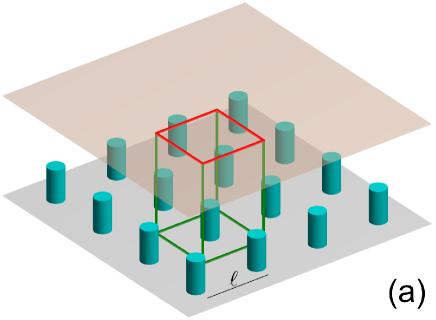
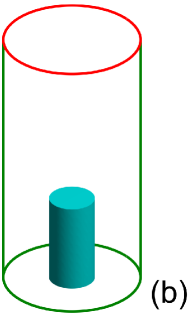
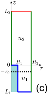
Figure 1: (a) A square-lattice array of cylindrical pillars (in light blue) on a support (in gray) and an upper plane (in pink) that is a source of particles. Periodicity of this domain allows one to treat diffusion in a single periodic cell around one pillar (shown by a rectangular parallelepiped). (b) A single pillar surrounded by an effective co-axial reflecting tube and capped by two parallel planes; (c) Planar ($xz$) projection of the three-dimensional domain. Red segment represents the source at the top, blue segments show the absorbing pillar and partially reactive base, and green segments indicate reflecting parts. Shadowed (light blue) region is the solid (inaccessible) interior of the cylindrical pillar. Black dotted line indicates the location $z=-z_{0}$ of the effective flat absorbing surface that receives the same total flux as the spiky coating (shown by blue segments). Here $R_{2}$ is the radius of the outer reflecting tube, $R_{1}$ is the radius of the absorbing pillar, $L_{1}$ is its height, and $L_{2}$ is the distance between the source and the top of the pillar (i.e., $L_{1}+L_{2}$ is the height of the whole system). Note that $R_{2}$ is related to the inter-pillar distance $\ell$, e.g., $R_{2}=\ell/\sqrt{\pi}$ for the square lattice. Restrictions of the solution to the lower subdomain (with $-L_{1}<z<0$) and to the upper subdomain (with $0<z<L_{2}$) are denoted by $u_{1}$ and $u_{2}$, respectively.

Mathematically the problem reduces to finding a solution to the Laplace equation in a domain with geometrically complex boundaries. The irregularity of the spiky profile makes the application of conventional perturbation methods difficult. For the two-dimensional profiles (comb-like structures) this difficulty can be overcome by means of conformal mapping Bernard_2001 ; Vandembroucq_1997 ; Skvortsov_2014 ; Grebenkov16 ; Hewett_2016 ; Skvortsov_2018 , which is inapplicable in three dimensions. One of the common methods for finding an approximate solution of such type of problems in any dimension consists in replacing the original irregular interface with an equivalent flat interface, which provides the same diffusive flux through the system but is amenable to analytical treatment Sapoval94 ; Sarkar_1995 ; Vandembroucq_1997 ; Grebenkov06 ; Skvortsov_2014 . Defining the equivalent interface for a particular geometry is not straightforward and is actually the main challenge of this approach (which is a variant of the effective medium approximation). For instance, Sarkar and Prosperetti Sarkar_1995 found an equivalent interface for a flat surface covered by a sparse configuration of hemispheroidal “bosses”. We emphasize that their method relies on regularity of the interface profile that prohibits its translation to the “spiky” limit (see Sec. III.2). Another example of an array of absorbing disks was discussed in Refs. Bruna15 ; Lindsay_2017 ; Bernoff18 ; Bernoff18b ; Paquin22 .

In this paper, we revisit the problem of steady-state diffusion towards a spiky coating, i.e., an array of absorbing spikes protruding from a flat base. We model this structure as an infinite square lattice of identical absorbing cylindrical pillars of radius $R_{1}$ and height $L_{1}$, in which the centers of the closest pillars are separated by the inter-pillar distance $\ell$ (Fig. 1(a)). We impose a constant concentration $c_{0}$ of particles at a distance $L_{2}$ above the pillars and aim at finding the total flux of particles onto each pillar, $J$, as a function of four geometric parameters of this model: $L_{1}$, $R_{1}$, $L_{2}$ and $\ell$. For this purpose, we follow the rationale by Keller and Stein Keller_1967 to reduce the original problem to that of diffusion inside a cylindrical tube towards a single co-axial pillar (Fig. 1(b)). The radius $R_{2}$ of the reflecting boundary of that tube can be directly related to the inter-pillar distance $\ell$ (see details below). After that, we derive the exact solution of the reduced problem and deduce the total flux as

$$J=\frac{\pi R_{2}^{2}Dc_{0}}{L_{2}+z_{0}}\,,$$ (1)

where $D$ is the diffusion coefficient, and $z_{0}$ is the offset parameter, which has the units of length and represents an aggregated effect of the inhomogeneous coating, incorporating the entire coating complexity (geometrical dimensions and non-uniform absorbing properties). This quantity, which depends only on the geometric parameters of the spiky coating and on the base reactivity, is the main interest of our study. Qualitatively, $-z_{0}$ can be understood as the location of an effective flat surface that produces the same far-away concentration profile as the coated surface Sarkar_1995 ; Vandembroucq_1997 ; Blyth_1993 ; Blyth_2003 ; Skvortsov_2014 :

$$c\approx c_{0}\frac{z+z_{0}}{L_{2}+z_{0}}\quad(z\geq-z_{0}),$$ (2)

where $c=c_{0}$ at $z=L_{2}$ and $c=0$ at $z=-z_{0}$. Alternatively, the effect of the coated surface can be represented by a flat partially reactive surface at $z=0$, with the effective reactivity $\kappa_{\rm eff}=D/z_{0}$ and the effective boundary condition $D\,\partial c/\partial z=\kappa_{\rm eff}\,c$ at $z=0$. The simple but universal form (1) of the total flux and the exact expression for $z_{0}$ are among the main results of the paper. Moreover, we will show that $z_{0}$ is (almost) independent of $L_{2}$ whenever $L_{2}\gg R_{2}$, but depends on two rescaled dimensions of the pillar: $\rho=R_{1}/R_{2}$ and $h=L_{1}/R_{2}$. We study the behavior of the total flux in different asymptotic regimes; in particular, we discover some new asymptotic relations and retrieve a few known ones such as, e.g., trapping by a disk in a tube ($h=0$). We also analyze the effect of the reactivity of the base by considering reflecting, absorbing and partially reactive cases.

The paper is organized as follows. In Sec. II, we formulate the mathematical problem, sketch the main steps of its exact solution, present an approximation solution and discuss some general properties. Section III explores the dependence of the total flux on the geometric parameters of the pillar. Section IV presents concluding remarks. The mathematical details of the derivation are re-delegated to Appendix.

II Main results

We consider point-like particles diffusing inside a three-dimensional layer between parallel planes at $z=-L_{1}$ and $z=L_{2}$. At steady state, the particle concentration $c$ obeys the three-dimensional Laplace equation

$$\Delta c=0.$$ (3)

The particle concentration at the top plane ($z=L_{2}$) is imposed to be constant: $c=c_{0}$. The bottom interface consists of an infinite square lattice of absorbing cylindrical pillars of height $L_{1}$ and radius $R_{1}$ protruding from a flat base at $z=-L_{1}$ (Fig. 1(a)). The surface of each pillar is absorbing ($c=0$), while the base can be absorbing, reflecting or partially reactive. To model spikes, one can set $R_{1}\ll L_{1}$ but we treat the general case.

Due to periodicity of the system in the $xy$ plane, one can consider the solution of Eq. (3) within one periodic cell around one pillar, i.e., within a cylinder $-L_{1}\leq z\leq L_{2}$ with the square cross-section $(-\ell/2,\ell/2)\times(-\ell/2,\ell/2)$ of the lattice cell, with $\ell$ being the distance between centers of two neighboring pillars (Fig. 1(a)). The symmetry of the periodic cell allows one to replace periodic boundary conditions on the square cross-section by reflecting (Neumann) boundary condition. In fact, eventual displacements between adjacent periodic cells do not affect the diffusive flux from the top plane to the absorbing coating. Moreover, we apply the rationale from Keller_1967 to replace the original periodic cell by a circular tube of radius $R_{2}$ with the reflecting boundary condition on its side wall (Fig. 1(b)). In this way, the solution of the original problem is approximated by that of the modified problem in a circular tube (see Bernoff18 ; Paquin22 and references therein for other methods to treat planar problems on Bravais lattices by preserving periodic conditions). The radius $R_{2}$ is chosen to get the same cross-sectional area, i.e., to preserve the volume of the cell; in the case of the square lattice, one gets

$$R_{2}=\frac{\ell}{\sqrt{\pi}}$$ (4)

(similar constructions can be made for other regular lattices, e.g., a hexagonal lattice).

From now on, we focus on steady-state diffusion inside a cylindrical domain $\Omega$ of radius $R_{2}$, capped by parallel planes at $z=-L_{1}$ and $z=L_{2}$, which contains another co-axial cylinder of radius $R_{1}$ (an absorbing pillar), capped by parallel planes at $z=-L_{1}$ and $z=0$, as shown on Fig. 1(b). We search for the harmonic function $u(r,z)$ satisfying the following boundary value problem in cylindrical coordinates $(r,z,\phi)$:

$$\Delta u=0\quad\textrm{in}~{}\Omega,$$ (5a)

$$u(r,L_{2})=1\quad(r<R_{2}),$$ (5b)

$$u(r,0)=0\quad(r<R_{1}),$$ (5c)

$$u(R_{1},z)=0\quad(-L_{1}<z<0),$$ (5d)

$$(\partial_{r}u(r,z))_{r=R_{2}}=0\quad(-L_{1}<z<L_{2}),$$ (5e)

$$\bigl{[}D\partial_{z}u(r,z)+\kappa_{b}u(r,z)\bigr{]}_{z=-L_{1}}=0\quad(R_{1}<r<R_{2}),$$ (5f)

where $\Delta=\partial_{r}^{2}+(1/r)\partial_{r}+\partial_{z}^{2}$ is the Laplace operator in cylindrical coordinates (without the angular part), $D$ is the diffusion coefficient, and $\kappa_{b}$ is the reactivity of the base, which can take any value between $\kappa_{b}=0$ for a reflecting base and $\kappa_{b}=\infty$ for an absorbing base. Here, Eq. (5b) sets the homogeneous source of particles at the top boundary, Eqs. (5c, 5d) incorporate the absorbing pillar, Eq. (5e) describes the reflecting outer cylindrical surface, and Eq. (5f) accounts for partial reactivity of the bottom base. The rotation invariance of this problem implies that $u$ does not depend on the angle $\phi$, which therefore will be omitted in what follows. Multiplication of $u(r,z)$ by $c_{0}$ yields the concentration of particles inside the domain, while

$$J=c_{0}\int\limits_{0}^{R_{2}}dr\,r\,\bigl{(}D\partial_{z}u(r,z)\bigr{)}_{z=L_{2}}$$ (6)

is the total diffusive flux of particles that enter into the domain from the top disk. Due to the conservation of particles inside the domain, this is precisely the diffusive flux of particles onto the absorbing boundary (i.e., the pillar and the reactive base if $\kappa_{b}>0$). We aim at finding exact and approximate solutions of the problem (5) and then analyze the dependence of the total flux $J$ on the geometric parameters $L_{1}$, $R_{1}$, $L_{2}$, $R_{2}$ for different $\kappa_{b}$.

Note that $u(r,z)$ can be interpreted as the splitting probability: if the particle started from a point $(r,z)$, then $u(r,z)$ is the probability of its first arrival onto the top disk before hitting the pillar (or reacting on the bottom base if $\kappa_{b}>0$). This interpretation opens a way to access $u(r,z)$ and the total flux by Monte Carlo simulations, see Appendix A.6 for details.

II.1 Exact solution

The exact solution of Eq. (5) can be found by a mode matching method (see Delitsyn18 ; Grebenkov18 ; Delitsyn22 and references therein). In a nutshell, one can represent a harmonic function $u(r,z)$ in the subdomains $-L_{1}<z<0$ and $0<z<L_{2}$ as two series involving appropriate Bessel functions. Matching these two representations at $z=0$ yields an infinite system of linear algebraic equations on the unknown coefficients of these series. The last step entails solving this system of equations by truncation and numerical inversion of a finite-size matrix with explicitly known elements. Despite the need for the numerical inversion of a matrix, the resulting solution yields an analytical dependence of $u(r,z)$ on $r$ and $z$, offers an efficient tool for its numerical computation, and allows for asymptotic analysis. Even though the exact solution is one of the main results of this paper, we re-delegate the details of its derivation to Appendix A. In particular, the total diffusive flux $J$ is given by Eq. (59) that we rewrite with the aid of Eq. (61) in the form (1). The offset parameter $z_{0}$ depends on the reactivity $\kappa_{b}$ of the base and on the geometric parameters $R_{1}$, $L_{1}$, $L_{2}$, $R_{2}$ in a sophisticated way via the exact relation (62). This dependence is the main object of our study.

II.2 Diagonal approximation

The exact relation (62) determining the offset parameter $z_{0}$ requires the inversion of the infinite-dimensional matrix $I+W^{\prime}$, whose elements are known explicitly (see Appendix A). As a consequence, the dependence of $z_{0}$ on the geometric parameters remains hidden through this inversion, which has to be done numerically. Motivated by the ideas of Refs. Benichou11 ; Calandre14 ; Benichou15 , we conducted a thorough inspection of numerical results for different configurations of parameters. This revealed that the diagonal elements of the matrix $W^{\prime}$ are generally dominant as compared to non-diagonal elements. This let us to propose a diagonal approximation, in which the matrix $W^{\prime}$ is replaced by a diagonal matrix formed by the diagonal elements of $W^{\prime}$. In other words, all non-diagonal elements of this matrix are set to $0$ that yields

$$J_{\rm app}=\frac{\pi R_{2}^{2}Dc_{0}}{L_{2}+z_{0,\rm app}}\,,$$ (7)

with

$$z_{0,\rm app}=L_{2}\biggl{(}W_{0,0}-\sum\limits_{k=1}^{\infty}\frac{W_{0,k}W_{k,0}}{1+W_{k,k}}\biggr{)},$$ (8)

where the elements of the matrix $W$ (or $W^{\prime}$) are given explicitly by Eq. (55). Even though the dependence of the offset $z_{0,\rm app}$ on the geometric parameters may still be complicated, it is fully explicit within this approximation, as there is no matrix inversion anymore. As discussed in the following, this approximation gives very accurate results for a broad range of geometric parameters.

II.3 General properties of the rescaled offset

We aim at understanding how the offset parameter $z_{0}$ (and thus the total flux $J$) depends on four dimensionless parameters:

$$\rho=\frac{R_{1}}{R_{2}}\,,\quad h=\frac{L_{1}}{R_{2}}\,,\quad H=\frac{L_{2}}{R_{2}}\,,\quad\kappa=\frac{\kappa_{b}}{D}R_{2}.$$ (9)

By construction, the rescaled radius $\rho$ of the pillar ranges from $0$ to $1$, whereas its rescaled height $h$ can take any positive value: $h\geq 0$.

At the end of Appendix A.2, we show that the offset $z_{0}$ does not almost depend on $L_{2}$ whenever $L_{2}\gg R_{2}$, i.e., when the source of particles is much further than the inter-pillar distance, which is a typical setting for most applications. This is an expected behavior because $z_{0}$ (or, equivalently, $\kappa_{\rm eff}=D/z_{0}$) is the intrinsic “material” property of the spiky coating (like an impedance), so it is a function of $R_{1}$, $R_{2}$, $L_{1}$, and $\kappa_{b}/D$, but it should be independent of $L_{2}$. In the following, we impose the condition $L_{2}\gg R_{2}$ to eliminate the geometric parameter $L_{2}$ from the analysis and rewrite Eq. (1) as

$$J=\frac{\pi R_{2}^{2}Dc_{0}}{L_{2}+R_{2}\zeta_{\kappa}(\rho,h)}\,,$$ (10)

where

$$\zeta_{\kappa}(\rho,h)=\lim\limits_{L_{2}\to\infty}\frac{z_{0}}{R_{2}}$$ (11)

is the dimensionless offset in the limit $L_{2}\to\infty$. One sees that the total flux $J$ depends on $L_{2}$ in a trivial way, i.e., via $L_{2}$ standing in the denominator of Eq. (10). In turn, the rescaled offset aggregates the dependences on other parameters.

Let us first look at the function $\zeta_{\kappa}(\rho,h)$ in the limit $\rho=1$ when the pillar fills the whole tube for $-L_{1}<z<0$, and one simply gets one-dimensional diffusion from the top disk to the bottom absorbing disk, with the elementary solution $u_{0}(r,z)=z/L_{2}$ and the total flux

$$J_{\rm max}=\frac{\pi R_{2}^{2}Dc_{0}}{L_{2}}\,,$$ (12)

i.e.,

$$\zeta_{\kappa}(1,h)=0.$$ (13)

In this trivial limit, there is no base (other than the pillar itself) so that the flux does not depend neither on $\kappa$, nor on $h$.

In turn, if $\rho<1$, thinning of the pillar removes an easily accessible part of the absorbing disk at $z=0$ with $R_{1}<r<R_{2}$ and thus diminishes the diffusive flux. As a consequence, the configuration with $\rho=1$ yielded the maximal flux, i.e.,

$$1\geq\frac{J}{J_{\rm max}}=\frac{1}{1+\zeta_{\kappa}(\rho,h)\frac{R_{2}}{L_{2}}}$$ (14)

so that

$$\zeta_{\kappa}(\rho,h)\geq 0$$ (15)

for any set of parameters $\rho$, $h$ and $\kappa$. In other words, the offset is always positive. This observation may sound counter-intuitive because the total absorbing surface of the pillar, $\pi R_{1}^{2}+2\pi R_{1}L_{1}$, can dramatically increase due to its cylindrical part (the second term). However, this cylindrical part is less accessible to Brownian particles due to the so-called diffusional screening Traytak92 ; Felici03 ; McDonald03 ; McDonald04 ; Traytak07 ; Andrade07 ; Traytak18 by the top disk (or by the singularity in concentration profile when the diameter of the top disk tends to zero) so that the gain in the total absorbing surface is compensated by its lower accessibility Grebenkov05 ; Grebenkov05b .

To get more insights into this property, one can rely on an equivalent electrostatic problem of finding the electric current $J$ through a conducting medium between two metallic electrodes (at the top and the bottom), to which a voltage $c_{0}$ is applied Liu85 ; Sapoval94 . In the case of two flat parallel electrodes at $z=L_{2}$ and $z=0$, one has $z_{0}=0$ and Eq. (1) yields the overall resistance, $\mathcal{R}_{0}=c_{0}/J=L_{2}/(D\pi R_{2}^{2})$, where $1/D$ can be interpreted as the resistivity of the medium, while $L_{2}$ and $\pi R_{2}^{2}$ are the length and the cross-sectional area of such a cylindrical wire. In turn, if the conducting medium lies between the top flat electrode and the bottom spiky electrode, the inclusion of the bottom part with $z<0$ adds more resistive material between two electrodes and can only increase the overall resistance and thus decrease the current, in agreement with the inequality (14). In this electrostatic analogy, it is clear that an increased area of the bottom electrode does not matter. In this light, Eq. (1) can also be written as

$$J=\frac{c_{0}}{\mathcal{R}_{0}+\mathcal{R}_{b}}\,,\qquad\mathcal{R}_{b}=\frac{z_{0}}{\pi R_{2}^{2}D}\,,$$ (16)

where $\mathcal{R}_{b}$ can be interpreted as the resistance of the lower layer $-L_{1}<z<0$, which is connected in series to the resistance $\mathcal{R}_{0}$ of the upper (flat) layer $0<z<L_{2}$. This representation provides yet another revealing insight onto $z_{0}$ as the length of an effective “wire” of the cross-sectional area $\pi R_{2}^{2}$ and resistivity $1/D$. Even though this electrostatic analogy was formulated for the absorbing base, the underlying arguments can be extended to the reflecting base as well.

In order to quantify the diffusional screening, in Appendix A.3 we computed the flux of particles onto the top of the pillar, $J_{\rm top}$, which determines the fraction of particles, $J_{\rm top}/J$, captured there. Moreover, when the base is not reflecting and can thus capture some particles, it is instructive to get the fraction of particles absorbed by the base. For this purpose, we also computed the flux onto the base $J_{\rm base}$. We will discuss the behavior of these two quantities in the next section.

It is worth noting that some references reported negative values of $z_{0}$ (see, e.g., Skvortsov_2019 ). However, this is a consequence of convention that was used in that references to write the total flux as $J=\pi R_{2}^{2}Dc_{0}/(L+z^{\prime}_{0})$, where $L=L_{1}+L_{2}$ is the total distance between the top disk at $z=L_{2}$ and the bottom base at $z=-L_{1}$, and prime distinguishes the new offset $z^{\prime}_{0}$ from our parameter $z_{0}$. Evidently, one has $z^{\prime}_{0}=z_{0}-L_{1}$, i.e., $z^{\prime}_{0}$ can take positive or negative values depending on whether $z_{0}$ is larger or smaller than $L_{1}$. We keep using our convention, which follows from the exact solution of the problem.

Finally, we stress that the effective flat absorbing surface at $z=-z_{0}$ may lie below the bottom base at $z=-L_{1}$, i.e., outside the considered domain. If one needs to avoid such locations, the lowest location can be limited to the base level $z=-L_{1}$, but one would have to replace the absorbing surface by partially reactive surface, with the effective reactivity $\kappa^{\prime}_{\rm eff}$ such that $z_{0}=L_{1}+D/\kappa^{\prime}_{\rm eff}$. In other words, there are infinitely many effective partially reactive surfaces at different locations, which yield the same $z_{0}$ and thus the same total flux (see also Martin_2022b ).

III Discussion

In this section, we investigate the dependence of the total flux through the system on the geometric parameters in several asymptotic regimes. We start with a pillar on the reflecting base and then consider the absorbing base.

III.1 Reflecting base

When the base is reflecting ($\kappa=0$), the particles can only be absorbed on the pillar. Expectedly, the flux diminishes as the absorbing pillar gets smaller, i.e., when either $\rho$ or $h$ decreases (or both). Note that the flux vanishes in the limit $\rho\to 0$ for any fixed $h$ because the pillar shrinks to a one-dimensional interval (a needle), which is “invisible” for Brownian motion Morters . In turn, the flux remains strictly positive in the limit $h\to 0$ for any fixed $\rho>0$ when the pillar transforms into a planar absorbing disk, which remains accessible for Brownian motion. Panel (a) of Fig. 2 illustrates these properties of the total flux, while the panel (b) presents the corresponding offset $\zeta_{0}(\rho,h)$. As stated earlier, the ratio $J/J_{\rm max}$ is equal to $1$ for $\rho=1$ and any $h$, and it remains below $1$ for other parameters. Moreover, one observes that $J$ and $\zeta_{0}(\rho,h)$ are monotonous functions of $\rho$ and $h$. Even though this observation is intuitively expected, its rigorous demonstration presents an interesting perspective for future work.

Let us now inspect the panel (c) of Fig. 2, which shows the absolute value of the relative error, $|J_{\rm app}/J-1|$, of the diagonal approximation of the flux $J_{\rm app}$ given by Eq. (7). When the pillar is long enough (say, $h\gtrsim 1$), the relative error is below $1\%$, whatever the rescaled radius $\rho$ is. As the pillar gets shorter, the relative error increases, even though the approximation remains applicable when $\rho$ is small enough (e.g., the relative error is around $10\%$ when $\rho\lesssim 0.1$). The worst case corresponds to short wide pillars (i.e., when the pillar is close to a disk). In this particular case, one can employ another approximation, as discussed below. Overall, we conclude that the diagonal approximation (7) yields very accurate results for a broad range of geometric parameters. At the same time, the dependence of the approximate offset $z_{0,\rm app}$ in Eq. (8) on the geometric parameters yet requires further analysis. To shed light on it, we explore several asymptotic regimes.

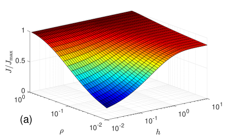
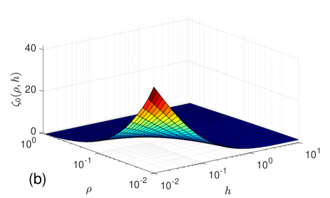
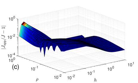
Figure 2: (a) The total flux $J$ (rescaled by $J_{\rm max}=\pi R_{2}^{2}Dc_{0}/L_{2}$) as a function of $\rho=R_{1}/R_{2}$ and $h=L_{1}/R_{2}$ for the reflecting base ($\kappa=0$). The function $J$ was computed from Eq. (59), in which the coefficient $c_{0,2}$ was obtained by inverting numerically the matrix $I+W$ truncated to the size $N\times N$ with $N=50$, see Appendix A for details. We used $L_{2}/R_{2}=10$. (b) The corresponding dimensionless offset $\zeta_{0}(\rho,h)$ as a function of $\rho=R_{1}/R_{2}$ and $h=L_{1}/R_{2}$. (c) The absolute value of the relative error, $|J_{\rm app}/J-1|$, of the diagonal approximation $J_{\rm app}$ from Eq. (7).

Disk-like pillar

We start by considering the limit $L_{1}=0$ when the pillar shrinks to an absorbing disk of radius $R_{1}$ located on the reflecting base at $z=0$. This problem was first studied by Fock Fock41 and later by other researchers (see Skvorstov21 ; Grebenkov22c and references therein). In particular, an approximate analytical expression for the steady-state diffusive flux has been derived for a tube that contains a perpendicular barrier with a circular hole Skvorstov21 . This setting is identical to the case of a disk-like pillar on the reflecting base, so that we should get

$$\zeta_{0}(\rho,0)\approx\frac{\pi}{4\rho}M(\rho),$$ (17)

where $M(\rho)$ is the Fock function, which can be approximated as Skvorstov21 ; Grebenkov22c (see also Leppington_1972 ):

$$M(\rho)=\frac{(1-\rho^{2})^{2}}{1+1.37\rho-0.37\rho^{4}}\,.$$ (18)

Figure 3 confirms the remarkable accuracy of the total flux given by Eq. (1) with $z_{0}=R_{2}\zeta_{0}(\rho,0)$ from Eq. (17) over the whole range of radii $\rho$. Note that a simpler approximation $\zeta_{0}(\rho,0)\approx\pi/(4\rho)$ (i.e., without the Fock function) is still accurate at small $\rho$ but exhibits moderate deviations at larger $\rho$.

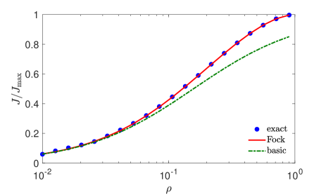
Figure 3: The total flux $J$ (rescaled by $J_{\rm max}=\pi R_{2}^{2}c_{0}D/L_{2}$) as a function of $\rho=R_{1}/R_{2}$, at $L_{2}/R_{2}=5$, $L_{1}=0$ and $\kappa=0$ (an absorbing disk on the reflecting base). Filled circles present the exact solution obtained with the truncation order $N=50$, while solid line shows the flux from Eq. (1), with $z_{0}/R_{2}=\zeta_{0}(\rho,0)$ given by Eq. (17). Dashed line presents the flux with $\zeta_{0}(\rho,0)\approx\pi/(4\rho)$, i.e., without the Fock function $M(\rho)$.

Capacitance approximation

Before dwelling into the asymptotic analysis of the exact solution, it is instructive to discuss the capacitance approximation, which is commonly used for estimating the steady-state flux and other related quantities Redner_2001 ; Krapivsky ; Hughes ; Zhou94 ; Grebenkov20 . When both dimensions of the pillar ($R_{1}$ and $L_{1}$) are much smaller than $R_{2}$ and $L_{2}$, it is tempting to treat the outer reflecting cylindrical surface and the upper absorbing disk as being at infinity, i.e., to consider a single absorbing pillar in the infinite upper half-space (above the reflecting base). In this case, the total flux is determined by the capacitance ${\mathcal{C}}$ of the absorbing pillar as $J_{\infty}=c_{0}D{\mathcal{C}}$, where $c_{0}$ is the concentration kept at infinity (here we employ the definition, according to which the capacitance of a sphere of radius $R$ is $4\pi R$). The mirror reflection of the pillar with respect to the reflecting base allows one to express ${\mathcal{C}}$ as half of the capacitance ${\mathcal{C}}_{0}$ of the twice longer pillar in the whole space ${\mathbb{R}}^{3}$. The latter is known exactly Sandua_2013 and thus yields

$${\mathcal{C}}=\frac{1}{2}{\mathcal{C}}_{0}=2\pi R_{1}\frac{1+(L_{1}/R_{1})^{2}}{\frac{\pi}{2}+\frac{L_{1}}{R_{1}}\ln\frac{L_{1}}{R_{1}}}$$ (19)

(note that former expressions for the capacitance ${\mathcal{C}}_{0}$ were given in terms of a series expansion in powers of $1/\ln(L_{1}/R_{1})$, see e.g., Jackson00 ; Chang70 ; Riba18 and references therein). As $L_{1}\to 0$, one retrieves half of the capacitance $8R_{1}$ of an absorbing disk in ${\mathbb{R}}^{3}$. The factor $1/2$ in the above relation corrects the twice larger total flux, which was artificially doubled by mirror reflection with respect to the reflecting base. The total flux onto the pillar can thus be approximated as

$$J_{\infty}=c_{0}D{\mathcal{C}}=2\pi c_{0}DR_{1}\frac{1+(L_{1}/R_{1})^{2}}{\frac{\pi}{2}+\frac{L_{1}}{R_{1}}\ln\frac{L_{1}}{R_{1}}}\,.$$ (20)

Strictly speaking, this approximation is incompatible with our exact form (1), which is valid for any finite $R_{2}$ and $L_{2}$. In fact, when $R_{2}$ is fixed and $L_{2}$ increases, Eq. (1) implies that $J\propto 1/L_{2}$, i.e., the total flux vanishes as $L_{2}\to\infty$, in contradiction with Eq. (20). In other words, the approximation (20) might only be applicable in the double limit when $R_{2}\to\infty$ and $L_{2}\to\infty$ simultaneously. However, there are infinitely many ways to relate $R_{2}$ and $L_{2}$ in order to undertake this double limit. While the detailed inspection of this mathematical issue is beyond the scope of the paper, we mention one possible way.

One can rely on earlier works (see, e.g., Berezhkovskii_2004 ; Berezhkovskii07 and references therein) that expressed the effective reactivity of an absorber inside a reflecting tube as $\kappa_{\rm eff}\approx D{\mathcal{C}}/{\mathcal{A}}$, where ${\mathcal{A}}=\pi R_{2}^{2}$ is the surface area of the tube cross-section. As a consequence, the total flux is given by Eq. (1), with

$$z_{0}=\frac{D}{\kappa_{\rm eff}}\approx\frac{\pi R_{2}^{2}}{{\mathcal{C}}}\,.$$ (21)

Substituting Eq. (19), we get

$$\zeta_{0}(\rho,h)\approx\biggl{(}2\rho\,\frac{1+(h/\rho)^{2}}{\frac{\pi}{2}+\frac{h}{\rho}\ln\frac{h}{\rho}}\biggr{)}^{-1}$$ (22)

for $\rho\ll 1$ and $h\ll 1$. In the double limit $L_{2}\to\infty$ and $R_{2}\to\infty$ with $H=L_{2}/R_{2}$ being fixed, the total flux tends to the limit $J_{\infty}$ from Eq. (20) for the pillar in the upper half-space, which is independent of $H$, as expected. However, the quality of this approximation for finite $L_{2}$ and $R_{2}$ depends on $H$. We stress that the limit $R_{2}\to\infty$ is singular; in particular, the spectrum of the Laplace operator in the unbounded domain with $R_{2}=\infty$ is not discrete anymore, and other mathematical tools are required to analyze the asymptotic behavior. For this reason, the above discussion remains speculative from the mathematical point of view.

Figure 4 illustrates the asymptotic behavior by showing how the total flux increases when both $R_{2}$ and $L_{2}$ increase with $H=L_{2}/R_{2}$ being fixed. In this double limit, two opposite effects seem to almost compensate each other: on the one hand, an increase of $L_{2}$ diminishes the flux (as the source is getting further from the absorbing pillar); on the other hand, an increase of $R_{2}$ enlarges the area of the source (the top disk) and thus the flux. Even though the capacitance approximation (22) shows a similar trend, it is not accurate.

We expect that the capacitance approximation may be deduced from the asymptotic analysis of $\zeta_{0}(\rho,h)$ as both $\rho$ and $h$ go to $0$, with $h/\rho=L_{1}/R_{1}$ being fixed. However, even the numerical computation of the total flux at very large $R_{2}$ is difficult because larger and larger truncation orders are needed as $R_{2}$ increases. Further theoretical analysis of this limit presents therefore an interesting perspective for future research.

At the same time, we recall that very large $R_{2}$ corresponds to an arrangement of very distant short pillars, which is not a common setting for applications. In the rest of the text, we keep $R_{2}$ fixed and consider $L_{2}\gg R_{2}$, as stated earlier.

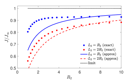
Figure 4: The total flux $J$ (rescaled by $J_{\infty}$) as a function of $R_{2}$ for $R_{1}=0.1$, $L_{1}=0.5$, and two choices $L_{2}=R_{2}$ (circles) and $L_{2}=2R_{2}$ (squares). Symbols present the exact solutions with the truncation order $N=50$. Lines show Eq. (1) with $z_{0}=R_{2}\zeta_{0}(\rho,h)$ given by the approximation (22). Dotted horizontal line indicates the limit determined by the flux $J_{\infty}$ from Eq. (20), which corresponds to the double limit $R_{2}\to\infty$ and $L_{2}\to\infty$.

Thin pillar approximation

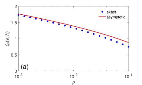
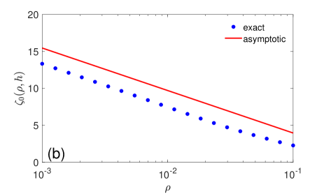
Figure 5: The dimensionless offset $\zeta_{0}(\rho,h)$ as a function of $\rho$ for $h=5$ (a) and $h=0.2$ (b) for the reflecting base ($\kappa=0$). Filled circles present this function deduced from for the total flux, which was obtained by truncation at $N=20$. Solid line shows the asymptotic relation (25).

Let us now look at the setting $\rho\ll 1$, which corresponds to thin pillars, which are well-separated from each other (i.e. $R_{1}\ll\ell=\sqrt{\pi}R_{2}$). In this limit, the widths $R_{2}$ and $R_{2}-R_{1}$ of the upper and lower subdomains are almost equal (see Fig. 1(c)), and they differ essentially by the boundary condition on the left edge. The absorbing boundary in the lower subdomain can be treated via standard “strong perturbation” asymptotic tools Mazya85 ; Ward93 . Re-delegating the derivation steps to Appendix A.4, we discuss here the derived asymptotic approximation:

$$\zeta_{\kappa}(\rho,h)\approx\frac{1}{\alpha_{0,1}}\,\frac{\alpha_{0,1}+\kappa\tanh(\alpha_{0,1}h)}{\kappa+\alpha_{0,1}\tanh(\alpha_{0,1}h)}\quad(\rho\to 0),$$ (23)

where

$$\alpha_{0,1}\approx\frac{\sqrt{2}}{\sqrt{\ln(1/\rho)-3/4}}\qquad(\rho\to 0).$$ (24)

For the reflecting base ($\kappa=0$), one gets an even simpler relation:

$$\zeta_{0}(\rho,h)\approx\frac{\mathrm{ctanh}(\alpha_{0,1}h)}{\alpha_{0,1}}\quad(\rho\to 0),$$ (25)

i.e., the offset logarithmically diverges as $\rho\to 0$, implying that the total flux $J$ vanishes in this limit, as expected. However, as the offset $z_{0}\approx R_{2}\zeta_{0}(\rho,h)$ is added to a large distance $L_{2}$, this decay is extremely slow, especially for large $h$, as one can see on Fig. 2(a). We stress that the height of the pillar affects this speed:

(i) if $h\gg 1$ (or even $h=\infty$), the argument $\alpha_{0,1}h$ can be large even for extremely small $\rho$, and the numerator of Eq. (25) can be replaced by $1$, yielding

$$\zeta_{0}(\rho,h)\approx\frac{\sqrt{\ln(1/\rho)-3/4}}{\sqrt{2}}\quad(\rho\to 0,~{}h\gg 1),$$ (26)

independently of the height $h$. Qualitatively, a very large height of the pillar almost compensates for its vanishing radius.

(ii) In contrast, if $0<h\ll 1$, one gets

$$\zeta_{0}(\rho,h)\approx\frac{\ln(1/\rho)-3/4}{2h}\quad(\rho\to 0,~{}0<h\ll 1).$$ (27)

In this regime, the value of $\zeta_{0}(\rho,h)$ is also affected by the height $h$: as the pillar is getting shorter, $\zeta_{0}(\rho,h)$ increases, as expected. Note that the case $h=0$ (an absorbing disk) should be treated separately, as we did earlier. Comparing the asymptotic expressions (17, 27), one sees that the order of the limits, $\rho\to 0$ and $h\to 0$, is important. This is a manifestation of the absorber anisotropy, which was earlier reported for other geometric settings (see, e.g., Grebenkov_2017 ; Chaigneau22 ).

Figure 5 illustrates the behavior of the offset $\zeta_{0}(\rho,h)$ and its asymptotic approximation (25) for a long pillar ($h=5$) and a short pillar ($h=0.2$). In both cases, Eq. (25) captures correctly the leading-order, divergent behavior. In turn, one can observe a nearly constant deviation (i.e., a shift between two curves along the vertical axis), especially for the shorter pillar. This deviation is caused by the next-order corrections which seem to be of the order $O(1)$. Further investigation of this asymptotic behavior presents an interesting perspective of this work.

Diffusional screening by the top of the pillar

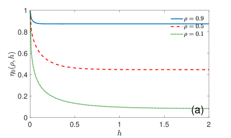
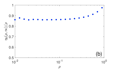
Figure 6: (a) The fraction $\eta_{0}(\rho,h)$ of particles absorbed on the top of the pillar on the reflecting base ($\kappa=0$), as a function of the pillar height $h=L_{1}/R_{1}$, for three values of $\rho=R_{1}/R_{2}$ (see the legend). This fraction was obtained from Eq. (66) with $L_{2}/R_{2}=5$ and $N=50$. (b) The fraction $\eta_{0}(\rho,\infty)$ divided by $\rho$.

We complete this section by quantifying the diffusional screening effect. In Appendix A.3, we calculated the flux on the top of the pillar, $J_{\rm top}$, and deduced the fraction of particles absorbed there, $\eta_{\kappa}(\rho,h)$, as the limit of the ratio $J_{\rm top}/J$ as $L_{2}\to\infty$, see Eq. (66).

Figure 6(a) illustrates the dependence of the ratio $\eta_{0}(\rho,h)$ on the geometric parameters of the pillar: rescaled height $h$ and radius $\rho$. In the limit $h=0$, there is no cylindrical part of the pillar, and the whole flux is absorbed on the top: $\eta_{0}(\rho,0)=1$. As $h$ increases, the cylindrical part of the pillar starts to absorb the particles, and the ratio $\eta_{0}(\rho,h)$ decreases to a strictly positive limit $\eta_{0}(\rho,\infty)$ as $h\to\infty$. This limiting value depends on the radius of the pillar. As $\rho$ stands in Eq. (66) as a prefactor, we plot $\eta_{0}(\rho,\infty)/\rho$ on Fig. 6(b). One can see that this function grows from $0.86$ to $1$. It is worth noting, however, that an accurate computation of $\eta_{0}(\rho,\infty)$ was difficult due to a slow convergence of the series in Eq. (65). To overcome this difficulty, we computed the ratio $J_{\rm top}/J$ from Eq. (65) by truncating matrices at orders $N=100,200,\ldots,1000$ and then performed a linear regression of the obtained values versus $1/\sqrt{N}$ to extrapolate the ratio to the limit $N\to\infty$. Despite this refined analysis, one can notice minor fluctuations of $\eta_{0}(\rho,\infty)/\rho$ at small $\rho$. In particular, we cannot rigorously state whether this ratio converges a strictly positive constant around $0.86$ (as it seems to be the case according to Fig. 6(b)), or exhibits an extremely slow decay as $\rho\to 0$. Further mathematical and numerical analysis of this issue presents an interesting perspective.

III.2 Absorbing base

Let us switch to the analysis of the absorbing pillar on the absorbing base ($\kappa_{b}=\infty$). As both the pillar and the base can now absorb particles, the dependence of the total flux on the geometric parameters is quite different. Figure 7(a) illustrates this dependence, while the panel (b) presents the corresponding offset parameter $\zeta_{\infty}(\rho,h)$. In addition to the trivial limit (13) at $\rho=1$, one also has $\zeta_{\infty}(\rho,0)=0$. In fact, if the pillar shrinks to an absorbing disk lying on the absorbing base, one simply deals with a whole flat absorbing surface at $z=0$. As a consequence, the only nontrivial behavior emerges for small $\rho$ and large $h$. Moreover, even in this region, the offset parameter $\zeta_{\infty}(\rho,h)$ remains small as compared to $L_{2}/R_{2}\gg 1$, yielding only a moderate decrease of the total flux. This is in sharp contrast to the behavior in the case of the reflecting base shown in Fig. 2. We also stress that the relative error of the approximate flux from Eq. (7) is below $1\%$ for the whole considered range of parameters $\rho$ and $h$. In other words, the diagonal approximation is remarkably accurate in the case of the absorbing base.

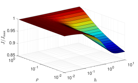
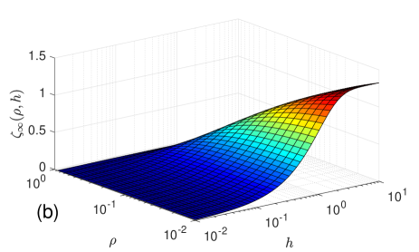
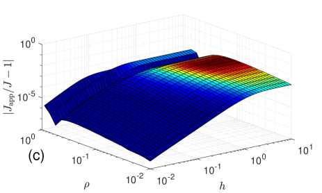
Figure 7: (a) The total flux $J$ (rescaled by $J_{\rm max}=\pi R_{2}^{2}Dc_{0}/L_{2}$) as a function of $\rho=R_{1}/R_{2}$ and $h=L_{1}/R_{2}$ for the absorbing base ($\kappa=\infty$). The function $J$ was computed from Eq. (59), in which the coefficient $c_{0,2}$ was obtained by inverting numerically the matrix $I+W$ truncated to the size $N\times N$ with $N=50$, see Appendix A for details. We used $L_{2}/R_{2}=10$. (b) The corresponding dimensionless offset $\zeta_{\infty}(\rho,h)$ as a function of $\rho=R_{1}/R_{2}$ and $h=L_{1}/R_{2}$. (c) The absolute value of the relative error, $|J_{\rm app}/J-1|$, of the diagonal approximation $J_{\rm app}$ from Eq. (7).

Thin pillar approximation

When the pillar is thin ($\rho\ll 1$), one can use again Eq. (23), which reads for the absorbing base as

$$\zeta_{\infty}(\rho,h)\approx\frac{\tanh(\alpha_{0,1}h)}{\alpha_{0,1}}\,.$$ (28)

One can distinguish two cases:
(i) If $h=\infty$, one has

$$\zeta_{\infty}(\rho,h)\approx\frac{1}{\alpha_{0,1}}\approx\frac{\sqrt{\ln(1/\rho)-3/4}}{\sqrt{2}}\,,$$ (29)

which slowly diverges as $\rho\to 0$. Expectedly, as the base is infinitely far away, its reactivity does not matter, and we retrieve the behavior given by Eq. (26) for the reflecting base.
(ii) If $h<\infty$, the expansion of the hyperbolic tangent yields $\zeta_{\infty}(\rho,h)\approx h$, i.e., there is no divergence, and the offset reaches a finite limit equal to $h$. In fact, even if the pillar has vanished, the particle can react on the base, and the offset increases (i.e., the total flux decreases) when the base is getting further from the source, as expected. Note that the same behavior also holds for a partially reactive base ($0<\kappa<\infty$).

Diffusional screening

As the top of the pillar is the most exposed to the source, it may absorb a considerable fraction of particles and thus screen the cylindrical part of the pillar and the base. Panel (a) of Fig. 8 presents the fraction $\eta_{\infty}(\rho,h)$ of particles absorbed on the top of the pillar. When $h=0$, the disk-like pillar lies on the absorbing base and therefore absorbs the fraction of particles that is given by its relative surface area, i.e., $\eta_{\infty}(\rho,0)=\rho^{2}$. As the pillar’s height increases, one might expect that this fraction would diminish, as the total area of the absorbing surface increases due to the emergence of the cylindrical part of the pillar. However, one sees the opposite trend, i.e., $\eta_{\infty}(\rho,h)$ actually increases with $h$. We already discussed in Sec. II.3 that the cylindrical surface of the pillar, as well as the absorbing base itself, are getting less accessible due to diffusional screening when $h$ increases. Panel (a) re-confirms this behavior by showing a monotonous growth of $\eta_{\infty}(\rho,h)$ with $h$. In the limit $h\to\infty$, $\eta_{\infty}(\rho,h)$ approaches a finite value, which is independent of the base reactivity $\kappa$. Its dependence on $\rho$ was illustrated on Fig. 6(b).

As the base is absorbing, it is instructive to quantify the fraction of particles absorbed on that base, i.e., $J_{\rm base}/J$. The limit $\eta^{\prime}_{\infty}(\rho,h)$ of this fraction as $L_{2}\to\infty$ is shown on panel (b) of Fig. 8. At $h=0$, one simply has $\eta^{\prime}_{\infty}(\rho,0)=1-\rho^{2}$. When $h$ increases, the base is getting further from the source so that this fraction should decrease. According to our exact expression (68), this fraction vanishes exponentially fast, i.e., $\eta^{\prime}_{\infty}(\rho,h)\propto e^{-\alpha_{0,1}h}$ as $h\to\infty$. In turn, the rate of this exponential decay, given by $\alpha_{0,1}$ from Eq. (40), slowly vanishes as $\rho\to 0$ according to Eq. (24). In fact, as the pillar gets thinner, it has a lower capacity to capture particles, which have therefore higher chances to reach a remote absorbing base.

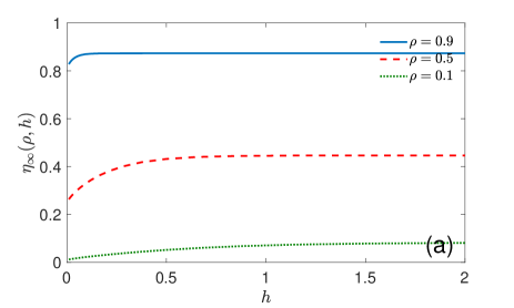
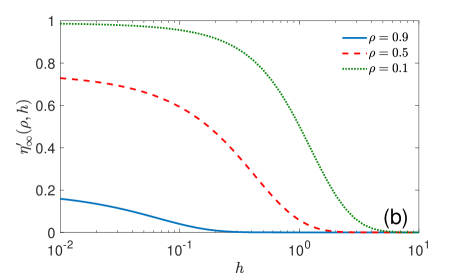
Figure 8: (a) The fraction $\eta_{\infty}(\rho,h)$ of particles absorbed on the top of the pillar on the absorbing base ($\kappa=\infty$), as a function of the pillar height $h=L_{1}/R_{1}$, for three values of $\rho=R_{1}/R_{2}$ (see the legend). This fraction was obtained from Eq. (66) with $L_{2}/R_{2}=5$ and $N=50$. (b) The fraction $\eta^{\prime}_{\infty}(\rho,h)$ of particles absorbed on the absorbing base as a function of $h$. This fraction was obtained from Eq. (68) with $L_{2}/R_{2}=5$ and $N=50$.

Comparison to hemispheroidal bosses

It is instructive to compare our exact solution to perturbative results by Sarkar and Prosperetti Sarkar_1995 , who considered the square lattice of hemispheroidal “bosses” of height $L_{1}$ and radius $R_{1}$ sitting on the flat absorbing base. Among many quantities, they calculated the position of an equivalent flat boundary, which reads in our notations as

$$z_{0}=L_{1}-(1+k)v,$$ (30)

where $v$ is the volume of the “bosses” per unit area occupied by them, $v=\frac{2\pi}{3}R_{1}^{2}L_{1}/(\pi R_{2}^{2})$, and

$$k=-\frac{\Lambda^{-2}\arctan(\sqrt{\Lambda^{-2}-1})-\sqrt{\Lambda^{-2}-1}}{\Lambda^{-2}[\arctan(\sqrt{\Lambda^{-2}-1})-\sqrt{\Lambda^{-2}-1}]}\,,$$ (31)

with $\Lambda=L_{1}/R_{1}=h/\rho$ being the aspect ratio of the “boss”, which can be smaller than $1$ for oblate spheroids, and larger than $1$ for prolate spheroids. In the limit $h\ll\rho$ (i.e., $\Lambda\to 0$), one gets $k\approx\Lambda(\pi/2)+O(\Lambda^{2})$ so that

$$\frac{z_{0}}{R_{2}}\approx h-\frac{(1+k)v}{R_{2}}\approx h-\frac{v}{R_{2}}=(1-(2/3)\rho^{2})h\to 0,$$

and one retrieves zero offset for a flat absorbing surface, as expected.

In the opposite limit $h\gg\rho$ (i.e., $\Lambda\gg 1$), one gets $k\approx\Lambda^{2}/(\ln(2\Lambda)-1)$ so that

$$\zeta_{\infty}(\rho,h)=\frac{z_{0}}{R_{2}}\approx h-\frac{2}{3}\,\frac{h^{3}}{\ln(2h/\rho)-1}\,.$$ (32)

When $h$ is large enough, this expression is negative that indicates the failure of this approximation for elongated bosses. This is not surprising given the perturbative character of this approximation. This failure highlights the challenges in getting an accurate theoretical description of diffusive flux towards a spiky coating in three dimensions that we managed to resolve in this paper.

IV Conclusion

We studied steady-state diffusion towards a periodic array of absorbing pillars protruding from a flat base. We developed an analytical framework for getting an equivalent flat absorbing boundary that maintains the same diffusive flux through the system as the original spiky boundary when the flux is generated by a remote source. The proposed analytical solution accounts for the adsorbing spikes and the absorbing or reflecting base of the coating as well as for the more general case of partially reactive base. For this purpose, we approximated the solution in the original setting with a periodic arrangement of spikes by that to a simpler problem with a single absorbing cylindrical pillar inside a reflecting cylindrical tube. The reduced problem was then solved exactly by a mode matching method. In this way, we obtained an exact solution $c(r,z)$, in which the dependence on the spatial point $(r,z)$ is captured via explicit analytical functions, while the coefficients in front of these functions have to be obtained by a numerical inversion of a matrix with explicitly known elements. Despite this numerical step, the exact solution allows one to investigate the trapping efficiency of the spiky coating in different asymptotic regimes. Moreover, we proposed a diagonal approximation, which eliminates the numerical matrix inversion and thus yields an analytical solution. We showed that this approximation is very accurate for a broad range of parameters.

Our main focus was on the dependence of the total flux of particles on the geometric parameters such as the pillar’s height $L_{1}$ and radius $R_{1}$, the inter-pillar distance $\ell$ (or $R_{2}$), and the distance to the source $L_{2}$. We showed that the total flux is given by a simple expression (1), in which the whole geometric complexity is captured via the offset parameter $z_{0}$. This parameter does not almost depend on $L_{2}$ whenever $L_{2}\gg R_{2}$. We then analyzed the dependence of $z_{0}$ on the rescaled height $h$ and radius $\rho$ of the pillar. For instance, we obtained a logarithmically slow increase of the offset $z_{0}$ in the thin pillar limit ($\rho\to 0$). This is in contrast to a much faster increase, as $1/\rho$, in the case of a disk-like pillar (with $h=0$). This observation highlights the important role of the absorber anisotropy. We also discussed some earlier approaches such as the capacitance approximation or a perturbative analysis for hemispheroidal spikes. In addition to the total flux, we also considered some refined characteristics such as the flux on the top of the pillar and the flux on the absorbing base. These fluxes allowed us to quantity the diffusional screening when the most exposed parts of the absorbing surface (such as the top of the pillar) capture a considerable fraction of particles and therefore screen less exposed parts, in a direct analogy with electrostatic screening.

While the present work was concentrated on the steady-state diffusion towards a spiky coating, the developed method can be generalized in several ways. In Appendix A.6, we briefly described four immediate extensions of the present work: (i) replacement of the Laplace equation $\Delta u=0$ by the modified Helmholtz equation $(\Delta-p/D)u=0$ that allows one to incorporate bulk reactivity $p$ or, equivalently, a finite lifetime of diffusing particles Yuste13 ; Meerson15 ; Grebenkov17d ; moreover, one can also study nonstationary diffusion with the help of an inverse Laplace transform of the solution with respect to $p$; this framework may also be valuable for developing acoustic materials covered a soft brush (rubber spikes); (ii) replacement of the uniform source $u(r,L_{2})=1$ by an arbitrary source distribution; (iii) replacement of the Dirichlet boundary condition $u(r,L_{2})=1$ by Neumann boundary condition $(\partial_{z}u(r,z))_{z=L_{2}}=0$ that makes the top disk reflecting; together with the first extension, it gets access to the probability density function of the first-passage time on the pillar. A separate work will be devoted to studying this quantity Grebenkov_2023 . Finally, (iv) the employed mode matching method can be used to treat a cylindrical pillar of arbitrary cross-section inside an outer reflecting tube of arbitrary cross-section; in this case, the explicit radial functions have to be replaced by appropriate Laplacian eigenfunctions in cross-sections.

On the application side, the presented analytical results can be a useful tool for building simple mathematical models of diffusive transport near rough interfaces and tailored design of new meta-material coatings. It is worth noting that similar problems emerge in many other areas of the Laplacian transport such as electrostatics, fluid dynamics, and heat transfer Bernard_2001 ; Vandembroucq_1997 ; Bazant_2016 ; Blyth_1993 ; Blyth_2003 ; Fyrillas_2001 ; Marigo_2016 . The results of the present study can easily be translated to this broader context.

While we gave a systematic analysis of the trapping properties of a spiky coating, many aspects of this challenging problem need further investigations. On the mathematical side, it would be important to derive rigorously some asymptotic regimes (e.g., the capacitance approximation) from our exact solution. This analysis requires refined mathematical tools to deal with spectral sums involving zeros of Bessel functions Grebenkov19 . From the applicative standpoint, one can inspect the case of a partially reactive base, which lies in between the considered cases of reflecting and absorbing bases. The reactivity of the base adds a tunable parameter, which may adjust and control the trapping efficiency of the spiky coating. In addition, one can adapt the present description to treat other arrangements of the pillars (e.g., a hexagonal lattice). Finally, as heterogeneities in pillar’s properties may considerably affect the total flux, their analysis presents an interesting perspective of the present work.

Appendix A Exact solution

In this Appendix, we provide the details of derivation of the exact solution of the boundary value problem (5).

A.1 Derivation of the solution

Due to the axial symmetry, the boundary value problem (5) is actually a two-dimensional problem in an L-shape region (see Fig. 1(c)). Note that one has to add the Neumann boundary condition,

$$(\partial_{r}u(r,z))_{r=0}=0\quad(0<z<L_{2}),$$ (33)

to account for the regularity and axial symmetry of the problem. One can search for its solution separately in two rectangular subdomains, $\Omega_{1}=(R_{1},R_{2})\times(-L_{1},0)$ and $\Omega_{2}=(0,R_{2})\times(0,L_{2})$, and then match them at the junction interval at $z=0$.

A general solution in $\Omega_{1}$ reads

$$u_{1}(r,z)=\sum\limits_{n=0}^{\infty}c_{n,1}\,v_{n,1}(r/R_{2})\,\frac{s_{n,1}(z)}{s_{n,1}(0)}\,,$$ (34)

with unknown coefficients $c_{n,1}$, where

$$s_{n,1}(z) =\sinh\biggl{(}\frac{\alpha_{n,1}(L_{1}+z)}{R_{2}}\biggr{)}$$

$$+\frac{\alpha_{n,1}}{\kappa}\cosh\biggl{(}\frac{\alpha_{n,1}(L_{1}+z)}{R_{2}}\biggr{)}$$ (35)

and

$$v_{n,1}(\bar{r})=e_{n}\,w_{n}(\bar{r}),$$ (36)

with

$$w_{n}(\bar{r})=J_{1}(\alpha_{n,1})Y_{0}(\alpha_{n,1}\bar{r})-Y_{1}(\alpha_{n,1})J_{0}(\alpha_{n,1}\bar{r}),$$ (37)

and we used $J^{\prime}_{0}(z)=-J_{1}(z)$, $Y^{\prime}_{0}(z)=-Y_{1}(z)$, prime denotes the derivative, $\bar{r}$ denotes dimensionless radius, $\kappa=R_{2}\kappa_{b}/D$ is the dimensionless reactivity of the base, and $J_{\nu}(z)$ and $Y_{\nu}(z)$ are the Bessel functions of the first and second kind, respectively. The prefactor

$$e_{n}=\frac{\sqrt{2}}{\sqrt{[w_{n}(1)]^{2}-\rho^{2}[w^{\prime}_{n}(\rho)/\alpha_{n,1}]^{2}}}$$ (38)

ensures the normalization:

$$\int\limits_{\rho}^{1}d\bar{r}\,\bar{r}\,[v_{n,1}(\bar{r})]^{2}=1,$$ (39)

where $\rho=R_{1}/R_{2}$. Here we used

$$\int\limits_{\rho}^{1}d\bar{r}\,\bar{r}\,w_{n}^{2}(\bar{r}) =\frac{1}{2\alpha_{n,1}^{2}}\biggl{(}\bar{r}^{2}[w^{\prime}_{n}(\bar{r})]^{2}+\alpha_{n,1}^{2}\bar{r}^{2}[w_{n}(\bar{r})]^{2}\biggr{)}_{\rho}^{1}$$

$$=\frac{[w_{n}(1)]^{2}-\rho^{2}[w^{\prime}_{n}(\rho)/\alpha_{n,1}]^{2}}{2},$$

with $w_{n}(\rho)=0$ and $w^{\prime}_{n}(1)=0$ being employed. By construction, $u_{1}(r,z)$ is a harmonic function that satisfies Eqs. (5e, 5f). The parameters $\alpha_{n,1}$ are obtained by imposing the condition (5d) at $r=R_{1}$ (i.e., setting $w_{n}(\rho)=0$) and solving the resulting equation

$$Y_{1}(\alpha_{n,1})J_{0}(\alpha_{n,1}\rho)-J_{1}(\alpha_{n,1})Y_{0}(\alpha_{n,1}\rho)=0.$$ (40)

This equation has infinitely many positive solutions $\{\alpha_{n,1}\}$, which are enumerated by $n=0,1,2,\ldots$ in an increasing order Watson . As $v_{n,1}(\bar{r})$ are the eigenfunctions of the differential operator $\partial_{r}^{2}+(1/r)\partial_{r}$, they form a complete orthonormal basis in the space $L_{2}(\rho,1)$.

A general solution in $\Omega_{2}$ reads

$$u_{2}(r,z)=1-\sum\limits_{n=0}^{\infty}c_{n,2}\,v_{n,2}(r/R_{2})\,s_{n,2}(z),$$ (41)

with unknown coefficients $c_{n,2}$, where

$$v_{n,2}(\bar{r})=\frac{J_{0}(\alpha_{n,2}\bar{r})}{J_{0}(\alpha_{n,2})}\,,$$ (42)

and

$$s_{n,2}(z)=\frac{\sinh(\alpha_{n,2}(L_{2}-z)/R_{2})}{\sinh(\alpha_{n,2}L_{2}/R_{2})}\,.$$ (43)

By construction, $u_{2}(r,z)$ is a harmonic function that satisfies Eqs. (5b, 33). The parameters $\alpha_{n,2}$ are obtained by imposing the condition (5e):

$$J_{1}(\alpha_{n,2})=0\quad(n=0,1,2,\ldots).$$ (44)

This equation has infinitely many positive solutions $\{\alpha_{n,2}\}$, which are enumerated by $n=0,1,2,\ldots$ in an increasing order Watson . Note that $\alpha_{0,2}=0$ and the corresponding term in Eq. (41) is $c_{0,2}(L_{2}-z)/L_{2}$. The prefactor in Eq. (42) ensures the normalization:

$$\int\limits_{0}^{1}d\bar{r}\,\bar{r}\,[v_{n,2}(\bar{r})]^{2}=\frac{1}{2}\,.$$ (45)

As $\sqrt{2}\,v_{n,2}(\bar{r})$ are the eigenfunctions of the differential operator $\partial_{r}^{2}+(1/r)\partial_{r}$, they form a complete orthonormal basis in the space $L_{2}(0,1)$.

The unknown coefficients $c_{n,1}$ and $c_{n,2}$ are then determined by matching these solutions at $z=0$, i.e., by requiring the continuity of $u$ and of its derivative $\partial_{z}u$. The second condition, which should be satisfied for any $R_{1}<r<R_{2}$, reads

$$R_{2}(\partial_{z}u_{1})_{z=0}=\sum\limits_{n=0}^{\infty}\tilde{c}_{n,1}v_{n,1}(r/R_{2})\,$$

$$=\sum\limits_{n=0}^{\infty}\tilde{c}_{n,2}v_{n,2}(r/R_{2})=R_{2}(\partial_{z}u_{2})_{z=0},$$ (46)

where

$$\tilde{c}_{n,1} =c_{n,1}R_{2}\frac{s^{\prime}_{n,1}(0)}{s_{n,1}(0)}\,,$$

$$\tilde{c}_{n,2} =c_{n,2}B_{n}^{(2)},$$

with $h=L_{1}/R_{2}$,

$$s^{\prime}_{n,1}(0) =\frac{\alpha_{n,1}}{R_{2}}\biggl{[}\cosh(\alpha_{n,1}h)+\frac{\alpha_{n,1}}{qR_{2}}\sinh(\alpha_{n,1}h)\biggr{]},$$

and

$$B_{n}^{(2)} =-R_{2}s^{\prime}_{n,2}(0)=\alpha_{n,2}\,\mathrm{ctanh}(\alpha_{n,2}L_{2}/R_{2}),$$ (47a)

$$B_{0}^{(2)} =R_{2}/L_{2}.$$ (47b)

Multiplying Eq. (46) by $\bar{r}\,v_{k,1}(\bar{r})$ and integrating from $\rho$ to $1$, one gets

$$\sum\limits_{n=0}^{\infty}\tilde{c}_{n,2}\int\limits_{\beta}^{1}d\bar{r}\,\bar{r}\,v_{k,1}(\bar{r})\,v_{n,2}(\bar{r})=\tilde{c}_{k,1}$$

due to orthogonality of $\{v_{k,1}(\bar{r})\}$. Setting

$$A_{k,n}=\int\limits_{\rho}^{1}d\bar{r}\,\bar{r}\,v_{k,1}(\bar{r})\,v_{n,2}(\bar{r}),$$ (48)

we can rewrite the above equations as

$$c_{k,1}=B_{k}^{(1)}\sum\limits_{n=0}^{\infty}A_{k,n}B_{n}^{(2)}c_{n,2}\,,$$ (49)

where

$$B_{n}^{(1)}=\frac{s_{n,1}(0)}{R_{2}s^{\prime}_{n,1}(0)}=\frac{1}{\alpha_{n,1}}\,\frac{\alpha_{n,1}+\kappa\tanh(\alpha_{n,1}h)}{\kappa+\alpha_{n,1}\tanh(\alpha_{n,1}h)}\,.$$ (50)

Moreover, as the radial functions $v_{k,1}(\bar{r})$ and $v_{k,2}(\bar{r})$ are linear combinations of Bessel functions of the same order, the integral in Eq. (48) can be found explicitly:

$$A_{k,n} =\biggl{(}\bar{r}\frac{v_{k,1}(\bar{r})v^{\prime}_{n,2}(\bar{r})-v^{\prime}_{k,1}(\bar{r})v_{n,2}(\bar{r})}{\alpha_{k,1}^{2}-\alpha_{n,2}^{2}}\biggr{)}_{\bar{r}=\rho}^{1}$$

$$=\frac{\rho\,v^{\prime}_{k,1}(\rho)\,v_{n,2}(\rho)}{\alpha_{k,1}^{2}-\alpha_{n,2}^{2}}\,,$$ (51)

where we used the boundary conditions $v_{k,1}(\rho)=v^{\prime}_{k,1}(1)=v^{\prime}_{n,2}(1)=0$.

Similarly, we impose the continuity of the function $u(r,z)$ at $z=0$, together with Eq. (5c):

$$u_{2}(r,0)=\begin{cases}0\hskip 54.06023pt(0<r<R_{1}),\cr u_{1}(r,0)\qquad(R_{1}<r<R_{2}).\end{cases}$$ (52)

Multiplying this relation by $\bar{r}v_{k,2}(\bar{r})$ and integrating from $0$ to $1$, we get

$$\int\limits_{0}^{1}d\bar{r}\,\bar{r}\,v_{k,2}(\bar{r})-\frac{c_{k,2}}{2}=\int\limits_{\rho}^{1}d\bar{r}\,\bar{r}\,v_{k,2}(\bar{r})\sum\limits_{n=0}^{\infty}c_{n,1}\,v_{n,1}(\bar{r}),$$

where we used the orthogonality of functions $\{v_{k,2}(\bar{r})\}$ and their normalization (45). Since $v_{0,2}(\bar{r})=1$, the orthogonality of functions $\{v_{k,2}(\bar{r})\}$ implies that the first integral vanishes for all $k>0$, and yields $1/2$ for $k=0$:

$$\frac{c_{k,2}}{2}+\sum\limits_{n=0}^{\infty}c_{n,1}A_{n,k}=\frac{\delta_{k,0}}{2}\qquad(k=0,1,2,\ldots).$$ (53)

Substituting $c_{n,1}$ from Eq. (49), we get

$$c_{k,2}+2\sum\limits_{n=0}^{\infty}A_{n,k}B_{n}^{(1)}\sum\limits_{n^{\prime}=0}^{\infty}A_{n,n^{\prime}}B_{n^{\prime}}^{(2)}c_{n^{\prime},2}=\delta_{k,0}\,.$$

It is convenient to re-arrange two sums as

$$c_{k,2}+\sum\limits_{n=0}^{\infty}W_{k,n}\,c_{n,2}=\delta_{k,0}\quad(k=0,1,2,\ldots),$$ (54)

where

$$W_{k,n}=2\sum\limits_{n^{\prime}=0}^{\infty}A_{n^{\prime},k}B_{n^{\prime}}^{(1)}A_{n^{\prime},n}B_{n}^{(2)}\,,$$ (55)

i.e., we got the infinite system of linear algebraic equations for the unknown coefficients $c_{k,2}$ with $k=0,1,2,\ldots$. To compute these coefficients, one needs to construct the infinite-dimensional matrix $W$ and then to invert the matrix $I+W$, where $I$ is the identity matrix. In practice, one can truncate the matrix $W$ to a finite size $N\times N$ and then perform the inversion of $I+W$ numerically. Once the coefficients $c_{n,2}$ are found, one can determine $c_{n,1}$ according to Eq. (49). This completes the construction of the exact solution of the problem (5). Even though this construction involves numerical inversion of the truncated matrix, the obtained expressions (34, 41) provides an explicit analytical dependence of $u(r,z)$ on $r$ and $z$ via the functions $v_{n}(r/R_{2})$ and $s_{n}(z)$. Moreover, the accuracy of the numerical construction of $u(r,z)$ rapidly improves as the truncation order $N$ increases. In most cases, one can use moderate values of $N$ (say, few tens) to get very accurate results. Figures 9 and 10 illustrate the exact solution for two configurations with long and short pillars. In the first case, the source was placed very close to the pillar to highlight changes in the concentration profile.

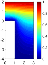
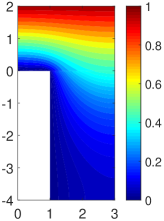
Figure 9: Planar ($xz$) projection of the solution $u(r,z)$ for $L_{1}=4$, $R_{1}=1$, $L_{2}=2$, $R_{2}=3$, and two values of the base reactivity: $\kappa=\infty$ (left) and $\kappa=0$ (right). We used the truncation order $N=10$.

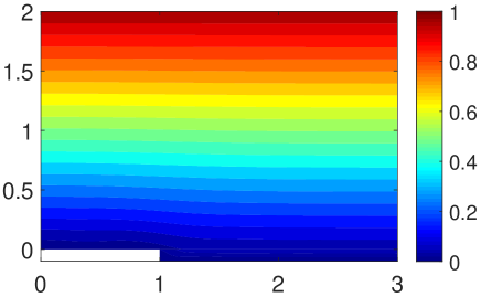
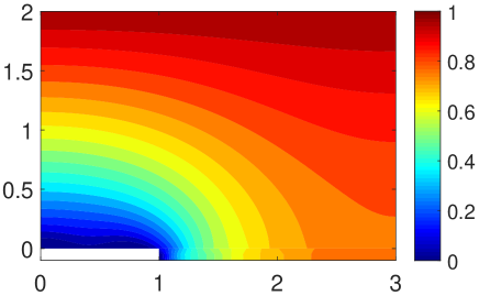
Figure 10: Planar ($xz$) projection of the solution $u(r,z)$ for $L_{1}=0.1$, $R_{1}=1$, $L_{2}=2$, $R_{2}=3$, and two values of the base reactivity: $\kappa=\infty$ (top) and $\kappa=0$ (bottom). We used the truncation order $N=10$.

It is also instructive to consider the concentration averaged over the cross-section (denoted by bar):

$$\overline{u}_{2}(z)=\frac{2\pi}{\pi R_{2}^{2}}\int\limits_{0}^{R_{2}}dr\,r\,u_{2}(r,z)=1-c_{0,2}\,\frac{L_{2}-z}{L_{2}}$$ (56)

and

$$\overline{u}_{1}(z) =\frac{2\pi}{\pi(R_{2}^{2}-R_{1}^{2})}\int\limits_{R_{1}}^{R_{2}}dr\,r\,u_{1}(r,z)$$

$$=\frac{2}{1-\rho^{2}}\sum\limits_{n=0}^{\infty}c_{n,1}\frac{s_{n,1}(z)}{s_{n,1}(0)}\int\limits_{\rho}^{1}d\bar{r}\,\bar{r}\,v_{n,1}(\bar{r})$$

$$=\frac{2}{1-\rho^{2}}\sum\limits_{n=0}^{\infty}c_{n,1}\frac{s_{n,1}(z)}{s_{n,1}(0)}\frac{\rho v^{\prime}_{n,1}(\rho)}{\alpha_{n,1}^{2}}\,,$$ (57)

where we used

$$\int\limits_{\rho}^{1}d\bar{r}\,\bar{r}\,v_{n,1}(\bar{r})=\frac{\rho\,v^{\prime}_{n,1}(\rho)}{\alpha_{n,1}^{2}}$$ (58)

due to the boundary conditions. While the averaged solution in the upper part is indeed linear, this is not true for the lower part.

A.2 Total flux

The total flux can be found as

$$J =2\pi c_{0}\int\limits_{0}^{R_{2}}dr\,r\,(D\partial_{z}u_{2})_{z=L_{2}}$$

$$=2\pi Dc_{0}\int\limits_{0}^{R_{2}}dr\,r\,\sum\limits_{n=0}^{\infty}c_{n,2}v_{n,2}(r/R_{2})\frac{B_{n}^{(2)}}{R_{2}}$$

$$=\frac{\pi Dc_{0}R_{2}^{2}}{L_{2}}\,c_{0,2}\,,$$ (59)

where $c_{0}$ is the imposed concentration of particles at the top, and we used the orthogonality of functions $\{v_{n,2}(\bar{r})\}$. One sees that the coefficient $c_{0,2}$ incorporates the sophisticated dependence of $J$ on the geometric parameters $L_{1}$, $R_{1}$, $L_{2}$, and $R_{2}$.

The structure of the exact solution reveals how different geometric parameters can affect the concentration and the total flux. In particular, the pillar height $L_{1}$ enters only via $B_{n}^{(1)}$, the distance to the source $L_{2}$ enters only via $B_{n}^{(2)}$, so that the matrix $A$ does not depend on $L_{1}$ and $L_{2}$. In the limit $L_{2}\to\infty$, one gets $B_{n}^{(2)}\to\alpha_{n,2}$ for all $n>0$. In fact, Eq. (47a) implies that if $L_{2}\gg R_{2}$, $\mathrm{ctanh}(\alpha_{n,2}L_{2}/R_{2})$ for $n>0$ can be replaced by $1$, and the error of this replacement is exponentially small (note that $\alpha_{n,2}\geq\alpha_{1,2}\approx 3.8317$ for $n\geq 1$). In other words, the elements $B_{n}^{(2)}$ does not depend on $L_{2}$ whenever $L_{2}\gg R_{2}$, except for $B_{0}^{(2)}=R_{2}/L_{2}$.

This property suggests to treat separately the equations for $n=0$ and $n>0$ in the system (54). Let us denote by $W^{\prime}$ the reduced matrix obtained by removing from $W$ the column and the row corresponding to $n=0$. More explicitly, we rewrite Eq. (54) as

$$c_{0,2}+W_{0,0}c_{0,2}+\sum\limits_{n=1}^{\infty}W_{0,n}c_{n,2} =1,$$

$$c_{k,2}+\sum\limits_{n=1}^{\infty}W_{k,n}c_{n,2} =-W_{k,0}c_{0,2}\quad(k=1,\ldots),$$

solve the second set of equations by inverting the matrix $I+W^{\prime}$, substitute the solution in the first line and then express $c_{0,2}$ as

$$c_{0,2}=\biggl{(}1+W_{0,0}-\sum\limits_{k,k^{\prime}=1}^{\infty}W_{0,k}\bigl{[}(I+W^{\prime})^{-1}\bigr{]}_{k,k^{\prime}}W_{k^{\prime},0}\biggr{)}^{-1}.$$ (60)

Importantly, both terms $W_{0,0}$ and $W_{k^{\prime},0}$ are proportional to $R_{2}/L_{2}$ due to Eq. (47b). We can therefore represent this coefficient as

$$c_{0,2}=\frac{1}{1+z_{0}/L_{2}}\,,$$ (61)

where

$$z_{0}=L_{2}\biggl{(}W_{0,0}-\sum\limits_{k,k^{\prime}=1}^{\infty}W_{0,k}\bigl{[}(I+W^{\prime})^{-1}\bigr{]}_{k,k^{\prime}}W_{k^{\prime},0}\biggr{)}.$$ (62)

While the representation (61) is valid for any $L_{2}$, its main advantage is that $z_{0}$ rapidly approaches a constant as $L_{2}\to\infty$, allowing one to eliminate this geometric parameter.

A.3 Trapping efficiency of the pillar

In order to quantify the trapping efficiency of the pillar, it is instructive to calculate the flux of particles absorbed on the top of the pillar:

$$J_{\rm top} =2\pi c_{0}\int\limits_{0}^{R_{1}}dr\,r\,(D\partial_{z}u)_{z=0}$$

$$=2\pi Dc_{0}\int\limits_{0}^{R_{1}}dr\,r\sum\limits_{n=0}^{\infty}c_{n,2}v_{n,2}(r/R_{2})\frac{B_{n}^{(2)}}{R_{2}}$$

$$=2\pi Dc_{0}R_{1}\sum\limits_{n=0}^{\infty}c_{n,2}B_{n}^{(2)}\frac{J_{1}(\alpha_{n,2}\rho)}{\alpha_{n,2}J_{0}(\alpha_{n,2})}\,.$$ (63)

To eliminate the dependence on the distance $L_{2}$, one can express the coefficients $c_{n,2}$ in terms of $c_{0,2}$:

$$J_{\rm top} =\pi Dc_{0}R_{1}c_{0,2}\frac{R_{2}}{L_{2}}\biggl{(}\rho-2\sum\limits_{n=1}^{\infty}B_{n}^{(2)}\frac{J_{1}(\alpha_{n,2}\rho)}{\alpha_{n,2}J_{0}(\alpha_{n,2})}$$

$$\times\biggl{(}\sum\limits_{k=1}^{\infty}\bigl{[}(I+W^{\prime})^{-1}\bigr{]}_{n,k}\frac{W_{k,0}L_{2}}{R_{2}}\biggr{)}\,,$$ (64)

where we wrote explicitly the term with $n=0$ due to $\alpha_{0,2}=0$. Rescaling this expression by the total flux $J$ eliminates $c_{0,2}$, yielding

$$\frac{J_{\rm top}}{J} =\rho\biggl{(}\rho-2\sum\limits_{n,k=1}^{\infty}B_{n}^{(2)}\frac{J_{1}(\alpha_{n,2}\rho)}{\alpha_{n,2}J_{0}(\alpha_{n,2})}$$

$$\times\bigl{[}(I+W^{\prime})^{-1}\bigr{]}_{n,k}\frac{W_{k,0}L_{2}}{R_{2}}\biggr{)}.$$ (65)

As $W_{k,0}$ is proportional to $R_{2}/L_{2}$, the factor $L_{2}/R_{2}$ is compensated, and we conclude that the ratio $J_{\rm top}/J$ does not almost depend on $L_{2}$ whenever $L_{2}\gg R_{2}$. In other words, the distance to a remote source does not affect the fraction of particles absorbed on the top of the pillar that allows us to define

$$\eta_{\kappa}(\rho,h)=\lim\limits_{L_{2}\to\infty}\frac{J_{\rm top}}{J}\,.$$ (66)

When $L_{2}/R_{2}\gg 1$, one has $B_{n}^{(2)}\approx\alpha_{n,2}$ and the factor $B_{n}^{(2)}\frac{J_{1}(\alpha_{n,2}\rho)}{\alpha_{n,2}J_{0}(\alpha_{n,2})}$ exhibits oscillations. Even though the series (65) remains well-defined, its convergence can be rather slow, especially for small $\rho$ and large $h$. As a consequence, getting the asymptotic behavior of $\eta_{0}(\rho,\infty)/\rho$ in the limit $\rho\to 0$ can be difficult, even numerically (see Fig. 6(b) and the related discussion).

Similarly, we can compute the flux on the base:

$$J_{\rm base} =2\pi c_{0}\int\limits_{R_{1}}^{R_{2}}dr\,r(D\partial_{z}u)_{z=-L_{1}}$$

$$=2\pi Dc_{0}R_{2}^{2}\sum\limits_{n=0}^{\infty}c_{n,1}\frac{\alpha_{n,1}}{R_{2}s_{n,1}(0)}\int\limits_{\rho}^{1}d\bar{r}\,\bar{r}\,v_{n,1}(\bar{r})$$

$$=2\pi Dc_{0}R_{1}\sum\limits_{n=0}^{\infty}c_{n,1}\frac{v^{\prime}_{n,1}(\rho)}{\alpha_{n,1}s_{n,1}(0)}.$$

Expressing $c_{n,1}$ in terms of $c_{n,2}$ and exchanging the order of summations, one gets

$$J_{\rm base} =\pi Dc_{0}R_{2}\sum\limits_{n=0}^{\infty}c_{n,2}V_{n}B_{n}^{(2)},$$

where

$$V_{n}=2\rho\sum\limits_{n^{\prime}=0}^{\infty}\frac{v^{\prime}_{n^{\prime},1}(\rho)}{\alpha_{n^{\prime},1}s_{n^{\prime},1}(0)}B_{n^{\prime}}^{(1)}A_{n^{\prime},n}.$$ (67)

As previously, we separate the term with $n=0$ from the remaining contributions, express $c_{n,2}$ in terms of $c_{0,2}$, and divide by the total flux to get the fraction of particles absorbed on the base:

$$\frac{J_{\rm base}}{J}=V_{0}-\sum\limits_{k,n=1}^{\infty}V_{n}B_{n}^{(2)}\bigl{[}(I+W^{\prime})^{-1}\bigr{]}_{n,k}\frac{W_{k,0}L_{2}}{R_{2}}\,.$$ (68)

Since this expression does not almost depend on $L_{2}$ whenever $L_{2}\gg R_{2}$, we define the fraction of particles absorbed by the base in the limit $L_{2}\to\infty$:

$$\eta^{\prime}_{\kappa}(\rho,h)=\lim\limits_{L_{2}\to\infty}\frac{J_{\rm base}}{J}\,.$$ (69)

A.4 Thin pillar asymptotic behavior

In this section, we derive the asymptotic behavior of the total flux in the limit $R_{1}\to 0$. The radius $R_{1}$ affects the solution of the problem in the domain $\Omega_{1}$, in particular, the solutions $\{\alpha_{n,1}\}$ of Eq. (40) and thus the matrix elements of $A$ and $B^{(1)}$.

First of all, we stress that the solutions $\{\alpha_{n,1}\}$ determine the eigenvalues of the two-dimensional Laplace operator in the cross section of the tube, i.e., in the annulus between the inner absorbing circle of radius $R_{1}$ and the outer reflecting circle of radius $R_{2}$. In the limit $R_{1}\to 0$, the absorbing circle can be treated as a “strong” perturbation of the disk of radius $R_{2}$ Mazya85 ; Ward93 . As a consequence, the eigenvalues of the “perturbed” problem approach those of the “unperturbed” problem, which are determined by $\alpha_{n,2}$, i.e., $\alpha_{n,1}\to\alpha_{n,2}$ for all $n$. As $\alpha_{n,2}$ are strictly positive for all $n>0$, one can simply substitute $\alpha_{n,1}$ by $\alpha_{n,2}$ in the leading-order approximation. In contrast, the approach of $\alpha_{0,1}$ to $\alpha_{0,2}=0$ determines the asymptotic behavior of the total flux.

Using the asymptotic behavior of the Bessel functions (see p. 974 in Gradsteyn ), we expand Eq. (40) as

$$0=\frac{Y_{1}(\alpha_{0,1})}{J_{1}(\alpha_{0,1})}-\frac{2}{\pi}\biggl{(}\ln(\alpha_{0,1}\rho/2)+\gamma+\ldots\biggr{)},$$

where $\gamma\approx 0.5772$ is the Euler constant, and we neglected higher-order terms in $\rho$. In order to compensate the divergent term $\ln\rho$, $\alpha_{0,1}$ should vanish. Expanding the ratio

$$\frac{Y_{1}(\alpha_{0,1})}{J_{1}(\alpha_{0,1})}\approx-\frac{4}{\pi}\biggl{(}\frac{1}{\alpha_{0,1}^{2}}-\frac{1}{2}(\ln(\alpha_{0,1}/2)+\gamma)+\frac{3}{8}\biggr{)}+\ldots$$ (70)

we get in the leading order in $\rho$

$$\alpha_{0,1}\approx\frac{\sqrt{2}}{\sqrt{\ln(1/\rho)-3/4}}\quad(\rho\to 0).$$ (71)

One sees that $\alpha_{0,1}$ indeed vanishes with $\rho$ but extremely slowly. This relation is also consistent with the general asymptotic behavior of the Laplacian eigenvalues in planar domains Mazya85 ; Ward93 .

Similarly, the associated eigenfunctions $v_{k,1}(\bar{r})$ approach $\sqrt{2}\,v_{k,2}(\bar{r})$ as $R_{1}\to 0$, but this approach can be logarithmically slow too Ward93 . As a consequence, the matrix $A$, whose elements were defined in Eq. (48) as a weighted scalar product of these functions, approaches $I/\sqrt{2}$, where $I$ is the identity matrix. In the leading order, one gets thus

$$W_{k,k^{\prime}}\approx\delta_{k,k^{\prime}}B_{k}^{(1)}B_{k^{\prime}}^{(2)}\,,$$ (72)

and the diagonal structure of this matrix allows for the explicit inversion of $I+W$. We get therefore

$$c_{0,2}\approx\frac{1}{1+\frac{R_{2}}{L_{2}}B_{0}^{(1)}}\qquad(\rho\to 0),$$ (73)

from which Eq. (61) implies

$$\zeta_{\kappa}(\rho,h)\approx B_{0}^{(1)}\qquad(\rho\to 0).$$ (74)

Using the definition (50) of $B_{n}^{(1)}$, we deduce the asymptotic approximation (23). Together with Eq. (71) for $\alpha_{0,1}$, we got the fully explicit approximation for the dimensionless offset $\zeta_{\kappa}(\rho,h)$ in the limit $\rho\to 0$.

A.5 The limit of an absorbing disk

As $L_{1}\to 0$, the pillar shrinks to an absorbing disk on the partially reactive base. Let us assume that $\kappa>0$. In this limit, one has $B_{n}^{(1)}=1/\kappa$ so that

$$W_{j,n} =\frac{2B_{n}^{(2)}}{\kappa}\int\limits_{\rho}^{1}d\bar{r}_{1}\bar{r}_{1}v_{j,2}(\bar{r}_{1})\int\limits_{\rho}^{1}d\bar{r}_{2}v_{n,2}(\bar{r}_{2})$$

$$\times\underbrace{\sum\limits_{n^{\prime}=0}^{\infty}\bar{r}_{2}v_{n^{\prime},1}(\bar{r}_{1})v_{n^{\prime},1}(\bar{r}_{2})}_{=\delta(\bar{r}_{1}-\bar{r}_{2})}$$

$$=\frac{2B_{n}^{(2)}}{\kappa}\int\limits_{\rho}^{1}d\bar{r}\,\bar{r}\,v_{j,2}(\bar{r})\,v_{n,2}(\bar{r}),$$

where we used the completeness relation for eigenfunctions $\{v_{n,1}(\bar{r})\}$. The last integral can be computed exactly, in analogy to Eq. (51):

$$W_{j,n}=\frac{2B_{n}^{(2)}}{\kappa}\rho\frac{v_{j,2}(\rho)v^{\prime}_{n,2}(\rho)-v_{n,2}(\rho)v^{\prime}_{j,2}(\rho)}{\alpha_{n,2}^{2}-\alpha_{j,2}^{2}}$$ (75)

for $j\neq n$. In turn, for $j=n$, one can use the following identity

$$\int\limits dr\,r\,J_{\nu}^{2}(\alpha r) =\frac{r^{2}}{2}\biggl{(}J_{\nu}^{2}(\alpha r)-J_{\nu-1}(\alpha r)J_{\nu+1}(\alpha r)\biggr{)}$$

$$=\frac{r^{2}}{2}\biggl{(}J_{\nu}^{2}(\alpha r)-\biggl{(}\frac{\nu J_{\nu}(\alpha r)}{\alpha r}\biggr{)}^{2}+[J^{\prime}_{\nu}(\alpha r)]^{2}\biggr{)}.$$

Setting $\nu=0$, we find

$$\int\limits_{\rho}^{1}d\bar{r}\,\bar{r}\,v_{n,2}^{2}(\bar{r}) =\frac{r^{2}}{2}\biggl{(}v_{n,2}^{2}(\bar{r})+\frac{[v^{\prime}_{n,2}(\bar{r})]^{2}}{\alpha_{n,2}^{2}}\biggr{)}_{\bar{r}=\rho}^{1}$$

$$=\frac{1}{2}-\frac{\rho^{2}}{2}\biggl{(}v_{n,2}^{2}(\rho)+\frac{[v^{\prime}_{n,2}(\rho)]^{2}}{\alpha_{n,2}^{2}}\biggr{)},$$

where we used boundary conditions. We get then

$$W_{n,n}=\frac{B_{n}^{(2)}}{\kappa}\biggl{(}1-\rho^{2}\biggl{(}v_{n,2}^{2}(\rho)+\frac{[v^{\prime}_{n,2}(\rho)]^{2}}{\alpha_{n,2}^{2}}\biggr{)}\biggr{)}.$$ (76)

We stress that the elements of the matrix $W$ are fully explicit in this case. The inversion of the matrix $I+W$ determines the coefficients $\{c_{k,2}\}$ and thus the whole solution for an absorbing disk on a partially reactive base.

In the trivial limit $\kappa=\infty$, one gets $W=0$, from which $c_{k,2}=\delta_{k,0}$ and one retrieves the expected solution $u(r,z)=z/L_{2}$ that corresponds to the whole absorbing surface at the bottom. In turn, the opposite limit $\kappa\to 0$ is mathematically more difficult as the contribution of the matrix $W$ becomes dominant but the identity matrix $I$ cannot be neglected in $(I+W)^{-1}$ (as $W$ is expected to be non-invertible).

For the reflecting base ($\kappa=0$), Fig. 3 illustrated that the offset can be very accurately approximated by the Fock’s function, see Eq. (17). We expect that this result can be deduced from our exact solution. On the one hand, one can attempt to undertake the limit $\kappa\to 0$ of the matrix $(I+W^{\prime})^{-1}$ by using the exact explicit form (75, 76) of the matrix elements $W_{k,n}$. On the other hand, one can first set $\kappa=0$ in Eq. (50) to get $B_{n}^{(1)}=\mathrm{ctanh}(\alpha_{n,1}h)/\alpha_{n,1}$ and then analyze the asymptotic behavior $h\to 0$. The major technical difficulty is that one cannot replace this expression by its leading-order $B_{n}^{(1)}\approx 1/(h\alpha_{n,1}^{2})$. In fact, for any fixed $h$, this approximation is valid for $n\lesssim n_{\rm max}$ with some $n_{\rm max}$ but one still has $B_{n}^{(1)}\approx 1/\alpha_{n,1}$ for $n\gg n_{\rm max}$. As a consequence, the limit $h\to 0$ resembles the semi-classical asymptotic analysis of a hamiltonian $h^{2}\Delta+V$ with a bounded potential $V$ in quantum mechanics, and thus requires finer asymptotic tools. Moreover, one generally needs very large truncation orders to get accurate numerical results.

The same difficulty emerges in the limit $R_{2}\to\infty$, which is equivalent to the double limit $\rho\to 0$ and $h\to 0$ with $h/\rho$ being fixed.

A.6 Extensions

While we focused on solving the particular boundary value problem (5), the proposed method can be easily extended in several directions.

i) The Laplace equation $\Delta u=0$ can be replaced by the modified Helmholtz equation, $(\Delta-p/D)u=0$. In this case, it is sufficient to replace $\alpha_{n,1}$ by $\alpha^{\prime}_{n,1}=(\alpha_{n,1}^{2}+p/D)^{1/2}$ in Eqs. (35, 50) and $\alpha_{n,2}$ by $\alpha^{\prime}_{n,2}=(\alpha_{n,2}^{2}+p/D)^{1/2}$ in Eqs. (43, 47a). These replacements ensure that the series representations (34, 41) satisfy the modified Helmholtz equation. The rest of computations remains unchanged (see details in Grebenkov_2023 ). Moreover, an inverse Laplace transform of $u$ with respect to $p$ gives the time evolution of the concentration governed by the diffusion equation,

$$\partial_{t}u=D\Delta u\quad\textrm{in}~{}\Omega,$$ (77)

with the initial condition $u(r,z,t=0)=0$, and the same boundary conditions as in Eqs. (5). This equation also describes heat propagation from the “hot” top plane at $z=L_{2}$ (kept at a constant temperature $1$) to the bottom spiky support (kept at a constant temperature $0$).

ii) The homogeneous boundary condition $u(r,L_{2})=1$ on the top disk can be replaced by $u(r,L_{2})=f(r)$ with a given function $f(r)$. For this purpose, it is sufficient to replace the right-hand side of Eq. (54) by

$$\int\limits_{0}^{1}d\bar{r}\,\bar{r}\,v_{n,2}(\bar{r})\,f(\bar{r}R_{2}).$$ (78)

One easily obtains therefore a general form of the source term.

Moreover, setting $f(r)=0$ yields a homogeneous system of linear equations, which has either none or infinitely many nontrivial solutions, according to whether $\det(I+W)\neq 0$ or not. For the Laplace equation, the only solution is $c_{k,2}=0$ for all $k$, i.e., $u(r,z)\equiv 0$. In turn, for the modified Helmholtz equation, the condition $\det(I+W)=0$ allows one to determine the eigenvalues of the Laplace operator in this domain; the associated eigenfunctions are given $u(r,z)$.

iii) The Dirichlet boundary condition $u(r,L_{2})=1$ can be replaced by Neumann boundary condition $(\partial_{z}u(r,z))_{z=L_{2}}=0$. For this purpose, the functions $s_{n,2}(z)$ from Eq. (43) should be replaced by

$$s_{n,2}^{\rm N}(z)=\frac{\cosh(\alpha_{n,2}(L_{2}-z)/R_{2})}{\cosh(\alpha_{n,2}L_{2}/R_{2})}\,.$$ (79)

Accordingly, one would have

$$B_{n}^{(2),\rm N}=-R_{2}\bigl{(}\partial_{z}s_{n,2}^{{\rm N}}(z)\bigr{)}_{z=0}=\alpha_{n,2}\tanh(\alpha_{n,2}L_{2}/R_{2}).$$ (80)

In addition, one removes $1$ from Eq. (41) and sets the right-hand side of Eq. (54) to $0$. One can similarly treat the Robin boundary condition at $z=L_{2}$. Together with the above modification for the modified Helmholtz equation, the solution $u(r,z)$ of the modified problem can be interpreted as the Laplace transform of the probability density function (PDF) of the first-passage time to the absorbing pillar.

(iv) The mode matching method is also applicable to more complicated geometric settings. In particular, one can consider a cylindrical pillar of arbitrary cross section $\Gamma_{1}$ inside a collinear outer tube of arbitrary cross section $\Gamma_{2}$ (such that $\Gamma_{1}\subset\Gamma_{2}$). In this case, the radial functions $v_{n,1}(r)$ are replaced by the normalized eigenfunctions of the two-dimensional Laplace operator in the annular domain $\Gamma_{2}\backslash\Gamma_{1}$, with Dirichlet boundary condition on $\partial\Gamma_{1}$ and Neumann boundary condition on $\partial\Gamma_{2}$. The associated eigenvalues $\lambda_{n,1}$ give $\alpha_{n,1}/R_{2}=\sqrt{\lambda_{n,1}}$. Similarly, $v_{n,2}(r)$ are replaced by the normalized eigenfunctions of the two-dimensional Laplace operator in $\Gamma_{2}$, with Neumann boundary condition on $\partial\Gamma_{2}$, and $\alpha_{n,2}/R_{2}=\sqrt{\lambda_{n,2}}$. The rest of computations remains unchanged; in particular, the total flux is still given by Eq. (1), in which $\pi R_{2}^{2}$ is replaced by the area $|\Gamma_{2}|$ of the tube cross section, and the offset parameter $z_{0}$ is still given by Eq. (62). Even though this extension is elementary, the solution looses its analytic character because the eigenfunctions and eigenvalues of the Laplace operator are generally not known explicitly Grebenkov13 , except for a few cases such as a disk or an annulus between two concentric circles (as we considered in this paper). Nevertheless, the universal structure of this extended solution allows one to draw some general conclusions, such as the form (1) of the total flux. Moreover, the average of the solution over the cross section is still linear, as in Eq. (56). This is a consequence of the fact that the ground eigenfunction $v_{0,2}$ is constant, while the corresponding eigenvalue is $\lambda_{0,2}=0$, whatever the cross section of the tube.

The last observation provides a simple way to compute the total flux by Monte Carlo simulations. According to Eq. (56), one has $\overline{u}_{2}(0)=1-c_{0,2}$ so that the total flux is

$$J=\frac{|\Gamma_{2}|Dc_{0}}{L_{2}}\bigl{(}1-\overline{u}_{2}(0)\bigr{)}.$$ (81)

Let us recall that the solution $u(\mathbf{x})$ can be interpreted as the splitting probability: if a particle starts from $\mathbf{x}$, this is the probability of hitting the top cross-section at $z=L_{2}$ before being absorbed on the pillar (or on the base). If the starting point is uniformly distributed on the tube cross section at $z=0$, the average $\overline{u}_{2}(0)$ is again the splitting probability, which can be easily accessed via Monte Carlo simulations. For this purpose, one can generate $M$ random trajectories of a diffusing particle started uniformly at $z=0$, and count how many of them, $M_{\rm top}$, reached the level $z=L_{2}$ before being absorbed. When $M$ is large, $M_{\rm top}/M$ approximates $\overline{u}_{2}(0)$, and thus determines the total flux.

References

- (1) S. Rice, Diffusion-Limited Reactions (Elsevier, Amsterdam, 1985).
- (2) B. D. Hughes, Random Walks and Random Environments, (Clarendon Press, Oxford, 1995).
- (3) S. Redner, A Guide to First-Passage Processes (Cambridge University Press, 2001).
- (4) P. L. Krapivsky, S. Redner, and E. Ben-Naim, A Kinetic View of Statistical Physics (Cambridge University Press, 2010).
- (5) Z. Schuss, Brownian Dynamics at Boundaries and Interfaces in Physics, Chemistry and Biology (Springer, New York, 2013).
- (6) R. Metzler, G. Oshanin, and S. Redner (Eds), First-Passage Phenomena and Their Applications (World Scientific Press, Singapore, 2014).
- (7) K. Lindenberg, R. Metzler, and G. Oshanin (Eds), Chemical Kinetics: Beyond the Textbook (World Scientific, New Jersey, 2019).
- (8) D. S. Grebenkov, NMR Survey of Reflected Brownian Motion, Rev. Mod. Phys. 79, 1077-1137 (2007).
- (9) O. Bénichou and R. Voituriez, From first-passage times of random walks in confinement to geometry-controlled kinetics, Phys. Rep. 539, 225-284 (2014).
- (10) D. S. Grebenkov, Paradigm Shift in Diffusion-Mediated Surface Phenomena, Phys Rev Lett. 125, 078102 (2020).
- (11) D. ben-Avraham and S. Havlin, Diffusion and Reactions in Fractals and Disordered Systems (Cambridge University Press, 2010)
- (12) M.-O. Coppens, The effect of fractal surface roughness on diffusion and reaction in porous catalysts: from fundamentals to practical applications, Cat. Today 53, 225 (1999).
- (13) M. Filoche, B. Sapoval, J. S. Andrade Jr., Deactivation Dynamics of Rough Catalytic Surfaces, AIChE 51, 998 (2005).
- (14) M. Filoche, D. S. Grebenkov, J. S. Andrade Jr., and B. Sapoval, Passivation of irregular surfaces accessed by diffusion, Proc. Nat. Acad. Sci. 105, 7636 (2008).
- (15) T. A. Witten Jr. and L. M. Sander, Diffusion-Limited Aggregation, a Kinetic Critical Phenomenon, Phys. Rev. Lett. 47, 1400 (1981).
- (16) T. C. Halsey and M. Leibig, Electrodeposition and diffusion-limited aggregation, J. Chem. Phys. 92, 3756 (1990).
- (17) M. Filoche and B. Sapoval, Diffusion-Reorganized Aggregates: Attractors in Diffusion Processes, Phys. Rev. Lett. 85, 5118 (2000).
- (18) M.-O. Bernard, J. Garnier, and J.-F. Gouyet, Laplacian growth of parallel needles: A Fokker-Planck equation approach, Phys. Rev. E 64, 041401 (2001).
- (19) R. E. Goldstein, T. C. Halsey, and M. Leibig, Thermodynamics of Rough Colloidal Surfaces, Phys. Rev. Lett. 66, 1551 (1991).
- (20) B. Duplantier, Can One ’Hear’ the Thermodynamics of a (Rough) Colloid, Phys. Rev. Lett. 66, 1555 (1991).
- (21) R. J. Garde and K. G. Ranga Raju, Mechanics of Sediment Transportation and Alluvial Stream Problems (Wiley Eastern: New Delhi, India, 1977).
- (22) G. Boffetta, A. Celani, D. Dezzani, and A. Seminara, How winding is the coast of Britain? Conformal invariance of rocky shorelines, Geop. Res. Lett. 35, L03615 (2008).
- (23) M. G. Blyth and C. Pozrikidis, Diffusive transport across irregular and fractal walls, Proc. R. Soc. Lond. A 442, 571-58 (1993).
- (24) M. G. Blyth and C. Pozrikidis, Heat conduction across irregular and fractal-like surfaces, Int. J. Heat Mass Trans. 46, 1329-1339 (2003).
- (25) J. S. Andrade Jr., E. A. A. Henrique, M. P. Almeida, and M. H. A. S. Costa, Heat transport through rough channels, Physica A 339, 296 (2004).
- (26) A. Rozanova-Pierrat, D. S. Grebenkov, and B. Sapoval, Faster Diffusion across an Irregular Boundary, Phys. Rev. Lett. 108, 240602 (2012).
- (27) S. H. Liu, Fractal Model for the ac Response of a Rough Interface, Phys. Rev. Lett. 55, 529 (1985).
- (28) B. Sapoval, J.-N. Chazalviel, and J. Peyrière, Electrical response of fractal and porous interfaces, Phys. Rev. A 38, 5867 (1988).
- (29) R. Blender, W. Dieterich, T. Kirchhoff, and B. Sapoval, Impedance of Fractal Interfaces, J. Phys. A 23, 1225 (1990).
- (30) E. Chassaing, B. Sapoval, G. Daccord, and R. Lenormand, Experimental study of the impedance of blocking quais-fractal and rough electrodes, J. Electroanal. Chem. 279, 67 (1990).
- (31) T. C. Halsey and M. Leibig, The double layer impedance at a rough surface. Theoretical results, Ann. Phys. 219, 109 (1992).
- (32) D. S. Grebenkov, M. Filoche, and B. Sapoval, Mathematical Basis for a General Theory of Laplacian Transport towards Irregular Interfaces, Phys. Rev. E 73, 021103 (2006).
- (33) B. Sapoval, General Formulation of Laplacian Transfer Across Irregular Surfaces, Phys. Rev. Lett. 73, 3314 (1994).
- (34) P. Levitz, D. S. Grebenkov, M. Zinsmeister, K. M. Kolwankar, and B. Sapoval, Brownian flights over a fractal nest and first passage statistics on irregular surfaces, Phys. Rev. Lett. 96, 180601 (2006).
- (35) D. A. Lauffenburger and J. J. Linderman, Receptors: Models for Binding, Trafficking, and Signaling (Oxford University Press, New York, 1993).
- (36) P. C. Bressloff and J. M. Newby, Stochastic models of intracellular transport, Rev. Mod. Phys. 85, 135-196 (2013).
- (37) F. Höfling and T. Franosch, Anomalous transport in the crowded world of biological cells, Rep. Progr. Phys. 76, 046602 (2013).
- (38) D. S. Grebenkov, M. Filoche, B. Sapoval, and M. Felici, Diffusion-Reaction in Branched Structures: Theory and Application to the Lung Acinus, Phys. Rev. Lett. 94, 050602 (2005).
- (39) A. Serov, C. Salafia, D. S. Grebenkov, and M. Filoche, The Role of Morphology in Mathematical Models of Placental Gas Exchange, J. Appl. Physiol. 120, 17-28 (2016).
- (40) B. Sapoval, M.-Y. Kang, and A. T. Dinh-Xuan, Modeling of Gas Exchange in the Lungs, Compr. Physiol. 11, 1289-1314 (2021).
- (41) H. C. Berg and E. M. Purcell, Physics of chemoreception, Biophys. J. 20, 193 (1977).
- (42) R. Zwanzig, Diffusion-controlled ligand binding to spheres partially covered by receptors: an effective medium treatment, Proc. Natl. Acad. Sci. USA. 87, 5856-5857 (1990).
- (43) R. Zwanzig and A. Szabo, Time dependent rate of diffusion-influenced ligand binding to receptors on cell surfaces, Biophys. J. 60, 671 (1991).
- (44) B. I. Kharisov, O. V. Kharissova, B. O. García, Y. P. Méndez, and I. G. de la Fuente, State of the art of nanoforest structures and their applications, Proc. Roy. Soc. Adv. 5, 105507 (2015).
- (45) A. M. J. Davis and E. Lauga, Hydrodynamic friction of fakir–like superhydrophobic surfaces, J. Fluid Mech. 661, 402-411 (2010).
- (46) G. Z. Ramon, M. C. Y. Wong, E. M. V. Hoek, Transport through composite membrane, part 1: Is there an optimal support membrane? J. Membr. Sci. 415-416, 298-305 (2012).
- (47) G. Z. Ramon and E. M. V. Hoek, Transport through composite membranes, part 2: Impacts of roughness on permeability and fouling, J. Membr. Sci. 425-426, 141-148 (2013).
- (48) P. R. Nair and M. A. Alam, Dimensionally frustrated diffusion towards fractal adsorber, Phys. Rev. Lett. 99, 256101 (2007).
- (49) T. Wei, Z. Tang, Q. Yu, and H. C. Smart, Antibacterial Surfaces with Switchable Bacteria-Killing and Bacteria-Releasing Capabilities, ACS Appl. Mat. Int. 9, 43, 37511-37523 (2017).
- (50) G. Chen, R. Guan, M. Shi, X. Dai, H. Li, N. Zhou, D. Chen, and H. Mao, A nanoforest-based humidity sensor for respiration monitoring, Microsystems and Nanoeng. 8, 44 (2022).
- (51) E. Borberg, M. Zverzhinetsky, A. Krivitsky, A. Kosloff, O. Heifler, G. Degabli, H. P. Soroka, R. S. Fainaro, L. Burstein, S. Reuveni, H. Diamant, V. Krivitsky, and F. Patolsky, Light-Controlled Selective Collection-and-Release of Biomolecules by an On-Chip Nanostructured Device, NanoLett. 19, 5868-5878 (2019).
- (52) A. Skvortsov and A. Walker, Trapping of diffusive particles by rough absorbing surfaces: Boundary smoothing approach, Phys. Rev. E 90, 023202 (2014).
- (53) A. T. Skvortsov, A. M. Berezhkovskii, and L. Dagdug, Trapping of diffusing particles by short absorbing spikes periodically protruding from reflecting base, J. Chem. Phys. 149, 044106 (2018).
- (54) A. T. Skvortsov, A. M. Berezhkovskii,and L. Dagdug, Trapping of diffusing particles by spiky absorbers, J. Chem. Phys. 148, 084103 (2018).
- (55) R. Gutfraind and B. Sapoval, Active surface and adaptability of fractal membranes and electrodes, J. Phys. I France 3, 1801 (1993).
- (56) Sapoval, Filoche, K. Karamanos, R. Brizzi, Can one hear the shape of an electrode? I. Numerical study of the active zone in Laplacian transfer, Eur. Phys. J. B 9, 739 (1999).
- (57) M. Filoche and B. Sapoval, Can One Hear the Shape of an Electrode? II. Theoretical Study of the Laplacian Transfer, Eur. Phys. J. B 9, 755 (1999).
- (58) M. Filoche and B. Sapoval, Transfer Across Random versus Deterministic Fractal Interfaces, Phys. Rev. Lett. 84, 5776 (2000).
- (59) N. G. Makarov, On the distortion of boundary sets under conformal mappings, Proc. London Math. Soc. 51, 369 (1985).
- (60) P. W. Jones and T. H. Wolff, Hausdorff dimension of harmonic measures in the plane, Acta Math 161, 131-144 (1988).
- (61) J. Bourgain, On the Hausdorff dimension of harmonic measure in higher dimension, Invent. Math. 87, 477 (1987).
- (62) D. S. Grebenkov, A. Lebedev, M. Filoche, and B. Sapoval, Multifractal Properties of the Harmonic Measure on Koch Boundaries in Two and Three Dimensions, Phys. Rev. E 71, 056121 (2005).
- (63) D. Vandembroucq and S. Roux, Conformal mapping on rough boundaries I: Applications to harmonic problems, Phys. Rev. E 55, 6171-6185 (1997).
- (64) D. S. Grebenkov, Universal formula for the mean first passage time in planar domains, Phys. Rev. Lett. 117, 260201 (2016).
- (65) D. P. Hewett and I. J. Hewitt, Homogenized boundary conditions and resonance effects in Faraday cages, Proc. R. Soc. A 472, 20160062 (2016).
- (66) K. Sarkar and A. Prosperetti, Effective boundary conditions for the Laplace equation with a rough boundary, Proc. Royal Soc. A 451, 425-452 (1995).
- (67) M. Bruna, S. J. Chapman, and G. Z. Ramon, The effective flux through a thin-film composite membrane, EPL 110, 40005 (2015).
- (68) A. E. Lindsay, A. J. Bernoff, and M. J. Ward, First passage statistics for the capture of a Brownian particle by a structured spherical target with multiple surface traps, SIAM Multiscale Model. Simul. 15, 74-109 (2017).
- (69) A. J. Bernoff and A. E. Lindsay, Numerical approximation of diffusive capture rates by planar and spherical surfaces with absorbing pores, SIAM J. Appl. Math. 78, 266-290 (2018).
- (70) A. J. Bernoff, A. E. Lindsay, and D. D. Schmidt, Boundary Homogenization and Capture Time Distributions of Semipermeable Membranes with Periodic Patterns of Reactive Sites, SIAM Multiscale Model. Simul. 16, 1411-1447 (2018).
- (71) F. Paquin-Lefebvre, S. Iyaniwura, and M. J. Ward, Asymptotics of the principal eigenvalue of the Laplacian in 2D periodic domains with small traps, Eur. J. Appl. Math. 33, 646-673 (2022).
- (72) K. H. Keller and T. R. Stein, A Two-Dimensional Analysis of Porous Membrane Transport, Math. Biosci. 1, 421-437 (1967).
- (73) D. S. Grebenkov and D. Krapf, Steady-state reaction rate of diffusion-controlled reactions in sheets, J. Chem. Phys. 149, 064117 (2018).
- (74) A. Delitsyn and D. S. Grebenkov, Mode matching methods in spectral and scattering problems, Quart. J. Mech. Appl. Math. 71, 537-580 (2018).
- (75) A. Delitsyn and D. S. Grebenkov, Resonance scattering in a waveguide with identical thick perforated barriers, Appl. Math. Comput. 412, 126592 (2022).
- (76) O. Bénichou, D. S. Grebenkov, P. Levitz, C. Loverdo, R. Voituriez, Mean first-passage time of surface-mediated diffusion in spherical domains, J. Stat. Phys. 142, 657-685 (2011).
- (77) T. Calandre, O. Bénichou, D. S. Grebenkov, and R. Voituriez, Splitting probabilities and interfacial territory covered by 2D and 3D surface-mediated diffusion, Phys. Rev. E 89, 012149 (2014).
- (78) O. Bénichou, D. S. Grebenkov, L. Hillairet, L. Phun, R. Voituriez, and M. Zinsmeister, Mean exit time for surface-mediated diffusion: spectral analysis and asymptotic behavior, Anal. Math. Phys. 5, 321-362 (2015).
- (79) S. D. Traytak, The diffusive interaction in diffusion-limited reactions: the steady-state case, Chem. Phys. Lett. 197, 247-254 (1992).
- (80) M. Felici, M. Filoche, and B. Sapoval, Diffusional screening in the human pulmonary acinus, J. Appl. Physiol. 94, 2010 (2003).
- (81) N. McDonald and W. Strieder, Diffusion and reaction for a spherical source and sink, J. Chem. Phys. 118, 4598 (2003).
- (82) N. McDonald and W. Strieder, Competitive interaction between two different spherical sinks, J. Chem. Phys. 121, 7966 (2004).
- (83) S. D. Traytak, A. V. Barzykin, and M. Tachiya, Competition effects in diffusion-controlled bulk reactions between ions, J. Chem. Phys. 126, 144507 (2007).
- (84) J. S. Andrade Jr., A. D. Araújo, M. Filoche, and B. Sapoval, Screening Effects in Flow through Rough Channels, Phys. Rev. Lett. 98, 194101 (2007).
- (85) S. D. Traytak and D. S. Grebenkov, Diffusion-influenced reaction rates for active ’sphere-prolate spheroid’ pairs and Janus dimers, J. Chem. Phys. 148, 024107 (2018).
- (86) D. S. Grebenkov, What Makes a Boundary Less Accessible, Phys. Rev. Lett. 95, 200602 (2005).
- (87) P. Mörters and Y. Peres, Brownian Motion (Cambridge Series in Statistical and Probabilistic Mathematics, Cambridge University Press, New York, 2010).
- (88) A. T. Skvortsov, A. M. Berezhkovskii, and L. Dagdug, Steady-state flux of diffusing particles to a rough boundary formed by absorbing spikes periodically protruding from a reflecting base, J. Chem. Phys. 150, 194109 (2019).
- (89) P. A. Martin and A. T. Skvortsov, Steady State Diffusion in Tubular Structures: Assessment of One-Dimensional Models, Eur. J. App. Math. 1–18 (2022).
- (90) V. A. Fock, A theoretical investigation of the acoustical conductivity of a circular aperture in a wall put across a tube, C. R. Acad. Sci. U.R.S.S. (Doklady Akad. Nauk. SSSR) 31, 875-878 (1941).
- (91) A. T. Skvortsov, L. Dagdug, A. M. Berezhkovskii, I. R. MacGillivray, and S. M. Bezrukov, Evaluating diffusion resistance of a constriction in a membrane channel by the method of boundary homogenization, Phys. Rev. E 103, 012408 (2021).
- (92) D. S. Grebenkov and A. T. Skvortsov, Mean first-passage time to a small absorbing target in three-dimensional elongated domains, Phys. Rev. E 105, 054107 (2022).
- (93) F. G. Leppington and H. Levine, Some axially symmetric potential problems, Proc. Edinburgh Math. Soc. 18, 55-76 (1972).
- (94) H.-X. Zhou, A. Szabo, J. F. Douglas, and J. B. Hubbard, A Brownian dynamics algorithm for calculating the hydrodynamic friction and the electrostatic capacitance of an arbitrarily shaped object, J. Chem. Phys. 100, 3821 (1994).
- (95) D. S. Grebenkov and A. T. Skvortsov, Mean first-passage time to a small absorbing target in an elongated planar domain, New J. Phys. 22, 113024 (2020).
- (96) A. Chaigneau and D. S. Grebenkov, First-passage times to anisotropic partially reactive targets, Phys. Rev. E 105, 054146 (2022).
- (97) T. Sandua, G. Boldeiu, and V. Moagar-Poladian, Applications of electrostatic capacitance and charging, J. Appl. Phys. 114, 224904 (2013).
- (98) J. D. Jackson, Charge density on thin straight wire, revisited, Am. J. Phys. 68, 789 (2000).
- (99) I. C. Chang and I. Dee Chang, Potential of a Charged Axially Symmetric Conductor Inside a Cylindrical Tube, J. Appl. Phys. 41, 1967 (1970).
- (100) J.-R. Riba and F. Capelli, Analysis of Capacitance to Ground Formulas for Different High-Voltage Electrodes, Energies 11, 1090 (2018).
- (101) A. M. Berezhkovskii, Y. A. Makhnovskii, M. I. Monine, V. Yu. Zitserman, and S. Y. Shvartsman, Boundary homogenization for trapping by patchy surfaces, J. Chem. Phys. 121, 11390 (2004).
- (102) A. M. Berezhkovskii and A. V. Barzykin, Simple formulas for the trapping rate by nonspherical absorber and capacitance of nonspherical conductor, J. Chem. Phys. 126, 106102 (2007).
- (103) V. G. Maz’ya, S. A. Nazarov, and B. A. Plamenevskii, Asymptotic Expansions of the Eigenvalues of Boundary Value Problems for the Laplace Operator in Domains with Small Holes, Math. USSR. Izv 24, 321-345 (1985).
- (104) M. J. Ward and J. B. Keller, Strong Localized Perturbations of Eigenvalue Problems, SIAM J. Appl. Math. 53, 770-798 (1993).
- (105) D. S. Grebenkov, R. Metzler, and G. Oshanin, Effects of the target aspect ratio and intrinsic reactivity onto diffusive search in bounded domains, New J. Phys. 19, 103025 (2017).
- (106) S. B. Yuste, E. Abad, and K. Lindenberg, Exploration and Trapping of Mortal Random Walkers, Phys. Rev. Lett. 110, 220603 (2013).
- (107) B. Meerson and S. Redner, Mortality, Redundancy, and Diversity in Stochastic Search, Phys. Rev. Lett. 114, 198101 (2015).
- (108) D. S. Grebenkov and J.-F. Rupprecht, The escape problem for mortal walkers, J. Chem. Phys. 146, 084106 (2017).
- (109) D. S. Grebenkov and A. T. Skvorstov, Survival in a nanoforest of absorbing pillars (submitted; available online on http://arxiv.org/abs/2211.08960)
- (110) M. Z. Bazant, Exact solutions and physical analogies for unidirectional flows, Phys. Rev. Fluids 1, 024001 (2016).
- (111) M. M. Fyrillas and C. Pozrikidis, Conductive heat transport across rough surfaces and interfaces between two conforming media, Int. J. Heat Mass Trans. 44, 1789-1801 (2001).
- (112) J.-J. Marigo and A. Maurela, Homogenization models for thin rigid structured surfaces and films, J. Acoust. Soc. Am. 140, 260-273 (2016).
- (113) D. S. Grebenkov, A physicist’s guide to explicit summation formulas involving zeros of Bessel functions and related spectral sums, Rev. Math. Phys. 33, 2130002 (2021).
- (114) G. N. Watson, A Treatise on the Theory of Bessel Functions (Cambridge University Press, Cambridge, 1962).
- (115) I. S. Gradshteyn and I. M. Ryzhik, Table of Integrals, Series and Products (New York: Academic Press, 1980).
- (116) D. S. Grebenkov and B.-T. Nguyen, Geometrical structure of Laplacian eigenfunctions, SIAM Rev. 55, 601-667 (2013).