Explicit intensity control for Accented Text-to-speech

Abstract

Accented text-to-speech (TTS) synthesis seeks to generate speech with an accent (L2) as a variant of the standard version (L1). How to control the intensity of accent in the process of TTS is a very interesting research direction, and has attracted more and more attention. Recent work design a speaker-adversarial loss to disentangle the speaker and accent information, and then adjust the loss weight to control the accent intensity. However, such a control method lacks interpretability, and there is no direct correlation between the controlling factor and natural accent intensity. To this end, this paper propose a new intuitive and explicit accent intensity control scheme for accented TTS. Specifically, we first extract the posterior probability, called as “goodness of pronunciation (GoP)” from the L1 speech recognition model to quantify the phoneme accent intensity for accented speech, then design a FastSpeech2 based TTS model, named Ai-TTS, to take the accent intensity expression into account during speech generation. Experiments show that the our method outperforms the baseline model in terms of accent rendering and intensity control.

Index Terms—  Accented, Text-to-Speech (TTS), Intensity, Goodness of Pronunciation (GoP), Explicit Control

1 Introduction

Accented text-to-speech (TTS) synthesis aims to synthesis speech with foreign accent instead of native speech [1]. Note that accent is characterized by a distinctive manner of expression that is influenced by the mother tongue, social group of speakers, or spoken in a particular region [2]. Therefore, the wide adoption of speech applications, such as chatbot and movie dubbing, calls for the study of accented TTS synthesis [3]. Another important practical application is in the design of tools aimed at improving L2 phonological acquisition in language learners.

For accented TTS, some attempts tried to model the accent expression through model interpolation [4, 5, 6, 7, 8], variance information prediction [6, 7, 8], specific quinphone linguistic features [9, 10] and tone/stress embedding [10, 11], etc. However, the accent as perceived in human speech is subtle and at a fine level [12]. How to control the intensity of an accent is still an open challenge [13]. Wutiwiwatchai et al. [14] proposed an accent level adjustment mechanism for bilingual TTS synthesis, where the accent level is adjusted by means of interpolation between HMMs of native phones and HMMs of corresponding foreign phones. This method provides an effective fine-grained accent intensity control scheme, while it cannot be used in current deep learning TTS models, such as Tacotron [15, 11] and FastSpeech [16, 17] based architectures. In a recent deep learning based multilingual TTS study [1], the authors employed the domain adversarial training [18] to disentangle the accent identity from the speaker identity where the accent level can be controlled by varying the domain adversarial weight [1]. Such an adversarial weight method controls the utterance-level accent intensity of speech by using the model hyper-parameter. There is no direct and measurable correlation between the controlling factor and the natural accent intensity. The question is how to characterize the fine-grained phoneme-level accent intensity meaningfully, and employ the intensity to control the synthesis of L2 speech for state-of-the-art TTS models, which is the focus of this paper.

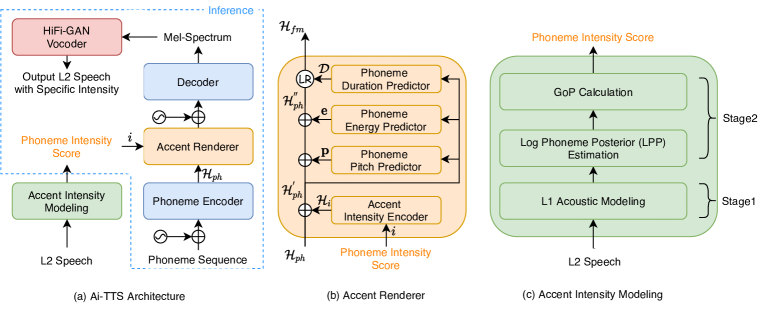
Fig. 1: The diagrams for the proposed Ai-TTS system. (a) shows the overall model architecture; (b) illustrates the detailed structure of the accent renderer, which includes the accent intensity encoder and the variance adaptor; (c) demonstrates the workflow of the accent intensity modeling.

Fortunately, we found that there is a great deal of work in the field of Computer-aided pronunciation training (CAPT) [19, 20] to measure the pronunciation of non-native learner. Most of these works assumed that acoustic properties in the learner’s pronunciation are similar to a native English speaker’s acoustics when their pronunciation similarity is high and vice-versa. Considering this, for each phoneme’s in a learner’s utterance, a representative score based on posterior probability of the phoneme models given uttered phoneme speech acoustics, called as Goodness of Pronunciation (GoP) [21, 22] was proposed and achieved remarkable performance.

Inspired by this, in this paper, we proposes a FastSpeech2 based accented TTS model, named Ai-TTS, which synthesizes L2 speech by conditioning phoneme-wise accent intensity information. To quantify the fine-grained accent intensity, we utilize a pretrained L1 speech recognition model to calculate the GoP score as the phoneme intensity score for each L2 phoneme. During inference, we can control accent expression easily by conditioning intensity labels manually. The experimental results show that our system successfully achieves better accent expressiveness and controllability than the baseline system.

The significant contributions of this work include, 1) We introduce a novel FastSpeech2 based accented TTS synthesis paradigm, named Ai-TTS, that explicitly controls the accent intensity in output speech; 2) We successfully design and implement a fine-grained accent intensity quantization method with accent speech recognition model; 3) We show that the proposed Ai-TTS framework outperforms the baseline models and generates high-quality L2-accented speech.

2 Ai-TTS: Methodology

2.1 Model Architecture

We propose a neural architecture, termed as Ai-TTS, as shown in Fig.1 (a) that consists of an accent intensity modeling module, a phoneme encoder, an accent renderer, and a decoder. The phoneme encoder and decoder are implemented on the basis of FastSpeech2 [17]. The novel accent intensity modeling module aims to learn the phoneme-level accent intensity score for the input L2 speech. Note that the accent intensity modeling module can be treated as the preprocessing operation to label the phoneme intensity score for L2 speech dataset. The phoneme encoder encodes the input phoneme sequence into phoneme embedding. The accent renderer seeks to modulate the input phoneme embeddings with the learned phoneme intensity score and various variance information (including pitch, energy and duration) towards the target accent. Note that the input phoneme intensity score enables all variance information to be affected by the fine-grained accent intensity. The decoder converts the modulated phoneme embeddings into a mel-spectrum sequence. Finally, the universal HiFi-GAN vocoder [23] is used to synthesize high-quality L2 speech.

2.2 Accent Renderer

Unlike the traditional variance adaptor in [17] just adds different variance information such as duration, pitch and energy into the phoneme embeddings, that lacks an accent controlling mechanism, our accent renderer augments the phoneme embeddings with the phoneme accent intensity scalar. The accent renderer provides phoneme-level accent information according to fine-grained accent intensity. As shown in Fig.1 (b), the accent renderer consists of 1) an accent intensity encoder, 2) a phoneme pitch predictor, 3) a phoneme energy predictor, and 4) a phoneme duration predictor.

Assume that phoneme embedding $\mathcal{H}_{ph}$ is the phoneme encoder output and the learned phoneme intensity score is $i$. We implement the accent intensity encoder with a linear layer to transform a real-valued accent intensity score ${i}$ to an intensity embedding vector, $\mathcal{H}_{i}$. Afterwards, the phoneme-wise intensity embedding $\mathcal{H}_{i}$ is concatenated to the phoneme embedding $\mathcal{H}_{ph}$ to form the accented phoneme embedding $\mathcal{H}^{{}^{\prime}}_{ph}$. The phoneme pitch and energy predictors take $\mathcal{H}^{{}^{\prime}}_{ph}$ as input and is expected to output more accurate pitch and energy information, that are $\mathbf{p}$ and $\mathbf{e}$ respectively, for L2 speech. We sum the accented phoneme, pitch and energy embeddings to form an augmented accented phoneme embedding $\mathcal{H}^{{}^{\prime\prime}}_{ph}=\mathcal{H}^{{}^{\prime}}_{ph}+\mathbf{p}+\mathbf{e}$. A length regulator (LR) is used to transform the $\mathcal{H}^{{}^{\prime\prime}}_{ph}$ to frame-level embeddings $\mathcal{H}_{fm}$ based on the phoneme duration $\mathcal{D}$ predicted by duration predictor.

In a nutshell, the accent renderer learns to project the desired accent and its intensity into the input phoneme embedding $\mathcal{H}_{ph}$. The phoneme-level real-value score $i$ of accent intensity, ranging from 0 to 1, is generated by a novel accent intensity modeling module, which will be described in Sec. 2.3.

2.3 Accent Intensity Modeling

As mentioned in Sec.1, inspired by the CAPT field, we first pretrain the native speech recognition network with the L1 acoustic model, and then quantify the accent intensity for the phoneme sequence of L2 speech by comparing it with the posterior probability between L2 and L1 phonemes. As shown in Fig.1(c), the accent intensity modeling is conducted in two stages: 1) Stage1: L1 acoustic modeling stage, and 2) Stage2: accent intensity quantization stage.

2.3.1 Stage1: L1 Acoustic Modeling

In this work, we employ the Time-Delay Neural Network (TDNN) based acoustic model [24] , for modelling long term temporal dependencies from short-term acoustic features, with the L1 speech dataset. The TDNN acoustic model consists of 6 TDNN layers and softmax layer. The Mel Frequency Cepstral Coefficients (MFCC) and i-vector [25] features are extracted as the TDNN input, that are acoustic observations sequences $\mathbf{o}$ as well. The initial TDNN layers learn the narrow contexts and the deeper TDNN layers process the hidden activations from a wider temporal context. As the output, the last softmax layer of TDNN acoustic model can directly output the posterior $\mathcal{P}(\cdot)$ of each phoneme of input speech. More details are referred to [26].

After TDNN pretraining, the trained acoustic model takes the phoneme segments of the L2 speech as input to calculate the GoP score, that regarded as the accent intensity score, for each phoneme, which will be described next.

2.3.2 Stage2: Accent Intensity Quantization

To quantify the accent intensity score for all phonemes of L2 speech, the trained TDNN acoustic model takes the L2 speech, instead of L1 speech, as input to extract the posterior for each phoneme $p$. Afterwards, following [27], the Log Phoneme Posterior (LPP) ratio between the canonical phoneme $p$ and the one phoneme $q$ with the highest score is used to approximate the GoP score:

$$\text{GOP}(p)=\log\frac{\text{LPP}(p)}{\max_{q\in Q}\text{LPP}(q)}$$ (1)

$$\text{LPP}(p)=\log\mathcal{P}\left(p\mid\mathbf{o};t_{s},t_{e}\right)$$ (2)

where the $Q$ is whole phoneme set. $\mathbf{o}$ is the input acoustic observations. $t_{s}$ and $t_{e}$ are the start and end frame indexes, obtained by forced-alignment, respectively. $\mathcal{P}(p)$ means the prior of phoneme $p$. Note that the straight way to approximate the $\text{LPP}(p)$ of phoneme segment $p$ is by averaging the frame based posterior $\mathcal{P}(s_{t}|\mathbf{o})$ [27]:

$$\begin{gathered}\text{LPP}(p)\approx\frac{1}{t_{e}-t_{s}+1}\sum_{t=t_{s}}^{t_{e}}\log\mathcal{P}\left(p\mid o_{t}\right)\\ \mathcal{P}\left(p\mid o_{t}\right)=\sum_{s\in p}\mathcal{P}\left(s\mid o_{t}\right)\end{gathered}\vspace{-2mm}$$ (3)

where $s_{t}$ is the senone label of the frame $t$ generated by force alignment with the given canonical phoneme $p$. ${s|s\in p}$ is the states belonging to those triphones whose current phone is $p$.

At last, we follow [28] and normalize the GoP score to [0,1], with 1 as the strongest intensity, as the final accent intensity score $i$ for accent rendering during TTS.

2.4 Run-time Inference

During inference, the Ai-TTS takes the phoneme sequence and synthesizes the controllable L2 speech by conditioning the custom phoneme intensity score manually to achieve explicit intensity control for accented TTS. When all phonemes share a score, it can be viewed as utterance-level control.

3 Experiments and Results

3.1 Datasets

L1 Speech Dataset: LibriSpeech corpus [29] is derived from audiobooks that include reading-style speech recorded by 2238 native L1 English speakers, which contains 960 hours of data in the train set. All audios are sampled at 16 kHz and coded in 16 bits. We adopt the “train_960_cleaned” subset to conduct the TDNN acoustic modeling.

L2 Speech Dataset: We train Ai-TTS on the publicly available L2-ARCTIC corpus [30], which includes about 26 hours recordings of accented English from 24 non-native speakers, whose are native in Hindi, Korean, Mandarin, Spanish, Arabic and Vietnamese. Two male and two female speakers contributed in each language. In L2-ARCTIC, scripts and their phoneme-level alignment annotations are provided. The speech data is sampled at 44.10 kHz and coded in 16 bits. For Ai-TTS training, we select the subset of Mandarin accent and partition the speech data into training, validation, and test sets at a ratio of 8:1:1.

3.2 Experimental Setup

The phoneme encoder and decoder of Ai-TTS use 6 Feed-Forward Transformer (FFT) blocks. The dimension of the phoneme embedding $\mathcal{H}_{ph}$ is 256. The decoder generates an 80-channel mel-spectrum, which is extracted with 12.5ms frame shift and 50ms frame length, as output. We downsample all speech files to 22.05 kHz and trimmed leading and trailing silence. In accent renderer, the accent intensity encoder consists of a linear layer, which encodes the accent intensity score $i$ into a 256 dimensional $\mathcal{H}_{i}$.

We use the Adam optimizer [31] with $\beta_{1}$ = 0.9, $\beta_{2}$ = 0.98 and follow the same learning rate schedule in [32]. All models are trained with 900k steps to ensure complete convergence. The codes are written in Python 3.6 using the Pytorch library 1.7.0. The GPU type is NVIDIA Tesla P100 with 24GB GPU memory. We employ a pretrained universal HiFI-GAN [23] vocoder for waveform generation.

For TDNN acoustic modeling, we extract the 100 dimensional i-vector and 400 dimensional MFCC features as the TDNN input . The acoustic frame context configuration of TDNN are [-1,0,1], [-1,0,1], [-3,0,3], [-3,0,3], [-3,0,3], [-6,-3,0] in order. We follow the Kaldi script to train TDNN with 128 batch size. The word error rate of the TDNN acoustic model achieved 5.21 % for various test sets of LibriSpeech on average, which is encouraging. As mentioned before, with the help of accent renderer, our Ai-TTS can produce more expressive speech with L2 accent.

Note that this paper focuses on the controllability of accent intensity. The preliminary objective experiments of accent expression in terms of naturalness and expressiveness are referred at our accompanied website . The following subsection will investigate the explicit controllability performance for accented TTS.

3.3 Controllability Evaluation on Utterance-level

In this section, we conduct subjective experiments to validate our Ai-TTS by comparing Ai-TTS with the domain adversarial weight (DAW) control mechanism [1]. Note that DAW is a utterance-level control method, for fair comparison, we set the intensity of all phonemes in Ai-TTS to the same value to achieve utterance-level control.

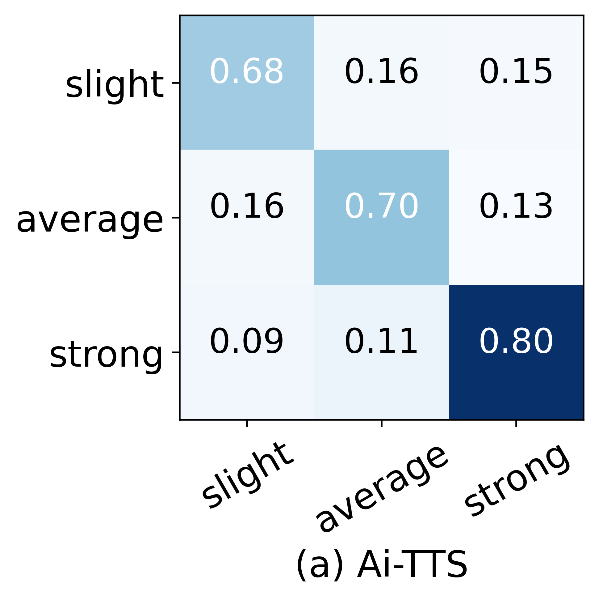
Fig. 2: Confusion matrices between perceived and intended accent intensity categories of synthesized speech. (a) Ai-TTS; b) DAW. The X-axis and Y-axis of the figures represent the perceived and intended category, namely slight, average, and strong.

We first conduct an accent intensity classification experiment. Specifically, for DAW, we follow [1] and set the adversarial weight from 0 to 0.1. We consider the weight value from 0 to 0.03 as ‘slight’, 0.04 to 0.06 as ‘average’ and 0.07 to 0.1 as ‘strong’ in three categories. For Ai-TTS, we consider the intensity scores from 0 to 0.3 as ‘slight’, 0.4 to 0.6 as ‘average’ and 0.7 to 1 as ‘strong’. We select 100 utterances from the test set, resulting in 100 samples for both systems. Accordingly, all listeners are instructed to rate the accent intensity category, that are ‘slight’, ‘average’ or ‘strong’, for each sample. A listener can listen to the samples multiple times when needed.

Fig. 2 reports the intensity confusion matrices. We can find that the Ai-TTS system shows a higher correlation between the perceived and intended accent intensity categories, with a correlation of over 80%, that is considered a competitive result against other intensity-controlled studies. Furthermore, the Ai-TTS system clearly outperforms the contestant. The experiments confirm the superiority of the proposed explicit accent intensity control mechanism.

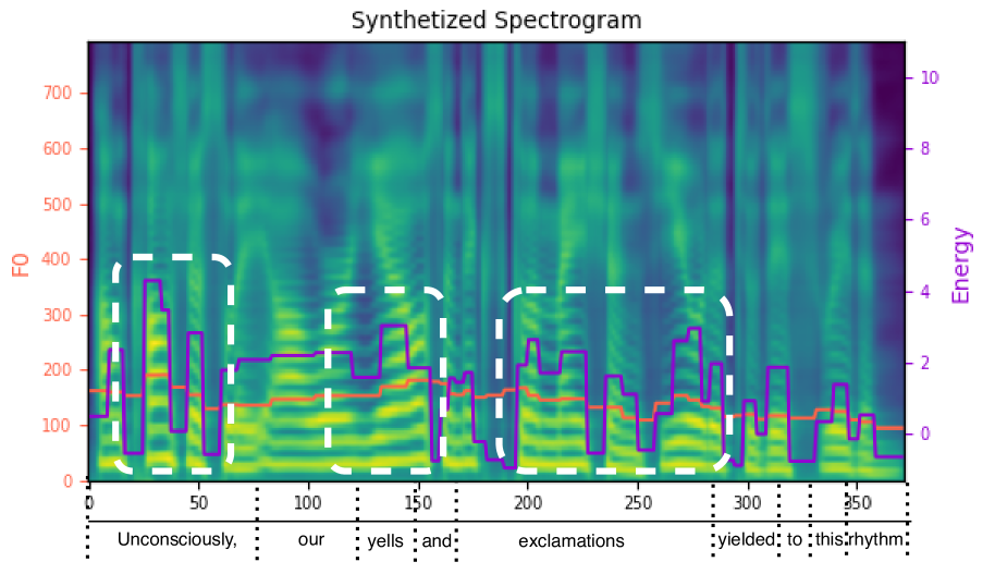
Fig. 3: Spectrogram, F0 contour and energy of an utterance with specific phoneme-level intensity score. While boxes indicates the acoustic performance with higher accent intensity. It is observed that Ai-TTS provides an effective explicit accent intensity control mechanism.

3.4 Controllability Evaluation on Phoneme-level

We further evaluate the intensity-controlled speech at phoneme level. Note that F0 (or pitch) and energy are related to accent expression [1]. Fig. 3 shows an example of spectrogram, F0 contour and energy of an utterance “Unconsciously, our yells and exclamations yielded to this rhythm.”. Due to space limit, the phoneme sequence “AH2 N K AA1 N SH AH0 S L IY0 sp AW1 ER0 Y EH1 L Z AE1 N D sp EH2 K S K L AH0 M EY1 SH AH0 N Z sp Y IY1 L D IH0 D T UW1 DH IH1 S R IH1 DH AH0 M” is omitted. We assign the intensity score of phonemes of words “Unconsciously”, “yells” and “exclamations” as 0.9 while those of other phonemes are 0.1. The white boxes in Fig. 3 show that the phonemes with higher accent intensity perform with higher F0 and energy. It indicates that fine-grained accent intensity changes can be easily detected. The Ai-TTS system provides an effective explicit accent intensity control mechanism. We suggest the readers listen to our online demos${}^{\ref{demopage}}$.

4 Conclusion

We have studied a novel TTS model, named Ai-TTS, to control the L2 accent and its intensity explicitly. We have conducted a series of experiments on utterance-and phoneme-level intensity control to validate the effectiveness of the Ai-TTS model. The proposed GoP based intensity score outperforms the adversarial weight strategy in terms of interpretability and controllability. This work marks an important step towards controllable rendering of accented TTS synthesis. In future work, we plan to further improve the intensity quantitation method.

References

- [1] Yu Zhang, Ron J Weiss, Heiga Zen, Yonghui Wu, Zhifeng Chen, RJ Skerry-Ryan, Ye Jia, Andrew Rosenberg, and Bhuvana Ramabhadran, “Learning to speak fluently in a foreign language: Multilingual speech synthesis and cross-language voice cloning,” Proc. Interspeech 2019, pp. 2080–2084, 2019.
- [2] Linsen Loots and Thomas Niesler, “Automatic conversion between pronunciations of different english accents,” Speech Communication, vol. 53, no. 1, pp. 75–84, 2011.
- [3] Christophe Veaux, Junichi Yamagishi, and Simon King, “The voice bank corpus: Design, collection and data analysis of a large regional accent speech database,” Proc. O-COCOSDA 2013, pp. 1–4, 2013.
- [4] Michael Pucher, Dietmar Schabus, Junichi Yamagishi, Friedrich Neubarth, and Volker Strom, “Modeling and interpolation of austrian german and viennese dialect in hmm-based speech synthesis,” Speech Communication, vol. 52, no. 2, pp. 164–179, 2010.
- [5] Gopala Krishna Anumanchipalli, Luis C Oliveira, and Alan W Black, “Accent group modeling for improved prosody in statistical parameteric speech synthesis,” Proc. ICASSP 2013, pp. 6890–6894, 2013.
- [6] María Luisa García Lecumberri, Roberto Barra Chicote, Rubén Pérez Ramón, Junichi Yamagishi, and Martin Cooke, “Generating segmental foreign accent,” Proc. Interspeech 2014, pp. 1303–1306, 2014.
- [7] Mohammed Waseem and CN Sujatha, “Speech synthesis system for indian accent using festvox,” International journal of Scientific Engineering and Technology Research, ISSN, pp. 2319–8885, 2014.
- [8] Sangramsing Kayte, Monica Mundada, and Dr Charansing Kayte, “Speech synthesis system for marathi accent using festvox,” International Journal of Computer Applications, vol. 130, no. 6, pp. 38–42, 2015.
- [9] Gustav Eje Henter, Jaime Lorenzo-Trueba, Xin Wang, Mariko Kondo, and Junichi Yamagishi, “Cyborg speech: Deep multilingual speech synthesis for generating segmental foreign accent with natural prosody,” Proc. ICASSP 2018, pp. 4799–4803, 2018.
- [10] Zhaoyu Liu and Brian Mak, “Multi-lingual multi-speaker text-to-speech synthesis for voice cloning with online speaker enrollment.,” Proc. Interspeech 2020, pp. 2932–2936, 2020.
- [11] Jonathan Shen, Ruoming Pang, Ron J Weiss, Mike Schuster, Navdeep Jaitly, Zongheng Yang, Zhifeng Chen, Yu Zhang, Yuxuan Wang, Rj Skerrv-Ryan, et al., “Natural tts synthesis by conditioning wavenet on mel spectrogram predictions,” Proc. ICASSP 2018, pp. 4779–4783, 2018.
- [12] Murray J Munro, Tracey M Derwing, and Susan L Morton, “The mutual intelligibility of l2 speech,” Studies in second language acquisition, vol. 28, no. 1, pp. 111–131, 2006.
- [13] Rubén Pérez-Ramón, María Luisa García Lecumberri, and Martin Cooke, “Foreign accent strength and intelligibility at the segmental level,” Speech Communication, vol. 137, pp. 70–76, 2022.
- [14] Chai Wutiwiwatchai, Ausdang Thangthai, Ananlada Chotimongkol, Chatchawarn Hansakunbuntheung, and Nattanun Thatphithakkul, “Accent level adjustment in bilingual thai-english text-to-speech synthesis,” in 2011 IEEE Workshop on Automatic Speech Recognition & Understanding. IEEE, 2011, pp. 295–299.
- [15] Yuxuan Wang, RJ Skerry-Ryan, Daisy Stanton, Yonghui Wu, Ron J Weiss, Navdeep Jaitly, Zongheng Yang, Ying Xiao, Zhifeng Chen, Samy Bengio, et al., “Tacotron: A fully end-to-end text-to-speech synthesis model,” Proc. Interspeech 2017, pp. 4006–4010, 2017.
- [16] Yi Ren, Yangjun Ruan, Xu Tan, Tao Qin, Sheng Zhao, Zhou Zhao, and Tie-Yan Liu, “Fastspeech: fast, robust and controllable text to speech,” in Proceedings of the 33rd International Conference on Neural Information Processing Systems, 2019, pp. 3171–3180.
- [17] Yi Ren, Chenxu Hu, Xu Tan, Tao Qin, Sheng Zhao, Zhou Zhao, and Tie-Yan Liu, “Fastspeech 2: Fast and high-quality end-to-end text to speech,” in International Conference on Learning Representations, 2020.
- [18] Yaroslav Ganin, Evgeniya Ustinova, Hana Ajakan, Pascal Germain, Hugo Larochelle, François Laviolette, Mario Marchand, and Victor Lempitsky, “Domain-adversarial training of neural networks,” The journal of machine learning research, vol. 17, no. 1, pp. 2096–2030, 2016.
- [19] Horacio Franco, Harry Bratt, Romain Rossier, Venkata Rao Gadde, Elizabeth Shriberg, Victor Abrash, and Kristin Precoda, “Eduspeak®: A speech recognition and pronunciation scoring toolkit for computer-aided language learning applications,” Language Testing, vol. 27, no. 3, pp. 401–418, 2010.
- [20] Longfei Yang, Jinsong Zhang, and Takahiro Shinozaki, “Self-supervised learning with multi-target contrastive coding for non-native acoustic modeling of mispronunciation verification,” Proc. Interspeech 2022, pp. 4312–4316, 2022.
- [21] Silke M Witt, “Automatic error detection in pronunciation training: Where we are and where we need to go,” in International Symposium on automatic detection on errors in pronunciation training, 2012, pp. 1–8.
- [22] Silke M Witt and Steve J Young, “Phone-level pronunciation scoring and assessment for interactive language learning,” Speech communication, vol. 30, no. 2-3, pp. 95–108, 2000.
- [23] Jungil Kong, Jaehyeon Kim, and Jaekyoung Bae, “Hifi-gan: Generative adversarial networks for efficient and high fidelity speech synthesis,” Advances in Neural Information Processing Systems, vol. 33, 2020.
- [24] Alex Waibel, “Consonant recognition by modular construction of large phonemic time-delay neural networks,” Advances in neural information processing systems, vol. 1, 1988.
- [25] Najim Dehak, Patrick J. Kenny, Réda Dehak, Pierre Dumouchel, and Pierre Ouellet, “Front-end factor analysis for speaker verification,” IEEE Transactions on Audio, Speech, and Language Processing, vol. 19, no. 4, pp. 788–798, 2011.
- [26] Vijayaditya Peddinti, Daniel Povey, and Sanjeev Khudanpur, “A time delay neural network architecture for efficient modeling of long temporal contexts,” Proc. Interspeech 2015, 2015.
- [27] Wenping Hu, Yao Qian, Frank K Soong, and Yong Wang, “Improved mispronunciation detection with deep neural network trained acoustic models and transfer learning based logistic regression classifiers,” Speech Communication, vol. 67, pp. 154–166, 2015.
- [28] Rui Liu, Berrak Sisman, Björn W. Schuller, Guanglai Gao, and Haizhou Li, “Accurate emotion strength assessment for seen and unseen speech based on data-driven deep learning,” Proc. Interspeech 2022, pp. 5493–5497, 2022.
- [29] Vassil Panayotov, Guoguo Chen, Daniel Povey, and Sanjeev Khudanpur, “Librispeech: An ASR corpus based on public domain audio books,” Proc. ICASSP 2015, pp. 5206–5210, 2015.
- [30] Guanlong Zhao, Sinem Sonsaat, Alif Silpachai, Ivana Lucic, Evgeny Chukharev-Hudilainen, John Levis, and Ricardo Gutierrez-Osuna, “L2-arctic: A non-native english speech corpus,” Proc. Interspeech 2018, pp. 2783–2787, 2018.
- [31] Diederik P Kingma and Jimmy Ba, “Adam: A method for stochastic optimization,” arXiv preprint arXiv:1412.6980, 2014.
- [32] Ashish Vaswani, Noam Shazeer, Niki Parmar, Jakob Uszkoreit, Llion Jones, Aidan N Gomez, Lukasz Kaiser, and Illia Polosukhin, “Attention is all you need,” in Advances in neural information processing systems, 2017, pp. 5998–6008.