PopArt: Efficient Sparse Regression and Experimental Design for Optimal Sparse Linear Bandits

Abstract

In sparse linear bandits, a learning agent sequentially selects an action and receive reward feedback, and the reward function depends linearly on a few coordinates of the covariates of the actions. This has applications in many real-world sequential decision making problems. In this paper, we propose a simple and computationally efficient sparse linear estimation method called PopArt that enjoys a tighter $\ell_{1}$ recovery guarantee compared to Lasso (Tibshirani, 1996) in many problems. Our bound naturally motivates an experimental design criterion that is convex and thus computationally efficient to solve. Based on our novel estimator and design criterion, we derive sparse linear bandit algorithms that enjoy improved regret upper bounds upon the state of the art (Hao et al., 2020), especially w.r.t. the geometry of the given action set. Finally, we prove a matching lower bound for sparse linear bandits in the data-poor regime, which closes the gap between upper and lower bounds in prior work.

1 Introduction

In many modern science and engineering applications, high-dimensional data naturally emerges, where the number of features significantly outnumber the number of samples. In gene microarray analysis for cancer prediction [31], for example, tens of thousands of genes expression data are measured per patient, far exceeding the number of patients. Such practical settings motivate the study of high-dimensional statistics, where certain structures of the data are exploited to make statistical inference possible. One representative example is sparse linear models [20], where we assume that a linear regression task’s underlying predictor depends only on a small subset of the input features.

On the other hand, online learning with bandit feedback, due to its practicality in many applications such as online news recommendations [26] or clinical trials [27, 42], has attracted a surge of research interests. Of particular interest is linear bandits, where in $n$ rounds, the learner repeatedly takes an action $A_{t}$ (e.g., some feature representation of a product or a medicine) from a set of available actions $\mathcal{A}\subset{\mathbb{R}}^{d}$ and receives a reward $r_{t}={\langle\theta^{*},A_{t}\rangle}+\eta_{t}$ as feedback where $\eta_{t}\in{\mathbb{R}}$ is an independent zero-mean, $\sigma$-sub-Gaussian noise. Sparsity structure is abundant in linear bandit applications: for example, customers’ interests on a product depend only on a number of its key specs; the effectiveness of a medicine only depends on a number of key medicinal properties, which means that the unknown parameter $\theta^{*}$ is sparse; i.e., it has a small number of nonzero entries.

Early studies [2, 8, 25] on sparse linear bandits have revealed that leveraging sparsity assumptions yields bandit algorithms with lower regret than those provided by full-dimensional linear bandit algorithms [3, 4, 12, 1]. However, most existing studies either rely on a particular arm set (e.g., a norm ball), which is unrealistic in many applications, or use computationally intractable algorithms. If we consider an arbitrary arm set, however, the optimal worst-case regret is ${\Theta}(\sqrt{sdn})$ where $s$ is the sparsity level of $\theta^{*}$, which means that as long as $n=O(sd)$, there exists an instance for which the algorithm suffers a linear regret [24]. This is in stark contrast to supervised learning where it is possible to enjoy nontrivial prediction error bounds for $n=o(d)$ [17]. This motivates a natural research question: Can we develop computationally efficient sparse linear bandit algorithms that allow a generic arm set yet enjoy nonvacuous bounds in the data-poor regime by exploiting problem-dependent characteristics?

The seminal work of Hao et al. [19] provides a positive answer to this question. They propose algorithms that enjoy nonvacuous regret bounds with an arbitrary arm set in the data poor regime using Lasso. Specifically, they have obtained a regret bound of $\tilde{O}({{\mathcal{C}_{\text{min}}}}^{-2/3}s^{2/3}n^{2/3})$ where ${{\mathcal{C}_{\text{min}}}}$ is an arm-set-dependent quantity. However, their work still left a few open problems. First, their regret upper bound does not match with their lower bound $\Omega({{\mathcal{C}_{\text{min}}}}^{-1/3}s^{1/3}n^{2/3})$. Second, it is not clear if ${{\mathcal{C}_{\text{min}}}}$ is the right problem-dependent constant that captures the geometry of the arm set.

	Regret Bound	Data-poor	Assumptions
Hao et al. [19]	$\tilde{O}(s^{2/3}\mathcal{C}_{\min}^{-2/3}n^{2/3})$	✓	$\mathcal{A}$ spans $\mathbb{R}^{d}$
Hao et al. [19]	${\Omega(s^{1/3}\kappa^{-2/3}n^{2/3})}$	✓	$\mathcal{A}$ spans ${\mathbb{R}}^{d}$
Algorithm 3 (Ours)	$\tilde{O}(s^{2/3}H_{*}^{2/3}n^{2/3})$	✓	$\mathcal{A}$ spans $\mathbb{R}^{d}$
Theorem 5 (Ours)	$\Omega(s^{2/3}\kappa^{-2/3}n^{2/3})$	✓	$\mathcal{A}$ spans ${\mathbb{R}}^{d}$
Hao et al. [19]	$\tilde{O}(\sqrt{\mathcal{C}_{\min}^{-1}sn})$	✗	$\mathcal{A}$ spans $\mathbb{R}^{d}$, Min. Signal
Algorithm 4 (Ours)	$\tilde{O}(\sqrt{sn})$	✗	$\mathcal{A}$ spans $\mathbb{R}^{d}$, Min. Signal

Table 1: Regret bounds of our work and the prior art where $s$, $d$, $n$ are the sparsity level, the feature dimension, and the number of rounds, respectively. The quantities $\mathcal{C}_{\min}$ and $H_{*}^{2}$ are the constants that captures the geometry of the action set (see Eq. (6) and (5)), and $\kappa$ is a parameter for a specific family of arm sets that satisfies $\kappa^{-2}=\Theta(\mathcal{C}_{\min}^{-1})=\Theta(H^{2}_{*})$. In general, $H_{*}^{2}\leq\mathcal{C}_{\min}^{-1}\leq\mathcal{C}_{\min}^{-2}$ (Propositon 2).

In this paper, we make significant progress in high-dimensional linear regression and sparse linear bandits, which resolves or partly answers the aforementioned open problems.

First (Section 3), we propose a novel and computationally efficient estimator called PopArt (POPulation covariance regression with hARd Thresholding) that enjoys a tighter $\ell_{1}$ norm recovery bound than the de facto standard sparse linear regression method Lasso in many problems. Motivated by the $\ell_{1}$ norm recovery bound of PopArt, we develop a computationally-tractable design of experiment objective for finding the sampling distribution that minimize the error bound of PopArt, which is useful in settings where we have control on the sampling distribution (such as compressed sensing). Our design of experiments results in an $\ell_{1}$ norm error bound that depends on the measurement set dependent quantity denoted by $H_{*}^{2}$ (see Eq. (5) for precise definition) that is provably better than ${{\mathcal{C}_{\text{min}}}}^{-1}$ that appears in the $\ell_{1}$ norm error bound used in Hao et al. [19], thus leading to an improved planning method for sparse linear bandits. Second (Section 4), Using PopArt, we design new algorithms for the sparse linear bandit problem, and improve the regret upper bound of prior work [19]; see Table 1 for the summary. Third (Section 5), We prove a matching lower bound in data-poor regime, showing that the regret rate obtained by our algorithm is optimal. The key insight in our lower bound is a novel application of the algorithmic symmetrization technique [34]. Unlike the conjecture of Hao et al. [19, Remark 4.5], the improvable part was not the algorithm but the lower bound for sparsity $s$.

We empirically verify our theoretical findings in Section 6 where PopArt shows a favorable performance over Lasso. Finally, we conclude our paper with future research enabled by PopArt in Section 7. Due to space constraints, we discuss related work in Appendix A but closely related studies are discussed in depth throughout the paper.

2 Problem Definition and Preliminaries

Sparse linear bandits.

We study the sparse linear bandit learning setting, where the learner is given access to an action space ${\mathcal{A}}\subset\{a\in{\mathbb{R}}^{d}\mathrel{\mathop{\mathchar 58\relax}}\|a\|_{\infty}\leq 1\}$, and repeatedly interacts with the environment as follows: at each round $t=1,\ldots,n$, the learner chooses some action $A_{t}\in\mathcal{A}$, and receives reward feedback $r_{t}={\langle\theta^{*},A_{t}\rangle}+\eta_{t}$, where ${\theta^{*}}\in{\mathbb{R}}^{d}$ is the underlying reward predictor, and ${\eta_{t}}$ is an independent zero-mean $\sigma$-subgaussian noise. We assume that $\theta^{*}$ is $s$-sparse; that is, it has at most $s$ nonzero entries. The goal of the learner is to minimize its pseudo-regret defined as

$$\operatorname{{\text{Reg}}}(n)=n\max_{a\in\mathcal{A}}{\langle\theta^{*},a\rangle}-\sum_{t=1}^{n}{\langle\theta^{*},A_{t}\rangle}.$$

Experimental design for linear regression.

In the experimental design for linear regression problem, one has a pool of unlabeled examples $\mathcal{X}$, and some underlying predictor $\theta^{*}$ to be learned. Querying the label of $x$, i.e. conducting experiment $x$, reveals a random label $y={\langle\theta^{*},x\rangle}+\eta$ associated with it, where $\eta$ is a zero mean noise random variable. The goal is to accurately estimate $\theta^{*}$, while using as few queries $x$ as possible.

Definition 1.

(Population covariance matrix $Q$) Let $\mathcal{P}({\mathcal{X}})$ be the space of probability measures over $\mathcal{X}$ with the Borel $\sigma$-algebra, and define the population covariance matrix for the distribution $\mu\in\mathcal{P}(\mathcal{X})$ as follows:

$$Q(\mu)\mathrel{\mathop{\mathchar 58\relax}}=\int_{a\in\mathcal{X}}aa^{\top}d\mu(a)$$ (1)

Classical approaches for experimental design focus on finding a distribution $\mu$ such that its induced population covariance matrix $Q(\mu)$ has properties amenable for building a low-error estimator, such as D-, A-, G-optimality [15].

Compatibility condition for Lasso.  For a positive definite matrix $\Sigma\in{\mathbb{R}}^{d\times d}$ and a sparsity level $s\in[d]\mathrel{\mathop{\mathchar 58\relax}}=\{1,\ldots,d\}$, we define its compatibility constant $\phi_{0}^{2}(\Sigma,s)$ [6] as follows:

$$\phi_{0}^{2}(\Sigma,s)\mathrel{\mathop{\mathchar 58\relax}}=\min_{S\subseteq[d]\mathrel{\mathop{\mathchar 58\relax}}|S|=s}~{}\min_{v\mathrel{\mathop{\mathchar 58\relax}}\|v_{S}\|_{1}\leq 3\|v_{-S}\|_{1}}\frac{sv^{\top}\Sigma v}{\|v_{S}\|_{1}^{2}},$$ (2)

where $v_{S}\in{\mathbb{R}}^{d}$ denotes the vector that agrees with $v$ in coordinates in $S$ and $0$ everywhere else and $v_{-S}\in{\mathbb{R}}^{d}$ denotes $v-v_{S}$.

Notation.  Let $e_{i}$ be the $i$-th canonical basis vector. We define $[x]=\{1,2,\ldots,x\}$. Let $\mathrm{supp}(\theta)$ be the set of coordinate indices $i$ where $\theta_{i}\neq 0$. We use $a\lesssim b$ to denote that there exists an absolute constant $c$ such that $a\leq cb$.

3 Improved Linear Regression and Experimental Design for Sparse Models

In this section, we discuss our novel sparse linear estimator PopArt for the setting where the population covariance matrix is known and show its strong theoretical properties. We then present a variation of PopArt called Warm-PopArt that amends a potential weakness of PopArt, followed by our novel experimental design for PopArt and discuss its merit over prior art.

PopArt (POPulation covariance regression with hARd Thresholding). Unlike typical estimators for the statistical learning setup, our main estimator PopArt described in Algorithm 1 takes the population covariance matrix denoted by $Q$ as input. We summarize our assumption for PopArt.

Assumption 1.

(Assumptions on the input of PopArt) There exists $\mu$ such that the input data points $\{(X_{t},Y_{t})\}_{t=1}^{n}$ satisfy that $X_{t}{\mathop{}\stackrel{{\scriptstyle\text{i.i.d.}}}{{\sim}}}\mathop{}\,\mu$ and $Q=Q(\mu)\mathrel{\mathop{\mathchar 58\relax}}=\operatorname{\mathbb{E}}_{X\sim\mu}[XX^{\top}]$. Furthermore, $Y_{t}={\langle\theta^{*},X_{t}\rangle}+\eta_{t}$ with $\eta_{t}$ being zero-mean $\sigma$-subgaussian noise. Also, $R_{0}\geq\max_{a\in\mathcal{A}}|\langle a,\theta^{*}-\theta_{0}\rangle|$.

Algorithm 1 PopArt (POPulation covariance regression with hARd Thresholding)

1:  Input: Samples $\{(X_{t},Y_{t})\}_{t=1}^{n}$, the population covariance matrix $Q\in{\mathbb{R}}^{d\times d}$, pilot estimator $\theta_{0}\in\mathbb{R}^{d}$, an upper bound $R_{0}$ of $\max_{a\in\mathcal{A}}|\langle a,\theta^{*}-\theta_{0}\rangle|$, failure rate $\delta$.

2:  Output: estimator $\hat{\theta}$

3:  for $t=1,\ldots,n$  do

4:     $\tilde{\theta}_{t}=Q^{-1}X_{t}(Y_{t}-\langle X_{t},\theta_{0}\rangle)+\theta_{0}$

5:  end for

6:  $\forall i\in[d],{\theta}_{i}^{\prime}=\textsf{Catoni}(\{\tilde{\theta}_{ti}\mathrel{\mathop{\mathchar 58\relax}}=\langle\tilde{\theta}_{t},e_{i}\rangle\}_{t=1}^{n},\alpha_{i},\frac{\delta}{2d})$ where $\alpha_{i}\mathrel{\mathop{\mathchar 58\relax}}=\sqrt{\frac{2\log\frac{2d}{\delta}}{n(R_{0}^{2}+\sigma^{2})(Q^{-1})_{ii}(1+\frac{2\log\frac{2d}{\delta}}{n-2\log\frac{2d}{\delta}})}}$

7:  $\hat{\theta}\leftarrow\textsf{clip}_{\lambda}({\theta^{\prime}})\mathrel{\mathop{\mathchar 58\relax}}=[{\theta}^{\prime}_{i}\operatorname{\mathds{1}}(|{\theta}^{\prime}_{i}|>\lambda_{i})]_{i=1}^{d}$ where $\lambda_{i}$ is defined in Proposition 1.

8:  return  $\hat{\theta}$

PopArt consists of several stages. In the first stage, for each $(X_{t},Y_{t})$ pair, we create a one-sample estimator $\tilde{\theta}_{t}$ (step 4). The estimator, $\tilde{\theta}_{t}$, can be viewed as a generalization of doubly-robust estimator [10, 13] for linear models. Specifically, it is the sum of two parts: one is the pilot estimator $\theta_{0}$ that is a hyperparameter of PopArt; the other is $Q(\mu)^{-1}X_{t}(Y_{t}-\langle X_{t},\theta_{0}\rangle)$, an unbiased estimator of the difference $\theta^{*}-\theta_{0}$. Thus, it is not hard to see that $\tilde{\theta}_{t}$ is an unbiased estimator of $\theta^{*}$. As we will see in Theorem 1, the variance of $\tilde{\theta}_{t}$ is smaller when $\theta_{0}$ is closer to $\theta^{*}$, showing the advantage of allowing a pilot estimator $\theta_{0}$ as input. If no good pilot estimator is available a priori, one can set $\theta_{0}=0$.

From the discussion above, it is natural to take an average of $\tilde{\theta}_{t}$. Indeed, when $n$ is large, the population covariance matrix $Q(\pi)$ is close to empirical covariance matrix $\hat{Q}\mathrel{\mathop{\mathchar 58\relax}}=\frac{1}{n}\sum_{t=1}^{n}X_{t}X_{t}^{\top}$, which makes $\hat{\theta}_{\text{avg}}\mathrel{\mathop{\mathchar 58\relax}}=\frac{1}{n}\sum_{t=1}^{n}\tilde{\theta}_{t}$ close to the ordinary least squares estimator $\hat{\theta}_{\text{OLS}}=\hat{Q}^{-1}(\frac{1}{n}\sum_{t=1}^{n}X_{t}Y_{t})$. However, for technical reasons, the concentration property of $\tilde{\theta}_{\text{avg}}$ is hard to establish. This motivates PopArt’s second stage (step 6), where, for each coordinate $i\in[d]$, we employ Catoni’s estimator [28] (see Appendix B for a recap) to obtain an intermediate estimate for each $\theta_{i}^{*}$, namely $\theta_{i}^{\prime}$.

To use Catoni’s estimator, we need to have an upper bound of the variance of $\theta_{i}^{\prime}$ for its $\alpha_{i}$ parameter. A direct calculation yields that, for all $i\in[d]$ and $t\in[n]$,

$$\textrm{Var}(\tilde{\theta}_{ti})\leq\mathinner{\left(\max_{a\in\mathcal{A}}{\langle\theta^{*}-\theta_{0},a\rangle}^{2}+\sigma^{2}\right)}\max_{i}(Q(\mu)^{-1})_{ii}$$

where $\tilde{\theta}_{ti}\mathrel{\mathop{\mathchar 58\relax}}=\langle\tilde{\theta}_{t},e_{i}\rangle$. This implies that $\mathinner{\left(R_{0}^{2}+\sigma^{2}\right)}\max_{i}(Q(\mu)^{-1})_{ii}$ is an upper bound of $\textrm{Var}(\tilde{\theta}_{ti})$. By the standard concentration inequality of Catoni’s estimator (see Lemma 1), we obtain the following estimation error guarantee for $\theta_{i}^{\prime}$; the proof can be found in Appendix C.1. Hereafter, all proofs are deferred to appendix unless noted otherwise.

Proposition 1.

Suppose Assumption 1 holds. In PopArt, for $i\in[d]$, if $n\geq 2\ln\frac{2d}{\delta}$, the following inequality holds with probability $1-\frac{\delta}{d}$:

$$|\theta_{i}^{\prime}-\theta_{i}^{*}|<\sqrt{\frac{4(R_{0}^{2}+\sigma^{2})(Q(\mu)^{-1})_{ii}^{2}}{n}\log\frac{2d}{\delta}}=\mathrel{\mathop{\mathchar 58\relax}}\lambda_{i}$$

Proposition 1 shows that, for each coordinate $i$, $(\theta_{i}^{\prime}-\lambda_{i},\theta_{i}^{\prime}+\lambda_{i})$ forms a confidence interval for $\theta_{i}^{*}$. Therefore, if $0\notin(\theta_{i}^{\prime}-\lambda_{i},\theta_{i}^{\prime}+\lambda_{i})$, we can infer that $\theta_{i}^{*}\neq 0$, i.e., $i\in\mathrm{supp}(\theta^{*})$. Based on the observation above, PopArt’s last stage (step 7) performs a hard-thresholding for each of the coordinates of $\theta^{\prime}$, using the threshold $\lambda_{i}$ for coordinate $i$. Thanks to the thresholding step, with high probability, $\hat{\theta}$’s support is contained in that of $\theta^{*}$, which means that all coordinates $i$ outside the support of $\theta^{*}$ (typically the vast majority of the coordinates when $s\ll d$) satisfy $\hat{\theta}_{i}=\theta^{*}_{i}=0$. Meanwhile, for coordinate $i$’s in $\mathrm{supp}(\theta^{*})$, the estimated value $\hat{\theta}_{i}$ is not too far from $\theta^{*}_{i}$.

The following theorem states PopArt’s estimation error bound in terms of its output $\hat{\theta}$’s $\ell_{\infty}$, $\ell_{0}$, and $\ell_{1}$ errors, respectively. We remark that replacing hard thresholding in the last stage with soft thresholding enjoys similar guarantees.

Theorem 1.

Take Assumption 1. Let $H^{2}(Q)\mathrel{\mathop{\mathchar 58\relax}}=\max_{i\in[d]}(Q^{-1})_{ii}$. Then, PopArt has the following guarantees with probability at least $1-\delta$:

1. $\forall i\in[d],|\hat{\theta}_{i}-\theta_{i}^{*}|<2\sqrt{\frac{4(R_{0}^{2}+\sigma^{2})(Q(\mu)^{-1})_{ii}}{n}\log\frac{2d}{\delta}}$ so $\|\hat{\theta}-\theta^{*}\|_{\infty}<2\sqrt{\frac{4(R_{0}^{2}+\sigma^{2})H^{2}(Q(\mu))}{n}\log\frac{2d}{\delta}},$

2. $\textrm{supp}(\hat{\theta})\subset\textrm{supp}({\theta}^{*})$ so $\|\hat{\theta}-\theta^{*}\|_{0}\leq s$,

3. $\|\hat{\theta}-\theta^{*}\|_{1}\leq 2s\sqrt{\frac{4(R_{0}^{2}+\sigma^{2})H^{2}(Q(\mu))}{n}\log\frac{2d}{\delta}}$

Interestingly, PopArt has no false positive for identifying the sparsity pattern and enjoys an $\ell_{\infty}$ error bound, which is not available from Lasso, to our knowledge. Unfortunately, a direct comparison with Lasso is nontrivial since the largest compatibility constant $\phi_{0}^{2}(\hat{\Sigma},s)$ is defined as the solution of the optimization problem (2), let alone the fact that $\phi_{0}^{2}(\hat{\Sigma},s)$ is a function of the empirical covariance matrix. While we leave further investigation as future work, our experiment results in Section 6 suggest that there might be a case where PopArt makes a meaningful improvement over Lasso.

Proof of Theorem 1.

Let $\lambda\mathrel{\mathop{\mathchar 58\relax}}=\max_{i}\lambda_{i}=\sqrt{\frac{4(R_{0}^{2}+\sigma^{2})H^{2}(Q(\mu))}{n}\log\frac{2d}{\delta}}$ From Proposition 1 and the union bound, one can check that

$$\|{\theta^{\prime}}-\theta^{*}\|_{\infty}<\lambda$$ (3)

with probability $1-\delta$. Therefore, the coordinates in $\textrm{supp}(\theta^{*})^{c}$ will be thresholded out because of $\|{\theta^{\prime}}-\theta^{*}\|_{\infty}\leq\lambda$. Therefore, (ii) holds and for all $i\in\textrm{supp}(\theta^{*})^{c}$, $|\hat{\theta}_{i}-\theta_{i}^{*}|=0$.

By definition, $\hat{\theta}=\textsf{clip}_{\lambda}({\theta^{\prime}})$, we can say that $\|\hat{\theta}-\theta^{\prime}\|_{\infty}\leq\lambda$. Plus, by Eq. (3), $\|\theta^{\prime}-\theta^{*}\|_{\infty}\leq\lambda$. By the triangle inequality, $\|\theta^{*}-\hat{\theta}\|_{\infty}\leq 2\lambda$. Therefore, (i) holds.

Lastly, (iii) can be argued as follows:

$$\|\hat{\theta}-\theta^{*}\|_{1}=\sum_{i\in[d]}|\hat{\theta}_{i}-\theta_{i}^{*}|\leq\sum_{i\in\textrm{supp}(\theta^{*})^{c}}0+\sum_{i\in\textrm{supp}(\theta^{*})}2\lambda\leq 2s\lambda.\qed$$

Warm-PopArt: Improved guarantee by warmup.  One drawback of the PopArt estimator is that its estimation error scales with $\sqrt{R_{0}^{2}+\sigma^{2}}$, which can be very large when $R_{0}$ is large. One may attempt to use the fact that PopArt allows a pilot estimator $\theta_{0}$ to address this issue since $R_{0}$ gets smaller as $\theta_{0}$ is closer to $\theta^{*}$. However, it is a priori unclear how to obtain a $\theta_{0}$ close to $\theta^{*}$ as $\theta^{*}$ is the unknown parameter that we wanted to estimate in the first place.

To get around this “chicken and egg” problem, we propose to introduce a warmup stage, which we call Warm-PopArt (Algorithm 2). Warm-PopArt consists of two stages. For the first warmup stage, the algorithm runs PopArt with the zero vector as the pilot estimator and with the first half of the samples to obtain a coarse estimator denoted by $\hat{\theta}_{0}$ which guarantees that for large enough $n_{0}$, $\|\hat{\theta}_{0}-\theta^{*}\|_{1}\leq\sigma$. In the second stage, using $\hat{\theta}_{0}$ as the pilot estimator, it runs PopArt on the remaining half of the samples.

Algorithm 2 Warm-PopArt

1:  Input: Samples $\{(X_{t},Y_{t})\}_{t=1}^{n_{0}}$, the population covariance matrix $Q\in{\mathbb{R}}^{d\times d}$, an upper bound $R_{\max}$ of $\max_{a\in\mathcal{A}}|\langle\theta^{*},a\rangle|$, number of samples $n_{0}$, failure rate $\delta$.

2:  Output: $\hat{\theta}$, an estimate of $\theta^{*}$

3:  Run $\textsc{PopArt}(\{(X_{i},Y_{i})\}_{i=1}^{\lfloor n_{0}/2\rfloor},Q,\vec{0},\delta,R_{\max})$ to obtain ${\hat{\theta}_{0}}$, a coarse estimate of $\theta^{*}$ for the next step.

4:  Run $\textsc{PopArt}(\{(X_{i},Y_{i})\}_{i=\lfloor n_{0}/2\rfloor+1}^{n_{0}},Q,\hat{\theta}_{0},\delta,\sigma)$ to obtain $\hat{\theta}$, an estimate of $\theta^{*}$.

The following corollary states the estimation error bound of the output estimator $\hat{\theta}$. Compared with PopArt’s $\ell_{1}$ recovery guarantee, Warm-PopArt’s $\ell_{1}$ recovery guarantee (Equation (4)) has no dependence on $R_{\max}$; its dependence on $R_{\max}$ only appears in the lower bound requirement for $n_{0}$.

Corollary 1.

Take Assumption 1 without the condition on $R_{0}$. Assume that $R_{\max}\geq\max_{a\in\mathcal{A}}|\langle a,\theta^{*}\rangle|$, and $n_{0}>\frac{32s^{2}(R_{\max}^{2}+\sigma^{2})H^{2}(Q(\mu))}{\sigma^{2}}\log\frac{2d}{\delta}$. Then, Warm-PopArt has, with probability at least $1-2\delta$,

$$\|\hat{\theta}-\theta^{*}\|_{1}\leq 8s\sigma\sqrt{\frac{H^{2}(Q(\mu))\ln\frac{2d}{\delta}}{n_{0}}}.$$ (4)

Remark 1.

In Algorithm 2, we choose PopArt as our coarse estimator, but we can freely change the coarse estimation step (step 3) to other principled estimation methods (such as Lasso) without affecting the main estimation error bound (4); the only change will be the lower bound requirement of $n_{0}$ to another problem-dependent constant.

Remark 2.

Warm-PopArt requires the knowledge of $R_{\max}$, an upper bound of $\max_{a\in\mathcal{A}}|\langle\theta^{*},a\rangle|$; this requirement can be relaxed by changing the last argument of the coarse estimation step (step 3) from $R_{\max}$, to some function $f(n_{0})$ such that $f(n_{0})=\omega(1)$ and $f(n_{0})=o(\sqrt{n_{0}})$ (say, $\sigma n_{0}^{\frac{1}{4}}$); with this change, a result analogous to Corollary 1 can be proved with a different lower bound requirement of $n_{0}$.

A novel and efficient experimental design for sparse linear estimation.  In the experimental design setting where the learner has freedom to design the underlying sampling distribution $\mu$, the $\ell_{1}$ error bound of PopArt and Warm-PopArt naturally motivates a design criterion. Specifically, we can choose $\mu$ that minimizes $H^{2}(Q(\mu))$, which gives the lowest estimation error guarantee. We denote the optimal value of $H^{2}(Q(\mu))$ by

$$H_{*}^{2}\mathrel{\mathop{\mathchar 58\relax}}=\underset{\mu\in\mathcal{P}(\mathcal{A})}{\textrm{min}}\max_{i\in[d]}(Q(\mu)^{-1})_{ii}~{}.$$ (5)

The minimization of $H^{2}(Q(\mu))$ is a convex optimization problem, which admits efficient methods for finding the solution. Intuitively, $H_{*}^{2}$ captures the geometry of the action set $\mathcal{A}$.

To compare with previous studies that design a sampling distribution for Lasso, we first review the standard $\ell_{1}$ error bound of Lasso.

Theorem 2.

(Buhlmann and van de Geer [6, Theorem 6.1]) With probability at least $1-2\delta$, the $\ell_{1}$-estimation error of the optimal Lasso solution $\hat{\theta}_{{\text{Lasso}}}$ [6, Eq. (2.2)] with $\lambda=\sqrt{2\log(2d/\delta)/n}$ satisfies

$$\|\hat{\theta}_{{\text{Lasso}}}-\theta^{*}\|_{1}\leq\frac{s\sigma}{\phi_{0}^{2}(\hat{\Sigma},s)}\sqrt{\frac{2\log(2d/\delta)}{n}},$$

where $\phi_{0}(\hat{\Sigma},s)^{2}$ is the compatibility constant with respect to the empirical covariance matrix $\hat{\Sigma}=\frac{1}{n}\sum_{t=1}^{n}X_{t}X_{t}^{\top}$ and the sparsity $s$ in Eq. (2).

Ideally, for Lasso, experiment design which minimizes the compatibility constant will guarantee the best estimation error bound within a fixed number of samples $n$. However, naively, the computation of the compatibility constant is intractable since Eq. (2) is a combinatorial optimization problem which is usually difficult to compute. One simple approach taken by Hao et al. [19] is to use the following computationally tractable surrogate of $\phi_{0}^{2}(\hat{\Sigma},s)$:

$$\mathcal{C}_{\min}(\mathcal{A})\mathrel{\mathop{\mathchar 58\relax}}=\underset{\mu\in\mathcal{P}(\mathcal{A})}{\textrm{max}}\lambda_{{\text{min}}}(Q(\mu))$$ (6)

where $\lambda_{{\text{min}}}(A)$ denotes the minimum eigenvalue of a matrix $A$. With the choice of sampling distribution $\mu=\underset{\mu\in\mathcal{P}(\mathcal{A})}{\textrm{argmax}}\lambda_{{\text{min}}}(Q(\mu))$, and $n\geq\tilde{\Omega}(\frac{s\cdot\mathrm{polylog}(d)}{{{\mathcal{C}_{\text{min}}}}^{2}})$, with high probability, $\phi_{0}^{2}(\hat{\Sigma},s)\geq{\mathcal{C}_{\text{min}}}/2$ holds [33, Theorem 1.8], and one can replace $\phi_{0}(\hat{\Sigma},s)$ to ${{\mathcal{C}_{\text{min}}}}/2$ in Theorem 2 to get the following corollary:

Corollary 2.

With probability at least $1-\exp(-cn)-2\delta$ for some universal constant $c$, the $\ell_{1}$-estimation error of the optimal Lasso solution $\hat{\theta}_{{\text{Lasso}}}$ satisfies

$$\|\hat{\theta}_{{\text{Lasso}}}-\theta^{*}\|_{1}\leq\frac{2s\sigma}{{{\mathcal{C}_{\text{min}}}}}\sqrt{\frac{2\log(2d/\delta)}{n}},$$ (7)

The following proposition shows that our estimator has a better error bound compared to the surrogate experimental design for Lasso of Hao et al. [19].

Proposition 2.

We have $H_{*}^{2}\leq\mathcal{C}_{\min}^{-1}\leq dH_{*}^{2}$. Furthermore, there exist arm sets for which either of the inequalities is tight up to a constant factor.

Therefore, our new estimator has $\ell_{1}$ error guarantees at least a factor $\mathcal{C}_{\min}^{-1/2}$ better than that provided by [19], as follows: when we choose the $\mu$ as the solution of the Eq. (5), then

$$(\text{RHS of \eqref{eqn:warm-popart-l1}})\lesssim s\sigma H_{*}\sqrt{\frac{\ln(2d/\delta)}{n}}\lesssim s\sigma{{\mathcal{C}_{\text{min}}}}^{-1/2}\sqrt{\frac{\ln(2d/\delta)}{n}}\lesssim s\sigma{{\mathcal{C}_{\text{min}}}}^{-1}\sqrt{\frac{\ln(2d/\delta)}{n}}\lesssim(\text{RHS of \eqref{eqn:lasso with Cmin}})$$

In addition, we also prove that there exists a case where our estimator has an $d/s$-order better error bound compared to the traditional lasso bound in Theorem 2, although this is not in terms of the compatibility constant of the empirical covariance matrix $\hat{\Sigma}$.

Proposition 3.

There exists an action set $\mathcal{A}$ and an absolute constant $C_{1}>0$ such that

$$H_{*}<C_{1}\frac{s}{d}\times\frac{1}{\phi_{0}^{2}(\Sigma,s)}$$

For the detailed proof about Proposition 2 and Proposition 3, see Section D in Appendix.

4 Improved Sparse Linear Bandits using Warm-PopArt

We now apply our new Warm-PopArt sparse estimation algorithm to design new sparse linear bandit algorithms. Following prior work [19], we adopt the classical Explore-then-Commit (ETC) framework for algorithm design, and use PopArt with experimental design to perform exploration. As we will see, the tighter $\ell_{1}$ estimation error bound of our PopArt-based estimators helps us obtain an improved regret bound.

Algorithm 3 Explore then commit with Warm-PopArt

1:  Input: time horizon $n$, action set $\mathcal{A}$, warm-up exploration length $n_{0}$, failure rate $\delta$, reward threshold parameter $R_{\max}$, an upper bound of $\max_{a\in\mathcal{A}}|\langle\theta^{*},a\rangle|$.

2:  Solve the optimization problem in Eq. (5) and denote the solution as $\mu_{*}$

3:  for $t=1,\ldots,n_{0}$ do

4:     Independently pull the arm $A_{t}$ according to $\mu_{*}$ and receives the reward $r_{t}$

5:  end for

6:  Run $\textsc{Warm-PopArt}(\{A_{t}\}_{t=1}^{n_{0}},\{r_{t}\}_{t=1}^{n_{0}},Q(\mu_{*}),\delta,R_{\max})$ to obtain $\hat{\theta}$, an estimate of $\theta^{*}$.

7:  for $t=n_{0}+1,\ldots,n$ do

8:     Take action $A_{t}=\operatorname*{arg~{}max}_{a\in\mathcal{A}}{\langle\hat{\theta},a\rangle}$, receive reward $r_{t}={\langle\theta^{*},A_{t}\rangle}+\eta_{t}$

9:  end for

Sparse linear bandit with Warm-PopArt.  Our first new algorithm, Explore then Commit with Warm-PopArt (Algorithm 3), proceeds as follows. For the exploration stage, which consists of the first $n_{0}$ rounds, it solves the optimization problem (5) to find $\mu_{*}$, the optimal sampling distribution for PopArt and samples from it to collect a dataset for the estimation of $\theta^{*}$. Then, we use this dataset to compute the Warm-PopArt estimator $\hat{\theta}$. Finally, in the commit stage, which consists of the remaining $n-n_{0}$ rounds, we take the greedy action with respect to $\hat{\theta}$. We prove the following regret guarantee of Algorithm 3:

Theorem 3.

If Algorithm 3 has input time horizon $n>16\sqrt{2}\frac{R_{\max}(R_{\max}^{2}+\sigma^{2})^{3/2}H_{*}^{2}s^{2}}{\sigma^{4}}\log\frac{2d}{\delta}$, action set $\mathcal{A}\subset[-1,+1]^{d}$, and exploration length $n_{0}=4(s^{2}\sigma^{2}H_{*}^{2}n^{2}\log\frac{2d}{\delta}R_{\max}^{-2})^{\frac{1}{3}}$, $\lambda_{1}=4\sigma\sqrt{\frac{H_{*}^{2}}{n_{0}}\log\frac{2d}{\delta}}$, then with probability at least $1-2\delta$, $\operatorname{{\text{Reg}}}(n)\leq 8R_{\max}^{1/3}(s^{2}\sigma^{2}H_{*}^{2}n^{2}\log\frac{2d}{\delta})^{\frac{1}{3}}$.

Proof.

From Corollary 1, $\|\hat{\theta}-\theta^{*}\|_{1}\leq 2s\lambda_{1}$ with probability at least $1-2\delta$. Therefore, with probability $1-2\delta$,

$$\textrm{Reg}(n) \leq R_{\max}n_{0}+(n-n_{0})\|\hat{\theta}-\theta^{*}\|_{1}\leq R_{\max}n_{0}+2sn\lambda_{1}=R_{\max}n_{0}+8sn\sigma\sqrt{\frac{H_{*}^{2}}{n_{0}}\log\frac{2d}{\delta}}$$

and optimizing the right hand side with respect to $n_{0}$ leads to the desired upper bound. ∎

Compared with Hao et al. [19]’s regret bound $\tilde{O}((R_{\max}s^{2}\sigma^{2}{{\mathcal{C}_{\text{min}}}}^{-2}n^{2})^{1/3})$ , Algorithm 3’s regret bound $\tilde{O}((R_{\max}s^{2}\sigma^{2}H_{*}^{2}n^{2})^{1/3})$ is at most $\tilde{O}((R_{\max}s^{2}\sigma^{2}{{\mathcal{C}_{\text{min}}}}^{-1}n^{2})^{1/3})$, which is at least a factor ${{\mathcal{C}_{\text{min}}}}^{\frac{1}{3}}$ smaller. As we will see in Section 5, we show that the regret upper bound provided by Theorem 3 is unimprovable in general, answering an open question of [19].

Improved upper bound with minimum signal condition.  Our second new algorithm, Algorithm 4, similarly uses Warm-PopArt under an additional minimum signal condition.

Assumption 2 (Minimum signal).

There exists a known lower bound $m>0$ such that $\min_{j\in\textrm{supp}(\theta^{*})}|\theta_{j}^{*}|>m$.

At a high level, Algorithm 4 uses the first $n_{2}$ rounds for identifying the support of $\theta^{*}$; the $\ell_{\infty}$ recovery guarantee of Warm-PopArt makes it suitable for this task. Under the minimal signal condition and a large enough $n_{2}$, it is guaranteed that $\hat{\theta}_{2}$’s support equals exactly the support of $\theta^{*}$. After identifying the support of $\theta^{*}$, Algorithm 4 treats this as a $s$-dimensional linear bandit problem by discarding the remaining $d-s$ coordinates of the arm covariates, and perform phase elimination algorithm [24, Section 22.1] therein. The following theorem provides a regret upper bound of Algorithm 4.

Algorithm 4 Restricted phase elimination with Warm-PopArt

1:  Input: time horizon $n$, finite action set $\mathcal{A}$, minimum signal $m$, failure rate $\delta$, reward threshold parameter $R_{\max}$, an upper bound of $\max_{a\in\mathcal{A}}|\langle\theta^{*},a\rangle|$

2:  Solve the optimization problem in Eq. 5 and denote the solutions as $Q$ and $\mu_{*}$, respectively.

3:  Let $n_{2}=\max(\frac{256\sigma^{2}H_{*}^{2}}{m^{2}}\log\frac{2d}{\delta},\frac{32s^{2}(R_{\max}^{2}+\sigma^{2})H_{*}^{2}}{\sigma^{2}}\log\frac{2d}{\delta})$

4:  for $t=1,\ldots,n_{2}$ do

5:     Independently pull the arm $A_{t}$ according to $\mu_{*}$ and receives the reward $r_{t}$

6:  end for

7:  $\hat{\theta}_{2}=\textsc{Warm-PopArt}(\{A_{t}\}_{t=1}^{n},\{R_{t}\}_{t=1}^{n},Q,\delta,R_{\max})$

8:  Identify the support $\hat{S}=\mathrm{supp}(\hat{\theta}_{2})$

9:  for $t=n_{2}+1,\ldots,n$ do

10:     Invoke phased elimination algorithm for linear bandits on $\hat{S}$

11:  end for

Theorem 4.

If Algorithm 4 has input time horizon $n>\max(\frac{2^{8}\sigma^{2}H_{*}^{2}}{m^{2}},\frac{2^{5}s^{2}(R_{\max}^{2}+\sigma^{2})H_{*}^{2}}{\sigma^{2}})\log\frac{2d}{\delta}$, action set $\mathcal{A}\subset[-1,1]^{d}$, upper bound of the reward $R_{\max}$, then with probability at least $1-2\delta$, the following regret upper bound of the Algorithm 4 holds: for universal constant $C>0$,

$$\textrm{Reg}(n)\leq\max(\frac{2^{8}\sigma^{2}H_{*}^{2}}{m^{2}}\log\frac{2d}{\delta},\frac{2^{5}s^{2}(R_{\max}^{2}+\sigma^{2})H_{*}^{2}}{\sigma^{2}}\log\frac{2d}{\delta})+C\sigma\sqrt{sn\log(|\mathcal{A}|n)}$$

For sufficiently large $n$, the second term dominates, and we obtain an $O(\sqrt{sn})$ regret upper bound. Theorem 4 provides two major improvements compared to Hao et al. [19, Algorithm 2]. First, when $m$ is moderately small (so that the first subterm in the first term dominates), it shortens the length of the exploration phase $n_{2}$ by a factor of $s\cdot\frac{{{\mathcal{C}_{\text{min}}}}}{H_{*}^{2}}$. Second, compared with the regret bound $\tilde{O}(\sqrt{\frac{9\lambda_{\max}(\sum_{i=1}^{n_{2}}A_{i}A_{i}^{\top}/n_{2})}{\mathcal{C}_{\min}}}\sqrt{sn})$ provided by [19], our main regret term $\tilde{O}(\sqrt{sn})$ is more interpretable and can be much lower.

5 Matching lower bound

We show the following theorem that establishes the optimality of Algorithm 3. This solves the open problem of Hao et al. [19, Remark 4.5] on the optimal order of regret in terms of sparsity and action set geometry in sparse linear bandits.

Theorem 5.

For any algorithm, any $s,d,\kappa$ that satisfies $s>2000,\kappa\in(0,1),n>8\kappa s^{2}$ and $d\geq\max(n^{1/3}s^{4/3}\kappa^{-4/3},(s+1)^{2})$, there exists a linear bandit environment an action set $\mathcal{A}$ and a $s$-sparse $\theta\in{\mathbb{R}}^{d}$, such that $\mathcal{C}_{\min}^{-1}\leq\kappa^{-2}$, $R_{\max}\leq 2$, $\sigma=1$, and

$$\textrm{Reg}_{n}\geq\Omega(\kappa^{-2/3}s^{2/3}n^{2/3})~{}.$$

We give an overview of our lower bound proof techniques, and defer the details to Appendix F.

Change of measure technique. 

Generally, researchers prove the lower bound by comparing two instances based on the information theory inequalities, such as Pinsker’s inequality, or Bregtanolle-Huber inequality. In this proof, we also use two instances $\theta$ and $\theta^{\prime}$, but we use the change of measure technique, to help lower bound the probability of events more freely. Specifically, for any event $A$,

$$\operatorname{\mathbb{P}}_{\theta}(A)=\operatorname{\mathbb{E}}_{\theta}[\operatorname{\mathds{1}}_{A}]=\operatorname{\mathbb{E}}_{\theta^{\prime}}\mathinner{\left[\operatorname{\mathds{1}}_{A}\prod_{t=1}^{n}\frac{p_{\theta}(r_{t}|a_{t})}{p_{\theta^{\prime}}(r_{t}|a_{t})}\right]}\gtrsim\operatorname{\mathbb{E}}_{\theta^{\prime}}\mathinner{\left[\operatorname{\mathds{1}}_{A}\exp\mathinner{\left(-\sum_{t=1}^{n}\langle A_{t},\theta-\theta^{\prime}\rangle^{2}\right)}\right]}~{}.$$ (8)

Symmetrization. 

We utilize the algorithmic symmetrization technique of Simchowitz et al. [34], Stoltz et al. [37], which makes it suffice to focus on proving lower bounds against symmetric algorithms.

Definition 2 (Symmetric Algorithm).

An algorithm Alg is symmetric if for any permutation $\pi\in\textit{Sym}(d)$, $\theta\in\mathbb{R}^{d}$, $\{a_{t}\}_{t=1}^{n}\in\mathcal{A}^{n}$,

$$\operatorname{\mathbb{P}}_{\theta,\textsf{Alg}}(A_{1}=a_{1},\cdots,A_{n}=a_{n})=\operatorname{\mathbb{P}}_{{\pi}(\theta),\textsf{Alg}}(A_{1}=\pi(a_{1}),\cdots,A_{n}=\pi(a_{n}))$$

where for vector $v$, $\pi(v)\in{\mathbb{R}}^{d}$ denotes its permuted version that moves $v_{i}$ to the $\pi(i)$-th position.

This approach can help us to exploit the symmetry of $\theta^{\prime}$ to lower bound the right hand side of (8); below, $\Pi\mathrel{\mathop{\mathchar 58\relax}}=\mathinner{\left\{\pi^{\prime}\mathrel{\mathop{\mathchar 58\relax}}\pi(\theta^{\prime})=\theta^{\prime}\right\}}$ is the set of permutations that keep $\theta^{\prime}$ invariant, and $A$ is an event invariant under $\Pi$:

$$\text{~{}\eqref{eqn:change-of-measure}}\geq\frac{1}{|\Pi|}\sum_{\pi\in\Pi}\operatorname{\mathbb{E}}_{\theta^{\prime}}\mathinner{\left[\operatorname{\mathds{1}}_{A}\exp(-\sum_{t=1}^{n}\langle\pi^{-1}(A_{t}),\theta-\theta^{\prime}\rangle^{2})\right]}\geq\operatorname{\mathbb{E}}_{\theta^{\prime}}\mathinner{\left[\operatorname{\mathds{1}}_{A}\exp\mathinner{\left(-\sum_{t=1}^{n}\frac{1}{|\Pi|}\sum_{\pi\in\Pi}\langle\pi^{-1}(A_{t}),\theta-\theta^{\prime}\rangle^{2}\right)}\right]}$$

which helps us use combinatorial tools over the actions for the lower bound proof.

6 Experimental results

We evaluate the empirical performance of PopArt and our proposed experimental design, along with its impact on sparse linear bandits. One can check our code from here: https://github.com/jajajang/sparse.

Case 1	Case 2

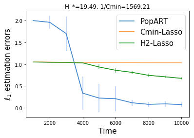
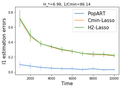
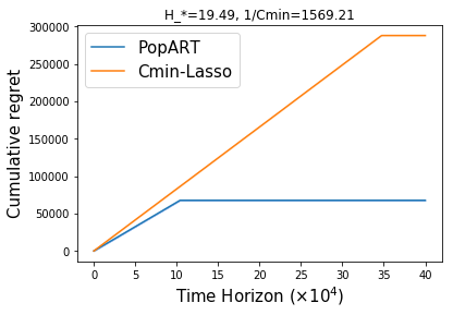
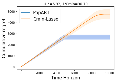
Figure 1: Experiment results on $\ell_{1}$ estimation error cumulative regret.

For sparse linear regression and experimental design, we compare our algorithm PopArt with $\mu$ being the solution of (5) with two baselines. The first baseline denoted by $C_{\min}$-Lasso is the method proposed by Hao et al. [19] that uses Lasso with sampling distribution $\mu$ defined by (6). The second baseline is $H^{2}$-Lasso, uses Lasso with sampling distribution $\mu$ defined by (5), which is meant to observe if Lasso can perform better with our experimental design and to see how PopArt is compared with Lasso as an estimator since they are given the same data. Of course, this experimental design is favored towards PopArt as we have optimized the design for it, so our intention is to observe if there ever exists a case where PopArt works better than Lasso.

For sparse linear bandits, we run a variant of our Algorithm 3 that uses Warm-PopArt in place of PopArt for simplicity. As a baseline, we use ESTC [19]. For both methods, we use the exploration length prescribed by theory. We consider two cases:

• Case 1: Hard instance where $H_{*}^{2}\ll\mathcal{C}_{\min}^{-1}$.  We use the action set constructed in Appendix D.2 where $H_{*}^{2}$ and $\mathcal{C}_{\min}$ shows a gap of $\Theta(d)$. We choose $d=10$, $s=2$, $\sigma=0.1$.

• Case 2. General unit vectors.  In this case, we choose $d=30$, $s=2$, $\sigma=0.1$ and the action set $\mathcal{A}$ consists of $|\mathcal{A}|=3d=90$ uniformly random vectors on the unit sphere.

We run each method 30 times and report the average and standard deviation of the $\ell_{1}$ estimation error and the cumulative regret in Figure 1.

Observation.

As we expected from the theoretical analysis, our estimator and bandit algorithm outperform the baselines. In terms of the $\ell_{1}$ error, for both cases, we see that PopArt converges much faster than ${{\mathcal{C}_{\text{min}}}}$-Lasso for large enough $n$. Interestingly, $H^{2}$-Lasso also improves by just using the design computed for PopArt in case 1. At the same time, $H^{2}$-Lasso is inferior than PopArt even if they are given the same data points. While the design was optimized for PopArt and PopArt has the benefit of using the population covariance, which is unfair, it is still interesting to observe a significant gap between PopArt and Lasso. For sparse linear bandit experiments, while ESTC requires exploration time almost the total length of the time horizon, ours requires a significantly shorter exploration phase in both cases and thus suffers much lower regret.

7 Conclusion

We have proposed a novel estimator PopArt and experimental design for high-dimensional linear regression. PopArt has not only enabled accurate estimation with computational efficiency but also led to improved sparse linear bandit algorithms. Furthermore, we have closed the gap between the lower and upper regret bound on an important family of instances in the data-poor regime.

Our work opens up numerous future directions. For PopArt, we speculate that $(Q(\mu)^{-1})_{ii}$ is the statistical limit for testing whether $\theta^{*}_{i}=0$ or not – it would be a valuable investigation to prove or disprove this. We believe this will also help investigate whether the dependence on $H_{*}^{2}$ in our regret upper bound is unimprovable (note our matching lower bound is only for a particular family of instances). Furthermore, it would be interesting to investigate whether we can use PopArt without relying on the population covariance; e.g., use estimated covariance from an extra set of unlabeled data or find ways to use the empirical covariance directly. For sparse linear bandits, it would be interesting to develop an algorithm that achieves the data-poor regime optimal regret and data-rich regime optimal regret $\sqrt{sdn}$ simultaneously. Furthermore, it would be interesting to extend our result to changing arm set, which poses a great challenge in planning.

Appendix

Appendix A Related work

Sparse linear bandits.

The sparse linear bandit problem is a natural extension of sparse linear regression to the bandit setup where the goal is to enjoy low regret in the high-dimensional setting by levering the sparsity of the unknown parameter $\theta^{*}$. The first study we are aware of is Abbasi-Yadkori et al. [2] that achieves a $\tilde{O}(\sqrt{sdn})$ regret bound with a computationally intractable method, which is later shown to be optimal by Lattimore and Szepesvári [24, Section 24] yet is not computationally efficient. Since then, several approaches have been proposed. A large body of literature either assumes that the arm set is restricted to a continuous set (e.g., a norm ball)  [8, 25] or that the set of available arms at every round is drawn in a time-varying manner, and playing arms greedily still induces a ‘nice’ arm distribution such as satisfying compatibility or restricted eigenvalue conditions [5, 23, 35, 30]. These assumptions allow them to leverage existing theoretical guarantees of Lasso. In contrast, we follow Hao et al. [19] and consider arm sets that are fixed throughout the bandit game without making further assumptions about the arm set. While this setup is interesting in its own for not having restrictive assumptions, it is also an important stepping stone towards efficient bandit algorithms for the more generic yet challenging setup of changing arm sets without any distributional assumptions. Our work is a direct improvement over Hao et al. [19], in that we close the gap between upper and lower bounds on the optimal worst-case regret; we refer to Table 1 for a detailed comparison.

Sparse linear regression.

Natural attempts for solving sparse linear bandits are to turn to existing results from sparse linear regression. While best subset selection (BSS) is a straightforward approach of trying all the possible sparsity patterns that achieves good guarantees, its computational complexity is prohibitive [17]. As a computationally efficient alternative, Lasso is arguably the most popular approach for sparse linear regression for its simplicity and effectiveness [39]. However, Lasso has an inferior $\ell_{1}$ norm error bound than BSS, perhaps due to its bias [41]. Rather than turning to existing results from sparse linear regression, we propose a novel estimator, PopArt, by leveraging the fact that the setup allows us to design the sampling distribution, which allows a better $\ell_{1}$ norm error bound than Lasso except for the dependence on the range of the mean response variable.

Experimental design.

In the linear bandit field, researchers often use experimental design to get the best estimator within the limited budget [36, 38, 7, 16, 29]. Especially, there were a few attempts using the population covariance based estimator instead of the traditional empirical covariance matrix [29, 38]. However, our study is the first approach that designs the experiment for minimizing the variance of each coordinate of the estimator uniformly, to the best of our knowledge.

For experimental design for sparse linear regression, Ravi et al. [32] propose heuristic approaches that ensures the design distribution satisfy incoherence conditions and restricted isometry property (RIP). Eftekhari et al. [14] study the design of $c$-optimal experiments in sparse regression models, where the goal is to estimate ${\langle c,\theta^{*}\rangle}$ with low error for some $c\in{\mathbb{R}}^{d}$; our experimental design task can be seen as simultaneously estimating ${\langle c,\theta^{*}\rangle}$ for all $c=e_{1},\ldots,e_{d}$. Huang et al. [21] propose algorithms for optimal experimental design, tailored to minimizing the asymptotic variance of the debiased Lasso estimator [22]. In contrast, our results are based on finite-sample analyses.

In the theoretical computer science literature, a line of work on sketching also provides provably efficient compressed sensing and sparse recovery algorithms [See 18, for an overview]; however, they mostly focus on using measurements (covariates) that are in $\mathinner{\{0,1\}}^{d}$ and $\mathinner{\{-1,1\}}^{d}$, as opposed to general measurement sets in ${\mathbb{R}}^{d}$.

Regression with the population covariance matrix.

There are a few studies that consider regression with the population covariance matrix: Camilleri et al. [7] devise the novel scheme for the experimental design for the kernel bandits and obtain a new estimator called RIPS that leverages the population covariance matrix and robust mean estimator like PopArt. Mason et al. [29] solve the level set estimation problem using RIPS. Tao et al. [38] also employ a similar estimator, but they do not use robust mean estimators and result in a weaker form of error bound involving additional lower order terms. The main difference of our work from all these papers is that they do not address sparse linear models. In particular, they do not perform thresholding nor provide $l_{\infty}$ or $l_{1}$ recovery guarantees for the sparse parameter.

Appendix B Catoni’s Estimator

Definition 3 (Catoni’s estimator [9]).

For the i.i.d random variables $Z_{1},\cdots,Z_{n}$, Catoni’s mean estimator $\textrm{Catoni}(\{Z_{i}\}_{i=1}^{n},\delta,\alpha)$ with error rate $\delta$ and the weight parameter $\alpha$ is defined as the unique value $y$ which satisfies

$$\sum_{i=1}^{n}\psi(\alpha(Z_{n}-y))=0$$

where $\psi(x)\mathrel{\mathop{\mathchar 58\relax}}=\textrm{sign}(x)\log(1+|x|+x^{2}/2)$.

Lemma 1 (Catoni’s estimator guarantee [9]).

For the i.i.d random variable $X_{1},\cdots,X_{n}$ with mean $\mu$, let $\hat{\mu}$ be their Catoni’s estimator with error rate $\delta$ with the weight parameter $\alpha\mathrel{\mathop{\mathchar 58\relax}}=\sqrt{\frac{2\log\frac{1}{\delta}}{n\textrm{Var}(X_{1})(1+\frac{2\log\frac{1}{\delta}}{n-2\log\frac{1}{\delta}})}}$. Then with probability at least $1-2\delta$, the following inequality holds:

$$|\hat{\mu}-\mu|<\sqrt{\frac{2\textrm{Var}(X_{1})\log\frac{1}{\delta}}{n-\log\frac{1}{\delta}}}$$

Appendix C Proofs for PopArt and Warm-PopArt

C.1 Proof for Proposition 1

Proof.

To lighten the notation, in this proof, we write $Q=Q(\mu)$, and let $(\tilde{\theta},A,\eta)$ denote random vectors distributed identically to $(\tilde{\theta}_{1},A_{1},\eta_{1})$. First, observe that $\operatorname{\mathbb{E}}\mathinner{\left[\tilde{\theta}\right]}=\theta^{*}$. We now use the law of total variance to decompose the covariance matrix of $\tilde{\theta}$, by first conditioning on $X$:

$$\operatorname{\mathbb{E}}\mathinner{\left[(\tilde{\theta}-\theta^{*})(\tilde{\theta}-\theta^{*})^{\top}\right]}= \operatorname{\mathbb{E}}\mathinner{\left[(\operatorname{\mathbb{E}}[\tilde{\theta}\mid X]-\theta^{*})(\operatorname{\mathbb{E}}[\tilde{\theta}\mid X]-\theta^{*})^{\top}\right]}+\operatorname{\mathbb{E}}\mathinner{\left[(\tilde{\theta}-\operatorname{\mathbb{E}}[\tilde{\theta}\mid X])(\tilde{\theta}-\operatorname{\mathbb{E}}[\tilde{\theta}\mid X])^{\top}\right]}$$

For the first term,

$$\operatorname{\mathbb{E}}\mathinner{\left[(\operatorname{\mathbb{E}}[\tilde{\theta}\mid X]-\theta^{*})(\operatorname{\mathbb{E}}[\tilde{\theta}\mid X]-\theta^{*})^{\top}\right]} =\operatorname{\mathbb{E}}\mathinner{\left[(\operatorname{\mathbb{E}}[\tilde{\theta}\mid X]-\theta_{0})(\operatorname{\mathbb{E}}[\tilde{\theta}\mid X]-\theta_{0})^{\top}\right]}-(\theta^{*}-\theta_{0})(\theta^{*}-\theta_{0})^{\top}$$

$$\preceq \operatorname{\mathbb{E}}\mathinner{\left[(\operatorname{\mathbb{E}}[\tilde{\theta}\mid X]-\theta_{0})(\operatorname{\mathbb{E}}[\tilde{\theta}\mid X]-\theta_{0})^{\top}\right]}$$

$$= \operatorname{\mathbb{E}}\mathinner{\left[Q^{-1}X(X^{\top}(\theta^{*}-\theta_{0}))^{2}X^{\top}Q^{-1}\right]}$$

$$\preceq R_{0}^{2}\operatorname{\mathbb{E}}\mathinner{\left[Q^{-1}XX^{\top}Q^{-1}\right]}=R_{0}^{2}Q^{-1}$$

For the second term,

$$\operatorname{\mathbb{E}}\mathinner{\left[(\tilde{\theta}-\operatorname{\mathbb{E}}[\tilde{\theta}\mid X])(\tilde{\theta}-\operatorname{\mathbb{E}}[\tilde{\theta}\mid X])^{\top}\right]}=\operatorname{\mathbb{E}}[Q^{-1}XX^{\top}Q^{-1}\eta^{2}]=\sigma^{2}Q^{-1}.$$

Combining the above two bounds, we have $\textrm{Var}(\tilde{\theta})=\operatorname{\mathbb{E}}\mathinner{\left[(\tilde{\theta}-\theta^{*})(\tilde{\theta}-\theta^{*})^{\top}\right]}\preceq(R_{0}^{2}+\sigma^{2})Q^{-1}$. Therefore, we can bound $\textrm{Var}(\tilde{\theta}_{i})$ as follows:

$$\textrm{Var}(\tilde{\theta}_{i}) =\operatorname{\mathbb{E}}[(e_{i}^{\top}(\tilde{\theta}-\theta^{*}))^{2}]\leq(R_{0}^{2}+\sigma^{2})(Q^{-1})_{ii}$$

By the theoretical guarantee of the Catoni’s estimator (Lemma 1 in the Appendix), the desired inequality holds. ∎

C.2 Full version of Corollary 1 and its proof

Corollary 3.

If Warm-PopArt receives inputs $\mathinner{\left\{X_{t},Y_{t}\right\}}_{t=1}^{n_{0}}$ drawn from $\mu$, $Q(\mu)$, failure probability $\delta$, and $R_{\max}$ such that $R_{\max}\geq\max_{a\in\mathcal{A}}|\langle a,\theta^{*}\rangle|$, and $n_{0}>\frac{32s^{2}(R_{\max}^{2}+\sigma^{2})H^{2}(Q(\mu))}{\sigma^{2}}\log\frac{2d}{\delta}$, then all the following items hold with probability at least $1-2\delta$:

1. $\|\hat{\theta}-\theta^{*}\|_{\infty}\leq 8\sigma H(Q)\sqrt{\frac{\ln\frac{2d}{\delta}}{n_{0}}}$

2. $\textrm{supp}(\hat{\theta})\subset\textrm{supp}({\theta}^{*})$ so $\|\hat{\theta}-\theta^{*}\|_{0}\leq s$

3. $\|\hat{\theta}-\theta^{*}\|_{1}\leq 8s\sigma H(Q)\sqrt{\frac{\ln\frac{2d}{\delta}}{n_{0}}}$

Proof.

Since $n_{0}$ is sufficiently large, from the Theorem 1 with $R_{0}=R_{\max}$ we can say that $\|\theta_{0}-\theta^{*}\|_{1}\leq\sigma$ with probability $1-\delta$. Applying Theorem 1 again with $R_{0}=\sigma$ we can get all (i), (ii), (iii) directly with probability $1-\delta$. The corollary follows from a union bound. ∎

Appendix D Proof of Proposition 2 and Proposition 3

First, we will prove

$$H_{*}^{2}\leq\mathcal{C}_{\min}^{-1}\leq dH_{*}^{2}.$$ (9)

For each of the two inequalities, We will give a tight example in the next subsection.

Proof.

For any positive definite matrix $Q\in{\mathbb{R}}^{d\times d}$,

$$H^{2}(Q)=\max_{i\in[d]}(Q^{-1})_{ii}=\max_{i\in[d]}e_{i}^{\top}Q^{-1}e_{i}\leq\max_{v\in\mathbb{S}^{d-1}}v^{\top}Q^{-1}v=\lambda_{\max}(Q^{-1})\leq\mathsf{tr}(Q^{-1})\leq dH^{2}(Q)$$ (10)

Now, let the solution of the Eq. (5) and Eq. (6) as $\mu_{H}$ and $\mu_{C}$, respectively. Then, by the rightmost inequality of (10) we have

$$\frac{1}{\mathcal{C}_{\min}}=\lambda_{\max}(Q(\mu_{C})^{-1})\leq\lambda_{\max}(Q(\mu_{H})^{-1})\leq dH_{*}^{2}$$

and by the leftmost inequality of the (10) we have

$$H_{*}^{2}\leq H^{2}(Q(\mu_{C}))\leq\lambda_{\max}(Q(\mu_{C})^{-1})=\frac{1}{\mathcal{C}_{\min}}$$

Therefore, the inequality part of the Proposition 2 holds. ∎

D.1 First equality condition analysis of Eq. (9)

For the case when $\mathcal{C}_{\min}^{-1}=\Theta(H_{*}^{2})$, consider $\mathcal{A}=\{e_{i}|i=1,\cdots,d\}$; it can be seen that $H_{*}^{2}=\mathcal{C}_{\min}^{-1}=d$.

D.2 Second equality condition analysis of Eq. (9)

For the case when $\mathcal{C}_{\min}^{-1}=\Theta(dH_{*}^{2})$, consider $\mathcal{A}=\mathinner{\left\{a_{1},\ldots,a_{d}\right\}}$, where

$$a_{1}= \frac{1}{\sqrt{d}}e_{1}$$

$$a_{i}= e_{1}+\frac{1}{\sqrt{d}}e_{i}.$$

and we will calculate $H^{2}(Q(\pi))$ and $\lambda_{\min}(Q(\pi))$ for the optimal sampling distributions $\pi$ to achieve $H^{2}_{*}$ and $\mathcal{C}_{\min}$, respectively.

D.2.1 Prove that the optimal $\pi$ satisfies $\pi(a_{2})=\pi(a_{3})=\cdots=\pi(a_{d})$

We will first show that for both objectives $H^{2}(Q(\pi))$ and $\lambda_{\min}(Q(\pi))$, there exists an optimal sampling distribution $\pi$ such that $\pi(a_{2})=\pi(a_{3})=\cdots=\pi(a_{d})$.

Denote by $a\mathrel{\mathop{\mathchar 58\relax}}=\pi(a_{1})$. Fix $a$. For notational convenience, let $\pi(a_{i})\mathrel{\mathop{\mathchar 58\relax}}=b_{i}$ and $\mathbb{b}=(b_{2},b_{3},\cdots,b_{d})\in\mathbb{R}^{d-1}$.

For $H^{2}(Q(\pi))$:

Then the covariance matrix $Q(\pi)$ (abbreviated as $Q$) has the following form:

$$Q=\begin{bmatrix}\frac{a}{d}+\sum b_{i}&\frac{b_{2}}{\sqrt{d}}&\cdots&\frac{b_{d}}{\sqrt{d}}\\ \frac{b_{2}}{\sqrt{d}}&&&\\ \vdots&&\frac{1}{d}\mathrm{diag}(\mathbb{b})&\\ \frac{b_{d}}{\sqrt{d}}&&&\end{bmatrix}$$ (11)

After some calculation, one can get the determinant

$$\mbox{det}(Q)=\frac{a(\Pi_{i=2}^{d}b_{i})}{d^{d}}$$

and the cofactor

$$C_{ii}=\begin{cases}(\frac{\Pi_{i=1}^{d}b_{i}}{d^{d-1}})&\text{if }i=1\\ (\frac{a}{d}+b_{i})(\frac{\Pi_{s=2}^{d}b_{s}}{b_{i}d^{d-2}})&\text{if }i=2,\cdots,d\end{cases}$$

and therefore

$$(Q^{-1})_{ii}=\begin{cases}(\frac{d}{a})&\text{if }i=1\\ (\frac{a}{d}+b_{i})d^{2}/(ab_{i})&\text{if }i=2,\cdots,d\end{cases}$$

When $a$ is a fixed parameter, $(Q^{-1})_{ii}=\frac{d^{2}}{a}+\frac{d}{b_{i}}$ and therefore the $\arg\max_{i}(Q^{-1})_{ii}=\arg\min_{i}b_{i}$. Under the constraint $\sum_{i=2}^{d}b_{i}=1-a$, the optimal solution is reached when $b_{2}=b_{3}=\cdots=b_{d}$.

For $\lambda_{\min}(Q(\pi))$:

we will utilize symmetry of $\lambda_{\min}(Q(\pi))$. Note that $\lambda_{\min}(Q)$ is a concave function w.r.t $Q$. Suppose that the $({a},b_{2}^{\prime},b_{3}^{\prime},\cdots,b_{d}^{\prime})=\arg\max_{\pi}{\lambda_{\min}(Q(\pi))}$. Then from the symmetry, for any cyclic permutation $P$, all $({a},b_{P^{i}(2)}^{\prime},b_{P^{i}(3)}^{\prime},\cdots,b_{P^{i}(d)}^{\prime})$ $i=1,\cdots,d-1$ also achieves the maximum. Therefore, by Jensen’s inequality,

$${{\mathcal{C}_{\min}}}=\frac{1}{d}\sum_{i=0}^{d-1}{\lambda_{\min}(Q(a,b_{P^{i}(2)}^{\prime},b_{P^{i}(3)}^{\prime},\cdots,b_{P^{i}(d)}^{\prime}))}\leq{\lambda_{\min}(Q(a,\frac{1-a}{d-1},\frac{1-a}{d-1},\cdots,\frac{1-a}{d-1}))}$$

Therefore, $(a,\frac{1-a}{d-1},\frac{1-a}{d-1},\cdots,\frac{1-a}{d-1})$ is also a maximizer of $\lambda_{\min}(Q(\pi))$.

Therefore, from now on, consider only the strategy $\pi$ that satisfies $\pi(a_{2})=\pi(a_{3})=\cdots=\pi(a_{d})$ for this section, and let $a=\pi(a_{1})$ and $b=\pi(a_{2})$. Then $a+(d-1)b=1$. Now the covariance matrix induced by $\pi$ is of the following form:

$$Q=\begin{bmatrix}\frac{a}{d}+(d-1)b&\frac{b}{\sqrt{d}}&\cdots&\frac{b}{\sqrt{d}}\\ \frac{b}{\sqrt{d}}&&&\\ \vdots&&\frac{b}{d}I_{d-1}&\\ \frac{b}{\sqrt{d}}&&&\end{bmatrix}$$ (12)

D.2.2 Calculating $H_{*}^{2}$

One can calculate $\mbox{det}(Q)=\frac{a}{d}(\frac{b}{d})^{d-1}$ (using again the cofactor method) and the cofactor

$$C_{ii}=\begin{cases}(\frac{b}{d})^{d-1}&\text{if }i=1\\ (\frac{a}{d}+b)(\frac{b}{d})^{d-2}&\text{otherwise}\end{cases}$$

and therefore

$$(Q^{-1})_{ii}=\begin{cases}(\frac{d}{a})&\text{if }i=1\\ (\frac{a}{d}+b)d^{2}/(ab)&\text{otherwise}\end{cases}$$

For $i=2,\ldots,d$, $(Q^{-1})_{ii}$ is always larger than $(Q^{-1})_{11}$, and by taking derivatives, the $b$ that minimizes the $(Q^{-1})_{22}$ is $\sqrt{\frac{d}{d-1}}-1=\frac{1}{\sqrt{d-1}(\sqrt{d}+\sqrt{d-1})}$ , and the corresponding $(Q^{-1})_{22}=d(\sqrt{d}+\sqrt{d-1})^{2}=\Theta(d^{2})$. In this case, $a=d-\sqrt{d(d-1)}$ (close to 1/2).

D.2.3 Calculating $\mathcal{C}_{\min}$

The characteristic function of the $Q$ is

$$(\lambda^{2}-B\lambda+C)(\lambda-\frac{b}{d})^{d-2}$$

where $B=\frac{1}{d}+\frac{(d^{2}-2d+2)b}{d}>0$ and $C=\frac{b-(d-1)b^{2}}{d^{2}}>0$. Note that for equation of the form $\lambda^{2}-B\lambda+C=0$ ($B,C>0$), the smaller root is $\lambda^{*}=\frac{B-\sqrt{B^{2}-4C}}{2}=\frac{2C}{B+\sqrt{B^{2}-4C}}=\Theta(\frac{C}{B})$. This is because $B\leq B+\sqrt{B^{2}-4C}\leq 2B$.

Therefore, the smaller root of the quadratic equation $\lambda^{2}-B\lambda+C=0$ satisfies

$$\lambda^{*}=\Theta(\frac{C}{B})=\frac{(b-(d-1)b^{2})/d^{2}}{1/d+(d^{2}-2d+2)b/d}\leq\frac{b/d^{2}}{bd}\leq\frac{1}{d^{3}}.$$

D.2.4 Lower bound of $\frac{1}{\phi_{0}^{2}(Q(\pi),s)}$

It is difficult to directly calculate the compatibility constant of $Q(\pi)$, but we can bound it using the diagonal entries of $Q(\pi)$. Note that

$$\phi^{2}=\min_{S\subset[d]}\min_{v\in\mathcal{C}_{S}}\frac{sv^{\top}Qv}{\|v_{S}\|_{1}^{2}}\leq s\min_{v\in\{e_{i}\}_{i=1}^{d}}\frac{v^{\top}Qv}{1}=s\min_{i\in[d]}(Q_{ii})$$

and therefore $\frac{1}{\phi^{2}}\geq\frac{1}{\min_{i\in[d]}sQ_{ii}}$.

We will use the same notation in D.2.1: denote by $a\mathrel{\mathop{\mathchar 58\relax}}=\pi(a_{1})$ and let $\pi(a_{i})\mathrel{\mathop{\mathchar 58\relax}}=b_{i}$ and $\mathbb{b}=(b_{2},b_{3},\cdots,b_{d})\in\mathbb{R}^{d-1}$. Then the covariance matrix $Q(\pi)$ (abbreviated as $Q$) has the following form:

$$Q=\begin{bmatrix}\frac{a}{d}+\sum b_{i}&\frac{b_{2}}{\sqrt{d}}&\cdots&\frac{b_{d}}{\sqrt{d}}\\ \frac{b_{2}}{\sqrt{d}}&&&\\ \vdots&&\frac{1}{d}Diag(\mathbb{b})&\\ \frac{b_{d}}{\sqrt{d}}&&&\end{bmatrix}$$ (13)

From the basic constraint $a+\sum_{i=2}^{d}b_{i}=1$, $\min_{i\in[d]}Q_{ii}=\min_{i\in\{2,\cdots,d\}}\frac{b_{i}}{d}=O(\frac{1}{d^{2}})$. Therefore $\frac{1}{\phi^{2}}=\Omega(d^{2}/s)$. This means even for the best case of the compatibility constant cannot beat the recovery bound of PopArtfor this action set.

Appendix E Proofs for Sparse Linear Bandits

E.1 Proof of Theorem 4

Proof.

From the (i) in Corollary 3, when $n_{2}=\frac{256\sigma^{2}H_{*}^{2}}{m^{2}}\log\frac{d}{\delta}$, with probability at least $1-2\delta$,

$$\|\hat{\theta}-\theta^{*}\|_{\infty}<8\sigma\sqrt{\frac{H_{*}^{2}}{n_{2}}\log\frac{2d}{\delta}}=\frac{m}{2}$$

Therefore, with probability at least $1-2\delta$, for any index $i\in\textrm{supp}(\theta^{*})^{C}$, $\hat{\theta}_{i}=0$, and for any index $j\in\textrm{supp}(\theta^{*})$, $|\hat{\theta}_{j}|>|\theta_{j}^{*}|-\frac{m}{2}>0$. Thus, $\textrm{supp}(\theta^{*})=\textrm{supp}(\hat{\theta})$ with probability at least $1-2\delta$. After that, we use the following result about the phased elimination [24]:

Theorem 6.

(Lattimore and Szepesvári [24], Theorem 22.1) The $n$-step regret of phased elimination algorithm satisfies

$$\textrm{Reg}_{n}\leq C\sigma\sqrt{nd\log(|\mathcal{A}|n)}$$

for an appropriately chosen universal constant $C>0$.

∎

Appendix F Proof of Lower Bound

In this section, we prove Theorem 5. We start with a restatement of it.

Theorem 7.

(Restatement of the Theorem 5) For any algorithm, any $s,d,\kappa$ that satisfies $s>2000,\kappa\in(0,1),n>8\kappa s^{2},d\geq\max(n^{1/3}s^{4/3}\kappa^{-4/3},(s+1)^{2})$, there exists a linear bandit environment with an action set $\mathcal{A}$ and a $s$-sparse $\theta\in{\mathbb{R}}^{d}$, such that $\mathcal{C}_{\min}(\mathcal{A})^{-1}\leq\kappa^{-2}$, $R_{\max}\leq 2$, $\sigma=1$, and

$$\textrm{Reg}_{n}\geq\Omega(\kappa^{-2/3}s^{2/3}n^{2/3})~{}.$$

In the lower bound instance that establishes Theorem 7, we will prove that ${2\kappa^{-2}}\geq\mathcal{C}_{\min}(\mathcal{A})^{-1}\geq H_{*}^{2}$ (see Section F.3.1), and conclude that our $\tilde{O}(H_{*}^{2/3}s^{2/3}n^{2/3})$ regret upper bound of Algorithm 3 has a matching lower bound and conclude that the algorithm and the lower bound are both optimal in this setting.

For convenience, throughout the rest of this section, we prove the following slight variant of Theorem 7, where the dimensonality is $d+1$ as opposed to $d$, and the sparsity is $2s+1$ as opposed to $s$; note that the changes of these parameters do not affect the orders of the regret bounds in terms of them.

Theorem 8.

For any algorithm, any $s,d,\kappa$ that satisfies $s>1000$ and is a multiple of 4, $\kappa\in(0,1),n>8\kappa s^{2},d\geq\max(n^{1/3}s^{4/3}\kappa^{-4/3},(s+1)^{2})$, there exists a linear bandit environment an action set $\mathcal{A}$ and a $(2s+1)$-sparse $\theta\in{\mathbb{R}}^{d+1}$, such that $\mathcal{C}_{\min}(\mathcal{A})^{-1}\leq 2\kappa^{-2}$, $R_{\max}\leq 2$, $\sigma=1$, and

$$\textrm{Reg}_{n}\geq\Omega(\kappa^{-2/3}s^{2/3}n^{2/3})~{}.$$

Construction

Following the standard minimax lower bound and hypothesis testing terminology, we will often refer to an underlying reward predictor $\theta\in{\mathbb{R}}^{d+1}$ as a hypothesis. Let

$$\Theta_{s}=\Big{\{}\theta\in{\mathbb{R}}^{d+1}|\theta_{i}\in\{-\epsilon,0,\epsilon\}\text{ for }i\in[d],\theta_{d+1}=-1,\|\theta\|_{0}=s+1\Big{\}},$$

where $\epsilon=\kappa^{-2/3}s^{-1/3}n^{-1/3}$. We will use $\Theta_{s}$ and $\Theta_{2s}$ as our hypothesis space throughout the proof.

We construct a low-regret action set $\mathcal{I}$ and an informative action set ${\mathcal{H}}$ as follows:

$$\mathcal{I} =\Big{\{}x\in{\mathbb{R}}^{d+1}|x_{j}\in\{-1,0,1\}\text{ for }j\in[d],\|x\|_{0}=2s,x_{d+1}=0\Big{\}}$$

$${\mathcal{H}} =\Big{\{}x\in{\mathbb{R}}^{d+1}|x_{j}\in\{-\kappa,\kappa\}\text{ for }j\in[d],|\sum_{j=1}^{d}x_{j}|\leq{\kappa}\sqrt{2d\ln 2d},x_{d+1}=1\Big{\}}$$

where $\kappa\in(0,1)$ is a constant. The action set is the union $\mathcal{A}=\mathcal{I}\cup{\mathcal{H}}$.

Our linear bandit environment parameterized by $\theta\in{\mathbb{R}}^{d+1}$ is defined as: given action taken $A_{t}$, its reward $r_{t}={\langle\theta,A_{t}\rangle}+\eta_{t}$, where $\eta_{t}\sim N(0,1)$ is an independently drawn standard Gaussian noise. Note that by construction, $\eta_{t}$ is $\sigma^{2}$-subgaussian with $\sigma=1$.

Notations

In this section, we will use ${\boldsymbol{A}}=(A_{1},\cdots,A_{n})\in\mathcal{A}^{n}$ as the random variable about the history of actions. For ${\boldsymbol{a}}{=(a_{1},\ldots,a_{n})}\in\mathcal{A}^{n}$, let $T({\mathcal{H}};{\boldsymbol{a}})=\sum_{t=1}^{n}\operatorname{\mathds{1}}(a_{t}\in{\mathcal{H}})$, which represents the total number of pulls of arms in ${\mathcal{H}}$ in the learning process. For brevity of notation, we will write the random variable $T({\mathcal{H}};{\boldsymbol{A}})$ as $T({\mathcal{H}})$, and $\mathcal{C}_{\min}(\mathcal{A})$ as $\mathcal{C}_{\min}$ throughout this section. Let $\mathsf{Sub}_{x}=\{S\subset[d]||S|=x\}$, the set of subsets of $[d]$ which has $x$ elements. In subsequent proofs, given a bandit algorithm $\mathsf{Alg}$ and an bandit environment $\theta$, we use $\operatorname{\mathbb{P}}_{\theta,\mathsf{Alg}}$ and $\operatorname{\mathbb{E}}_{\theta,\mathsf{Alg}}$ to denote probability and expectation under the probability space induced by the interaction history between them. For any set of indices $S\subset[d+1]$, let ${\text{Sym}}(S)$ be the symmetric group of the set $S$ (i.e. the collection of all permutations over $S$), and let $\Pi_{S}=\mathinner{\left\{\sigma\in{\text{Sym}}([d+1])\mathrel{\mathop{\mathchar 58\relax}}{\sigma(j)=j\text{ for all }j\in[d+1]\backslash S}\right\}}$ be the set of permutations which permutes only the indices in $S$, and let $\Pi_{a\mathrel{\mathop{\mathchar 58\relax}}b}=\Pi_{\{a,a+1,\cdots,b\}}$.

Structure of the section

Here is the high-level idea of the proof structure.

• Reduction to symmetric algorithms using algorithmic symmetrization (Section F.1) : First, we will prove that the regret lower bound of symmetric sparse linear bandit algorithms (see Definition 8) is also the lower bound of the general sparse linear bandit algorithms (Lemma 5). Keen readers may note that our action set construction is symmetric except for the $(d+1)$-th coordinate, and this is for exploiting the symmetry. By focusing on proving lower bounds for symmetric algorithms, we can exploit the favorable combinatorial properties of our action spaces to establish tighter lower bounds.

• Count the number of mistakes (Section F.2.1): Next, we will prove the core proposition of the lower bound proof, Proposition 4. This proposition can be summarized as, ‘the learning agent has to pull a sufficiently large number of arms in ${\mathcal{H}}$ (informative actions with high regret) to make less mistakes’, where ‘mistakes’ refers to coordinates in the support of $\theta$ that has not been ‘hit’ sufficiently by the agent via pulling the low-regret arms $\mathcal{I}$ (See Equation (14) for a formal definition). This implies an inherent tension between pulling informative, high regret arms ${\mathcal{H}}$ and pulling low regret arms $\mathcal{I}$, which eventually leads to the desired lower bound in Theorem 5.

• Lower bound on symmetric algorithms (Section F.2.2) : Now it remains to show the proof of Proposition 4. Here, to improve the $\Omega(s^{1/3}n^{2/3})$ regret lower bound proved by Hao et al. [19] to $\Omega(s^{2/3}n^{2/3})$, we deviate from their usage of Bretagnolle-Huber inequality for binary hypothesis testing, and take a novel combination of various techniques such as a change of measure technique, combinatorial calculation by utilizing symmetry (Claim 1).

F.1 Algorithmic symmetrization: reducing lower bounds for general algorithms to symmetric algorithms

In this section, we show how proving a lower bound for generic algorithms can be reduced to that of permutation-symmetric (abbrev. symmetric) (augmented) algorithms (Definition 8), specifically Lemma 5. To introduce symmetric algorithms, let us first define some useful terminology. We first define a frequent coordinate set, which is the set of coordinates that are frequently ’hit’ by low-regret arm pulls ($\mathcal{I}$.)

Definition 4 (Frequent coordinate set).

Let ${\mathcal{U}({\boldsymbol{a}})}=\{U\in\mathsf{Sub}_{d/2}|\forall i\in U,\sum_{t=1}^{n}|a_{ti}|\operatorname{\mathds{1}}(a_{t}\in\mathcal{I})\geq\mathop{(d/2){\text{-}}\max}\{\sum_{t=1}^{n}|a_{tj}|\operatorname{\mathds{1}}(a_{t}\in\mathcal{I})\}_{j=1}^{d}\}$ where $\mathop{k{\text{-}}\max}S$ for a set $S\subseteq{\mathbb{R}}$ is the $k$-th largest element of $S$.

We also define coordinate-selection bandit algorithm which outputs top $d/2$-coordinates that are most frequently hit.

Definition 5.

(Coordinate-selection bandit algorithm; Coordination of an algorithm).

1. Define a coordinate-selection bandit algorithm $\mathsf{B}$ as: at time step $t$, choose action $A_{t}$ based on its historical observations $(A_{s},r_{s})_{s=1}^{t-1}$; finally it outputs $\hat{S}\in\mathcal{U}({\boldsymbol{A}})$. In other words, all elements in $\hat{S}$ are among the top $\frac{d}{2}$ most frequently chosen coordinates (including ties) when restricted to arm pull history on $\mathcal{I}$.

2. Given a bandit algorithm $\mathsf{Alg}$, define its coordination $\widetilde{\mathsf{Alg}}$ as: at time step $t$, use $\mathsf{Alg}$ to output $A_{t}$ based on all historical observations $(A_{s},r_{s})_{s=1}^{t-1}$; finally, output $\hat{S}\in\mathcal{U}({\boldsymbol{A}})$ with the lowest dictionary index. In other words, the elements in $\hat{S}$ are the top $\frac{d}{2}$ most frequently chosen coordinates when restricted to arm pull history on $\mathcal{I}$.

With this notation, for any coordinate-selection bandit algorithm, its output $\hat{S}\in\mathcal{U}({\boldsymbol{A}})$ with probability 1. As a result, we will mainly focus on $({\boldsymbol{a}},U)\in\mathcal{A}^{n}\times\mathsf{Sub}_{d/2}$ such that $U\in\mathcal{U}({\boldsymbol{a}})$, but for the lemmas we keep the generality and consider any $U\subset[d]$.

Remark 3.

From the above definitions, it can be readily seen that $\mathsf{Alg}$’s coordination, $\widetilde{\mathsf{Alg}}$, is a valid coordinate-selection bandit algorithm. However, a coordinate-selection bandit algorithm does not need to break ties in dictionary order.

Remark 4.

$\widetilde{\mathsf{Alg}}$ outputs $\hat{S}$ by breaking ties in dictionary order. While this breaks symmetry by favoring coordinates with lower indices, as we will see in our reduction proof (proof of Lemma 5), we do not require $\widetilde{\mathsf{Alg}}$ to be symmetric (we will define symmetry momentarily in Definition 8); instead, we will work on a symmetrized version of $\widetilde{\mathsf{Alg}}$ (Definition 10).

Definition 6 (Permutaion over sets of coordinates, and vectors in ${\mathbb{R}}^{d+1}$).

Given a permutation $\sigma\in\Pi_{1\mathrel{\mathop{\mathchar 58\relax}}d}$:

• For a subset of coordinates $S\subset[d]$, define $\sigma(S)\subset[d]$ as $\sigma(S)\mathrel{\mathop{\mathchar 58\relax}}=\mathinner{\left\{\sigma(i)\mathrel{\mathop{\mathchar 58\relax}}i\in S\right\}}$.

• For vector $v\in{\mathbb{R}}^{d+1}$, define $\sigma(v)=(v_{\sigma^{-1}(1)},\ldots,v_{\sigma^{-1}(d+1)})=P_{\sigma}v\in{\mathbb{R}}^{d+1}$ as the permuted version of $v$ using $\sigma$, where $P_{\sigma}=(e_{\sigma(1)},\ldots,e_{\sigma(d+1)})\in{\mathbb{R}}^{(d+1)\times(d+1)}$ is the permutation matrix induced by $\sigma$ and $e_{j}$ denotes $j$-th standard basis. Note that for every $i\in[d+1]$, $\sigma(e_{i})=e_{\sigma(i)}$.

• For sequence of actions ${\boldsymbol{a}}=(a_{1},\ldots,a_{n})\in\mathcal{A}^{n}$, define $\sigma({\boldsymbol{a}})=(\sigma(a_{1}),\ldots,\sigma(a_{n}))$ as its permuted version using $\sigma$.

Intuitively, $\sigma(\cdot)$ “moves” the $i$-th entry of input vector $v$ to the vector’s $\sigma(i)$-th coordinate. We will frequently apply the above vector permutation operation in our subsequent proofs, where the vector $v\in{\mathbb{R}}^{d+1}$ are often taken as actions $A_{t}$ or hypotheses (underlying reward predictors) $\theta$.

Definition 7 (Permutation-invariant action space).

An action space $\mathcal{A}$ is said to be permutation-invariant, if for any $\pi\in\Pi_{1\mathrel{\mathop{\mathchar 58\relax}}d}$,

$$\pi(\mathcal{A})\mathrel{\mathop{\mathchar 58\relax}}=\mathinner{\left\{\pi(a)\mathrel{\mathop{\mathchar 58\relax}}a\in\mathcal{A}\right\}}=\mathcal{A}.$$

By our construction in the beginning of Section F, our action space $\mathcal{A}=\mathcal{I}\cup{\mathcal{H}}$ is permutation invariant.

Now we are ready to define symmetric coordinate-selection bandit algorithms, a special class of bandit algorithms we will focus on.

Definition 8 (Symmetric coordinate-selection bandit algorithm).

a coordinate-selection bandit algorithm $\mathsf{B}$ over a permutation invariant action space $\mathcal{A}$ is said to be symmetric, if for any $\sigma\in\Pi_{1\mathrel{\mathop{\mathchar 58\relax}}d}$ and any ${\boldsymbol{a}}=(a_{1},\ldots,a_{n})\in\mathcal{A}^{n}$ and $U\subset[d]$,

$$\operatorname{\mathbb{P}}_{\theta,\mathsf{B}}({\boldsymbol{A}}={\boldsymbol{a}},\hat{S}=U)=\operatorname{\mathbb{P}}_{\sigma(\theta),\mathsf{B}}({\boldsymbol{A}}=\sigma({\boldsymbol{a}}),\hat{S}=\sigma(U)).$$

Note that the above permutation symmetry notion is slightly different from Simchowitz et al. [34] – here we only consider permutations in $\Pi_{1\mathrel{\mathop{\mathchar 58\relax}}d}$, i.e., over the first $d$ coordinates (out of all $d+1$ coordinates), whereas Simchowitz et al. [34] consider permutations over all coordinates (arms).

For symmetric coordinate-selection bandit algorithms, we have the following elementary property. Hereafter, all proofs are deferred to Section F.1.1.

Lemma 2.

For any symmetric coordinate-selection bandit algorithm $\mathsf{B}$, any $\sigma\in\Pi_{1\mathrel{\mathop{\mathchar 58\relax}}d}$ and any function $f\mathrel{\mathop{\mathchar 58\relax}}\mathcal{A}^{n}\times 2^{[d]}\widetilde{o}{\mathbb{R}}$,

$$\operatorname{\mathbb{E}}_{\theta,\mathsf{B}}\mathinner{\left[f({\boldsymbol{A}},\hat{S})\right]}=\operatorname{\mathbb{E}}_{\sigma(\theta),\mathsf{B}}\mathinner{\left[f(\sigma^{-1}({\boldsymbol{A}}),\sigma^{-1}(\hat{S}))\right]}$$

Definition 9 (Permuted augmented algorithm).

For a coordinate-selection bandit algorithm $\mathsf{B}$ on a permutation-invariant action space $\mathcal{A}$, and a permutation $\pi\in\Pi_{1\mathrel{\mathop{\mathchar 58\relax}}d}$, define its $\pi$-permuted version $\mathsf{B}\pi$ as: first permute the $[d]$ coordinates using $\pi$, and run $\mathsf{B}$ with the permuted coordinates. Formally, at every time step $t$:

• $\mathsf{B}$ outputs some action $A_{t}^{\prime}\in\mathcal{A}$, and $\mathsf{B}\pi$ accordingly outputs action $A_{t}=\pi^{-1}(A_{t}^{\prime})\in\mathcal{A}$

• Receives reward $r_{t}={\langle\theta,A_{t}\rangle}+\eta_{t}={\langle\pi(\theta),\pi(A_{t})\rangle}+\eta_{t}={\langle\pi(\theta),A_{t}^{\prime}\rangle}+\eta_{t}$

Finally, $\mathsf{B}$ outputs $\hat{S}^{\prime}$, and $\mathsf{B}\pi$ outputs $\hat{S}=\pi^{-1}(\hat{S}^{\prime})$.

The following lemma follows straightforwardly from the definition of $\mathsf{B}\pi$:

Lemma 3.

• For any ${\boldsymbol{a}}=(a_{1},\ldots,a_{n})\in\mathcal{A}^{n}$ and $U\subset[d]$,

  $$\operatorname{\mathbb{P}}_{\theta,\mathsf{B}\pi}({\boldsymbol{A}}={\boldsymbol{a}},\hat{S}=U)=\operatorname{\mathbb{P}}_{\pi(\theta),\mathsf{B}}({\boldsymbol{A}}=\pi({\boldsymbol{a}}),\hat{S}=\pi(U)).$$

• For any function $f\mathrel{\mathop{\mathchar 58\relax}}\mathcal{A}^{n}\times 2^{[d]}\widetilde{o}{\mathbb{R}}$,

  $$\operatorname{\mathbb{E}}_{\theta,\mathsf{B}\pi}\mathinner{\left[f({\boldsymbol{A}},\hat{S})\right]}=\operatorname{\mathbb{E}}_{\pi(\theta),\mathsf{B}}\mathinner{\left[f(\pi^{-1}({\boldsymbol{A}}),\pi^{-1}(\hat{S}))\right]}.$$

Definition 10.

For a coordinate-selection bandit algorithm $\mathsf{B}$ on a permutation-invariant action space $\mathcal{A}$, define its symmetrized version $\mathsf{BP}$ as: first, choosing $\pi$ uniformly at random from $\Pi_{1\mathrel{\mathop{\mathchar 58\relax}}d}$, then, run $\mathsf{B}\pi$ on the bandit environment for $n$ rounds.

Lemma 4.

We have the following:

1. $\operatorname{\mathbb{P}}_{\theta,\mathsf{BP}}\mathinner{\left(\cdot\right)}=\frac{1}{|\Pi_{1\mathrel{\mathop{\mathchar 58\relax}}d}|}\sum_{\pi\in\Pi_{1\mathrel{\mathop{\mathchar 58\relax}}d}}\operatorname{\mathbb{P}}_{\theta,\mathsf{B}\pi}\mathinner{\left(\cdot\right)}$, and $\operatorname{\mathbb{E}}_{\theta,\mathsf{BP}}[\cdot]=\frac{1}{|\Pi_{1\mathrel{\mathop{\mathchar 58\relax}}d}|}\sum_{\pi\in\Pi_{1\mathrel{\mathop{\mathchar 58\relax}}d}}\operatorname{\mathbb{E}}_{\theta,\mathsf{B}\pi}[\cdot]$.

2. $\mathsf{BP}$ is a symmetric coordinate-selection bandit algorithm.

The definition below formalizes the (pseudo-)regret notion under a specific hypothesis, which provides useful clarifications when using the averaging hammer to argue regret lower bounds.

Definition 11.

Define

$$\operatorname{{\text{Reg}}}({\boldsymbol{A}},\theta)=n\cdot\max_{a\in\mathcal{A}}{\langle\theta,a\rangle}-\sum_{t=1}^{n}{\langle\theta,A_{t}\rangle}$$

as the pseudo-regret of a sequence of actions ${\boldsymbol{A}}=(A_{t})_{t=1}^{n}$ under hypothesis $\theta$.

The main result of this section is the following lemma that reduces proving lower bounds for general algorithms to proving lower bounds for symmetric augmented algorithms.

Lemma 5 (Algorithmic symmetrization lemma).

If for all symmetric coordinate-selection bandit algorithms $\mathsf{B}$, there exists some $\theta\in\Theta_{s}\cup\Theta_{2s}$ such that $\operatorname{\mathbb{E}}_{\theta,\mathsf{B}}\mathinner{\left[\operatorname{{\text{Reg}}}({\boldsymbol{A}},\theta)\right]}\geq R$, then, for all bandit algorithms $\mathsf{Alg}$, there exists some $\theta^{\prime}\in\Theta_{s}\cup\Theta_{2s}$ such that $\operatorname{\mathbb{E}}_{\theta^{\prime},\mathsf{Alg}}\mathinner{\left[\operatorname{{\text{Reg}}}({\boldsymbol{A}},\theta^{\prime})\right]}\geq R$.

In view of this lemma, in Section F.2, we focus on showing regret lower bounds on symmetric coordinate-selection bandit algorithms under hypotheses in $\Theta_{s}\cup\Theta_{2s}$.

F.1.1 Deferred Proofs

Proof of Lemma 2.

For any $f\mathrel{\mathop{\mathchar 58\relax}}\mathcal{A}^{n}\times 2^{[d]}\widetilde{o}{\mathbb{R}}$,

$$\operatorname{\mathbb{E}}_{\theta,\mathsf{B}}\mathinner{\left[f({\boldsymbol{A}},\hat{S})\right]} =\sum_{({\boldsymbol{a}},U)\in\mathcal{A}^{n}\times 2^{[d]}}\operatorname{\mathbb{P}}_{\theta,\mathsf{B}}({\boldsymbol{A}}={\boldsymbol{a}},\hat{S}=U)f({\boldsymbol{a}},U)$$ (definition of expectation)

$$=\sum_{({\boldsymbol{a}},U)\in\mathcal{A}^{n}\times 2^{[d]}}\operatorname{\mathbb{P}}_{\sigma(\theta),\mathsf{B}}({\boldsymbol{A}}=\sigma({\boldsymbol{a}}),\hat{S}=\sigma(U))f({\boldsymbol{a}},U)$$ (symmetry)

$$=\sum_{({\boldsymbol{a}},U)\in\mathcal{A}^{n}\times 2^{[d]}}\operatorname{\mathbb{P}}_{\sigma(\theta),\mathsf{B}}(\sigma^{-1}({\boldsymbol{A}})={\boldsymbol{a}},\sigma^{-1}(\hat{S})=U)f({\boldsymbol{a}},U)$$ (algebra)

$$=\operatorname{\mathbb{E}}_{\sigma(\theta),\mathsf{B}}\mathinner{\left[f(\sigma^{-1}({\boldsymbol{A}}),\sigma^{-1}(\hat{S}))\right]}$$ (definition of expectation)

∎

Proof of Lemma 3.

For the first item, denote by ${\boldsymbol{A}}^{\prime}=(A_{1}^{\prime},\ldots,A_{n}^{\prime})$; for any ${\boldsymbol{a}}=(a_{1},\ldots,a_{n})\in\mathcal{A}^{n}$ and $U\subset[d]$,

$$\operatorname{\mathbb{P}}_{\theta,\mathsf{B}\pi}({\boldsymbol{A}}={\boldsymbol{a}},\hat{S}=U) =\operatorname{\mathbb{P}}_{\theta,\mathsf{B}\pi}(\pi^{-1}({\boldsymbol{A}}^{\prime})={\boldsymbol{a}},\pi^{-1}(\hat{S}^{\prime})=U) {\boldsymbol{A}}^{\prime}$$ (definition of )

$$=\operatorname{\mathbb{P}}_{\theta,\mathsf{B}\pi}({\boldsymbol{A}}^{\prime}=\pi({\boldsymbol{a}}),\hat{S}^{\prime}=\pi(U))$$ (algebra)

$$=\operatorname{\mathbb{P}}_{\pi(\theta),\mathsf{B}}({\boldsymbol{A}}=\pi({\boldsymbol{a}}),\hat{S}=\pi(U)) \mathsf{B}$$ (switching to ’s perspective)

The second item is the direct consequence of the first item by the following calculation.

$$\operatorname{\mathbb{E}}_{\theta,\mathsf{B}\pi}\mathinner{\left[f({\boldsymbol{A}},\hat{S})\right]} =\sum_{({\boldsymbol{a}},U)\in\mathcal{A}^{n}\times 2^{[d]}}\operatorname{\mathbb{P}}_{\theta,\mathsf{B}\pi}({\boldsymbol{A}}={\boldsymbol{a}},\hat{S}=U)f({\boldsymbol{a}},U)$$ (definition of expectation)

$$=\sum_{({\boldsymbol{a}},U)\in\mathcal{A}^{n}\times 2^{[d]}}\operatorname{\mathbb{P}}_{\pi(\theta),\mathsf{B}}({\boldsymbol{A}}=\pi({\boldsymbol{a}}),\hat{S}=\pi(U))f({\boldsymbol{a}},U)$$ (the first item)

$$=\sum_{({\boldsymbol{a}},U)\in\mathcal{A}^{n}\times 2^{[d]}}\operatorname{\mathbb{P}}_{\pi(\theta),\mathsf{B}}(\pi^{-1}({\boldsymbol{A}})={\boldsymbol{a}},\pi^{-1}(\hat{S})=U)f({\boldsymbol{a}},U)$$ (algebra)

$$=\operatorname{\mathbb{E}}_{\pi(\theta),\mathsf{B}}\mathinner{\left[f(\pi^{-1}({\boldsymbol{A}}),\pi^{-1}(\hat{S}))\right]}.$$ (definition of expectation)

∎

Proof of Lemma 4.

The first item follows from the definition of $\mathsf{BP}$.

For the second item, for any permutation $\sigma\in\Pi_{1\mathrel{\mathop{\mathchar 58\relax}}d}$ and action history ${\boldsymbol{a}}\in\mathcal{A}^{n}$,

$$\operatorname{\mathbb{P}}_{\theta,\mathsf{BP}}({\boldsymbol{A}}={\boldsymbol{a}},\hat{S}=U) =\frac{1}{|\Pi_{1\mathrel{\mathop{\mathchar 58\relax}}d}|}\sum_{\pi\in\Pi_{1\mathrel{\mathop{\mathchar 58\relax}}d}}\operatorname{\mathbb{P}}_{\theta,\mathsf{B}\pi}({\boldsymbol{A}}={\boldsymbol{a}},\hat{S}=U)$$ (the first item)

$$=\frac{1}{|\Pi_{1\mathrel{\mathop{\mathchar 58\relax}}d}|}\sum_{\pi\in\Pi_{1\mathrel{\mathop{\mathchar 58\relax}}d}}\operatorname{\mathbb{P}}_{\pi(\theta),\mathsf{B}}({\boldsymbol{A}}=\pi({\boldsymbol{a}}),\hat{S}=\pi(U))$$ (Lemma 3)

$$=\frac{1}{|\Pi_{1\mathrel{\mathop{\mathchar 58\relax}}d}|}\sum_{\pi\in\Pi_{1\mathrel{\mathop{\mathchar 58\relax}}d}}\operatorname{\mathbb{P}}_{\pi\circ\sigma(\theta),\mathsf{B}}({\boldsymbol{A}}=\pi\circ\sigma({\boldsymbol{a}}),\hat{S}=\pi\circ\sigma(U))$$ (*)

$$=\frac{1}{|\Pi_{1\mathrel{\mathop{\mathchar 58\relax}}d}|}\sum_{\pi\in\Pi_{1\mathrel{\mathop{\mathchar 58\relax}}d}}\operatorname{\mathbb{P}}_{\sigma(\theta),\mathsf{B}\pi}({\boldsymbol{A}}=\sigma({\boldsymbol{a}}),\hat{S}=\sigma(U))$$ (Lemma 3)

$$=\operatorname{\mathbb{P}}_{\sigma(\theta),\mathsf{BP}}({\boldsymbol{A}}=\sigma({\boldsymbol{a}}),\hat{S}=\sigma(U)),$$ (the first item)

where in step (*), we use the observation that for any $\sigma\in\Pi_{1\mathrel{\mathop{\mathchar 58\relax}}d}$, $\mathinner{\left\{\pi\circ\sigma\mathrel{\mathop{\mathchar 58\relax}}\pi\in\Pi_{1\mathrel{\mathop{\mathchar 58\relax}}d}\right\}}=\Pi_{1\mathrel{\mathop{\mathchar 58\relax}}d}$. ∎

Proof of Lemma 5.

Given any bandit algorithm $\mathsf{Alg}$, denote by $\widetilde{\mathsf{Alg}}$ its coordination (Definition 5), and denote by $\widetilde{\mathsf{Alg}}\mathsf{P}$ the symmetrized version of $\widetilde{\mathsf{Alg}}$ (Definition 10). Since $\widetilde{\mathsf{Alg}}\mathsf{P}$ is a symmetric augmented algorithm, by assumption, we have, there exists some $\theta\in\Theta_{s}\cup\Theta_{2s}$,

$$R \leq\operatorname{\mathbb{E}}_{\theta,\widetilde{\mathsf{Alg}}\mathsf{P}}[\operatorname{{\text{Reg}}}({\boldsymbol{A}},\theta)]$$

$$=\frac{1}{|\Pi_{1\mathrel{\mathop{\mathchar 58\relax}}d}|}\sum_{\pi\in\Pi_{1\mathrel{\mathop{\mathchar 58\relax}}d}}\operatorname{\mathbb{E}}_{\theta,\widetilde{\mathsf{Alg}}\pi}[\operatorname{{\text{Reg}}}({\boldsymbol{A}},\theta)]$$ (Lemma 4)

$$=\frac{1}{|\Pi_{1\mathrel{\mathop{\mathchar 58\relax}}d}|}\sum_{\pi\in\Pi_{1\mathrel{\mathop{\mathchar 58\relax}}d}}\operatorname{\mathbb{E}}_{\theta,\widetilde{\mathsf{Alg}}\pi}[n\cdot\max_{a\in\mathcal{A}}{\langle\theta,a\rangle}-\sum_{t=1}^{n}{\langle\theta,A_{t}\rangle}]$$ (Definition 11)

$$=\frac{1}{|\Pi_{1\mathrel{\mathop{\mathchar 58\relax}}d}|}\sum_{\pi\in\Pi_{1\mathrel{\mathop{\mathchar 58\relax}}d}}\operatorname{\mathbb{E}}_{\pi(\theta),\widetilde{\mathsf{Alg}}}[n\cdot\max_{a\in\mathcal{A}}{\langle\theta,a\rangle}-\sum_{t=1}^{n}{\langle\theta,\pi^{-1}(A_{t})\rangle}]$$ (Lemma 3)

$$=\frac{1}{|\Pi_{1\mathrel{\mathop{\mathchar 58\relax}}d}|}\sum_{\pi\in\Pi_{1\mathrel{\mathop{\mathchar 58\relax}}d}}\operatorname{\mathbb{E}}_{\pi(\theta),\widetilde{\mathsf{Alg}}}[n\cdot\max_{a\in\mathcal{A}}{\langle\pi(\theta),a\rangle}-\sum_{t=1}^{n}{\langle\pi(\theta),A_{t}\rangle}] \langle a,\pi^{-1}(b)\rangle={\langle\pi(a),b\rangle} \mathcal{A}$$ (, and ’s permutation invariance)

$$=\frac{1}{|\Pi_{1\mathrel{\mathop{\mathchar 58\relax}}d}|}\sum_{\pi\in\Pi_{1\mathrel{\mathop{\mathchar 58\relax}}d}}\operatorname{\mathbb{E}}_{\pi(\theta),\widetilde{\mathsf{Alg}}}[\operatorname{{\text{Reg}}}({\boldsymbol{A}},\pi(\theta))]$$ (Definition 11)

$$=\frac{1}{|\Pi_{1\mathrel{\mathop{\mathchar 58\relax}}d}|}\sum_{\pi\in\Pi_{1\mathrel{\mathop{\mathchar 58\relax}}d}}\operatorname{\mathbb{E}}_{\pi(\theta),\mathsf{Alg}}[\operatorname{{\text{Reg}}}({\boldsymbol{A}},\pi(\theta))] \mathsf{Alg} \widetilde{\mathsf{Alg}}$$ ( and take the same action sequence)

By the probabilistic method, there exists $\pi\in\Pi_{1\mathrel{\mathop{\mathchar 58\relax}}d}$ which satisfies $\operatorname{\mathbb{E}}_{\pi(\theta),\mathsf{Alg}}[\operatorname{{\text{Reg}}}({\boldsymbol{A}},\pi(\theta))]\geq R$, and this $\pi(\theta)\in\Theta_{s}\cup\Theta_{2s}$ is the desired $\theta^{\prime}$ in Lemma 5. ∎

F.2 Lower bound against symmetric algorithms

F.2.1 Counting the number of mistakes

From now on, by Lemma 5, we will focus on proving regret lower bound for any symmetric augmented algorithm $\mathsf{B}$ (Definition 8). For the brevity of notation, we omit the $\mathsf{B}$ subscripts from $\operatorname{\mathbb{P}}$ and $\operatorname{\mathbb{E}}$. We view the final output $\hat{S}$ as an estimator of $\mathrm{supp}(\theta)$, and define the $M_{\theta}(\hat{S})$, the number of false negative mistakes respect to $\theta$ as follows:

$${M_{\theta}(\hat{S})} \mathrel{\mathop{\mathchar 58\relax}}=\mathrm{supp}(\theta){\setminus}\hat{S}$$ (14)

Let ${s}$ be multiple of 4. For $\xi=\frac{1}{4}$, we like to show the following claim.

Proposition 4.

If $P_{\theta}(|M_{\theta}(\hat{S})|\geq s/4)\leq\xi$ for all $\theta\in\Theta_{s}\cup\Theta_{2s}$, then $\exists\theta^{\prime}\in\Theta_{s}$ such that $\operatorname{\mathbb{E}}_{\theta^{\prime}}[T({\mathcal{H}})]\geq\Omega(\frac{1}{\kappa^{2}\epsilon^{2}})$

Remark 5.

[19] shows a weaker version of this proposition, which (essentially) shows that if we would like to suffer a regret $\leq\Omega(ns\epsilon)$ under $\Theta_{s}\cup\Theta_{2s}$, the number of pulls to the informative arms needs to be at least $\Omega(\frac{1}{s\kappa^{2}\epsilon^{2}})$. As our main technical contribution, we improve [19]’s lower bound on $\operatorname{\mathbb{E}}_{\theta^{\prime}}[T({\mathcal{H}})]$ by a factor of $s$. Note that our definition of ${\mathcal{H}}$, the set of informative arms, is slightly different from [19].

Given the above proposition, we are now ready to prove Theorem 8.

Proof of Theorem 8.

We begin by showing that for all $\theta\in\Theta_{s}\cup\Theta_{2s}$,

$$\operatorname{\mathbb{E}}_{\theta}\mathinner{\left[\operatorname{{\text{Reg}}}_{n}\right]}\geq\frac{\epsilon sn}{8}\operatorname{\mathbb{P}}_{\theta}(|M_{\theta}(\hat{S})|\geq s/4).$$

It suffices to show that, if $|M_{\theta}(\hat{S})|\geq s/4$, then $\operatorname{{\text{Reg}}}_{n}\geq\frac{\epsilon sn}{8}$. Indeed,

$$\operatorname{{\text{Reg}}}_{n} =\sum_{t=1}^{n}\langle\theta,a^{*}-A_{t}\rangle$$

$$=\epsilon|\mathrm{supp}(\theta)|n-\sum_{t=1}^{n}\langle\theta,A_{t}\rangle\operatorname{\mathds{1}}(A_{t}\in\mathcal{I})-\sum_{t=1}^{n}\langle\theta,A_{t}\rangle\operatorname{\mathds{1}}(A_{t}\in{\mathcal{H}})$$

$$\geq\epsilon|\mathrm{supp}(\theta)|n-\sum_{t=1}^{n}\langle\theta,A_{t}\rangle\operatorname{\mathds{1}}(A_{t}\in\mathcal{I})$$

$$=\epsilon|\mathrm{supp}(\theta)|n-\epsilon\sum_{i\in\mathrm{supp}(\theta)\cap\hat{S}}\sum_{t=1}^{n}A_{t,i}\operatorname{\mathds{1}}(A_{t}\in\mathcal{I})-\epsilon\sum_{i\in\mathrm{supp}(\theta)\setminus\hat{S}}\sum_{t=1}^{n}A_{t,i}\operatorname{\mathds{1}}(A_{t}\in\mathcal{I})$$

$$=\epsilon\sum_{i\in\mathrm{supp}(\theta)\cap\hat{S}}\mathinner{\left(n-\sum_{t=1}^{n}A_{t,i}\operatorname{\mathds{1}}(A_{t}\in\mathcal{I})\right)}+\epsilon\sum_{i\in\mathrm{supp}(\theta)\setminus\hat{S}}\mathinner{\left(n-\sum_{t=1}^{n}A_{t,i}\operatorname{\mathds{1}}(A_{t}\in\mathcal{I})\right)}$$

$$\geq\epsilon\sum_{i\in\mathrm{supp}(\theta)\setminus\hat{S}}\mathinner{\left(n-\sum_{t=1}^{n}A_{t,i}\operatorname{\mathds{1}}(A_{t}\in\mathcal{I})\right)}$$

$$\geq\epsilon\sum_{i\in\mathrm{supp}(\theta)\setminus\hat{S}}\mathinner{\left(n-\frac{n}{2}\right)}$$

$$\geq\epsilon\cdot\frac{s}{4}\cdot\frac{n}{2}=\frac{\epsilon sn}{8}.$$

where the second equality is by decomposing $1=\operatorname{\mathds{1}}(A_{t}\in\mathcal{I})+\operatorname{\mathds{1}}(A_{t}\in{\mathcal{H}})$; the first inequality is because for all $a\in{\mathcal{H}}$ and all $\theta\in\Theta_{s}\cup\Theta_{2s}$, ${\langle\theta,a\rangle}\leq 2s\kappa-1\leq 0$;

the third equality is by noting that ${\langle\theta,A_{t}\rangle}=\epsilon\sum_{i\in\mathrm{supp}(\theta)}A_{t,i}$ and decomposing $\mathrm{supp}(\theta)$ to disjoint union $\mathrm{supp}(\theta)\cap\hat{S}$ and $\mathrm{supp}(\theta)\setminus\hat{S}$; the fourth equality is by algebra; the second inequality is by observing that $n-\sum_{t=1}^{n}A_{t,i}\operatorname{\mathds{1}}(A_{t}\in\mathcal{I})\geq 0$ for all $i$; the third inequality is by noting that $\sum_{i=1}^{d}\sum_{t=1}^{n}|A_{t,i}|\operatorname{\mathds{1}}(A_{t}\in\mathcal{I})\leq sn$, and therefore, for all $i\notin\hat{S}$, $\sum_{t=1}^{n}A_{t,i}\operatorname{\mathds{1}}(A_{t}\in\mathcal{I})\leq\sum_{t=1}^{n}|A_{t,i}|\operatorname{\mathds{1}}(A_{t}\in\mathcal{I})\leq\frac{sn}{d/2}\leq\frac{n}{2}$; the last two steps are by algebra.

Given the above claim, we lower bound the minimax regret as follows:

• If there exists a $\theta\in\Theta_{s}\cup\Theta_{2s}$ that satisfies $\operatorname{\mathbb{P}}_{\theta}(|M_{\theta}(\hat{S})|\geq s/4)\geq\frac{1}{4}$, then by the claim above, $\operatorname{\mathbb{E}}_{\theta}[\operatorname{{\text{Reg}}}_{n}]\geq\frac{\epsilon sn}{8}\cdot\frac{1}{4}=\frac{\epsilon sn}{32}$.

• Otherwise, by Proposition 4, there exists $\theta^{\prime}\in\Theta_{2s}$ such that $\operatorname{\mathbb{E}}_{\theta^{\prime}}[T({\mathcal{H}})]\geq\Omega\mathinner{\left(\frac{1}{\kappa^{2}\epsilon^{2}}\right)}$. Note that $\max_{a\in\mathcal{A}}{\langle\theta,a\rangle}-\max_{a\in\mathcal{H}}{\langle\theta,a\rangle}\geq s\epsilon-(\kappa s\epsilon-1)\geq\Omega(1)$, this implies that $\operatorname{\mathbb{E}}_{\theta^{\prime}}[\operatorname{{\text{Reg}}}_{n}]\geq\Omega(\frac{1}{\kappa^{2}\epsilon^{2}})$.

In summary, for any symmetric augmented algorithm $\mathsf{B}$, there exists some $\theta\in\Theta_{s}\cup\Theta_{2s}$ such that

$$\operatorname{\mathbb{E}}_{\theta}[\operatorname{{\text{Reg}}}_{n}]\geq\Omega\mathinner{\left(\min\mathinner{\left(\epsilon sn,\frac{1}{\kappa^{2}\epsilon^{2}}\right)}\right)}.$$

The theorem is concluded by recalling the choice of $\epsilon=\kappa^{-2/3}s^{-1/3}n^{-1/3}$. ∎

F.2.2 Proof of Proposition 4

By assumption, $\forall\theta\in\Theta_{s}\cup\Theta_{2s},\operatorname{\mathbb{P}}_{\theta}(\mathinner{\!\left\lvert M_{\theta}(\hat{S})\right\rvert}\geq s/4)\leq\xi$. Define

$$\theta^{\prime} =(\underbrace{\epsilon,\cdots,\epsilon}_{s},0,\cdots,0,-1)\in\Theta_{s},$$

$$\theta =(\underbrace{\epsilon,\cdots,\epsilon}_{2s},0,\cdots,0,-1)\in\Theta_{2s},$$

$${\tilde{\theta}} =\theta-\theta^{\prime}.$$

We aim to show that for this $\theta^{\prime}$, $\operatorname{\mathbb{E}}_{\theta^{\prime}}[T({\mathcal{H}})]\geq\Omega(\frac{1}{\kappa^{2}\epsilon^{2}})$.

The following two lemmas show the main advantage why we set $\theta^{\prime}$ and $\theta$ in this way.

Lemma 6.

Let $\phi\in{\mathbb{R}}^{d}$, $\pi\in\Pi$, $E_{1},E_{2}\in\mathsf{Sub}_{d/2}$ be the elements which satisfies $\pi(\phi)=\phi$ and $\pi(E_{1})=E_{2}$. Let $\tau\geq 0$. For any symmetric augmented algorithm $\mathsf{B}$, we have that

$$\operatorname{\mathbb{P}}_{\mathsf{B},\phi}(\hat{S}=E_{1},T({\mathcal{H}})\leq\tau)=\operatorname{\mathbb{P}}_{\mathsf{B},\phi}(\hat{S}=E_{2},T({\mathcal{H}})\leq\tau).$$

Proof.

To see this, note that:

$$\operatorname{\mathbb{P}}_{\mathsf{B},\phi}(\hat{S}=E_{1},T({\mathcal{H}})\leq\tau)$$

$$= \operatorname{\mathbb{E}}_{\mathsf{B},\phi}\mathinner{\left[\mathbbm{1}\mathinner{\left(\hat{S}=E_{1},\sum_{t=1}^{n}\mathbbm{1}(A_{t}\in{\mathcal{H}})\leq\tau\right)}\right]}$$ (Definition of expectation)

$$= \operatorname{\mathbb{E}}_{\mathsf{B},\pi(\phi)}\mathinner{\left[\mathbbm{1}\mathinner{\left(\pi^{-1}(\hat{S})=E_{1},\sum_{t=1}^{n}\mathbbm{1}(\pi^{-1}(A_{t})\in{\mathcal{H}})\leq\tau\right)}\right]}$$ (Lemma 2)

$$= \operatorname{\mathbb{E}}_{\mathsf{B},\pi(\phi)}\mathinner{\left[\mathbbm{1}\mathinner{\left(\hat{S}=\pi(E_{1}),T({\mathcal{H}})\leq\tau\right)}\right]}$$ (algebra)

$$= \operatorname{\mathbb{E}}_{\mathsf{B},\phi}\mathinner{\left[\mathbbm{1}\mathinner{\left(\hat{S}=E_{2},T({\mathcal{H}})\leq\tau\right)}\right]} \pi(\phi)=\phi \pi(E_{1})=E_{2}$$ (Definition of expectation, , )

∎

Let $Q_{m}\mathrel{\mathop{\mathchar 58\relax}}=\{S\in\mathsf{Sub}_{d/2}|M_{\theta}(S)=m\}$ and $Q_{m}^{\prime}=\{S\in\mathsf{Sub}_{d/2}|M_{\theta^{\prime}}(S)=m\}$ be the collections of size $d/2$ sets which has exactly $m$ mistakes with respect to $\theta$ and $\theta^{\prime}$, respectively.

Lemma 7.

Suppose $\theta,\theta^{\prime}$ are defined above; fix $m$.

• For any $E_{1},E_{2}\in Q_{m}$, there exists $\pi$ such that $\pi(\theta)=\theta$ (i.e. $\pi\in\{\pi_{1}\circ\pi_{2}|\pi_{1}\in\Pi_{1\mathrel{\mathop{\mathchar 58\relax}}2s},\pi_{2}\in\Pi_{2s+1\mathrel{\mathop{\mathchar 58\relax}}d}\}$) which satisfies $\pi(E_{1})=E_{2}$.

• Similarly, for any $E_{1}^{\prime},E_{2}^{\prime}\in Q_{m}^{\prime}$, there exists $\pi$ such that $\pi(\theta^{\prime})=\theta^{\prime}$ (i.e. $\pi\in\{\pi_{1}\circ\pi_{2}|\pi_{1}\in\Pi_{1\mathrel{\mathop{\mathchar 58\relax}}s},\pi_{2}\in\Pi_{s+1\mathrel{\mathop{\mathchar 58\relax}}d}\}$) which satisfies $\pi(E_{1}^{\prime})=E_{2}^{\prime}$.

Proof.

Since $|E_{1}\cap[1\mathrel{\mathop{\mathchar 58\relax}}2s]|=|E_{2}\cap[1\mathrel{\mathop{\mathchar 58\relax}}2s]|$ and $|E_{1}\cap[2s+1\mathrel{\mathop{\mathchar 58\relax}}d]|=|E_{2}\cap[2s+1\mathrel{\mathop{\mathchar 58\relax}}d]|$, there exists $\pi\in\{\pi_{1}\circ\pi_{2}|\pi_{1}\in\Pi_{1\mathrel{\mathop{\mathchar 58\relax}}2s},\pi_{2}\in\Pi_{2s+1\mathrel{\mathop{\mathchar 58\relax}}d}\}$ which satisfies $\pi(E_{1})=E_{2}$. Similar proof holds also for $E_{1}^{\prime},E_{2}^{\prime}$. ∎

With foresight, define $\tau=4\operatorname{\mathbb{E}}_{\theta^{\prime}}[T({\mathcal{H}})]$. Then, by assumption,

$$\xi\geq \operatorname{\mathbb{P}}_{\theta}\mathinner{\left(\mathinner{\!\left\lvert M_{\theta}(\hat{S})\right\rvert}\geq\frac{s}{4}\right)}$$

$$\geq \operatorname{\mathbb{P}}_{\theta}\mathinner{\left(\mathinner{\!\left\lvert M_{\theta}(\hat{S})\right\rvert}\geq\frac{s}{4},T({\mathcal{H}})\leq\tau\right)}$$

$$\geq \sum_{l=1}^{{\frac{1}{4}}s}\operatorname{\mathbb{P}}_{\theta}\mathinner{\left(\mathinner{\!\left\lvert M_{\theta}(\hat{S})\right\rvert}={\frac{3}{4}}s-l,T({\mathcal{H}})\leq\tau\right)}$$

For $l\in\{1,\ldots,s/4\}$, and let $R_{l}=Q_{{\frac{3}{4}}s-l}\cap Q_{{\frac{1}{4}}s-l}^{\prime}$. For $a\in\mathbb{R}^{d}$ and $r\in\mathbb{R}$, and $\phi\in\mathinner{\left\{\theta,\theta^{\prime}\right\}}$, let $p_{\phi}(r|a)=\frac{1}{\sqrt{2\pi}}\exp\mathinner{\left(-\frac{(r-\langle a,\phi\rangle)^{2}}{2}\right)}$ be the probability density function of the reward $r$ when the action $a$ is given under hypothesis $\phi$. Note that for any interaction history $(A_{t},r_{t})_{t=1}^{T}$, its probability density function under $\theta$ and $\theta^{\prime}$ has ratio $\prod_{t=1}^{n}\frac{p_{\theta}(r_{t}|A_{t})}{p_{\theta^{\prime}}(r_{t}|A_{t})}$.

Now pick one element $E\in R_{l}$. Then,

$$\operatorname{\mathbb{P}}_{\theta}\mathinner{\left(\mathinner{\!\left\lvert M_{\theta}(\hat{S})\right\rvert}={\frac{3}{4}}s-l,T({\mathcal{H}})\leq\tau\right)}$$ (15)

$$=\operatorname{\mathbb{P}}_{\theta}\mathinner{\left(\hat{S}\in Q_{{\frac{3}{4}}s-l},T({\mathcal{H}})\leq\tau\right)}$$ (16)

$$=|Q_{{\frac{3}{4}}s-l}|\operatorname{\mathbb{P}}_{\theta}\mathinner{\left(\hat{S}=E,T({\mathcal{H}})\leq\tau\right)}$$ (Lemma 6 and 7)

$$=\frac{|Q_{{\frac{3}{4}}s-l}|}{|R_{l}|}\operatorname{\mathbb{P}}_{\theta}\mathinner{\left(\hat{S}\in R_{l},T({\mathcal{H}})\leq\tau\right)}$$ (Lemma 6 and 7)

$$=\frac{|Q_{{\frac{3}{4}}s-l}|}{|R_{l}|}\operatorname{\mathbb{E}}_{\theta^{\prime}}\mathinner{\left[\operatorname{\mathds{1}}(\hat{S}\in R_{l},T({\mathcal{H}})\leq\tau)\prod_{t=1}^{n}\frac{p_{\theta}(r_{t}|A_{t})}{p_{\theta^{\prime}}(r_{t}|A_{t})}\right]}$$ (change of measure)

$$=\frac{|Q_{{\frac{3}{4}}s-l}|}{|R_{l}|}\operatorname{\mathbb{E}}_{\theta^{\prime}}\mathinner{\left[\operatorname{\mathds{1}}(\hat{S}\in R_{l},T({\mathcal{H}})\leq\tau)\exp(-\sum_{t=1}^{n}\ln\frac{p_{\theta^{\prime}}(r_{t}|A_{t})}{p_{\theta}(r_{t}|A_{t})})\right]}$$ (17)

To proceed, we will use the following claim to bound the probability ratio. The proof of this claim requires our novel application of symmetry property of the algorithm $\mathsf{B}$ and is one of our key technical contributions; we defer its proof to Section F.2.3.

Claim 1.

For any $\rho,\delta>0$,

$$\operatorname{\mathbb{E}}_{\theta^{\prime}}\mathinner{\left[\operatorname{\mathds{1}}(\hat{S}\in R_{l},T({\mathcal{H}})\leq\tau)\exp(-\sum_{t=1}^{n}\ln\frac{p_{\theta^{\prime}}(r_{t}|A_{t})}{p_{\theta}(r_{t}|A_{t})})\right]}$$

$$\geq \operatorname{\mathbb{P}}_{\theta^{\prime}}\mathinner{\left(\hat{S}\in R_{l},T({\mathcal{H}})\leq\tau\right)}\exp(-KL(\rho,\delta,\tau))-\delta^{1+\frac{1}{\rho}}$$

where $KL(\rho,\delta,\tau)=\frac{1}{2}\epsilon^{2}(1+\rho)({{\frac{4s^{3}n}{d}}+77s{\kappa}^{2}\tau})+\frac{1}{\rho}\ln\frac{1}{\delta}$.

Now, decide $\rho$ and $\delta$ later and continuing from the previous inequality with $KL(\rho,\delta,\tau)=\frac{1}{2}\epsilon^{2}(1+\rho)({{\frac{4s^{3}n}{d}}+77s{\kappa}^{2}\tau})+\frac{1}{\rho}\ln\frac{1}{\delta}$,

$$(\ref{eqn: where claim 1 is going}) \geq\frac{|Q_{{\frac{3}{4}}s-l}|}{|R_{l}|}\mathinner{\left(\operatorname{\mathbb{P}}_{\theta^{\prime}}\mathinner{\left(\hat{S}\in R_{l},T({\mathcal{H}})\leq\tau\right)}\exp(-KL(\rho,\delta,\tau))-\delta^{1+\frac{1}{\rho}}\right)}$$ (Claim 1)

$$=|Q_{{\frac{3}{4}}s-l}|\operatorname{\mathbb{P}}_{\theta^{\prime}}\mathinner{\left(\hat{S}=E,T({\mathcal{H}})\leq\tau\right)}\exp(-KL(\rho,\delta,\tau))-\frac{|Q_{{\frac{3}{4}}s-l}|}{|R_{l}|}\delta^{1+\frac{1}{\rho}}$$ (Lemma 6 and 7)

$$={\frac{|Q_{{\frac{3}{4}}s-l}|}{|Q_{{\frac{s}{4}}-l}^{\prime}|}}\operatorname{\mathbb{P}}_{\theta^{\prime}}\mathinner{\left(\hat{S}\in Q_{{\frac{s}{4}}-l}^{\prime},T({\mathcal{H}})\leq\tau\right)}\exp(-KL(\rho,\delta,\tau))-\frac{|Q_{{\frac{3}{4}}s-l}|}{|R_{l}|}\delta^{1+\frac{1}{\rho}}$$ (Lemma 6 and 7)

$$={\frac{|Q_{{\frac{3}{4}}s-l}|}{|Q_{{\frac{s}{4}}-l}^{\prime}|}}\mathinner{\left(\operatorname{\mathbb{P}}_{\theta^{\prime}}\mathinner{\left(\mathinner{\!\left\lvert M_{\theta^{\prime}}(\hat{S})\right\rvert}=\frac{s}{4}-l,T({\mathcal{H}})\leq\tau\right)}\exp(-KL(\rho,\delta,\tau))-\frac{|Q_{{\frac{s}{4}}-l}^{\prime}|}{|R_{l}|}\delta^{1+\frac{1}{\rho}}\right)}$$

$$\geq{\frac{|Q_{{\frac{3}{4}}s-l}|}{|Q_{{\frac{s}{4}}-l}^{\prime}|}}\mathinner{\left(\operatorname{\mathbb{P}}_{\theta^{\prime}}\mathinner{\left(\mathinner{\!\left\lvert M_{\theta^{\prime}}(\hat{S})\right\rvert}=\frac{s}{4}-l,T({\mathcal{H}})\leq\tau\right)}\exp(-KL(\rho,\delta,\tau))-s\delta^{1+\frac{1}{\rho}}\right)}$$ (Lemma 8)

For the last inequality, we used the following lemma.

Lemma 8.

For $d>(s+1)^{2}$, $s>5$, and $l\in[\frac{s}{4}]$, we have $\frac{|Q^{\prime}_{{\frac{s}{4}}-l}|}{|R_{l}|}<s$.

In short,

$$\operatorname{\mathbb{P}}_{\theta}(M_{\theta}(\hat{S})={\frac{3}{4}}s-l,T({\mathcal{H}})\leq\tau) \geq\frac{|Q_{{\frac{3s}{4}}-l}|}{|Q_{{\frac{s}{4}}-l}^{\prime}|}\mathinner{\left(\operatorname{\mathbb{P}}_{\theta^{\prime}}(M_{\theta^{\prime}}(\hat{S})={\frac{s}{4}}-l,T({\mathcal{H}})\leq\tau)\exp(-KL(\rho,\delta,\tau))-s\delta^{1+\frac{1}{\rho}}\right)}~{}.$$

Let $Y=\min_{l\in[{\frac{s}{4}}]}\frac{|Q_{{\frac{3s}{4}}-l}|}{|Q_{{\frac{s}{4}}-l}^{\prime}|}$. Then,

$$\operatorname{\mathbb{P}}_{\theta}(M_{\theta}(\hat{S})={\frac{3}{4}}s-l,T({\mathcal{H}})\leq\tau) \geq Y\mathinner{\left(\operatorname{\mathbb{P}}_{\theta^{\prime}}(M_{\theta^{\prime}}(\hat{S})={\frac{s}{4}}-l,T({\mathcal{H}})\leq\tau)\exp(-KL(\rho,\delta,\tau))-s\delta^{1+\frac{1}{\rho}}\right)}~{}.$$

Summing up both sides for $l\in[\frac{s}{4}]$,

$$\xi \geq\sum_{l=1}^{{\frac{s}{4}}}\operatorname{\mathbb{P}}_{\theta}(M={\frac{3}{4}}s-l,T({\mathcal{H}})\leq\tau)$$

$$\geq Y\mathinner{\left(\operatorname{\mathbb{P}}_{\theta^{\prime}}(M\leq{\frac{s}{4}}-1,T({\mathcal{H}})\leq\tau)\exp(-KL(\rho,\delta,\tau))-{\frac{s^{2}}{4}}\delta^{1+\frac{1}{\rho}}\right)}$$

$$\geq Y\mathinner{\left(\operatorname{\mathbb{P}}_{\theta^{\prime}}(M\leq{\frac{s}{4}}-1)-{\frac{\operatorname{\mathbb{E}}_{\theta^{\prime}}[T({\mathcal{H}})]}{\tau}}\right)}\exp(-KL(\rho,\delta,\tau))-\frac{s^{2}Y}{4}\delta^{1+\frac{1}{\rho}} \operatorname{\mathbb{P}}(A,B)\geq\operatorname{\mathbb{P}}(A)-\operatorname{\mathbb{P}}(\bar{B})$$ (; Markov’s ineq.)

$$\geq Y\mathinner{\left(1-\xi-{\frac{\operatorname{\mathbb{E}}_{\theta^{\prime}}[T({\mathcal{H}})]}{\tau}}\right)}\exp(-KL(\rho,\delta,\tau))-\frac{s^{2}Y}{4}\delta^{1+\frac{1}{\rho}}$$

$$=Y\mathinner{\left(1-2\xi\right)}\exp(-KL(\rho,\delta,\operatorname{\mathbb{E}}_{\theta^{\prime}}[T({\mathcal{H}})]/\xi))-\frac{s^{2}Y}{4}\delta^{1+\frac{1}{\rho}} \tau=\operatorname{\mathbb{E}}_{\theta^{\prime}}[T({\mathcal{H}})]/\xi$$ (set )

$$\geq{\frac{Y}{2}}\exp(-KL(\rho,\delta,\operatorname{\mathbb{E}}_{\theta^{\prime}}[T({\mathcal{H}})]/\xi))-\frac{s^{2}Y}{4}\delta^{1+\frac{1}{\rho}} \xi\leq{\frac{1}{4}}$$ (setting )

Setting $\delta=(\frac{4\xi}{s^{2}Y})^{\frac{\rho}{\rho+1}}$, $\rho=3$ and rearranging the last equation with sufficiently large $s$ we get:

$$\operatorname{\mathbb{E}}_{\theta^{\prime}}[T({\mathcal{H}})]\geq\frac{\xi}{77s\kappa^{2}}\mathinner{\left(\frac{1}{4\epsilon^{2}}\ln\frac{Y}{4\xi}-\frac{4ns^{3}}{d}\right)}$$ (Lemma 9)

Recall that in the construction, $\epsilon=\kappa^{-2/3}s^{-1/3}n^{-1/3}$; with this choice of $\epsilon$ and our assumption that $d\geq\kappa^{-4/3}s^{4/3}n^{1/3}$, we have $\frac{4ns^{3}}{d}\leq\frac{s}{256\epsilon^{2}}$. On the other hand, $\frac{1}{2\epsilon^{2}}\ln\frac{Y}{s^{2}}\geq\frac{s}{128\epsilon^{2}}$. Combining the above, we conlcude that $\operatorname{\mathbb{E}}_{\theta^{\prime}}[T({\mathcal{H}})]\geq\Omega(\frac{1}{\kappa^{2}\epsilon^{2}})$.

and using the following Lemma 9 leads the conclusion that the order of $\operatorname{\mathbb{E}}_{\theta^{\prime}}[T({\mathcal{H}})]\geq\Omega(\frac{1}{\kappa^{2}\epsilon^{2}})$.

Lemma 9.

When $s\geq 500$, $\ln Y\geq\frac{s}{72}$, and $\ln\frac{s^{2}Y}{4\xi}\leq 2\ln\frac{Y}{4\xi}$.

F.2.3 Proof of Claim 1

The proof of This claim consists of two parts - first, we prove that with high probability, the probability ratio between the two hypotheses is controlled in terms of the “empirical KL divergence” $\sum_{t=1}^{n}{\langle\theta-\theta^{\prime},A_{t}\rangle}^{2}$ (Lemma 10). , and second, we use symmetry to upper bound the negative exponential of empirical KL divergence.. We start with the first part.

Lemma 10.

For $\rho>0$, let

$$B_{\theta^{\prime},\theta}(\rho)\mathrel{\mathop{\mathchar 58\relax}}=\mathinner{\left\{\sum_{t=1}^{n}\ln(\frac{p_{\theta^{\prime}}(r_{t}|A_{t})}{p_{\theta}(r_{t}|A_{t})})\geq(1+\rho)\sum_{t=1}^{n}{\langle\theta-\theta^{\prime},A_{t}\rangle}^{2}+\frac{1}{\rho}\ln\frac{1}{\delta}\right\}}$$

Then, $\operatorname{\mathbb{P}}_{\theta^{\prime}}(B_{\theta,\theta^{\prime}}(\rho))\leq\delta$.

Proof.

Let $\mathcal{B}_{t}=\sigma\mathinner{\left\{A_{1},r_{1},\ldots,A_{t},r_{t},A_{t+1}\right\}}$ be the $\sigma$-field of all observations upto time step $t$ and the action at time step $t+1$.

$${J_{t}}\mathrel{\mathop{\mathchar 58\relax}}=\ln(\frac{p_{\theta^{\prime}}(r_{t}|A_{t})}{p_{\theta}(r_{t}|A_{t})})=\frac{(r_{t}-{\langle\theta,A_{t}\rangle})^{2}}{2}-\frac{(r_{t}-{\langle\theta^{\prime},A_{t}\rangle})^{2}}{2}=\eta_{t}{\langle\theta-\theta^{\prime},A_{t}\rangle}+\frac{{\langle\theta^{\prime}-\theta,A_{t}\rangle}^{2}}{2}.$$ (18)

Then

$$\operatorname{\mathbb{E}}_{\theta^{\prime}}\mathinner{\left[J_{t}\mid\mathcal{B}_{t-1}\right]} =\frac{{\langle\theta^{\prime}-\theta,A_{t}\rangle}^{2}}{2}.$$ (19)

Therefore,

$${J_{t}}-\operatorname{\mathbb{E}}_{\theta^{\prime}}\mathinner{\left[J_{t}\mid\mathcal{B}_{t-1}\right]}=\eta_{t}{\langle\theta-\theta^{\prime},A_{t}\rangle}.$$

As a consequence, for any $\rho\in{\mathbb{R}}$,

$$\operatorname{\mathbb{E}}_{\theta^{\prime}}\mathinner{\left[\exp(\rho({J_{t}}-\operatorname{\mathbb{E}}_{\theta^{\prime},t-1}\mathinner{\left[J_{t}\mid\mathcal{B}_{t-1}\right]}))\mid\mathcal{B}_{t-1}\right]}=\exp(\rho^{2}\operatorname{\mathbb{E}}_{\theta^{\prime}}\mathinner{\left[J_{t}\mid\mathcal{B}_{t-1}\right]});$$

in other words,

$$\operatorname{\mathbb{E}}_{\theta^{\prime}}\mathinner{\left[\exp(\rho({J_{t}}-(1+\rho)\operatorname{\mathbb{E}}_{\theta^{\prime},t-1}\mathinner{\left[J_{t}\mid\mathcal{B}_{t-1}\right]}))\mid\mathcal{B}_{t-1}\right]}=1.$$

Now let ${H_{t}}=\exp(\rho(\sum_{s=1}^{t}J_{s}-(1+\rho)\operatorname{\mathbb{E}}_{{\theta^{\prime}}}[J_{s}|\mathcal{B}_{s-1}])$ with $H_{0}=1$. It can be seen that under $\theta^{\prime}$, $\mathinner{\left\{H_{t}\right\}}_{t=1}^{T}$ is a nonnegative supermartingale with respect to filtration $\mathinner{\left\{\mathcal{B}_{t}\right\}}_{t=1}^{T}$; indeed,

$$\operatorname{\mathbb{E}}_{\theta^{\prime}}[H_{t}\mid\mathcal{B}_{t-1}] =\operatorname{\mathbb{E}}_{\theta^{\prime}}\mathinner{\left[\exp(\rho(\sum_{s=1}^{t}J_{s}-(1+\rho)\operatorname{\mathbb{E}}_{{\theta^{\prime}}}[J_{s}|\mathcal{B}_{s-1}]))\mid\mathcal{B}_{t-1}\right]}$$

$$=H_{t-1}\operatorname{\mathbb{E}}_{\theta^{\prime}}\mathinner{\left[\exp(\rho(J_{t}-(1+\rho)\operatorname{\mathbb{E}}_{{\theta^{\prime}}}[J_{t}|\mathcal{B}_{t-1}]))\mid\mathcal{B}_{t-1}\right]}$$

$$=H_{t-1}.$$

Finally, using Markov’s inequality on $H_{n}$, we have

$$\operatorname{\mathbb{P}}\mathinner{\left(\exp\mathinner{\left(\rho\cdot\sum_{t=1}^{n}\mathinner{\left(J_{t}-(1+\rho)\operatorname{\mathbb{E}}_{{\theta^{\prime}}}[J_{t}|\mathcal{B}_{t-1}]\right)}\right)}\geq\frac{1}{\delta}\right)}\leq\delta.$$

The lemma is concluded by plugging in (18) and (19) and algebra, and using the assumption that $\rho>0$. ∎

By the above Lemma 10, one can deduce the following relationship.

$$\operatorname{\mathbb{E}}_{\theta^{\prime}}\mathinner{\left[\operatorname{\mathds{1}}(\hat{S}\in R_{l},T({\mathcal{H}})\leq\tau)\exp(-\sum_{t=1}^{n}\ln\frac{p_{\theta^{\prime}}(r_{t}|a_{t})}{p_{\theta}(r_{t}|a_{t})})\right]}$$ (20)

$$=\operatorname{\mathbb{E}}_{\theta^{\prime}}\mathinner{\left[\operatorname{\mathds{1}}\mathinner{\left(\hat{S}\in R_{l},T({\mathcal{H}})\leq\tau,B_{\theta,\theta^{\prime}}(\rho)^{c}\right)}\exp\mathinner{\left(-\frac{1}{2}(1+\rho)\sum_{t=1}^{n}{\langle A_{t},{\tilde{\theta}}\rangle}^{2}-\frac{1}{\rho}\ln\frac{1}{\delta}\right)}\right]}$$ (Lemma 10)

$$=\underbrace{\operatorname{\mathbb{E}}_{\theta^{\prime}}\mathinner{\left[\operatorname{\mathds{1}}\mathinner{\left(\hat{S}\in R_{l},T({\mathcal{H}})\leq\tau,B_{\theta,\theta^{\prime}}(\rho)^{c}\right)}\exp\mathinner{\left(-\frac{1}{2}(1+\rho)\sum_{t=1}^{n}{\langle A_{t},{\tilde{\theta}}\rangle}^{2}\right)}\right]}}_{\text{(X)}}\exp(-\frac{1}{\rho}\ln\frac{1}{\delta})$$ (21)

For the remaining part of the proof, we lower bound (X).

$$\text{(X)}= \operatorname{\mathbb{E}}_{\theta^{\prime}}\mathinner{\left[\operatorname{\mathds{1}}\mathinner{\left(\hat{S}\in R_{l},T({\mathcal{H}})\leq\tau\right)}\mathinner{\left(1-\operatorname{\mathds{1}}\mathinner{\left(B_{\theta,\theta^{\prime}}(\rho)\right)}\right)}\exp\mathinner{\left(-\frac{1}{2}(1+\rho)\sum_{t=1}^{n}{\langle A_{t},{\tilde{\theta}}\rangle}^{2}\right)}\right]}$$ (22)

$$\geq \operatorname{\mathbb{E}}_{\theta^{\prime}}\mathinner{\left[\operatorname{\mathds{1}}\mathinner{\left(\hat{S}\in R_{l},T({\mathcal{H}})\leq\tau\right)}\exp\mathinner{\left(-\frac{1}{2}(1+\rho)\sum_{t=1}^{n}{\langle A_{t},{\tilde{\theta}}\rangle}^{2}\right)}\right]}-\delta$$ (23)

Define $\Pi=\mathinner{\left\{\pi_{1}\circ\pi_{2}\mathrel{\mathop{\mathchar 58\relax}}\pi_{1}\in{\text{Sym}}([1\mathrel{\mathop{\mathchar 58\relax}}s]),\pi_{2}\in{\text{Sym}}([s+1\mathrel{\mathop{\mathchar 58\relax}}d])\right\}}$. Importantly, for any $\pi\in\Pi$, $\pi(\theta^{\prime})=\theta^{\prime}$.

We focus on the first term in the above expression:

$$\operatorname{\mathbb{E}}_{\theta^{\prime}}\mathinner{\left[\operatorname{\mathds{1}}\mathinner{\left(\hat{S}\in R_{l},T({\mathcal{H}})\leq\tau\right)}\exp\mathinner{\left(-\frac{1}{2}(1+\rho)\sum_{t=1}^{n}{\langle A_{t},{\tilde{\theta}}\rangle}^{2}\right)}\right]}$$

$$= \frac{1}{|\Pi|}\sum_{\sigma\in\Pi}\operatorname{\mathbb{E}}_{\sigma(\theta^{\prime})}\mathinner{\left[\operatorname{\mathds{1}}\mathinner{\left(\sigma^{-1}(\hat{S})\in R_{l}\right)}\cdot\operatorname{\mathds{1}}\mathinner{\left(\sum_{t=1}^{n}\operatorname{\mathds{1}}(\sigma^{-1}(A_{t})\in{\mathcal{H}})\leq\tau\right)}\exp\mathinner{\left(-\frac{1}{2}(1+\rho)\sum_{t=1}^{n}{\langle\sigma^{-1}(A_{t}),{\tilde{\theta}}\rangle}^{2}\right)}\right]}$$

$$= \operatorname{\mathbb{E}}_{\theta^{\prime}}\mathinner{\left[\mathinner{\left(\frac{1}{|\Pi|}\sum_{\sigma\in\Pi}\operatorname{\mathds{1}}\mathinner{\left(\sigma^{-1}(\hat{S})\in R_{l}\right)}\exp\mathinner{\left(-\frac{1}{2}(1+\rho)\sum_{t=1}^{n}{\langle\sigma^{-1}(A_{t}),{\tilde{\theta}}\rangle}^{2}\right)}\right)}\cdot\operatorname{\mathds{1}}\mathinner{\left(T({\mathcal{H}})\leq\tau\right)}\right]},$$ (24)

where the second equality uses the fact that for any $\sigma\in\Pi$, $\sigma(\theta^{\prime})=\theta^{\prime}$, and $\sum_{t=1}^{n}\operatorname{\mathds{1}}(\sigma^{-1}(A_{t})\in{\mathcal{H}})=\sum_{t=1}^{n}\operatorname{\mathds{1}}(A_{t}\in{\mathcal{H}})=T({\mathcal{H}})$.

Now for any realization of ${\boldsymbol{A}},\hat{S}$, namely, ${\boldsymbol{a}}=(a_{1},\ldots,a_{n})\in\mathcal{A}^{n},u\in\mathsf{Sub}_{d/2}$, we lower bound the quantity

$$\frac{1}{|\Pi|}\sum_{\sigma\in\Pi}\operatorname{\mathds{1}}\mathinner{\left(\sigma^{-1}(u)\in R_{l}\right)}\exp\mathinner{\left(-\frac{1}{2}(1+\rho)\sum_{t=1}^{n}{\langle\sigma^{-1}(a_{t}),{\tilde{\theta}}\rangle}^{2}\right)}$$

in the following claim.

Claim 2.

For any set $u\in\mathsf{Sub}_{d/2}$, and any $a_{1},\ldots,a_{n}$,

$$\frac{1}{|\Pi|}\sum_{\sigma\in\Pi}\operatorname{\mathds{1}}\mathinner{\left(\sigma^{-1}(u)\in R_{l}\right)}\exp\mathinner{\left(-\frac{1}{2}(1+\rho)\sum_{t=1}^{n}{\langle\sigma^{-1}(a_{t}),{\tilde{\theta}}\rangle}^{2}\right)}$$

$$\geq \operatorname{\mathds{1}}\mathinner{\left(u\in Q^{\prime}_{\frac{1}{4}s-l}\right)}\cdot\frac{|R_{l}|}{|Q^{\prime}_{\frac{1}{4}s-l}|}\cdot\exp\mathinner{\left(-\frac{1}{2}(1+\rho)({{\frac{4s^{3}n}{d}}+77s{\kappa}^{2}\mathcal{T}({\mathcal{H}};a)})\epsilon^{2}\right)}$$

Proof.

If $u\notin Q_{\frac{1}{4}s-l}^{\prime}$, then for any permutation $\sigma\in\Pi$, it must be the case that $\sigma^{-1}(u)\notin Q^{\prime}_{\frac{1}{4}s-l}$, and therefore, $\sigma^{-1}(u)\notin R_{l}$. In this case, both sides are equal to zero and the claim is trivially true.

Otherwise, $u\in Q^{\prime}_{\frac{1}{4}s-l}$. Define $\Pi_{\text{legal}}(l,u)=\mathinner{\left\{\sigma\in\Pi\mathrel{\mathop{\mathchar 58\relax}}\sigma^{-1}(u)\in R_{l}\right\}}$. Using this notation, the left hand side can be equivalently written as:

$$\frac{1}{|\Pi|}\sum_{\sigma\in\Pi_{\text{legal}}(l,u)}\exp\mathinner{\left(-\frac{1}{2}(1+\rho)\sum_{t=1}^{n}{\langle\sigma^{-1}(a_{t}),{\tilde{\theta}}\rangle}^{2}\right)}$$

$$= \frac{|\Pi_{\text{legal}}(l,u)|}{|\Pi|}\cdot\frac{1}{|\Pi_{\text{legal}}(l,u)|}\sum_{\sigma\in\Pi_{\text{legal}}(l,u)}\exp\mathinner{\left(-\frac{1}{2}(1+\rho)\sum_{t=1}^{n}{\langle\sigma^{-1}(a_{t}),{\tilde{\theta}}\rangle}^{2}\right)}$$

$$\geq \frac{|\Pi_{\text{legal}}(l,u)|}{|\Pi|}\cdot\exp\mathinner{\left(-\frac{1}{2}(1+\rho)\mathinner{\left(\frac{1}{|\Pi_{\text{legal}}(l,u)|}\sum_{\sigma\in\Pi_{\text{legal}}(l,u)}\sum_{t=1}^{n}{\langle\sigma^{-1}(a_{t}),{\tilde{\theta}}\rangle}^{2}\right)}\right)}$$ (Jensen)

$$\geq \frac{|\Pi_{\text{legal}}(l,u)|}{|\Pi|}\cdot\exp\mathinner{\left(-\frac{1}{2}(1+\rho)({{\frac{4s^{3}n}{d}}+77s{\kappa}^{2}\mathcal{T}({\mathcal{H}};a)})\epsilon^{2}\right)}$$ (Lemma 12)

$$= \frac{|R_{l}|}{|Q^{\prime}_{\frac{1}{4}s-l}|}\cdot\exp\mathinner{\left(-\frac{1}{2}(1+\rho)({{\frac{4s^{3}n}{d}}+77s{\kappa}^{2}\mathcal{T}({\mathcal{H}};a)})\epsilon^{2}\right)}$$ (Lemma 11)

Here, the last two steps rely on Lemmas 12 and 11 respectively; we defer their statements and proofs to the end of this section. ∎

We now continue Equation (24) to conclude the proof of Claim 1: let $E$ be an arbitrary element of $R_{l}$;

$$\eqref{eqn:symmetrization-unified}$$

$$\geq \operatorname{\mathbb{E}}_{\theta^{\prime}}\mathinner{\left[\operatorname{\mathds{1}}\mathinner{\left(\hat{S}\in Q^{\prime}_{\frac{1}{4}s-l},T({\mathcal{H}})\leq\tau\right)}\right]}\cdot\frac{|R_{l}|}{|Q^{\prime}_{\frac{1}{4}s-l}|}\cdot\exp\mathinner{\left(-\frac{1}{2}(1+\rho)({{\frac{4s^{3}n}{d}}+77s{\kappa}^{2}\tau})\epsilon^{2}\right)}$$

$$= \operatorname{\mathbb{E}}_{\theta^{\prime}}\mathinner{\left[\operatorname{\mathds{1}}\mathinner{\left(\hat{S}=E,T({\mathcal{H}})\leq\tau\right)}\right]}\cdot|R_{l}|\cdot\exp\mathinner{\left(-\frac{1}{2}(1+\rho)({{\frac{4s^{3}n}{d}}+77s{\kappa}^{2}\tau})\epsilon^{2}\right)}$$

$$= \operatorname{\mathbb{E}}_{\theta^{\prime}}\mathinner{\left[\operatorname{\mathds{1}}\mathinner{\left(\hat{S}\in R_{l},T({\mathcal{H}})\leq\tau\right)}\right]}\cdot\exp\mathinner{\left(-\frac{1}{2}(1+\rho)({{\frac{4s^{3}n}{d}}+77s{\kappa}^{2}\tau})\epsilon^{2}\right)}$$

Claim 1 is now concluded by plugging this inequality back to Eq. (23), and back to Eq. (21).

Deferred lemmas and proofs.

For the remainder of this subsection, we present the statements of Lemmas 11 and 12 along with their proofs.

Lemma 11.

For any $u\in Q^{\prime}_{\frac{1}{4}s-l}$,

$$\frac{|\Pi_{\text{legal}}(l,u)|}{|\Pi|}=\frac{|R_{l}|}{|Q^{\prime}_{\frac{1}{4}s-l}|}$$

Proof.

It suffices to prove $|\Pi_{\text{legal}}(l,u)||Q^{\prime}_{\frac{1}{4}s-l}|=|R_{l}||\Pi|$. To see this, first note that for any $\hat{u}\in Q_{\frac{1}{4}s-l}^{\prime}$, there is some $\pi\in\Pi$ such that $\pi(u)=\hat{u}$, and thus $|\Pi_{\text{legal}}(l,\hat{u})|=|\Pi_{\text{legal}}(l,u)|$. Next, note,

$$\text{(LHS)}= \sum_{\hat{u}\in Q^{\prime}_{\frac{1}{4}s-l}}|\Pi_{\text{legal}}(l,\hat{u})|$$

$$=\sum_{\hat{u}\in Q^{\prime}_{\frac{1}{4}s-l}}\sum_{\sigma\in\Pi}\operatorname{\mathds{1}}(\sigma^{-1}(\hat{u})\in R_{l}) \Pi_{\text{legal},u}$$ (Definition of )

$$=\sum_{\sigma\in\Pi}\sum_{\hat{u}\in Q^{\prime}_{\frac{1}{4}s-l}}\operatorname{\mathds{1}}(\sigma^{-1}(\hat{u})\in R_{l})$$ (algebra)

$$=\sum_{\sigma\in\Pi}|R_{l}| \sigma \sigma^{-1}(\hat{u})\in R_{l}\implies\hat{u}\in Q_{\frac{1}{4}s-l}^{\prime}$$ ( induces 1-1 mapping over sets, and )

$$=\text{(RHS)}.$$

∎

Remark 6.

The above lemma can also be seen by noting that for any $v\in Q_{{\frac{1}{4}}s-l}^{\prime}$,

$$\sum_{\sigma\in\Pi}\operatorname{\mathds{1}}(\sigma^{-1}(u)=v)=\sum_{\sigma\in\Pi}\operatorname{\mathds{1}}(\sigma^{-1}(u)=u)=\sum_{\sigma\in\Pi}\operatorname{\mathds{1}}(\sigma(u)=u)=\frac{|\Pi|}{|Q_{{\frac{1}{4}}s-l}^{\prime}|},$$ (25)

where the last equality is by the orbit-stablizer theorem (consider group $\Pi$ acting on sets in $\mathsf{Sub}_{d/2}$; $\sum_{\sigma\in\Pi}\operatorname{\mathds{1}}(\sigma(u)=u)$ is the size of the stabilizer subgroup of $u$, and $Q_{{\frac{1}{4}}s-l}^{\prime}$ is the orbit of $u$). Summing Eq. (25) over all $v\in R_{l}$ yields $|\Pi_{\text{legal}}(l,\hat{u})|=|R_{l}|\cdot\frac{|\Pi|}{|Q_{\frac{1}{4}s-l}^{\prime}|}$, hence the lemma.

Lemma 12.

Assume $s\leq\sqrt{d}$ and $d\geq 16$. For any ${\boldsymbol{a}}\in\mathcal{A}^{n}$ and $u\in Q^{\prime}_{{\frac{1}{4}}s-l}$,

$$\frac{1}{|\Pi_{\text{legal}}(l,u)|}\sum_{t=1}^{n}\sum_{\sigma\in\Pi_{\text{legal}}(l,u)}{\langle}\sigma^{-1}(a_{t}),{\tilde{\theta}}{\rangle}^{2}\leq\mathinner{\left({{\frac{4s^{3}n}{d}}+77s{\kappa}^{2}\mathcal{T}({\mathcal{H}};a)}\right)}\epsilon^{2}$$ (26)

Proof.

We will show the following claim:

$$\frac{1}{|\Pi_{\text{legal}}(l,u)|}\sum_{\sigma\in\Pi_{\text{legal}}(l,u)}{\langle}\sigma^{-1}(a),{\tilde{\theta}}{\rangle}^{2}\leq \frac{4s^{3}}{d}\epsilon^{2}, a\in\mathcal{I}$$ , (27)

$$\frac{1}{|\Pi_{\text{legal}}(l,u)|}\sum_{\sigma\in\Pi_{\text{legal}}(l,u)}{\langle}\sigma^{-1}(a),{\tilde{\theta}}{\rangle}^{2}\leq 77s\kappa^{2}\epsilon^{2}, a\in{\mathcal{H}}$$ . (28)

The lemma follows from this claim by noting that the LHS of Eq. (26) can be decomposed to

$$\sum_{t\mathrel{\mathop{\mathchar 58\relax}}a_{t}\in\mathcal{I}}\frac{1}{|\Pi_{\text{legal}}(l,u)|}\sum_{\sigma\in\Pi_{\text{legal}}(l,u)}{\langle}\sigma^{-1}(a_{t}),{\tilde{\theta}}{\rangle}^{2}+\sum_{t\mathrel{\mathop{\mathchar 58\relax}}a_{t}\in{\mathcal{H}}}\frac{1}{|\Pi_{\text{legal}}(l,u)|}\sum_{\sigma\in\Pi_{\text{legal}}(l,u)}{\langle}\sigma^{-1}(a_{t}),{\tilde{\theta}}{\rangle}^{2}$$

and we apply the above claim to the two terms respectively.

We first prove Eq. (27). For $a\in\mathcal{I}$,

$$\frac{1}{|\Pi_{\text{legal}}(l,u)|}\sum_{\sigma\in\Pi_{\text{legal}}(l,u)}{\langle}\sigma^{-1}(a),{\tilde{\theta}}{\rangle}^{2}$$

$$= \epsilon^{2}\cdot\frac{1}{|\Pi_{\text{legal}}(l,u)|}\sum_{\sigma\in\Pi_{\text{legal}}(l,u)}(\sum_{j=s+1}^{2s}|a_{\sigma(j)}|)^{2}$$

$$\leq s\epsilon^{2}\cdot\frac{1}{|\Pi_{\text{legal}}(l,u)|}\sum_{j=s+1}^{2s}\sum_{\sigma\in\Pi_{\text{legal}}(l,u)}|a_{\sigma(j)}|$$

$$= s\epsilon^{2}\frac{1}{|\Pi_{\text{legal}}(l,u)|}\sum_{j=s+1}^{2s}\sum_{\sigma\in\Pi_{\text{legal}}(l,u)}\sum_{h=s+1}^{d}|a_{h}|\operatorname{\mathds{1}}\mathinner{\left(\sigma(j)=h\right)}$$

$$= s\epsilon^{2}\sum_{j=s+1}^{2s}\sum_{h=s+1}^{d}|a_{h}|\cdot\frac{1}{|\Pi_{\text{legal}}(l,u)|}\sum_{\sigma\in\Pi_{\text{legal}}(l,u)}\operatorname{\mathds{1}}\mathinner{\left(\sigma(j)=h\right)}$$

$$\leq s\epsilon^{2}\sum_{j=s+1}^{2s}\sum_{h=s+1}^{d}|a_{h}|\cdot\frac{4}{d}$$

$$\leq \frac{4s^{3}\epsilon^{2}}{d}$$

where the first inequality is by Cauchy, the second inequality is due to item 1 of Lemma 13.

We next prove Eq. (28). For $a\in{\mathcal{H}}$,

$$\frac{1}{|\Pi_{\text{legal}}(l,u)|}\sum_{\sigma\in\Pi_{\text{legal}}(l,u)}{\langle}\sigma^{-1}(a),{\tilde{\theta}}{\rangle}^{2}$$

$$= \epsilon^{2}\cdot\frac{1}{|\Pi_{\text{legal}}(l,u)|}\sum_{\sigma\in\Pi_{\text{legal}}(l,u)}\mathinner{\left(\sum_{j=s+1}^{2s}a_{\sigma(j)}\right)}^{2}$$

$$= \epsilon^{2}\cdot{\frac{1}{|\Pi_{\text{legal}}(l,u)|}}\mathinner{\left(s\kappa^{2}+\sum_{a,b\in[s+1\mathrel{\mathop{\mathchar 58\relax}}2s]\mathrel{\mathop{\mathchar 58\relax}}a\neq b}a_{\sigma(a)}a_{\sigma(b)}\right)}$$

$$= \epsilon^{2}s{\kappa}^{2}+\epsilon^{2}\cdot\sum_{i,j\in[s+1\mathrel{\mathop{\mathchar 58\relax}}d]\mathrel{\mathop{\mathchar 58\relax}}i\neq j}a_{i}a_{j}\mathinner{\left(\sum_{a,b\in[s+1\mathrel{\mathop{\mathchar 58\relax}}2s]\mathrel{\mathop{\mathchar 58\relax}}a\neq b}{\frac{1}{|\Pi_{\text{legal}}(l,u)|}}\sum_{\sigma\in\Pi_{\text{legal}}(l,u)}\operatorname{\mathds{1}}(\sigma(a)=i,\sigma(b)=j)\right)}$$

$$= \epsilon^{2}s{\kappa}^{2}+\epsilon^{2}s(s-1)\cdot\underbrace{\sum_{i,j\in[s+1\mathrel{\mathop{\mathchar 58\relax}}d]\mathrel{\mathop{\mathchar 58\relax}}i\neq j}a_{i}a_{j}\mathinner{\left({\frac{1}{|\Pi_{\text{legal}}(l,u)|}}\sum_{\sigma\in\Pi_{\text{legal}}(l,u)}\operatorname{\mathds{1}}(\sigma(s+1)=i,\sigma(s+2)=j)\right)}}_{(Z_{2}^{\prime})}$$

Here, the last equality follows from Lemma 13 that ${\frac{1}{|\Pi_{\text{legal}}(l,u)|}}\sum_{\sigma\in\Pi_{\text{legal}}(l,u)}\operatorname{\mathds{1}}(\sigma(a)=i,\sigma(b)=j)$ are all equal across all $(a,b)$’s (and we choose $a=s+1$, $b=s+2$ without loss of generality). In the sequel, define

$$f(i,j)={\frac{1}{|\Pi_{\text{legal}}(l,u)|}}\sum_{\sigma\in\Pi_{\text{legal}}(l,u)}\operatorname{\mathds{1}}(\sigma(s+1)=i,\sigma(s+2)=j).$$

To compute $(Z^{\prime}_{2})$, let us define the following where the first two are false positives w.r.t. $\mathrm{supp}(\theta^{\prime})$ and the last two are true negatives w.r.t. $\mathrm{supp}(\theta^{\prime})$:

$${C_{+}} =\{i\in[s+1\mathrel{\mathop{\mathchar 58\relax}}d]\cap u|a_{i}^{\prime}=\kappa\}$$

$${C_{-}} =\{i\in[s+1\mathrel{\mathop{\mathchar 58\relax}}d]\cap u|a_{i}^{\prime}=-\kappa\}$$

$${M_{+}} =\{i\in[s+1\mathrel{\mathop{\mathchar 58\relax}}d]\setminus u|a_{i}^{\prime}=\kappa\}$$

$${M_{-}} =\{i\in[s+1\mathrel{\mathop{\mathchar 58\relax}}d]\setminus u|a_{i}^{\prime}=-\kappa\}~{}.$$

Let ${c_{+},c_{-},m_{+},m_{-}}$ be $|C_{+}|,|C_{-}|,|M_{+}|,|M_{-}|$, respectively. Note that $c_{+}+c_{-}=\frac{d}{2}-\frac{3}{4}s-l=k$ and $m_{+}+m_{-}=\frac{d}{2}-\frac{1}{4}s+l=d-s-k$.

$Z_{2}^{\prime}$ can be decomposed to the following three major cases (which consists of subcases), depending on $i$ and $j$ lying in the one of these four sets:

• $i,j\in u$: common coefficient $f(i,j)=\frac{\frac{s}{2}(\frac{s}{2}-1)}{s(s-1)k(k-1)}=\mathrel{\mathop{\mathchar 58\relax}}f_{1}$.

  • $i\in C_{+},j\in C_{+}$: $c_{+}(c_{+}-1)\cdot f_{1}\cdot\kappa^{2}$

  • $i\in C_{+},j\in C_{-}$ or $i\in C_{-},j\in C_{+}$: $-2c_{+}c_{-}\cdot f_{1}\cdot\kappa^{2}$

  • $i\in C_{-},j\in C_{-}$: $c_{-}(c_{-}-1)\cdot f_{1}\cdot\kappa^{2}$

  Summary: total contribution ${\kappa}^{2}{\frac{{\frac{s}{2}}\mathinner{\left({\frac{s}{2}}-1\right)}}{s(s-1)}}\cdot\mathinner{\left({\frac{c_{+}(c_{+}-1)+c_{-}(c_{-}-1)-2c_{+}c_{-}}{k(k-1)}}\right)}$

• $i,j\in u^{c}$: common coefficient $f(i,j)=\frac{\frac{s}{2}(\frac{s}{2}-1)}{(d-s-k)(d-s-k-1)k(k-1)}=\mathrel{\mathop{\mathchar 58\relax}}f_{2}$

  • $i\in M_{+},j\in M_{+}$: $m_{+}(m_{+}-1)\cdot f_{2}\cdot\kappa^{2}$

  • $i\in M_{+},j\in M_{-}$ or $i\in M_{-},j\in M_{+}$: $-2m_{+}m_{-}\cdot f_{2}\cdot\kappa^{2}$

  • $i\in M_{-},j\in M_{-}$: $m_{-}(m_{-}-1)\cdot f_{2}\cdot\kappa^{2}$

  Summary: total contribution ${\kappa}^{2}{\frac{{\frac{s}{2}}\mathinner{\left({\frac{s}{2}}-1\right)}}{s(s-1)}}\cdot\mathinner{\left({\frac{m_{+}(m_{+}-1)+m_{-}(m_{-}-1)-2m_{+}m_{-}}{(d-s-k)(d-s-k-1)}}\right)}$

• exactly one of $i,j$ is in $u$ (the other is in $u^{c}$): $f(i,j)={\frac{{\frac{s}{2}}\mathinner{\left({\frac{s}{2}}-1\right)}}{s(s-1)k(d-s-k)}}=\mathrel{\mathop{\mathchar 58\relax}}f_{3}$

  • $i\in M_{+},j\in C_{+}$ or $i\in C_{+},j\in M_{+}$: $2m_{+}c_{+}\cdot f_{3}\cdot{\kappa}^{2}$

  • $i\in M_{-},j\in C_{-}$ or $i\in C_{-},j\in M_{-}$: $2m_{-}c_{-}\cdot f_{3}\cdot{\kappa}^{2}$

  • $i\in M_{-},j\in C_{+}$ or $i\in C_{+},j\in M_{-}$: $-2m_{-}c_{+}\cdot f_{3}\cdot{\kappa}^{2}$

  • $i\in M_{+},j\in C_{-}$ or $i\in C_{-},j\in M_{+}$: $-2m_{+}c_{-}\cdot f_{3}\cdot{\kappa}^{2}$

  Summary: total contribution $2{\kappa}^{2}{\frac{{\frac{s}{2}}\cdot{\frac{s}{2}}}{s(s-1)}}\mathinner{\left({\frac{(c_{+}-c_{-})(m_{+}-m_{-})}{k(d-s-k)}}\right)}$

Then,

$$(Z^{\prime}_{2}) \leq{\kappa}^{2}{\frac{{\frac{s}{2}}\mathinner{\left({\frac{s}{2}}-1\right)}}{s(s-1)}}\mathinner{\left({\frac{c_{+}(c_{+}-1)+c_{-}(c_{-}-1)-2c_{+}c_{-}}{k(k-1)}}+{\frac{m_{+}(m_{+}-1)+m_{-}(m_{-}-1)-2m_{+}m_{-}}{(d-s-k)(d-s-k-1)}}\right)}$$

$$\quad+{\kappa}^{2}{\frac{{\frac{s}{2}}\cdot{\frac{s}{2}}}{s(s-1)}}\mathinner{\left(2\cdot{\frac{(c_{+}-c_{-})(m_{+}-m_{-})}{k(d-s-k)}}\right)}$$

$$\leq{\kappa}^{2}{\frac{{\frac{s}{2}}\mathinner{\left({\frac{s}{2}}-1\right)}}{s(s-1)}}\mathinner{\left({\frac{(c_{+}-c_{-})^{2}}{k(k-1)}}+{\frac{(m_{+}-m_{-})^{2}}{(d-s-k)(d-s-k-1)}}\right)}$$

$$\quad+{\kappa}^{2}{\frac{{\frac{s}{2}}\cdot{\frac{s}{2}}}{s(s-1)}}\mathinner{\left(2\cdot{\frac{(c_{+}-c_{-})(m_{+}-m_{-})}{k(d-s-k)}}\right)} c_{+}+c_{-}\geq 0,m_{+}-m_{-}\geq 0$$ ( )

$$\leq{\kappa}^{2}{\frac{{\frac{s}{2}}\cdot{\frac{s}{2}}}{s(s-1)}}\mathinner{\left({\frac{(c_{+}-c_{-})^{2}}{k(k-1)}}+{\frac{(m_{+}-m_{-})^{2}}{(d-s-k)(d-s-k-1)}}+2\cdot{\frac{(c_{+}-c_{-})(m_{+}-m_{-})}{k(d-s-k)}}\right)}$$

$$=\underbrace{{\kappa}^{2}{\frac{{\frac{s}{2}}\cdot{\frac{s}{2}}}{s(s-1)}}\cdot\mathinner{\left({\frac{c_{+}-c_{-}}{k}}+{\frac{m_{+}-m_{-}}{d-s-k}}\right)}^{2}}_{\textstyle=\mathrel{\mathop{\mathchar 58\relax}}(Z^{\prime}_{2,1})}+\underbrace{{\kappa}^{2}{\frac{{\frac{s}{2}}\cdot{\frac{s}{2}}}{s(s-1)}}\mathinner{\left({\frac{(c_{+}-c_{-})^{2}}{k^{2}(k-1)}}+{\frac{(m_{+}-m_{-})^{2}}{(d-s-k)^{2}(d-s-k-1)}}\right)}}_{\textstyle=\mathrel{\mathop{\mathchar 58\relax}}(Z^{\prime}_{2,2})} {\frac{1}{x(x-1)}}={\frac{1}{x^{2}}}+{\frac{1}{x^{2}(x-1)}}$$ ()

For $(Z^{\prime}_{2,1})$, let $w=\frac{(c_{+}+m_{+})-(c_{-}+m_{-})}{2}$. Note

$$|2w|={\mathinner{\!\left\lvert\mathinner{\left\{i\in[s+1\mathrel{\mathop{\mathchar 58\relax}}d]\mathrel{\mathop{\mathchar 58\relax}}a_{i}=+\kappa\right\}}\right\rvert}-\mathinner{\!\left\lvert\mathinner{\left\{i\in[s+1\mathrel{\mathop{\mathchar 58\relax}}d]\mathrel{\mathop{\mathchar 58\relax}}a_{i}=-\kappa\right\}}\right\rvert}}\leq\sqrt{2d\ln(2d)}+s.$$

Then, from definition of $w$, $c_{+}-c_{-}=2w-(m_{+}-m_{-})$. So,

$${\frac{c_{+}-c_{-}}{k}}+{\frac{m_{+}-m_{-}}{d-s-k}} ={\frac{2w-(m_{+}-m_{-})}{k}}+{\frac{m_{+}-m_{-}}{d-s-k}}$$

$$={\frac{1}{k}}\mathinner{\left(2w-({\frac{d-s-2k}{d-s-k}})(m_{+}-m_{-})\right)}$$

$$={\frac{1}{k}}\mathinner{\left(2w-({\frac{2l-s}{d-s-k}})(m_{+}-m_{-})\right)}$$

$$\implies\mathinner{\!\left\lvert{\frac{c_{+}-c_{-}}{k}}+{\frac{m_{+}-m_{-}}{d-s-k}}\right\rvert} \leq{\frac{1}{k}}\mathinner{\left(2w+\mathinner{\!\left\lvert{\frac{2l-s}{d-s-k}}\right\rvert}(d-s-k)\right)}$$

$$\leq{\frac{1}{k}}\mathinner{\left(\sqrt{2d\ln(2d)}+s+s\right)}~{}\leq{\frac{12\sqrt{\ln(2d)}}{\sqrt{d}}} k\geq\frac{d}{2\sqrt{2}} \sqrt{2d\ln(2d)}>s$$ (, )

Thus, using $s\geq 2$,

$$(Z^{\prime}_{2,1}) ={\kappa}^{2}{\frac{{\frac{s}{2}}\cdot{\frac{s}{2}}}{s(s-1)}}\cdot{\frac{72\ln(2d)}{d}}~{}\leq{\kappa}^{2}\cdot{\frac{36\ln(2d)}{d}}$$

For $(Z^{\prime}_{2,2})$, using $k\wedge(d-s-k)\geq{\frac{d}{4}}$,

$$(Z^{\prime}_{2,2}) ={\kappa}^{2}\cdot{\frac{{\frac{s}{2}}\cdot{\frac{s}{2}}}{s(s-1)}}\cdot\mathinner{\left({\frac{1}{k-1}}+{\frac{1}{d-s-k-1}}\right)}$$

$$\leq{\kappa}^{2}\cdot{\frac{1}{2}}\cdot{\frac{8}{d}}=\frac{4{\kappa}^{2}}{d}<\frac{4{\kappa}^{2}\ln(2d)}{d}$$

Thus, $(Z^{\prime}_{2})\leq\frac{76{\kappa}^{2}\ln(2d)}{d}$.

Altogether,

$$\frac{1}{|\Pi_{\text{legal}}(l,u)|}\sum_{t\mathrel{\mathop{\mathchar 58\relax}}a_{t}\in{\mathcal{H}}}\sum_{\sigma\in\Pi_{\text{legal}}(l,u)}{\langle}\sigma^{-1}(a_{t}),{\tilde{\theta}}{\rangle}^{2}$$

$$\leq\epsilon^{2}\cdot\mathinner{\left(s{\kappa}^{2}\mathcal{T}({\mathcal{H}};a)+\mathcal{T}({\mathcal{H}};a)\cdot s(s-1)\cdot 76\frac{{\kappa}^{2}\ln(2d)}{d}\right)}$$

$$<77\epsilon^{2}s{\kappa}^{2}\mathcal{T}({\mathcal{H}};a) (s-1)\ln(2d)<d$$ ()

where the last inequality is by $(s-1)<d$. ∎

Lemma 13.

We have:

1. Let $j\in[s+1\mathrel{\mathop{\mathchar 58\relax}}2s]$ and $h\in[s+1\mathrel{\mathop{\mathchar 58\relax}}d]$,

   $$\frac{1}{|\Pi_{\text{legal}}(l,u)|}\sum_{\sigma\in\Pi_{\text{legal}}(l,u)}\operatorname{\mathds{1}}\mathinner{\left(\sigma(j)=h\right)}=\begin{cases}\frac{1}{2k}&h\in u\\ \frac{1}{2(d-s-k)}&h\notin u\end{cases}$$ (29)

2. Let $a,b$ be distinct elements of $[s+1\mathrel{\mathop{\mathchar 58\relax}}2s]$ and $i,j$ be distinct elements of $[s+1\mathrel{\mathop{\mathchar 58\relax}}d]$,

   $$\frac{1}{|\Pi_{\text{legal}}(l,u)|}\sum_{\sigma\in\Pi_{\text{legal}}(l,u)}\operatorname{\mathds{1}}\mathinner{\left(\sigma(a)=i,\sigma(b)=j\right)}=\begin{cases}\frac{\frac{s}{2}(\frac{s}{2}-1)}{s(s-1)k(k-1)}&i\in u,j\in u,\\ \frac{(\frac{s}{2})^{2}}{s(s-1)k(d-s-k)}&i\in u,j\notin u\text{ or }i\notin u,j\in u\\ \frac{\frac{s}{2}(\frac{s}{2}-1)}{s(s-1)(d-s-k)(d-s-k-1)}&i\notin u,j\notin u,\end{cases}$$ (30)

Proof.

Let $\tilde{\Pi}_{\text{legal}}(l,u)=\mathinner{\left\{\pi_{2}\in{\text{Sym}}([s+1\mathrel{\mathop{\mathchar 58\relax}}d])\mathrel{\mathop{\mathchar 58\relax}}\pi_{2}^{-1}(u)\in R_{l}\right\}}$. Note that $\Pi_{\text{legal}}(l,u)=\mathinner{\left\{\pi_{1}\circ\pi_{2}\mathrel{\mathop{\mathchar 58\relax}}\pi_{1}\in{\text{Sym}}([1\mathrel{\mathop{\mathchar 58\relax}}s]),\pi_{2}\in\tilde{\Pi}_{\text{legal}}(l,u)\right\}}$.

Therefore, the left hand side of Eq. (29) can be simplified as:

$$\frac{|\mathinner{\left\{\pi_{1}\circ\pi_{2}\mathrel{\mathop{\mathchar 58\relax}}\pi_{1}\in{\text{Sym}}([1\mathrel{\mathop{\mathchar 58\relax}}s],\pi_{2}\in\tilde{\Pi}_{\text{legal}}(l,u),\pi_{2}(j)=h\right\}}|}{|{\text{Sym}}([1\mathrel{\mathop{\mathchar 58\relax}}s])|\times|\tilde{\Pi}_{\text{legal}}(l,u)|}=\frac{1}{|\tilde{\Pi}_{\text{legal}}(l,u)|}\sum_{\pi_{2}\in\tilde{\Pi}_{\text{legal}}(l,u)}\operatorname{\mathds{1}}\mathinner{\left(\sigma(j)=h\right)}.$$

Similarly, the left hand side of Eq. (30) can be simplified as:

$$\frac{|\mathinner{\left\{\pi_{1}\circ\pi_{2}\mathrel{\mathop{\mathchar 58\relax}}\pi_{1}\in{\text{Sym}}([1\mathrel{\mathop{\mathchar 58\relax}}s],\pi_{2}\in\tilde{\Pi}_{\text{legal}}(l,u),\pi_{2}(a)=i,\pi_{2}(b)=j\right\}}|}{|{\text{Sym}}([1\mathrel{\mathop{\mathchar 58\relax}}s])|\times|\tilde{\Pi}_{\text{legal}}(l,u)|}=\frac{1}{|\tilde{\Pi}_{\text{legal}}(l,u)|}\sum_{\pi_{2}\in\tilde{\Pi}_{\text{legal}}(l,u)}\operatorname{\mathds{1}}\mathinner{\left(\pi_{2}(a)=i,\pi_{2}(b)=j\right)}.$$

With the above simplifications, we now use the following equivalent formulation to guide our calculation. Let elements in $u$ represent distinct red balls (there are $k$ of them), and elements in $u^{c}\cap[s+1\mathrel{\mathop{\mathchar 58\relax}}d]$ represent distinct black balls (there are $d-s-k$ of them). Denote by $[s+1\mathrel{\mathop{\mathchar 58\relax}}2s]$ and $[2s+1\mathrel{\mathop{\mathchar 58\relax}}d]$ bin 1 and bin 2, respectively. We call each coordinate of a bin a slot, and all slots are distinct.

$|\tilde{\Pi}_{\text{legal}}(l,u)|$ equals the number of arrangements of all $d-s$ balls, such that bin 1 has exactly $\frac{s}{2}$ red balls and $\frac{s}{2}$ black balls, which is equal to

$$\underbrace{{k\choose{\frac{s}{2}}}}_{\text{red balls in bin 1}}\cdot\underbrace{{d-s-k\choose{\frac{s}{2}}}}_{\text{black balls in bin 2}}\cdot\underbrace{s!}_{\text{bin 1 arrangement}}\cdot\underbrace{(d-2s)!}_{\text{bin 2 arrangement}}$$

1. We now calculate $\sum_{\sigma\in\tilde{\Pi}_{\text{legal}}(l,u)}\operatorname{\mathds{1}}\mathinner{\left(\sigma(j)=h\right)}$:

   • When $h\in u$, this is equal to the number of arrangements of all $d-k$ balls, such that bin 1 has exactly $\frac{s}{2}$ red balls and $\frac{s}{2}$ black balls, and the $j$-th slot contains a specific red ball $h$. The number of such arrangements is

     $$\underbrace{{k-1\choose{\frac{s}{2}}-1}}_{\text{remaining red balls in bin 1}}\cdot\underbrace{{d-s-k\choose{\frac{s}{2}}}}_{\text{black balls in bin 2}}\cdot\underbrace{(s-1)!}_{\text{bin 1 arrangement}}\cdot\underbrace{(d-2s)!}_{\text{bin 2 arrangement}}$$

   • When $h\in u$, this is equal to the number of arrangements of all $d-k$ balls, such that bin 1 has exactly $\frac{s}{2}$ red balls and $\frac{s}{2}$ black balls, and the $j$-th slot contains a specific black ball $h$. The number of such arrangements is

     $$\underbrace{{k\choose{\frac{s}{2}}}}_{\text{remaining red balls in bin 1}}\cdot\underbrace{{d-s-k-1\choose{\frac{s}{2}-1}}}_{\text{black balls in bin 2}}\cdot\underbrace{(s-1)!}_{\text{bin 1 arrangement}}\cdot\underbrace{(d-2s)!}_{\text{bin 2 arrangement}}$$

   The item is obtained by dividing the respective counts by the expression of $|\tilde{\Pi}_{\text{legal}}(l,u)|$, along with algebra.

2. We now calculate $\frac{1}{|\tilde{\Pi}_{\text{legal}}(l,u)|}\sum_{\sigma\in\tilde{\Pi}_{\text{legal}}(l,u)}\operatorname{\mathds{1}}\mathinner{\left(\sigma(a)=i,\sigma(b)=j\right)}$:

   • When $i\in u$, $j\in u$, this is equal to the number of arrangements of all $d-k$ balls, such that bin 1 has exactly $\frac{s}{2}$ red balls and $\frac{s}{2}$ black balls, and the $a$-th slot contains a specific red ball $i$, and the $b$-th slot contains a specific red ball $j$. The number of such arrangements is

     $$\underbrace{{k-2\choose{\frac{s}{2}}-2}}_{\text{remaining red balls in bin 1}}\cdot\underbrace{{d-s-k\choose{\frac{s}{2}}}}_{\text{black balls in bin 2}}\cdot\underbrace{(s-2)!}_{\text{bin 1 arrangement}}\cdot\underbrace{(d-2s)!}_{\text{bin 2 arrangement}}$$

   • When $i\in u$, $j\notin u$, this is equal to the number of arrangements of all $d-k$ balls, such that bin 1 has exactly $\frac{s}{2}$ red balls and $\frac{s}{2}$ black balls, and the $a$-th slot contains a specific red ball $i$, and the $b$-th slot contains a specific black ball $j$. The number of such arrangements is

     $$\underbrace{{k-1\choose{\frac{s}{2}}-1}}_{\text{remaining red balls in bin 1}}\cdot\underbrace{{d-s-k-1\choose{\frac{s}{2}-1}}}_{\text{black balls in bin 2}}\cdot\underbrace{(s-2)!}_{\text{bin 1 arrangement}}\cdot\underbrace{(d-2s)!}_{\text{bin 2 arrangement}}$$

     The same calculation goes through when $i\notin u$, $j\in u$.

   • When $i\notin u$, $j\notin u$, this is equal to the number of arrangements of all $d-k$ balls, such that bin 1 has exactly $\frac{s}{2}$ red balls and $\frac{s}{2}$ black balls, and the $a$-th slot contains a specific black ball $i$, and the the $b$-th slot contains a specific black ball $j$. The number of such arrangements is

     $$\underbrace{{k\choose{\frac{s}{2}}}}_{\text{remaining red balls in bin 1}}\cdot\underbrace{{d-s-k-2\choose{\frac{s}{2}}-2}}_{\text{black balls in bin 2}}\cdot\underbrace{(s-2)!}_{\text{bin 1 arrangement}}\cdot\underbrace{(d-2s)!}_{\text{bin 2 arrangement}}$$

∎

F.2.4 Proofs of Lemma 8 and Lemma 9

Before we proceed, we will prove the following two lemmas to compute ratio of combinations. The following lemma gives constant-factor tight bounds on the binomial coefficient ${s\choose i}$ when the number of successes $i$ is about the half of the total number of trials $s$.

Lemma 14.

For even number $s\geq 16$ and $t\in[\frac{s}{2}-\frac{\sqrt{s}}{2},\frac{s}{2}+\frac{\sqrt{s}}{2}]$,

$$\frac{1}{2e}\frac{1}{\sqrt{s}}2^{s}\leq{s\choose t}\leq\frac{1}{\sqrt{s}}2^{s}$$

Proof.

First, it is known from [40] that

$$\frac{2^{s}}{2\sqrt{s}}\leq(1-\frac{1}{4s})\frac{2^{s}}{\sqrt{\pi s/2}}\leq{s\choose{\frac{s}{2}}}\leq(1-\frac{1}{4.5s})\frac{2^{s}}{\sqrt{\pi s/2}}\leq\frac{2^{s}}{\sqrt{s}}$$

Next, we claim that for all $t\in[\frac{s}{2}-\sqrt{s},\frac{s}{2}+\sqrt{s}]$, $\frac{1}{e^{4}}{s\choose{\frac{s}{2}}}\leq{s\choose t}\leq{s\choose{\frac{s}{2}}}$. Note that this concludes the proof by combining with the bounds on ${s\choose{\frac{s}{2}}}$ above.

By symmetry, it suffices to show that for $i\in[0,\sqrt{s}]$,

$$\frac{1}{e^{4}}{s\choose{\frac{s}{2}}}\leq{s\choose{\frac{s}{2}+i}}\leq{s\choose{\frac{s}{2}}}.$$

Indeed,

$$\frac{{s\choose\frac{s}{2}+i}}{{s\choose{\frac{s}{2}}}}=\prod_{j=1}^{i}\frac{\frac{s}{2}-i+j}{\frac{s}{2}+j}$$

It is clear that the right hand side is at most 1 as each factor is $\leq 1$; on the other hand, as for each $j$, $\frac{\frac{s}{2}-i+j}{\frac{s}{2}+j}\geq\frac{\frac{s}{2}-i}{\frac{s}{2}}$, we have

$$\prod_{j=1}^{i}\frac{\frac{s}{2}-i+j}{\frac{s}{2}+j}\geq(1-\frac{2i}{s})^{i}\geq e^{-\frac{4i^{2}}{s}}\geq e^{-1}.$$

where the second inequality uses the fact that for $x\leq\frac{1}{2}$, $1-x\geq e^{-2x}$ and $\frac{2i}{s}\leq\frac{2}{\sqrt{s}}\leq\frac{1}{2}$. ∎

The following lemma gives an upper bound on the probability mass function of the hypergeometric distribution.

Lemma 15.

For $a\leq c$ and $d\leq c$, $b\leq\min(a,d)$ such that $\frac{b}{d}\geq\frac{a}{c}$,

$$\frac{{a\choose b}{c-a\choose d-b}}{{c\choose d}}\leq\exp\mathinner{\left(-2d\cdot\mathinner{\left(\frac{b}{d}-\frac{a}{c}\right)}^{2}\right)}.$$

Proof.

Note that by tail probability bounds of hypergeometric random variables [11],

$$\sum_{i=b}^{d}\frac{{a\choose i}{c-a\choose d-i}}{{c\choose d}}\leq\exp\mathinner{\left(-2d\cdot\mathinner{\left(\frac{b}{d}-\frac{a}{c}\right)}^{2}\right)}.$$

The follows from observing that the LHS is the probability of observing at least $b$ red balls by sampling $d$ balls without replacement from an urn of $a$ red balls and $c-a$ black balls. The lemma follows by observing that all terms on the left hand side are nonnegative. ∎

F.2.5 Proof of Lemma 8

Proof of Lemma 8.

Recall

$$|R_{l}|={d-2s\choose\frac{d}{2}-\frac{3}{4}s+l}{s\choose\frac{s}{2}}{s\choose\frac{s}{4}-l},$$

$$|Q_{{\frac{1}{4}}s-l}^{\prime}|={d-s\choose\frac{d}{2}-\frac{s}{4}+l}{s\choose\frac{1}{4}s-l}$$

The observation is that ${d-2s\choose\frac{d}{2}-\frac{3}{4}s+l}$, ${s\choose\frac{s}{2}}$ and ${d-s\choose\frac{d}{2}-\frac{s}{4}+l}$ are all near-central binomial coefficients. Therefore we can use Lemma 14:

$$\frac{|Q_{{\frac{1}{4}}s-l}^{\prime}|}{|R_{l}|}=\frac{{d-s\choose\frac{d}{2}-\frac{s}{4}+l}}{{d-2s\choose\frac{d}{2}-\frac{3}{4}s+l}{s\choose\frac{s}{2}}}\leq\frac{\frac{1}{\sqrt{d-s}}2^{d-s}}{\frac{1}{2e\sqrt{d-2s}}2^{d-2s}\cdot\frac{1}{2e\sqrt{s}}2^{s}}\leq 4e^{2}\sqrt{s}\qed$$

F.3 Proof of Lemma 9

Proof of Lemma 9.

Note that

$$\frac{1}{Y}=\frac{|Q_{\frac{1}{4}s-l}^{\prime}|}{|R_{l}|}\frac{|R_{l}|}{|Q_{\frac{3}{4}s-l}|}$$

The former ratio, $\frac{|Q_{\frac{1}{4}s-l}^{\prime}|}{|R_{l}|}$, is at most $4e^{2}\sqrt{s}$ from Lemma 8, and when $s\geq 1000$, $4e^{2}\sqrt{s}\leq\exp(\frac{s}{72})$. For the latter, note that by Lemma 15,

$$\frac{|R_{l}|}{|Q_{\frac{3}{4}s-l}|}=\frac{{s\choose\frac{s}{2}}{s\choose\frac{s}{4}-l}}{{2s\choose\frac{3s}{4}-l}}\leq\exp\mathinner{\left(-2\mathinner{\left(\frac{3s}{4}-l\right)}\mathinner{\left(\frac{\frac{s}{2}}{\frac{3s}{4}-l}-\frac{s}{2s}\right)}^{2}\right)}\leq\exp\mathinner{\left(-\frac{s}{36}\right)}$$

where the last inequality is due to $\frac{3s}{4}-l\geq\frac{s}{2}$ and $\frac{\frac{s}{2}}{\frac{3s}{4}-l}\geq\frac{2s}{3}$. Therefore, $\frac{1}{Y}\leq\exp(\frac{s}{72})$ and $\ln Y\geq\frac{s}{72}$.

To prove $\ln\frac{s^{2}Y}{4\xi}\leq 2\ln\frac{Y}{4\xi}$, note that it is equivalent to prove $2\ln s^{2}\leq\ln Y$ (note that $\xi=\frac{1}{4}$). Since we already know $\ln Y\geq\frac{s}{72}$, it is enough to show $\frac{s}{72}\geq 2\ln s$. This is true for $s\geq 1000$.

∎

F.3.1 Scale of $\kappa^{2}$ with respect to $C_{\min}$

Last thing we have to deal with is connecting $\kappa^{2}$ to $\mathcal{C}_{\min}$ and $H_{*}^{2}$.

Lemma 16.

$\mathcal{C}_{\min}({\mathcal{H}})\geq\frac{\kappa^{2}}{2}$

Proof.

By the maximality of $\mathcal{C}_{\min}({\mathcal{H}})$, $\mathcal{C}_{\min}({\mathcal{H}})\geq\lambda_{min}(Q(\mathsf{Unif}({\mathcal{H}})))$. If we prove that $\lambda_{min}(Q(\mathsf{Unif}({\mathcal{H}})))\geq\frac{\kappa^{2}}{2}$, then the proof is done.

Let’s define ${\mathcal{H}}_{d}$ as

$${\mathcal{H}}_{d}=\mathinner{\left\{a\in\{-\kappa,\kappa\}^{d}~{}\mathinner{\biggr{\rvert}}~{}\mathinner{\!\left\lvert\sum_{i=1}^{d}a_{i}\right\rvert}\leq\kappa\sqrt{2d\ln(2d)}\right\}}$$

It is the set of first $d$ coordinate vectors of ${\mathcal{H}}$.

We can express $Q(\mathsf{Unif}({\mathcal{H}}))$ in terms of $Q(\mathsf{Unif}({\mathcal{H}}_{d}))$ as follows

$$Q(\mathsf{Unif}({\mathcal{H}}))=\begin{bmatrix}Q(\mathsf{Unif}({\mathcal{H}}_{d}))&\vec{0}\\ \vec{0}^{\top}&1\end{bmatrix}$$

Therefore, the proof boils down to calculating $Q(\mathsf{Unif}({\mathcal{H}}_{d}))$. We can connect this matrix to $Q(\mathsf{Unif}(\{-\kappa,\kappa\}^{d}))$ by the following method

$$Q(\mathsf{Unif}(\{-\kappa,\kappa\}^{d})) =Q(\mathsf{Unif}({\mathcal{H}}_{d}))\times\operatorname{\mathbb{P}}_{A\sim\mathsf{Unif}({\mathcal{H}}_{d})}(A\in{\mathcal{H}}_{d})$$

$$+Q(\mathsf{Unif}(\{-\kappa,\kappa\}^{d}\backslash{\mathcal{H}}_{d}))\times\operatorname{\mathbb{P}}_{A\sim\mathsf{Unif}(\{-\kappa,\kappa\}^{d})}(A\notin{\mathcal{H}}_{d})$$

Now, since Rademacher is 1 sub-Gaussian random variable, $\sum_{i=1}^{n}a_{i}$ is $\kappa\sqrt{d}$ sub-Gaussian random variable when $a\sim\mathsf{Unif}(\{-\kappa,\kappa\})$. Therefore,

$$\operatorname{\mathbb{P}}_{A\sim\mathsf{Unif}(\{-\kappa,\kappa\}^{d})}(A\notin{\mathcal{H}}_{d}) =\operatorname{\mathbb{P}}_{A\sim\mathsf{Unif}(\{-\kappa,\kappa\}^{d})}(|\sum_{i=1}^{d}A_{i}|\geq\kappa\sqrt{2d\ln(2d)})\leq\frac{1}{2d},$$

where the last inequality is by the Hoeffding’s inequality. Therefore, we can rewrite $Q(\mathsf{Unif}({\mathcal{H}}_{d}))$ as

$$Q(\mathsf{Unif}({\mathcal{H}}_{d})) \succeq\operatorname{\mathbb{P}}_{A\sim\mathsf{Unif}(\{-\kappa,\kappa\}^{d})}(A\in{\mathcal{H}}_{d})Q(\mathsf{Unif}({\mathcal{H}}_{d}))$$

$$\succeq Q(\mathsf{Unif}(\{-\kappa,\kappa\}^{d}))-Q(\mathsf{Unif}(\{-\kappa,\kappa\}^{d}\backslash{\mathcal{H}}_{d}))\operatorname{\mathbb{P}}_{A\sim\mathsf{Unif}(\{-\kappa,\kappa\}^{d})}(A\notin{\mathcal{H}}_{d})$$

$$\succeq Q(\mathsf{Unif}(\{-\kappa,\kappa\}^{d}))-Q(\mathsf{Unif}(\{-\kappa,\kappa\}^{d}\backslash{\mathcal{H}}_{d}))\frac{1}{2d}$$

Therefore, (Existing results about this positive definite matrix analysis)

$$\lambda_{\min}(Q(\mathsf{Unif}({\mathcal{H}}_{d}))) \geq\lambda_{\min}(Q(\mathsf{Unif}(\{-\kappa,\kappa\}^{d}))-Q(\mathsf{Unif}(\{-\kappa,\kappa\}^{d}\backslash{\mathcal{H}}_{d}))\frac{1}{2d})$$

$$\geq\lambda_{\min}(Q(\mathsf{Unif}(\{-\kappa,\kappa\}^{d})))-\lambda_{\max}(Q(\mathsf{Unif}(\{-\kappa,\kappa\}^{d}\backslash{\mathcal{H}}_{d}))\frac{1}{2d})$$

Since every element in $\{-\kappa,\kappa\}$ has $\ell_{2}$-norm $\sqrt{d}\kappa$,

$$\lambda_{\max}(Q(\mathsf{Unif}(\{-\kappa,\kappa\}^{d}\backslash{\mathcal{H}}_{d})) =\max_{v\in\mathbb{S}^{d-1}}v^{\top}\sum_{a\in\{-\kappa,\kappa\}^{d}\backslash{\mathcal{H}}_{d}}\frac{1}{|\{-\kappa,\kappa\}^{d}\backslash{\mathcal{H}}_{d}|}aa^{\top}v$$

$$=\max_{v\in\mathbb{S}^{d-1}}\sum_{a\in\{-\kappa,\kappa\}^{d}\backslash{\mathcal{H}}_{d}}\frac{1}{|\{-\kappa,\kappa\}^{d}\backslash{\mathcal{H}}_{d}|}(a^{\top}v)^{2}$$

$$\leq\max_{v\in\mathbb{S}^{d-1}}\sum_{a\in\{-\kappa,\kappa\}^{d}\backslash{\mathcal{H}}_{d}}\frac{d\kappa^{2}}{|\{-\kappa,\kappa\}^{d}\backslash{\mathcal{H}}_{d}|}=d\kappa^{2}$$

and by simple symmetry one can calculate $\lambda_{\min}(Q(\mathsf{Unif}(\{-\kappa,\kappa\}^{d})))=\kappa^{2}$. Therefore,

$$\lambda_{\min}(Q(\mathsf{Unif}({\mathcal{H}}_{d})))\geq\kappa^{2}-d\kappa^{2}\frac{1}{2d}=\frac{\kappa^{2}}{2}$$

∎

Appendix G Experiment details

• Case 1 - $\ell_{1}$ estimation error experiment

  • $\theta=-e_{1}+e_{i}$, $i\in\{2,\cdots,d\}$ chosen uniformly random before the start of the experiment.

  • Dimension $d=10$, sparsity $s=2$

  • Action set $\mathcal{A}=\{e_{1}+\frac{1}{\sqrt{d}}e_{i}|i=2,\cdots,d\}\cup\{\frac{1}{\sqrt{d}}e_{1}\}$

  • $T=1000,2000,\cdots,10000$

  • $\sigma=0.1$

  • Repetition: 30 times for each exploration time.

• Case 1 - bandit experiment

  • $\theta=e_{1}+e_{i}$, $i\in\{2,\cdots,d\}$ chosen uniformly random before the start of the experiment.

  • Dimension $d=10$, sparsity $s=2$

  • Action set $\mathcal{A}=\{e_{1}+\frac{1}{\sqrt{d}}e_{i}|i=2,\cdots,d\}\cup\{\frac{1}{\sqrt{d}}e_{1}\}$

  • $T=400000$

  • $\sigma=0.1$

  • Repetition: 30 times

• Case 2 - $\ell_{1}$ estimation error experiment

  • $\theta=e_{i}+e_{j}$, $i,j\in[d]$ chosen uniformly random before the start of the experiment.

  • Dimension $d=30$, sparsity $s=2$

  • Action set $\mathcal{A}$: 90 Uniform random vectors over $\mathbb{S}^{d-1}$ before the start of the round, where $\mathbb{S}^{d-1}=\{v\in\mathbb{R}^{d}|\|v\|_{2}=1\}$

  • $T=1000,2000,\cdots,10000$

  • $\sigma=0.1$

  • Repetition: 30 times for each exploration time.

• Case 2 - bandit experiment

  • $\theta=e_{i}+e_{j}$, $i,j\in[d]$ chosen uniformly random before the start of the experiment.

  • Dimension $d=30$, sparsity $s=2$

  • Action set $\mathcal{A}$: 90 Uniform random vectors over $\mathbb{S}^{d-1}$ before the start of the round.

  • $T=10000$

  • $\sigma=0.1$

  • Repetition: 30 times for each exploration time.

References

- Abbasi-Yadkori et al. [2011] Y. Abbasi-Yadkori, D. Pál, and C. Szepesvári. Improved algorithms for linear stochastic bandits. Advances in neural information processing systems, 24, 2011.
- Abbasi-Yadkori et al. [2012] Y. Abbasi-Yadkori, D. Pal, and C. Szepesvari. Online-to-Confidence-Set Conversions and Application to Sparse Stochastic Bandits. In Proceedings of the International Conference on Artificial Intelligence and Statistics (AISTATS), 2012.
- Abe and Long [1999] N. Abe and P. M. Long. Associative reinforcement learning using linear probabilistic concepts. In Proceedings of the International Conference on Machine Learning (ICML), pages 3–11, 1999.
- Auer and Long [2002] P. Auer and M. Long. Using Confidence Bounds for Exploitation-Exploration Trade-offs. Journal of Machine Learning Research, 3:2002, 2002.
- Bastani and Bayati [2020] H. Bastani and M. Bayati. Online decision making with high-dimensional covariates. Operations Research, 68(1):276–294, 2020.