Non-pluripolar products on vector bundles and Chern–Weil formulae on mixed Shimura varieties

Abstract.

In this paper, we develop several pluripotential-theoretic techniques for singular metrics on vector bundles. We first introduce the theory of non-pluripolar products on holomorphic vector bundles on complex manifolds. Then we define and study a special class of singularities of Hermitian metrics on vector bundles, called $\mathcal{I}$-good singularities, partially extending Mumford’s notion of good singularities. Next, we derive a Chern–Weil type formula expressing the Chern numbers of Hermitian vector bundles with $\mathcal{I}$-good singularities on mixed Shimura varieties in terms of the associated b-divisors. We also define an intersection theory on the Riemann–Zariski space and apply it to reformulate our Chern–Weil formula.

Introduction

This paper is devoted to lie down the foundation for studying Griffiths quasi-positive singular Hermitian metrics on automorphic vector bundles on mixed Shimura varieties. We expect our work to be the first step in establishing the arithmetic intersection theory on mixed Shimura varieties and in extending Kudla’s program to mixed Shimura varieties.

We explore two different techniques. First of all, we introduce the general theory non-pluripolar products on vector bundles. Secondly, we continue the study of b-divisors associated with Hermitian line bundles initiated in [Xia22] and [BBGHdJ21].

In this paper, we work only on complex spaces in order to isolate the main techniques. In a work in progress, we will define and study singular Hermitian vector bundles on arithmetic varieties based on the techniques developed here.

0.1. Background

One of the most striking features of the intersection theory on Shimura varieties is the so-called Hirzebruch–Mumford proportionality theorem [Hir58, Mum77]. Consider a locally symmetric space $\Gamma\backslash D$, where $D=G/K$ is a bounded symmetric domain, $G$ is a semi-simple adjoint real Lie group such that there is a $\mathbb{Q}$-algebraic group $\mathcal{G}$ with $G=\mathcal{G}(\mathbb{R})^{+}$, $K$ is a maximal compact subgroup of $G$ and $\Gamma\subseteq\mathcal{G}(\mathbb{Q})$ is a neat arithmetic subgroup. By [BB66], $\Gamma\backslash D$ is in fact quasi-projective. Given any finite-dimensional unitary representation $\rho:K\rightarrow U(n)$ of $K$, one can naturally construct an equivariant Hermitian vector bundle $\hat{E}=(E,h_{E})$ on $\Gamma\backslash D$ and an equivariant vector bundle $E^{\prime}$ on the compact dual $\check{D}$ of $D$.

Let $\overline{\Gamma\backslash D}$ be a smooth projective toroidal compactification of $\Gamma\backslash D$ in the sense of [AMRT10]. Mumford proved that $E$ has a unique extension $\bar{E}$ to $\overline{\Gamma\backslash D}$ such that the metric has good singularities at the boundary. Then the proportionality theorem states that the Chern numbers of $\bar{E}$ are proportional to the Chern numbers of $E^{\prime}$. The same holds if we consider the mixed Chern numbers of various vector bundles obtained as above, although this is not explicitly written down in [Mum77].

Modulo some easy curvature computations, the essence of Hirzebruch–Mumford’s proportionality is the following Chern–Weil type result: a Hermitian vector bundle $\hat{E}$ on the quasi-projective variety $\Gamma\backslash D$ admits an extension as a vector bundle $\bar{E}$ with singular metric on the comapactification $\overline{\Gamma\backslash D}$, such that the Chern forms of $\hat{E}$ on $\Gamma\backslash D$, regarded as currents on $\overline{\Gamma\backslash D}$, represents the Chern classes of $\bar{E}$. The whole idea is embodied in the notion of good singularities. In this paper, we would like to understand this phenomenon in greater generality.

The examples of locally symmetric spaces include all Shimura varieties. It is therefore natural to ask if the same holds on mixed Shimura varieties. It turns out that this phenomenon does not happen even in the simplest examples like the universal elliptic curve with level structures, see [BKK16]. In fact, by definition of good metrics, the singularities at infinity of good singularities are very mild, which is far from being true in the mixed Shimura case.

In this paper, we want to answer the following general question:

Question 0.1.

Consider a quasi-projective variety $X$ and Hermitian vector bundles $\hat{E}_{i}$ on $X$, how can we interpret the integral of Chern polynomials of $\hat{E}_{i}$ in terms of certain algebraic data on the compactifications of $X$?

We will first content ourselves to the special case where $\hat{E}$ is Griffiths positive. Already in this case, we have non-trivial examples like the universal abelian varieties. In fact, the positivity assumption is not too severe, as we can always twist $E$ by some ample line bundle and our theory will turn out to be insensitive to such perturbations, so we could handle a much more general case than just positive vector bundles.

0.1 cannot have a satisfactory answer for all Griffiths positive singularities. Already on the line bundle $\mathcal{O}(1)$ on $\mathbb{P}^{1}$, it is easy to construct families of plurisubharmonic metrics whose Chern currents outside a Zariski closed subset are meaningless from the cohomological point of view, see [BBJ21, Example 6.10]. We will remedy this by introducing two nice classes of singularities: full-mass singularities and $\mathcal{I}$-good singularities.

We will develop three different techniques to handle 0.1, divided into the three parts of the paper.

0.2. Main results in Part I

The first part concerns the non-pluripolar intersection theory on vector bundles. Recall that the non-pluripolar products of metrics on line bundles were introduced in [BEGZ10]. Consider a compact Kähler manifold $X$ of pure dimension $n$ and line bundles $L_{1},\ldots,L_{m}$ on $X$. We equip each $L_{i}$ with a singular plurisubharmonic (psh) metric $h_{i}$. We write $\hat{L}_{i}=(L_{i},h_{i})$. The non-pluripolar product

$$c_{1}(\hat{L}_{1})\wedge\cdots\wedge c_{1}(\hat{L}_{m})$$

is a closed positive $(m,m)$-current on $X$ that puts no mass on any pluripolar set. When the $h_{i}$’s are bounded, this product is nothing but the classical Bedford–Taylor product. The non-pluripolar theory is not the only possible extension of Bedford–Taylor theory to unbounded psh metrics. However, there are two key features that single out the non-pluripolar theory among others: first of all, the non-pluripolar products are defined for all psh metrics; secondly, the non-pluripolar masses satisfy the monotonicity theorem [WN19]. Both properties are crucial to our theory.

There is a slight extension of the non-pluripolar theory constructed recently by Vu [Vu21]. He defined the so-called the relative non-pluripolar products. Here relative refers to the extra flexibility of choosing a closed positive current $T$ on $X$ and one can make sense of expressions like

$$c_{1}(\hat{L}_{1})\wedge\cdots\wedge c_{1}(\hat{L}_{m})\cap T\,.$$

The usual non-pluripolar products correspond to the case $T=[X]$, the current of integration along $X$. For the purpose of defining the non-pluripolar products on vector bundles, we slightly extend Vu’s theory by allowing $T$ to be closed dsh currents in Section 5, see Definition 4.1 for the definition of closed dsh currents.

Now suppose that we are given a Hermitian vector bundle $\hat{E}=(E,h_{E})$ on $X$, $\rank E=r+1$ and $h_{E}$ is probably singular. We assume that $h_{E}$ is Griffiths positive in the sense of Definition 3.7. As in the usual intersection theory, one first investigates the Segre classes $s_{i}(\hat{E})$. We will realize $s_{i}(\hat{E})$ as an operator $\widehat{Z}_{a}(X)\rightarrow\widehat{Z}_{a-i}(X)$, where $\widehat{Z}_{a}(X)$ is the vector space of closed dsh currents of bidimension $(a,a)$ on $X$. Let $p:\mathbb{P}E^{\vee}\rightarrow X$ be the natural projection (our $\mathbb{P}E^{\vee}$ is different from Grothendieck’s convention). From a simple computation, one finds that the natural map $p^{*}E\rightarrow\mathcal{O}(1)$ induces a psh metric $h_{\mathcal{O}(1)}$ on $\mathcal{O}(1)$. We write $\hat{\mathcal{O}}(1)$ for $\mathcal{O}(1)$ equipped with this metric. Then the natural definition of $s_{i}(\hat{E})\cap:\widehat{Z}_{a}(X)\rightarrow\widehat{Z}_{a-i}(X)$ is

$$s_{i}(\hat{E})\cap T\coloneqq(-1)^{i}p_{*}\left(c_{1}(\hat{\mathcal{O}}(1))^{r+i}\cap p^{*}T\right)\,.$$

Here in the bracket, the product is the relative non-pluripolar product. Of course, one needs to make sense of $p^{*}T$. This is possible as $p$ is a smooth morphism. The detailed construction is provided by Dinh–Sibony in [DS07]. We will prove several important functoriality results from Dinh–Sibony’s construction in Section 4.

We will prove that the Segre classes behave like the usual Segre classes in Section 6. By iteration, we can make sense of expressions like

$$P(s_{i}(\hat{E}_{j}))\cap T\,,$$

where $P$ is a polynomial and the $\hat{E}_{j}$’s are Griffiths positive Hermitian vector bundles on $X$. Due to the non-linearity of the relative non-pluripolar product, we need a technical assumption that $T$ does not have mass on the polar loci of any $\hat{E}_{j}$. We express this as $T$ is transversal to the $\hat{E}_{j}$’s.

In particular, this allows us to make sense of the Chern classes $c_{i}(\hat{E})\cap T$ as long as $T$ is transversal to $\hat{E}$. Observe that we do not have splitting principles in the current setting, so the vanishing of higher Chern classes is not clear. In fact, we only managed to prove it in the following special (but important) case:

Theorem 0.2 (=Corollary 6.25).

Let $T\in\widehat{Z}_{a}(X)$, $\hat{E}$ be a Griffiths positive Hermitian vector bundles on $X$ having small unbounded locus. Assume that $T$ is transversal to $\hat{E}$. Then for any $i>\rank E$, $c_{i}(\hat{E})\cap T=0$.

We point out that the corresponding result is not known in the theory of Chern currents of [LRSW22].

See Definition 6.23 for the definition of small unbounded locus. This assumption is not too restrictive for the applications to mixed Shimura varieties, as the natural singularities on mixed Shimura varieties always have small unbounded loci.

Let us mention that there are (at least) two other methods to make sense of the Chern currents of singular Hermitian vector bundles. Namely, [LRSW22] and [LRRS18]. The former only works for analytic singularities and suffers from the drawback that Segre classes do not commute with each other; the latter puts a strong restriction on the dimension of polar loci. In our non-pluripolar theory, the characteristic classes are defined for all Griffiths positive singularities and behave in the way that experts in the classical intersection theory would expect.

Our theory works pretty well for positive (and by extension quasi-positive) singularities, by duality, it can be easily extended to the negative (and quasi-negative) case. However, some natural singularities belong to neither class. In these cases, we do not possess a satisfactory Hermitian intersection theory.

Finally, in Section 7, we introduce two special classes of singularities on a Griffiths positive Hermitian vector bundle $\hat{E}$. The first class is the full mass metrics. We say $\hat{E}$ has full mass if $\hat{\mathcal{O}}(1)$ on $\mathbb{P}E^{\vee}$ has full (non-pluripolar) mass in the sense of [DDNL18a]. We will show in Proposition 7.2 that this is equivalent to the condition that $\int_{X}s_{n}(\hat{E})$ is equal to the $n$-th Segre number of $E$ if $E$ is nef. Here $s_{n}(\hat{E})=s_{n}(\hat{E})\cap[X]$.

The most important feature of a full mass metric is:

Theorem 0.3 (=Theorem 7.8).

Let $\hat{E}_{1},\ldots,\hat{E}_{m}$ be Griffiths positive Hermitian vector bundles on $X$. Assume that the $\hat{E}_{j}$’s have full masses and the $E_{j}$’s are nef. Let $P(c_{i}(\hat{E}_{j}))$ be a homogeneous Chern polynomial of degree $n$. Then $P(c_{i}(\hat{E}_{j}))$ represents $P(c_{i}(E_{j}))$.

This gives the Chern–Weil formula in the full mass case. It is not hard to generalize to non-nef $E_{j}$. However, one could also derive the general case directly from the more general theorem Theorem 0.8 below.

Unfortunately, the natural metrics on mixed Shimura varieties are not always of full mass. We need to relax the notion of full mass metrics. This gives the $\mathcal{I}$-good metrics. We say $\hat{E}$ is $\mathcal{I}$-good if $\hat{\mathcal{O}}(1)$ is $\mathcal{I}$-good in the sense that its non-pluripolar mass is positive and is equal to the the volume defined using multiplier ideal sheaves. See Definition 7.10 for the precise definition. As a consequence of [DX21, DX22], we have the following characterization of $\mathcal{I}$-good potentials.

Theorem 0.4 (=Theorem 7.14).

Let $\hat{E}=(E,h_{E})$ be a Griffiths positive Hermitian vector bundle on $X$ of rank $r+1$. Assume that $\hat{\mathcal{O}}(1)$ has positive mass, then $\hat{E}$ is $\mathcal{I}$-good if and only if

$$\lim_{k\to\infty}\frac{1}{k^{n+r}}h^{0}(X,\mathcal{I}_{k}(h_{E}))=\frac{(-1)^{n}}{(n+r)!}\int_{X}s_{n}(\hat{E})\,.$$

Here $\mathcal{I}_{k}(h_{E})\subseteq\operatorname{Sym}^{k}E$ are multiplier sheaves defined in Definition 7.9. These multiplier ideal sheaves are different from the usual one defined by $L^{2}$-sections.

An example of $\mathcal{I}$-good singularities is given by the so-called toroidal singularities in Definition 3.18. This definition seems to be the natural generalization of the toroidal singularities on line bundles introduced by Botero–Burgos Gil–Holmes–de Jong in [BBGHdJ21]. Another important example is the so-called analytic singularities as studied in [LRSW22].

In Section 8, we extend the notion of $\mathcal{I}$-good singularities to not necessarily positively curved case. We will establish the following result:

Theorem 0.5 (=Proposition 8.2+Theorem 8.3).

Assume that $X$ is projective.

Let $\hat{L},\hat{L}^{\prime}$ be $\mathcal{I}$-good Hermitian pseudo-effective line bundles on $X$. Then $\hat{L}\otimes\hat{L}^{\prime}$ is also $\mathcal{I}$-good.

Conversely, if $\hat{L}$, $\hat{L}^{\prime}$ are Hermitian pseudo-effective line bundles such that $\hat{L}$ has positive mass. Suppose that $\hat{L}\otimes\hat{L}^{\prime}$ is $\mathcal{I}$-good then so is $\hat{L}$.

These results explain the benefit of $\mathcal{I}$-good singularities. There are several nicer subclasses of $\mathcal{I}$-good singularities, like analytic singularities. But as long as we need to consider tensor products, we have to leave our original class and end up with $\mathcal{I}$-good singularities.

These results allow us to define a general notion of $\mathcal{I}$-goodness for not necessarily positively curved line bundles: we say $\hat{L}$ is $\mathcal{I}$-good if after tensoring by a suitable $\mathcal{I}$-good positively curved line bundle, it becomes an $\mathcal{I}$-good positively curved line bundle, see Definition 8.4 for the precise definition. There is also a similar extension in the case of vector bundles Definition 8.7.

We expect $\mathcal{I}$-good singularities to be the natural singularities in mixed Shimura setting.

0.3. Main results in Part II

We begin to answer 0.1 in greater generality. This question only has a satisfactory answer in the case of $\mathcal{I}$-good singularities. We consider a smooth quasi-projective variety $X$, Griffiths positive smooth Hermitian vector bundles $\hat{E}_{i}=(E_{i},h_{i})$ on $X$. We assume that the $\hat{E}_{i}$’s are compactifiable in the sense of Definition 11.3.

The notion of $\mathcal{I}$-good metrics extends to the quasi-projective setting, see Definition 11.22.

We want to understand the Chern polynomials of $P(c_{j}(\hat{E}_{i}))$. In the case of full mass currents, the solution is nothing but Theorem 0.3. In the case of $\mathcal{I}$-good singularities, by passing to some projective bundles, the problem is essentially reduced to the line bundle case.

We first handle the elementary case of line bundles. The solution relies on the so-called b-divisor techniques. Roughly speaking, a b-divisor on $X$ is an assignment of a numerical class on each projective resolution $Y\rightarrow X$, compatible under push-forwards between resolutions. To each Hermitian line bundle $\hat{L}$ on $X$, assuming some technical conditions known as compactfiability, we construct a b-divisor $\mathbb{D}(\hat{L})$ on $X$ in Definition 11.9 using the singularities of the metric on $L$.

We first extend Dang–Favre’s intersection theory of b-divisors to a general perfect base field other than $\mathbb{C}$. This is not necessary for the purpose of the present article, but will be useful when one studies the canonical models of mixed Shimura varieties.

Recall that a Hermitian pseudo-effective line bundle is just a Griffiths positive Hermitian vector bundle of rank $1$. We prove that

Theorem 0.6 (=Theorem 10.7).

Assume that $X$ is projective. Assume that $\hat{L}$ is a Hermitian pseudo-effective line bundle on $X$ with positive mass. Then the b-divisor $\mathbb{D}(\hat{L})$ is nef and

$$\frac{1}{n!}\operatorname{vol}\mathbb{D}(\hat{L})=\operatorname{vol}\hat{L}\,.$$

See Definition 9.3 for the notion of nef b-divisors. Nef b-divisors were first introduced and studied in [DF20] based on [BFJ09].

The study of b-divisors associated with singular metrics on line bundles originates from [BFJ08]. In the case of projective manifolds, this technique was explored in [Xia22]. At the time when [Xia22] was written, the general intersection theory in the second version of [DF20] and the general techniques dealing with singular potentials developed in [DX21] were not available yet, so the results in [Xia22] were only stated in the special case of ample line bundles. In particular, when $L$ is ample, Theorem 0.6 is essentially proved in [Xia22, Theorem 5.2]. Later on, the same technique was independently discovered by Botero–Burgos Gil–Holmes–de Jong in [BBGHdJ21]. In particular, a special case of Theorem 0.6 was proved in [BBGHdJ21], although they made use of a different notion of b-divisors. For a nice application of Theorem 0.6 to the the theory of Siegel–Jacobi modular forms, we refer to the recent preprint [BBGHdJ22].

In a forthcoming paper, we will apply Theorem 0.6 to prove the Hausdorff convergence property of partial Okounkov bodies, as conjectured in [Xia21, Remark 5.4].

In the quasi-projective setting, we will prove that

Theorem 0.7 (=Theorem 11.13).

Assume that $\hat{L}_{1},\ldots,\hat{L}_{n}$ are compactifiable Hermitian line bundles on $X$ with singular psh metrics having positive masses. Then

(0.1) $$\left(\mathbb{D}(\hat{L}_{1}),\ldots,\mathbb{D}(\hat{L}_{n})\right)\geq\int_{X}c_{1}(\hat{L}_{1})\wedge\cdots\wedge c_{1}(\hat{L}_{n})\,.$$

Equality holds if all $\hat{L}_{i}$’s are $\mathcal{I}$-good.

Here we refer to Section 11 for the relevant notions. This theorem is further generalized to not necessarily positively curved case in Corollary 11.21. One may regard the equality case of (0.1) as a Chern–Weil formula as in [BBGHdJ21].

As a consequence of Theorem 0.7, one can for example compute the mixed intersection numbers of b-divisors associated with several different Siegel–Jacobi line bundles on the universal Abelian varieties, giving new insights into the cohomological aspects of mixed Shimura varieties. As the techniques involved in such computations are quite different from the other parts of this paper, we decide to omit these computations.

This theorem and Corollary 11.21 suggest that $\mathbb{D}(\hat{L})$ should be regarded as the first Chern class on the Riemann–Zariski space $\mathfrak{X}$ of $X$. Pushing this analogue further, one can actually make sense of all Chern classes on the Riemann–Zariski space and generalize Theorem 0.7 to higher rank. We will carry this out in Section 12.

Here we briefly recall the main idea. Our approach to the intersection theory on the Riemann–Zariski space is based on K-theory. The reason is that the Riemann–Zariski space is a pro-scheme, coherent sheaves and locally free sheaves on pro-schemes are easy to understand in general, at least when the pro-scheme satisfies Oka’s property (namely, the structure sheaf is coherent), which always holds for the Riemann–Zariski space [KST18].

There are at least three different ways of constructing Chow groups from K-theory. The first approach is via the $\gamma$-filtration as in [SGA VI]. This approach relies simply on the augmented $\lambda$-ring structure on the $K$-ring and limits in this setting is well-understood. The other approaches include using the coniveau filtration or using Bloch’s formula. As the procedure of producing the Riemann–Zariski space destroys the notion of codimension, there might not be a coniveau filtration in the current setting. On the other hand, Bloch’s formula is less elementary and relies on higher K-theory instead of just $K_{0}$, but it provides information about torsions in the Chow groups as well.

We will follow the first approach:

$$\mathrm{CH}^{\bullet}(\mathfrak{X})_{\mathbb{Q}}\coloneqq\operatorname{Gr}^{\bullet}_{\gamma}K(\mathfrak{X})_{\mathbb{Q}}\,.$$

It turns out that there is a surjection from $\mathrm{CH}^{1}(\mathfrak{X})_{\mathbb{R}}$ to the space of Cartier b-divisors. Moreover, when $\hat{L}$ is a Hermitian pseudo-effective line bundle with analytic singularities, the b-divisor $\mathbb{D}(\hat{L})$ has a canonical lift $\mathbf{c}_{1}(\hat{L})$ to $\mathrm{CH}^{1}(\mathfrak{X})_{\mathbb{R}}$. This gives the notion of first Chern classes we are looking for. With some efforts, this approach leads to the notion of Chern classes of Hermitian vector bundles with analytic singularities as well.

In the case of general $\mathcal{I}$-good singularities, as we will explain in Section 12, it seems impossible to lift $\mathbb{D}$ to Chow groups. So we are forced to work out the notion of Chern classes modulo numerical equivalence. Now we can have a glance of the final result.

Theorem 0.8 (=Corollary 12.14).

Assume that $X$ is projective. Let $\hat{E}_{i}$ be $\mathcal{I}$-good Griffiths positive vector bundles on $X$ ($i=1,\ldots,m$). Consider a homogeneous Chern polynomial $P(c_{i}(E_{j}))$ of degree $n$ in $c_{i}(E_{j})$, then

(0.2) $$\int_{\mathfrak{X}}P(\mathbf{c}_{i}(\hat{E}_{j}))=\int_{X}P(c_{i}(\hat{E}_{j}))\,.$$

The notations will be clarified in Section 12.

This beautiful formula establishes the relation between algebraic objects on the left-hand side to analytic objects on the right-hand side. This is our final version of the Chern–Weil formula. We remark that the assumption of $\mathcal{I}$-goodness is essential. It is the most general class of singularities where one can expect something like (0.2).

In conclusion, Theorem 0.6 and Theorem 0.7 tell us that the Chern currents of $\mathcal{I}$-good Hermitian line bundles on a quasi-projective variety represent decreasing limits of Chern numbers of the compactifications or equivalently, Chern numbers on the Riemann–Zariski space. Theorem 0.8 gives a similar result in the case of vector bundles. This is our answer to 0.1.

0.4. Auxiliary results in pluripotential theory

Finally, let us also mention that we also established a few general results about the non-pluripolar products of quasi-psh functions during the proofs of the main theorems. We mention two of them.

Theorem 0.9 (=Theorem 2.9).

Let $\theta_{1},\ldots,\theta_{a}$ be smooth real closed $(1,1)$-forms on $X$ representing big cohomology classes. Let $\varphi^{i}_{j}\in\mathrm{PSH}(X,\theta_{i})$ ($j=1,\ldots,a$) be decreasing sequences converging to $\varphi_{j}\in\mathrm{PSH}(X,\theta_{j})_{>0}$ pointwisely. Assume that $\lim_{i\to\infty}\int_{X}\theta_{j,\varphi_{j}^{i}}^{n}=\int_{X}\theta_{j,\varphi_{j}}^{n}$ for all $j=1,\ldots,a$. Then we have

(0.3) $$\theta_{1,\varphi^{i}_{1}}\wedge\cdots\wedge\theta_{a,\varphi^{i}_{a}}\rightharpoonup\theta_{1,\varphi_{1}}\wedge\cdots\wedge\theta_{a,\varphi_{a}}$$

as $i\to\infty$.

Here in (0.3), the products are taken in the non-pluripolar sense and $\mathrm{PSH}(X,\theta_{j})_{>0}$ denotes the subset of $\mathrm{PSH}(X,\theta_{j})$ consisting of potentials with positive non-pluripolar masses. See also Remark 2.11 for a more general result. This theorem is of independent interest as well. The case $a=n$ is proved in [DDNL18].

Theorem 0.10 (=Theorem 10.11).

Let $\varphi_{i}\in\mathrm{PSH}(X,\theta)_{>0}$ ($i\in\mathbb{N}$) be a sequence and $\varphi\in\mathrm{PSH}(X,\theta)_{>0}$. Assume that $\varphi_{i}\xrightarrow{d_{S}}\varphi$, then for any prime divisor $E$ over $X$,

(0.4) $$\lim_{i\to\infty}\nu(\varphi_{i},E)=\nu(\varphi,E)\,.$$

Here $d_{S}$ is the pseudo-metric on $\mathrm{PSH}(X,\theta)$ introduced by Darvas–Di Nezza–Lu in [DDNL21]. We will recall its definition in Section 2. The notation $\nu(\varphi,E)$ denotes the generic Lelong number of (the pull-back of) $\varphi$ along $E$.

This theorem can be seen as a common (partial) generalization of a number of known results. For example [GZ17, Exercise 2.7(iii)], [DDNL21, Theorem 6.1] and [Xia21, Theorem 4.9].

This theorem confirms that the map from a quasi-plurisubharmonic function to the associated non-Archimedean data is continuous. When $\theta$ comes from the $c_{1}$ of a big line bundle, this statement can be made precise using the non-Archimedean language developed by Boucksom–Jonsson [BJ21]. In general, it allows us to generalize Boucksom–Jonsson’s constructions to transcendental classes, as we will see in a forthcoming paper.

0.5. An extension of Kudla’s program

As we mentioned in the beginning, the whole paper is a first step in the attempt of extending Kudla’s program to mixed Shimura varieties.

Kudla’s program is an important program in number theory relating the arithmetic intersection theory of special cycles to Fourier coefficients of Eisenstein series [Kud97]. In the case of Shimura curves, it is worked out explicitly in [KRY06]. In order to carry out Kudla’s program in the mixed Shimura setting, we need to handle the following problems.

Firstly, we need to establish an Arakelov theory on mixed Shimura varieties. In the case of Shimura varieties, this is accomplished in [BKK05]. Their approach relies heavily on the fact that singularities on Shimura varieties are very mild, which fails in our setting. We have to handle $\mathcal{I}$-good singularities directly. This paper handles the infinity fiber. If one wants to establish Arakelov theory following the methods of Gillet–Soulé [GS90, GS90a, GS90b], one essential difficulty lies in establishing a Bott–Chern theory for $\mathcal{I}$-good Hermitian vector bundles. The author is currently working on this problem.

Secondly, our Chern–Weil formula indicates that the concept of special cycles on mixed Shimura varieties should be generalized to involve certain objects on the Riemann–Zariski space at the infinity fiber. In the case of universal elliptic curves, it is not clear to the author what the correct notion should be.

If we managed to solve these problems, then one should be able to study the arithmetic of mixed Shimura varieties following Kudla’s idea.

We should mention that in the whole paper, we work with complex manifolds. But in reality, the important arithmetic moduli spaces are usually Deligne–Mumford stacks, so correspondingly the fibers at infinity are usually orbifolds instead of manifolds. However, extending the results in this paper to orbifolds is fairly straightforward, we will stick to the manifold case.

This paper can be seen as an initial attempt to apply the development of pluripotential theory in the study of number theory. There are many interesting tools from pluripotential theory developed in the last decade, which are not widely known among number theorists. We hope to explore these aspects in the future as well.

0.6. Conventions

In this paper, all vector bundles are assumed to be holomorphic. When the underlying manifold is quasi-projective, we will emphasize holomorphic or algebraic only when there is a risk of confusion.

Given a vector bundle $E$ on a manifold $X$, let $\mathcal{E}$ be the corresponding holomorphic locally free sheaf. Then convention for $\mathbb{P}E$ is $\underline{\operatorname{Proj}}\operatorname{Sym}\mathcal{E}^{\vee}$, which is different from the convention of Grothendieck. In general, we do not distinguish $E$ and $\mathcal{E}$ if there is no risk of confusion.

A variety over a field $k$ is a geometrically reduced, separated algebraic $k$-scheme, not necessarily geometrically integral. We choose this convention so that mixed Shimura varieties are indeed systems of varieties.

Given a sequence of rings or modules $A^{k}$ indexed by $k\in\mathbb{N}$, we will write $A=\bigoplus_{k}A^{k}$ without explicitly declaring the notation. This convention applies especially to Chow groups and Néron–Severi groups.

We set $\Delta\coloneqq\{z\in\mathbb{C}:|z|<1\}$.

1. Motivating examples

The whole paper works in the complex analytic setting, we expect to develop an arithmetic intersection theory for mixed Shimura varieties based on our theory in the future. It is important to keep a few examples in the mind when dealing with the abstract complex setting.

The general theory of mixed Shimura varieties can be found in Milne [Mil90] or in the thesis of Pink [Pin90]. We will not recall the precise definitions, instead, we recall the following simple examples.

We first give an example of a Hodge type Shimura datum.

Example 1.1.

Fix an integer $g\geq 1$. Let $(V,\psi)$ be a symplectic $\mathbb{Q}$-vector space of dimension $2g$. Let $\operatorname{CSp}(V,\psi)$ be the reductive $\mathbb{Q}$-algebraic group of symplectic similitudes of $(V,\psi)$. Let $\mathcal{H}_{g}$ be the set of all homomorphisms $k:\mathbb{S}\rightarrow\operatorname{CSp}(V,\psi)_{\mathbb{R}}$ satisfying

1. The induced Hodge structure on $V$ has type $\{(-1,0),(0,-1)\}$.

2. $(v,w)\mapsto\psi(v,k(\mathrm{i})w)$ is symmetric and definite (either positive or negative).

In other words, $\mathcal{H}_{g}$ is a union of two copies of the Siegel upper half plane.

Then $(\operatorname{CSp}(V,\psi),\mathcal{H}_{g})$ is a pure Shimura datum.

We now give a more interesting example of a mixed Shimura variety. We remind the readers that our notation $\mathcal{H}_{g}$ does not denote the Siegel upper half plane.

Example 1.2.

Fix an integer $g\geq 1$. Consider the Jacobi group $G_{\mathbb{R}}^{(g,1)}=\operatorname{Sp}(2g,\mathbb{R})\ltimes H_{\mathbb{R}}^{(g,1)}$, where $H_{\mathbb{R}}^{(g,1)}$ is the Heisenberg group and the action of $\operatorname{Sp}(2g,\mathbb{R})$ on $H_{\mathbb{R}}^{(g,1)}$ is induced by the canonical realization of these two groups as subgroups of $\operatorname{Sp}(2g+2,\mathbb{R})$. There is an obvious action of $G_{\mathbb{R}}^{(g,1)}$ on $\mathcal{H}_{g}\times\mathbb{C}^{g}$. We have a mixed Shimura datum $(G_{\mathbb{R}}^{(g,1)},\mathcal{H}_{g}\times\mathbb{C}^{g})$. Fix $N\geq 3$, then the principal congruence subgroup $\Gamma(N)\subseteq\operatorname{Sp}(2g,\mathbb{Z})$ is neat and a connected component of $\mathcal{U}\coloneqq\Gamma(N)\ltimes H_{\mathbb{Z}}^{(g,1)}\backslash\mathcal{H}_{g}\times\mathbb{C}^{g}$ is just the universal principally polarized Abelian variety (PPAV) with a level $N$-structure. There is a canonical fibration $\pi:\mathcal{U}\rightarrow\Gamma(N)\backslash\mathcal{H}_{g}$. This explains a general phenomenon: a mixed Shimura variety admits a nice fibration to a pure Shimura variety. We refer to [Pin90, Chapter 2] for a functorial way of constructing the current example from Example 1.1.

We construct the Jacobi line bundle on $\mathcal{U}$ for later use. Let $e$ denote the zero-section of $\mathcal{U}\rightarrow\Gamma(N)\backslash\mathcal{H}_{g}$. We set $M=\det e^{*}\Omega^{1}_{\mathcal{U}/(\Gamma(N)\backslash\mathcal{H}_{g})}$. As $\mathcal{U}$ is a principally polarized abelian scheme over $\Gamma(N)\backslash\mathcal{H}_{g}$, it admits a biextension line bundle, see [BP19] for example, which we denote by $B$. One may regard $B$ as the pull-back of the Poincaré line bundle on $\mathcal{U}\times_{\Gamma(N)\backslash\mathcal{H}_{g}}\mathcal{U}^{\vee}$. The Siegel–Jacobi line bundle of weight $k$ and index $m$ is the line bundle

$$L_{k,m}=\pi^{*}M^{k}\otimes B^{m}\,.$$

The global sections of $L_{k,m}$ over a connected component of $\Gamma(N)\backslash\mathcal{H}_{g}$ can be identified with the Siegel–Jacobi modular forms of weight $k$ and index $m$. The line bundle $L_{k,m}$ admits a canonical smooth psh metric $h$: on the connected component containing $\mathrm{i}$, it is given by

$$h(\phi(Z,W),\phi(Z,W))=|\phi(Z,W)|^{2}(\det Y)^{k}\exp(-4\pi m\beta Y^{-1}\beta^{t})\,,$$

where $Z=X+\mathrm{i}Y$ lies in the Siegel upper half plane, $W=\alpha+\mathrm{i}\beta\in\mathbb{C}^{g}$. It can be shown that $(L_{k,m},h)$ can be extended to a Hermitian pseudo-effective line bundle on each toroidal compactification of $\mathcal{U}$. See [BBGHdJ22, Section 5] for example.

Part I Non-pluripolar products on vector bundles

2. Preliminaries

Most results in this section are known in the literature [DX21, DX22, Xia21]. Readers with background in pluripotential theory can safely skip the whole section except Theorem 2.9 and Lemma 2.7.

Let $X$ be a connected compact Kähler manifold of dimension $n$. Let $(L,h)$ be a Hermitian pseudo-effective line bundle, namely, $L$ is a holomorphic line bundle on $X$ and $h$ is a possibly singular plurisubharmonic (psh) metric on $L$. We write $\widehat{\mathrm{Pic}}(X)$ for the set of Hermitian pseudo-effective line bundles on $X$.

Take a smooth Hermitian metric $h_{0}$ on $L$. Let $\theta=c_{1}(L,h_{0})$. We can identify $h$ with a function $\varphi\in\mathrm{PSH}(X,\theta)$. We write $\mathcal{I}(h)=\mathcal{I}(\varphi)$ for the multiplier ideal sheaf of $\varphi$: namely a local section of $\mathcal{I}(h)$ is a holomorphic function $f$ such that $|f|_{h_{0}}^{2}e^{-\varphi}$ is locally integrable. We will write

$$\mathrm{dd}^{\mathrm{c}}h=c_{1}(L,h)=\theta_{\varphi}=\theta+\mathrm{dd}^{\mathrm{c}}\varphi=\theta+\frac{\mathrm{i}}{2\pi}\partial\bar{\partial}\varphi\,.$$

We define the volume of $(L,h)$ as

$$\operatorname{vol}(L,h)=\operatorname{vol}(\theta,\varphi)\coloneqq\lim_{k\to\infty}k^{-n}h^{0}(X,L^{k}\otimes\mathcal{I}(kh))\,.$$

The existence of the limit is proved in [DX22, DX21].

Given $\varphi,\psi\in\mathrm{PSH}(X,\theta)$, write

$$\varphi\land\psi\coloneqq\sup\left\{\eta\in\mathrm{PSH}(X,\theta):\eta\leq\varphi,\eta\leq\psi\right\}\,.$$

The function $\varphi\land\psi$ is either $-\infty$ or in $\mathrm{PSH}(X,\theta)$.

Recall the following projections:

$$\begin{split}P[\varphi]=&\operatorname*{sup*}_{c\in\mathbb{R}}(\varphi+c)\land 0\,,\\ P[\varphi]_{\mathcal{I}}=&\sup\{\psi\in\mathrm{PSH}(X,\theta):\psi\leq 0,\mathcal{I}(k\psi)=\mathcal{I}(k\varphi)\text{ for all }k\in\mathbb{N}_{>0}\}\,.\end{split}$$

Both projections are in $\mathrm{PSH}(X,\theta)$. Here $\operatorname*{sup*}$ denotes the usc regularization of the supremum. The first projection is introduced in [RWN14] and the second in [DX22].

The main result of [DX21, DX22] shows

(2.1) $$\operatorname{vol}(L,h)=\int_{X}\theta_{P[\varphi]_{\mathcal{I}}}^{n}\,.$$

Here and in the whole paper, the Monge–Ampère type products refer to the non-pluripolar products in the sense of [BEGZ10].

Definition 2.1.

We say $\varphi$ is model (resp. $\mathcal{I}$-model) or $h$ is model (resp. $\mathcal{I}$-model) (with respect to $h_{0}$ or $\theta$) if $P[\varphi]=\varphi$ (resp. $P[\varphi]_{\mathcal{I}}=\varphi$).

We say $\varphi$ is $\mathcal{I}$-good (or $h$ is $\mathcal{I}$-good, $(L,h)$ is $\mathcal{I}$-good) if $P[\varphi]=P[\varphi]_{\mathcal{I}}$ and $\int_{X}c_{1}(L,h)^{n}>0$.

When we want to emphasize the dependence on the class $\theta$, we also say $\varphi$ is $\mathcal{I}$-good in $\mathrm{PSH}(X,\theta)$.

Observe that being an $\mathcal{I}$-good metric is independent of the choice of the reference metric $h_{0}$.

Definition 2.2.

A potential $\varphi\in\mathrm{PSH}(X,\theta)$ is said to have analytic singularities if for each $x\in X$, there is a neighbourhood $U_{x}\subseteq X$ of $x$ in the Euclidean topology, such that on $U_{x}$,

$$\varphi=c\log\left(\sum_{j=1}^{N_{x}}|f_{j}|^{2}\right)+\psi\,,$$

where $c\in\mathbb{Q}_{\geq 0}$, $f_{j}$ are analytic functions on $U_{x}$, $N_{x}\in\mathbb{N}$ is an integer depending on $x$, $\psi\in C^{\infty}(U_{x})$.

A more special case of singularities is given by analytic singularities along a nc $\mathbb{Q}$-divisor. We define a slightly more general notion here:

Definition 2.3.

Let $D$ be an effective nc (normal crossing) $\mathbb{R}$-divisor on $X$. Let $D=\sum_{i}a_{i}D_{i}$ with $D_{i}$ being prime divisors and $a_{i}\in\mathbb{R}_{>0}$. We say that $\varphi\in\mathrm{PSH}(X,\theta)$ has analytic singularities along $D$ or log singularities along $D$ if locally (in the Euclidean topology),

$$\varphi=\sum_{i}a_{i}\log|s_{i}|_{h}^{2}+\psi\,,$$

where $s_{i}$ is a local section of $L$ that defines $D_{i}$, $\psi$ is a smooth function.

In general, given any potential $\varphi$ having analytic singularities, one can find a composition of blowing-up with smooth centers $\pi:Y\rightarrow X$ such that $\pi^{*}\varphi$ has log singularities along some normal crossing $\mathbb{Q}$-divisor $D$ on $Y$. When $X$ is projective, we can further take $Y$ to be a snc divisor. See [MM07, Lemma 2.3.19] for the proof.

Definition 2.4.

Let $\varphi\in\mathrm{PSH}(X,\theta)$. A quasi-equisingular approximation is a sequence $\varphi^{j}\in\mathrm{PSH}(X,\theta+\epsilon_{i}\omega)$ with $\epsilon_{j}\to 0$ such that

1. $\varphi^{j}\to\varphi$ in $L^{1}$.

2. $\varphi^{j}$ has analytic singularities.

3. $\varphi^{j+1}\leq\varphi^{j}$.

4. For any $\delta>0$, $k>0$, there is $j_{0}>0$ such that for $j\geq j_{0}$,

   $$\mathcal{I}(k(1+\delta)\varphi^{j})\subseteq\mathcal{I}(k\varphi)\subseteq\mathcal{I}(k\varphi^{j})\,.$$

The existence of a quasi-equisingular approximation follows from the arguments in [Dem15, DPS01].

The following is the main theorem in [DX21, DX22].

Theorem 2.5.

Assume that $\int_{X}c_{1}(L,h)^{n}>0$, identify $h$ with $\varphi\in\mathrm{PSH}(X,\theta)$ as above, then the following are equivalent:

1. $h$ is $\mathcal{I}$-good.

2. $$\operatorname{vol}(L,h)=\frac{1}{n!}\int_{X}c_{1}(L,h)^{n}\,.$$

3. There exists a sequence of $\varphi_{i}\in\mathrm{PSH}(X,\theta)$ with analytic singularities such that $\varphi_{i}\to\varphi$ with respect to the $d_{S}$ pseudometric.

In case $\mathrm{dd}^{\mathrm{c}}h$ is a Kähler current, these conditions are equivalent to

1. Any quasi-equisingular approximation of $\varphi$ converges to $\varphi$ with respect to $d_{S}$.

Another equivalent condition is given in Corollary 10.8.

We will recall the definition of $d_{S}$ later. We will write $\hat{L}\in\widehat{\mathrm{Pic}}_{\mathcal{I}}(X)$ or $\varphi\in\mathrm{PSH}_{\mathcal{I}}(X,\theta)$ when $\hat{L}$ is $\mathcal{I}$-good.

Write

$$\widehat{\mathrm{Pic}}(X)_{>0}=\left\{\hat{L}\in\widehat{\mathrm{Pic}}(X):\int_{X}c_{1}(\hat{L})^{n}>0\right\}\,.$$

Similarly, we can introduce

$$\mathrm{PSH}(X,\theta)_{>0}\coloneqq\left\{\varphi\in\mathrm{PSH}(X,\theta):\int_{X}\theta_{\varphi}^{n}>0\right\}\,.$$

Generalizing (2.1), we can define the mixed volume of Hermitian pseudo-effective line bundles. Let $\hat{L}_{i}=(L_{i},h_{i})\in\widehat{\mathrm{Pic}}(X)_{>0}$ ($i=1,\ldots,n$).

Take smooth metrics $h_{i}^{\prime}$ on $L_{i}$, write $\theta_{i}=c_{1}(L_{i},h_{i}^{\prime})$ and identify $h_{i}$ with $\varphi_{i}\in\mathrm{PSH}(X,\theta_{i})$. Then we define the mixed volume as

(2.2) $$\operatorname{vol}(\hat{L}_{1},\ldots,\hat{L}_{n})=\frac{1}{n!}\int_{X}(\theta_{1}+\mathrm{dd}^{\mathrm{c}}P[\varphi_{1}]_{\mathcal{I}})\wedge\cdots\wedge(\theta_{n}+\mathrm{dd}^{\mathrm{c}}P[\varphi_{n}]_{\mathcal{I}})\,.$$

Let us recall the $d_{S}$ pseudo-metric defined on $\mathrm{PSH}(X,\theta)$ in [DDNL21]. When the cohomology class $[\theta]$ is not big, we set $d_{S}=0$. If $[\theta]$ is big, $d_{S}$ is non-trivial. We do not need the precise definition, it suffices to recall the following inequality:

(2.3) $$d_{S}(\varphi,\psi)\leq\sum_{i=0}^{n}\left(2\int_{X}\theta^{i}_{\max\{\varphi,\psi\}}\wedge\theta_{V_{\theta}}^{n-i}-\int_{X}\theta^{i}_{\varphi}\wedge\theta_{V_{\theta}}^{n-i}-\int_{X}\theta^{i}_{\psi}\wedge\theta_{V_{\theta}}^{n-i}\right)\leq C_{0}d_{S}(\varphi,\psi)\,,$$

where

$$V_{\theta}\coloneqq\sup\{\varphi\in\mathrm{PSH}(X,\theta):\varphi\leq 0\}$$

and $C_{0}>0$ is a constant. When we want to emphasize $\theta$, we write $d_{S,\theta}$ instead.

Lemma 2.6.

Let $\varphi\in\mathrm{PSH}(X,\theta)_{>0}$. Then there is $\psi\in\mathrm{PSH}(X,\theta)_{>0}$, more singular than $\varphi$, such that $\theta_{\psi}$ is a Kähler current.

In particular, $\varphi$ is the increasing limit of a sequence $\varphi_{j}$ satisfying:

1. Each $\theta_{\varphi_{j}}$ is a Kähler current.

2. $\varphi_{j}$ converges to $\varphi$ with respect to $d_{S}$.

Proof.

It follows from [DX21, Proposition 3.6] that there is $\eta\in\mathrm{PSH}(X,\theta)$ such that $\theta_{\eta}$ is a Kähler current and $\eta$ is more singular than $\varphi$.

As for the second part, we may assume that $\psi\leq\varphi$, it suffices to take

$$\varphi_{j}=(1-j^{-1})\varphi+j^{-1}\psi\,.$$

(1) is then clear. For (2), it suffices to show the mass of $\varphi_{j}$ converges to the mass of $\varphi$, which is clear from the construction of $\varphi_{j}$.

∎

Lemma 2.7.

Let $\varphi\in\mathrm{PSH}(X,\theta)_{>0}$. Take a Kähler form $\omega$ on $X$. Then $\varphi$ is $\mathcal{I}$-good in $\mathrm{PSH}(X,\theta)$ if and only if it is $\mathcal{I}$-good in $\mathrm{PSH}(X,\theta+\omega)$.

Proof.

Assume that $\varphi$ is $\mathcal{I}$-good in $\mathrm{PSH}(X,\theta)$, then it is $\mathcal{I}$-good in $\mathrm{PSH}(X,\theta+\omega)$ by the proof of [Xia21, Corollary 4.4]. Conversely, if $\varphi$ is not $\mathcal{I}$-good in $\mathrm{PSH}(X,\theta)$, so that

$$\int_{X}(\theta+\mathrm{dd}^{\mathrm{c}}\varphi)^{n}<\int_{X}(\theta+\mathrm{dd}^{\mathrm{c}}P_{\theta}[\varphi]_{\mathcal{I}})^{n}\,.$$

It follows that

$$\int_{X}(\theta+\omega+\mathrm{dd}^{\mathrm{c}}\varphi)^{n}= \sum_{i=0}^{n}\binom{n}{i}\int_{X}\theta_{\varphi}^{i}\wedge\omega^{n-i}$$

$$< \sum_{i=0}^{n}\binom{n}{i}\int_{X}\theta_{P_{\theta}[\varphi]_{\mathcal{I}}}^{i}\wedge\omega^{n-i}$$

$$= \int_{X}(\theta+\omega+\mathrm{dd}^{\mathrm{c}}P_{\theta}[\varphi]_{\mathcal{I}})^{n}$$

$$\leq \int_{X}(\theta+\omega+\mathrm{dd}^{\mathrm{c}}P_{\theta+\omega}[\varphi]_{\mathcal{I}})^{n}\,.$$

So $\varphi$ is not $\mathcal{I}$-good in $\mathrm{PSH}(X,\theta+\omega)$. ∎

Proposition 2.8.

Let $\varphi\in\mathrm{PSH}_{\mathcal{I}}(X,\theta)$, $\psi\in\mathrm{PSH}_{\mathcal{I}}(X,\theta^{\prime})$, where $\theta^{\prime}$ is a smooth real $(1,1)$-form representing some big cohomology classes. Then $\varphi+\psi\in\mathrm{PSH}_{\mathcal{I}}(X,\theta+\theta^{\prime})$.

Proof.

This follows from [Xia21, Corollary 4.8] and Theorem 2.5 (3). ∎

Theorem 2.9.

Let $\theta_{1},\ldots,\theta_{a}$ ($a=0,\ldots,n$) be smooth real closed $(1,1)$-forms on $X$ representing big cohomology classes. Let $\varphi^{i}_{j}\in\mathrm{PSH}(X,\theta_{i})$ ($j=1,\ldots,a$) be decreasing sequences converging to $\varphi_{j}\in\mathrm{PSH}(X,\theta_{j})_{>0}$ pointwisely. Assume that $\varphi_{j}^{i}\xrightarrow{d_{S}}\varphi_{j}$ as well. Then

(2.4) $$\theta_{1,\varphi^{i}_{1}}\wedge\cdots\wedge\theta_{a,\varphi^{i}_{a}}\rightharpoonup\theta_{1,\varphi_{1}}\wedge\cdots\wedge\theta_{a,\varphi_{a}}$$

as $i\to\infty$.

Remark 2.10.

The convergence (2.4) may seem counter-intuitive at a first seeing. We remind the readers that in (2.4), all products are taken in the non-pluripolar sense. In the case of $a=1$, our result does not imply that $\theta+\mathrm{dd}^{\mathrm{c}}\varphi_{1}^{i}\rightharpoonup\theta+\mathrm{dd}^{\mathrm{c}}\varphi_{1}$ (which is not true), it only declares the convergence of the non-pluripolar parts.

Proof.

The case $a=n$ follows from [DDNL18, Theorem 2.3]. In general, let $\alpha$ be a weak limit of a subsequence of $\theta_{1,\varphi^{i}_{1}}\wedge\cdots\wedge\theta_{a,\varphi^{i}_{a}}$. We will argue that $\alpha=\theta_{1,\varphi_{1}}\wedge\cdots\wedge\theta_{a,\varphi_{a}}$.

Step 1. We first argue that $\alpha\geq\theta_{1,\varphi_{1}}\wedge\cdots\wedge\theta_{a,\varphi_{a}}$. This is an easy generalization of [DDNL18, Theorem 2.3]. We write down the details for the convenience of the reader. We will show that for any continuous function $\chi\geq 0$ on $X$, any positive $(n-a,n-a)$-form $\Omega$ on $X$, we have

$$\varliminf_{i\to\infty}\int_{X}\chi\theta_{1,\varphi^{i}_{1}}\wedge\cdots\wedge\theta_{a,\varphi^{i}_{a}}\wedge\Omega\geq\int_{X}\chi\theta_{1,\varphi_{1}}\wedge\cdots\wedge\theta_{a,\varphi_{a}}\wedge\Omega\,.$$

Let $W$ be the intersection of the ample locus of $\theta_{j}$. Fix a relatively compact open subset $U$ of $W$. Then the $V_{\theta_{j}}$’s are bounded on $U$. For $C>0$, $\epsilon>0$, we define

$$f_{j}^{i,C,\epsilon}\coloneqq\frac{\max\{\varphi_{j}^{i}-V_{\theta_{j}}+C,0\}}{\max\{\varphi_{j}^{i}-V_{\theta_{j}}+C,0\}+\epsilon}$$

for $j=1,\ldots,a$ and $i>0$ and

$$f^{i,C,\epsilon}=\prod_{j=1}^{a}f_{j}^{i,C,\epsilon}\,.$$

Set

$$\varphi_{j}^{i,C}\coloneqq\max\{\varphi_{j}^{i},V_{\theta_{j}}-C\}\,.$$

Observe that $\varphi_{j}^{i,C}$ decreases to $\varphi_{j}^{C}\coloneqq\max\{\varphi_{j},V_{\theta_{j}}-C\}$. Also $f_{j}^{i,C,\epsilon}=0$ if $\varphi_{j}^{i}<V_{\theta_{j}}-C$. From the locality of the non-pluripolar product, we find

$$f^{i,C,\epsilon}\chi\,\theta_{1,\varphi^{i}_{1}}\wedge\cdots\wedge\theta_{a,\varphi^{i}_{a}}\wedge\Omega=f^{i,C,\epsilon}\chi\,\theta_{1,\varphi^{i,C}_{1}}\wedge\cdots\wedge\theta_{a,\varphi^{i,C}_{a}}\wedge\Omega\,.$$

Now observe that for fixed $C$ and $\epsilon$, $f^{i,C,\epsilon}$ is quasi-continuous, uniformly bounded and converges to $f^{C,\epsilon}=f_{1}^{C,\epsilon}\cdots f_{a}^{C,\epsilon}$ with

$$f_{j}^{C,\epsilon}\coloneqq\frac{\max\{\varphi_{j}-V_{\theta_{j}}+C,0\}}{\max\{\varphi_{j}-V_{\theta_{j}}+C,0\}+\epsilon}\,.$$

It follows from Bedford–Taylor theory [GZ17, Theorem I.4.26] that

$$f^{i,C,\epsilon}\chi\,\theta_{1,\varphi^{i}_{1}}\wedge\cdots\wedge\theta_{a,\varphi^{i}_{a}}\wedge\Omega\rightharpoonup f^{C,\epsilon}\chi\,\theta_{1,\varphi^{i}_{1}}\wedge\cdots\wedge\theta_{a,\varphi^{i}_{a}}\wedge\Omega$$

as measures on $U$ as $i\to\infty$. But as $0\leq f^{i,C,\epsilon}\leq 1$, we have

$$\varliminf_{i\to\infty}\int_{X}\chi\,\theta_{1,\varphi^{i}_{1}}\wedge\cdots\wedge\theta_{a,\varphi^{i}_{a}}\wedge\Omega\geq \varliminf_{i\to\infty}\int_{U}f^{i,C,\epsilon}\chi\,\theta_{1,\varphi^{i,C}_{1}}\wedge\cdots\wedge\theta_{a,\varphi^{i,C}_{a}}\wedge\Omega$$

$$\geq \int_{U}f^{C,\epsilon}\chi\,\theta_{1,\varphi^{i,C}_{1}}\wedge\cdots\wedge\theta_{a,\varphi^{i,C}_{a}}\wedge\Omega$$

as $U$ is open. Let $\epsilon\to 0+$ and $C\to\infty$, we the have

$$\varliminf_{i\to\infty}\int_{X}\chi\,\theta_{1,\varphi^{i}_{1}}\wedge\cdots\wedge\theta_{a,\varphi^{i}_{a}}\wedge\Omega\geq\int_{U}\chi\,\theta_{1,\varphi^{i}_{1}}\wedge\cdots\wedge\theta_{a,\varphi^{i}_{a}}\wedge\Omega\,.$$

Letting $W$ increase to $\Omega$, we therefore conclude that

$$\varliminf_{i\to\infty}\int_{X}\chi\,\theta_{1,\varphi^{i}_{1}}\wedge\cdots\wedge\theta_{a,\varphi^{i}_{a}}\wedge\Omega\geq\int_{X}\chi\,\theta_{1,\varphi^{i}_{1}}\wedge\cdots\wedge\theta_{a,\varphi^{i}_{a}}\wedge\Omega\,.$$

Step 2. Assume that $\alpha\neq\theta_{1,\varphi_{1}}\wedge\cdots\wedge\theta_{a,\varphi_{a}}$, then we can find Kähler forms $\omega_{1},\ldots,\omega_{n-a}$ so that

$$\int_{X}\alpha\wedge\omega_{1}\wedge\cdots\wedge\omega_{n-a}\neq\int_{X}\theta_{1,\varphi_{1}}\wedge\cdots\wedge\theta_{a,\varphi_{a}}\wedge\omega_{1}\wedge\cdots\wedge\omega_{n-a}\,.$$

It follows from [Xia21, Theorem 4.2] that

$$\int_{X}\theta_{1,\varphi_{1}}\wedge\cdots\wedge\theta_{a,\varphi_{a}}\wedge\omega_{1}\wedge\cdots\wedge\omega_{n-a}=\lim_{j\to\infty}\int_{X}\theta_{1,\varphi_{1}^{j}}\wedge\cdots\wedge\theta_{a,\varphi_{a}^{j}}\wedge\omega_{1}\wedge\cdots\wedge\omega_{n-a}\,.$$

It follows from [DDNL18, Theorem 2.3] that

$$\theta_{1,\varphi_{1}^{j}}\wedge\cdots\wedge\theta_{a,\varphi_{a}^{j}}\wedge\omega_{1}\wedge\cdots\wedge\omega_{n-a}\rightharpoonup\theta_{1,\varphi_{1}}\wedge\cdots\wedge\theta_{a,\varphi_{a}}\wedge\omega_{1}\wedge\cdots\wedge\omega_{n-a}\,.$$

So

$$\theta_{1,\varphi_{1}}\wedge\cdots\wedge\theta_{a,\varphi_{a}}\wedge\omega_{1}\wedge\cdots\wedge\omega_{n-a}=\alpha\wedge\omega_{1}\wedge\cdots\wedge\omega_{n-a}\,,$$

which is a contradiction. ∎

Remark 2.11.

As we can see from the proof, we may replace the condition that $\varphi_{j}^{i}$ decreases to $\varphi_{j}$ by the weaker condition that $\varphi_{j}^{i}$ converges in capacity to $\varphi_{j}$.

Proposition 2.12.

Let $\pi:Y\rightarrow X$ be a proper birational morphism and $Y$ is smooth. Let $\varphi\in\mathrm{PSH}(X,\theta)_{>0}$, corresponding to a psh metric $h$ on $L$. Then

1. $\varphi$ is model (resp. $\mathcal{I}$-model, $\mathcal{I}$-good) if and only if $\pi^{*}\varphi$ is.

2. $(L,h)$ is $\mathcal{I}$-good if and only if $(\pi^{*}L,\pi^{*}h)$ is.

3. $$\operatorname{vol}(L,h)=\operatorname{vol}(\pi^{*}L,\pi^{*}h)\,,\quad\int_{X}c_{1}(L,h)^{n}=\int_{Y}c_{1}(\pi^{*}L,\pi^{*}h)^{n}\,.$$

Proof.

By Zariski’s main theorem, $\pi:Y\rightarrow X$ has connected fibers, it follows that $\pi^{*}:\mathrm{PSH}(X,\theta)\rightarrow\mathrm{PSH}(Y,\pi^{*}\theta)$ is a bijection. From this, it follows that $\varphi$ is model if and only if $\pi^{*}\varphi$ is.

For any $k\geq 0$, we have the well-known formula

$$\pi_{*}(K_{Y/X}\otimes\mathcal{I}(k\pi^{*}\varphi))=\mathcal{I}(k\varphi)\,.$$

It follows that if $\varphi$ is $\mathcal{I}$-model, so is $\pi^{*}\varphi$. Conversely, if $\pi^{*}\varphi$ is $\mathcal{I}$-model, consider $\psi\in\mathrm{PSH}(X,\theta)$, $\psi\leq 0$ and $\mathcal{I}(k\psi)=\mathcal{I}(k\varphi)$ for all $k>0$, we want to show that $\psi\leq\varphi$ or equivalently, $\pi^{*}\psi\leq\pi^{*}\varphi$. By [DX22], we know that $\mathcal{I}(k\psi)=\mathcal{I}(k\varphi)$ for all $k>0$ implies that for all birational model $Z\rightarrow Y$ and any point $z\in Z$, we have $\nu(\psi,z)=\nu(\varphi,z)$. It follows that $\pi^{*}\psi\leq\pi^{*}\varphi$ as $\pi^{*}\varphi$ is $\mathcal{I}$-model.

From the locality of the non-pluripolar product and the fact that it puts no mass on proper analytic sets, we clearly have

$$\int_{X}c_{1}(L,h)^{n}=\int_{Y}c_{1}(\pi^{*}L,\pi^{*}h)^{n}\,.$$

It remains to show that

$$\operatorname{vol}(L,h)=\operatorname{vol}(\pi^{*}L,\pi^{*}h)\,.$$

By [DX21, Theorem 1.1],

$$\operatorname{vol}(\pi^{*}L,\pi^{*}h)= \lim_{k\to\infty}k^{-n}h^{0}(Y,K_{Y/X}\otimes\pi^{*}L^{k}\otimes\mathcal{I}(k\pi^{*}h))$$

$$= \lim_{k\to\infty}k^{-n}h^{0}(X,L^{k}\otimes\mathcal{I}(kh))=\operatorname{vol}(L,h)\,.$$

∎

Lemma 2.13.

Let $\varphi_{i}\in\mathrm{PSH}(X,\theta)$ ($i\in\mathbb{N}$) be a decreasing sequence with limit $\varphi\in\mathrm{PSH}(X,\theta)_{>0}$. Assume that

(2.5) $$\lim_{i\to\infty}\int_{X}\theta_{\varphi_{i}}^{n}=\int_{X}\theta_{\varphi}^{n}\,,$$

then $\varphi_{i}\xrightarrow{d_{S}}\varphi$.

Proof.

By [DDNL21, Corollary 4.7], if we set $\psi\coloneqq\inf_{i}P[\varphi_{i}]$, then $\varphi_{i}\xrightarrow{d_{S}}\psi$. But observe that

$$\varphi_{i}\leq P[\varphi_{i}]+\sup_{X}\varphi_{i}\leq P[\varphi_{i}]+\sup_{X}\varphi_{0}\,.$$

Letting $i\to\infty$, we find that $\varphi$ is more singular that $\psi$. But by (2.5), $\int_{X}\theta_{\varphi}^{n}=\int_{X}\theta_{\psi}^{n}$, it follows that $\psi=P[\varphi]$ by [DDNL18, Theorem 3.12]. So $\varphi_{i}\xrightarrow{d_{S}}\varphi$. ∎

Finally, let us mention that the notion of $\mathcal{I}$-goodness is global on $X$, but in some geometric situation, $\mathcal{I}$-goodness can be testified by the local growth condition of the metric. One notable example is the toroidal singularities introduced in [BBGHdJ21].

Another important example of $\mathcal{I}$-good singularities is as follows: when $X$ is a smooth toric variety and $L$ is a toric invariant line bundle. Then any toric invariant psh metric on $L$ is $\mathcal{I}$-good. This is an unpublished result of Yi Yao. In fact, this result follows from a direct but somewhat lengthy computation.

Another class of nice singularities on a line bundle is the so-called full mass singularities: We say $\varphi$, $\hat{L}$ or $h$ has full mass if $\int_{X}(\mathrm{dd}^{\mathrm{c}}h)^{n}=\int_{X}\theta_{V_{\theta}}^{n}$. See [DDNL18a].

3. Singular metrics on vector bundles

Let $X$ be a complex manifold of pure dimension $n$.

3.1. Singular Hermitian forms

Let $V$, $V^{\prime}$ be finite-dimensional complex linear spaces.

We write $\operatorname{Herm}(V)$ for the set of semi-positive definite Hermitian forms on $V$. By definition, $h\in\operatorname{Herm}(V)$ is a sesquilinear form $h:V\times V\rightarrow\mathbb{C}$ such that

1. $h(x,y)=\overline{h(y,x)}$ for all $x,y\in V$.

2. $h(x,x)\geq 0$ for all $x\in V$.

We can equivalently view $h$ as a map $V\rightarrow[0,\infty)$ by sending $x\in V$ to $h(x,x)$ satisfying

$$h(x+y)+h(x-y)=2h(x)+2h(y)$$

for all $x,y\in V$ and

$$h(cx)=|c|^{2}h(x)$$

for all $x\in V$, $c\in\mathbb{C}$.

Definition 3.1.

A singular Hermitian form on $V$ is a map $h:V\rightarrow[0,\infty]$, such that

1. $V_{\mathrm{fin}}\coloneqq\{x\in V:h(x)<\infty\}$ is a linear subspace.

2. $h|_{V_{\mathrm{fin}}}\in\operatorname{Herm}(V)$.

We write $\operatorname{Herm}^{\infty}(V)$ for the set of singular Hermitian forms on $V$.

We say $h$ is finite if $h$ does not take the value $\infty$ and non-degenerate if $h|_{V_{\mathrm{fin}}}$ is positive definite.

Let $h\in\operatorname{Herm}^{\infty}(V)$. Write $N=h^{-1}(0)$. Observe that $N$ is a linear subspace of $V_{\mathrm{fin}}$. Then $h$ induces a non-degenerate Hermitian form $\tilde{h}$ on $V_{\mathrm{fin}}/N$. Let $\tilde{h}^{\vee}:(V_{\mathrm{fin}}/N)^{\vee}\rightarrow[0,\infty)$ denote the dual Hermitian form of $\tilde{h}$.

Write $V^{\vee}_{\mathrm{fin}}\coloneqq\{\ell\in V^{\vee}:\ell|_{N}=0\}$. Given $\ell\in V^{\vee}_{\mathrm{fin}}$, $\ell|_{V_{\mathrm{fin}}}$ therefore induces a linear form $\tilde{\ell}\in(V_{\mathrm{fin}}/N)^{\vee}$. We define

$$h^{\vee}(\ell)=\tilde{h}^{\vee}(\tilde{\ell})\,.$$

We extend $h^{\vee}$ to be $\infty$ outside $V^{\vee}_{\mathrm{fin}}$. It is easy to see that $h^{\vee}\in\operatorname{Herm}^{\infty}(V^{\vee})$.

Definition 3.2.

Given $h\in\operatorname{Herm}^{\infty}(V)$, we call $h^{\vee}\in\operatorname{Herm}^{\infty}(V^{\vee})$ defined above the dual Hermitian form of $h$.

Proposition 3.3 ([LRRS18, Lemma 3.1]).

Let $h\in\operatorname{Herm}^{\infty}(V)$, under the canonical identification $V\cong V^{\vee\vee}$, we have $h^{\vee\vee}=h$.

Definition 3.4.

Let $h\in\operatorname{Herm}^{\infty}(V)$, $h^{\prime}\in\operatorname{Herm}^{\infty}(V^{\prime})$. Assume one of the following conditions hold

1. $h$, $h^{\prime}$ are both non-degenerate or both finite.

2. $h$ or $h^{\prime}$ is both non-degenerate and finite.

We define $h\otimes h^{\prime}\in\operatorname{Herm}^{\infty}(V\otimes V^{\prime})$ as follows: the set $(V\otimes V^{\prime})_{\mathrm{fin}}$ is defined as

$$(V\otimes V^{\prime})_{\mathrm{fin}}\coloneqq V_{\mathrm{fin}}\otimes V^{\prime}_{\mathrm{fin}}\,.$$

We define $(h\otimes h^{\prime})_{(V\otimes V^{\prime})_{\mathrm{fin}}}$ as the usual tensor product.

The two conditions are to ensure that we do not get a product like $0\cdot\infty$. In fact, without these assumptions, Proposition 3.5 fails. If one of these conditions are satisfied, we say $h\otimes h^{\prime}$ is defined.

By inspection, we find:

Proposition 3.5.

Let $h\in\operatorname{Herm}^{\infty}(V)$, $h^{\prime}\in\operatorname{Herm}^{\infty}(V^{\prime})$. Assume that $h\otimes h^{\prime}$ is defined. Then under the canonical identification $(V\otimes V^{\prime})^{\vee}\rightarrow V^{\vee}\otimes V^{\prime\vee}$, we have $(h\otimes h^{\prime})^{\vee}=h^{\vee}\otimes h^{\prime\vee}$.

3.2. Singular metrics on vector bundles

Definition 3.6.

Let $E$ be a holomorphic vector bundle on $X$. A singular Hermitian metric $h$ on $X$ is an assignment

$$X\in x\mapsto h_{x}:E_{x}\rightarrow[0,\infty]\,,$$

satisfying

1. $h_{x}\in\operatorname{Herm}^{\infty}(E_{x})$.

2. For each local section $\xi$ of $E$, $h_{x}(\xi)$ is a measurable function in $x$.

We say $h$ is finite (resp. non-degenerate) if $h_{x}$ is finite (resp. non-degenerate) for all $x\in X$.

Definition 3.7.

Let $\hat{E}=(E,h)$ be a holomorphic vector bundle $E$ on $X$ together with a singular Hermitian metric $h$. We say $\hat{E}$ is Griffiths negative or $h$ is Griffiths negative if

$$\chi_{h}(x,\xi)\coloneqq\log h_{x}(\xi)\quad(x\in X,\xi\in E_{x})$$

is psh on the total space of $E$. We say $\hat{E}$ is Griffiths positive or $h$ is Griffiths positive if the dual $\hat{E}^{\vee}$ is Griffiths negative.

See [Rau15] for details. We only mention that when $h$ is smooth, these notions reduce to the usual notion of Griffiths negativity and Griffiths positivity in terms of the curvature.

Observe that if $\hat{E}$ is Griffiths negative (resp. Griffiths positive), then $h$ is finite (resp. non-degenerate).

Let $\mathrm{Vect}(X)$ denote the category of vector bundles on $X$. Let $\widehat{\mathrm{Vect}}(X)$ denote the category of vector bundles endowed with a Griffiths positive metric. A morphism between $\hat{E}=(E,h_{E})$ and $\hat{F}=(F,h_{F})$ is a morphism $E\rightarrow F$ in $\mathrm{Vect}(X)$. Write $\widehat{\mathrm{Pic}}(X)$ for the full subcategory of $\widehat{\mathrm{Vect}}(X)$ consisting of pairs $(L,h_{L})$ with $L$ of rank $1$.

We observe that the $\widehat{\mathrm{Vect}}(X)$’s for various $X$ (adding the constant singular metric $\infty$) is fibered over the category of connected complex manifolds in the sense of [SGA I, Exposé VI]:

Lemma 3.8.

Let $f:Y\rightarrow X$ be a morphism of connected complex manifolds, $\hat{E}=(E,h_{E})\in\widehat{\mathrm{Vect}}(X)$. Then the pull-back $f^{*}\hat{E}=(f^{*}E,f^{*}h_{E})\in\widehat{\mathrm{Vect}}(Y)$ unless $f^{*}h_{E}$ is constant $\infty$.

Proof.

It is clear that $(f^{*}\hat{E})^{\vee}=f^{*}\hat{E}^{\vee}$, so the problem is equivalent to the corresponding problem with negative curvature instead of positive curvature. Argue as in [PT18, Lemma 2.3.2]. ∎

A basic fact about Griffiths positive vector bundles is

Proposition 3.9 ([BP08, Proposition 3.1]).

Let $\hat{E}=(E,h_{E})\in\widehat{\mathrm{Vect}}(\Delta^{n})$. Then up to replacing $\Delta^{n}$ by a smaller polydisk, there is a sequence of smooth Griffiths positive metrics $h^{i}$ on $E$ increasing pointwisely to $h_{E}$.

Corollary 3.10.

The tensor product (resp. direct sum) of $\hat{E},\hat{F}\in\widehat{\mathrm{Vect}}(X)$ is in $\widehat{\mathrm{Vect}}(X)$.

Observe that the tensor product of $h_{E}$ and $h_{F}$ is always defined as $h_{E}$, $h_{F}$ are both non-degenerate.

3.3. The projective bundle

Let $\hat{E}=(E,h_{E})\in\widehat{\mathrm{Vect}}(X)$. Write $r+1=\rank E$. Let $p:\mathbb{P}E^{\vee}\rightarrow X$ be the projection. There is a natural injection

$$\mathcal{O}_{\mathbb{P}E^{\vee}}(-1)\hookrightarrow p^{*}E^{\vee}\,.$$

We remind the readers that our convention of $\mathbb{P}$ is different from Grothendieck’s, see Section 0.6. We endow $\mathcal{O}_{\mathbb{P}E^{\vee}}(-1)$ with the induced subspace metric and write $\hat{\mathcal{O}}_{\mathbb{P}E^{\vee}}(-1)$ for the corresponding Hermitian line bundle.

Let us compute the local potential of this metric. Locally we may choose a basis $e_{1},\ldots,e_{r+1}$ of $E$ and identify $E=X\times\mathbb{C}^{r+1}$. Consider a coordinate chart $U_{i}=\{(x,[\xi])\in\mathbb{P}E^{\vee}:\xi_{i}\neq 0\}$. In this chart, there is a canonical isomorphism

$$\mathcal{O}_{\mathbb{P}E^{\vee}}(-1)\cong U_{i}\times\mathbb{C}\,,\quad(x,[\xi];v)\mapsto(x,[\xi];v_{i})\,.$$

Write $e^{\varphi_{i}}$ for the local potential corresponding to the metric on $\mathcal{O}(-1)|_{U_{i}}$ with respect to this coordinate chart. We take the section $s_{i}$ of $\mathcal{O}_{\mathbb{P}E^{\vee}}(-1)$ corresponding to the $1$-section of $U_{i}\times\mathbb{C}$. Now let $(x,[\xi])\in U_{i}$ and $v\in\mathcal{O}(-1)_{(x,[\xi])}=\mathbb{C}\xi$. Then

$$h^{\vee}_{x}(v)=p^{*}h^{\vee}_{(x,[\xi])}(v)=|v/s_{i}(x,[\xi])|^{2}e^{\varphi_{i}(x,[\xi])}=|v_{i}|^{2}e^{\varphi_{i}(x,[\xi])}\,.$$

We thus find

(3.1) $$\varphi_{i}(x,[\xi])=\chi_{h^{\vee}}(x,\xi_{0}/\xi_{i},\ldots,\xi_{i}/\xi_{i},\ldots,\xi_{r}/\xi_{i})\,.$$

In particular, $\hat{\mathcal{O}}(-1)$ is negatively curved. Write $\hat{\mathcal{O}}(1)$ for the dual Hermitian bundle, we find that $\hat{\mathcal{O}}(1)$ is a positively curved line bundle on $\mathbb{P}E^{\vee}$.

We recall that we have the relative Segre embedding:

(3.2) $$i:\mathbb{P}E^{\vee}\times_{X}\mathbb{P}F^{\vee}\rightarrow\mathbb{P}(E\otimes F)^{\vee}\,.$$

Under this embedding, we have

$$i^{*}\mathcal{O}_{\mathbb{P}(E\otimes F)^{\vee}}(1)=\mathcal{O}_{\mathbb{P}E^{\vee}}(1)\boxtimes\mathcal{O}_{\mathbb{P}F^{\vee}}(1)\,.$$

By definition,

(3.3) $$i^{*}\hat{\mathcal{O}}_{\mathbb{P}(E\otimes F)^{\vee}}(1)=\hat{\mathcal{O}}_{\mathbb{P}E^{\vee}}(1)\boxtimes\hat{\mathcal{O}}_{\mathbb{P}F^{\vee}}(1)\,.$$

When $\rank F=1$, $i$ is in fact an isomorphism.

3.4. Finsler metrics

Motivated by Griffiths’ conjecture on ample vector bundles, Kobayashi [Kob75] studied the Finsler metrics on a vector bundle, as a generalization of Hermitian metrics introduced above. By a simple observation of Kobayashi, Finsler metrics on a vector bundle $E$ on $X$ are in bijective correspondence with Hermitian metrics on $\mathcal{O}_{\mathbb{P}E^{\vee}}(1)$, so we will make use of the following convenient definition:

Definition 3.11.

A Finsler metric on $E\in\mathrm{Vect}(X)$ is a singular Hermitian metric $h$ on $\mathcal{O}_{\mathbb{P}E^{\vee}}(1)$. We say $h$ is Griffiths positive if $h$ is positively curved as a metric on $\mathcal{O}_{\mathbb{P}E^{\vee}}(1)$.

We will write $\widehat{\mathrm{Vect}}^{F}(X)$ for the category of $\hat{E}=(E,h)$ consisting of a holomorphic vector bundle $E$ on $X$ and a Griffiths positive Finsler metric $h$ on $E$: a morphism from $(E,h)$ to $(F,h^{\prime})$ is just a morphism from $E$ to $F$.

Remark 3.12.

When $\rank E=1$, a Finsler metric on $E$ is the same as a singular Hermitian metric on $E$.

Remark 3.13.

Note that each Hermitian metric induces canonically a Finsler metric, as we explained in Section 3.3. The notions of Griffiths positivity coincide in these two cases by the explicit formula (3.1), this is also proved in [LRSW22, Proposition 5.2].

On the other hand, by [LSY13, Theorem 7.1], given a smooth non-degenerate Hermitian metric $h$ on $E$, we can recover the metric $h$ from the induced Finsler metric together with the induced metric on $K_{\mathbb{P}E^{\vee}/X}$. So we do not lose too much information when replacing the Hermitian metric by the corresponding Finsler metric.

There are several motivations for the use of Finsler metrics: usually natural constructions in potential theory only lead to metrics on $\mathcal{O}(1)$. In general, there is no effective way of inducing a Griffiths positive metric on $E$ from a metric on $\mathcal{O}(1)$, so we are forced to consider $\mathcal{O}(1)$ instead. This is related to the difficulty in Griffiths conjecture. On the other hand, Finsler metrics do occur naturally in many problems, see [DW22] for example. Finally, when considering $\mathcal{I}$-good singularities, Finsler metrics lead to a natural K-theory, in contrast to Griffiths metrics.

Observe that $\widehat{\mathrm{Vect}}^{F}(X)$ (include the singular metric $\infty$) is fibered over the category of connected complex manifolds: given a morphism of connected complex manifolds $f:Y\rightarrow X$, we can define $f^{*}\hat{E}$ for all $\hat{E}=(E,h_{E})\in\widehat{\mathrm{Vect}}^{F}(X)$: the underlying vector bundle of $f^{*}\hat{E}$ is just $f^{*}E$; in order to define the Finsler metric, consider the Cartesian square

$$\leavevmode\hbox to94.77pt{\vbox to51.13pt{\text{[drawing]}}}\,. {\mathbb{P}(f^{*}E)^{\vee}} {\mathbb{P}E^{\vee}} {Y} {X} \scriptstyle{f^{\prime}} {\square} \scriptstyle{f} {\mathbb{P}(f^{*}E)^{\vee}} {\mathbb{P}E^{\vee}} {Y} {X} \scriptstyle{f^{\prime}} {\square} \scriptstyle{f}$$

It is easy to see that $\mathcal{O}_{\mathbb{P}(f^{*}E)^{\vee}}(1)=f^{\prime*}\mathcal{O}_{\mathbb{P}E^{\vee}}(1)$ and we just define the metric on $f^{*}\hat{E}$ as the pull-back of the Finsler metric $h_{E}$, which is a Finsler metric on $f^{*}E$ as long as it is not identically $\infty$. When $\hat{E}\in\widehat{\mathrm{Vect}}(X)$, this construction coincides with the construction in Lemma 3.8.

Next, let us define the tensor product between $\hat{E}=(E,h_{E})\in\widehat{\mathrm{Vect}}^{F}(X)$ and $\hat{L}=(L,h_{L})\in\widehat{\mathrm{Pic}}(X)$. By definition, the underlying vector bundle of $\hat{E}\otimes\hat{L}$ is just $E\otimes L$. The Hermitian metric on on $\mathcal{O}_{\mathbb{P}(E\otimes L)^{\vee}}(1)$ is given by the tensor product between the induced metric on $\mathcal{O}_{\mathbb{P}E^{\vee}}(1)$ and $h_{L}$ under the canonical isomorphism (3.2). More generally, we can define the tensor product between $\hat{E}\in\widehat{\mathrm{Vect}}^{F}(X)$ and $\hat{L}\in\widehat{\mathrm{Pic}}(\mathbb{P}E^{\vee})$ in the same way.

3.5. Special singularities on vector bundles

Definition 3.14.

Assume that $X$ is projective and $D$ is a snc divisor in $X$. Let $E$ be a vector bundle on $X$. A smooth Hermitian metric $h$ on $E|_{X\setminus D}$ is good with respect to $D$ if for any $x\in D$, we can find a coordinate chart $U\cong\Delta^{n}$ containing $x$ on which $E$ is trivialized by sections $e_{1},\ldots,e_{r+1}$ and such that $D\cap U=(z_{1}\cdots z_{k}=0)$, such that if we set $h_{ij}=h(e_{i},e_{j})$, then

1. $|h_{ij}|$, $(\det h)^{-1}$ are both bounded from above by $C\sum_{i=1}^{k}(-\log|z_{i}|)^{m}$ for some $C$ and $m$.

2. The 1-forms $(\partial h\cdot h^{-1})_{ij}$ are good forms.

We also say $(E,h)$ is good with respect to $D$.

Recall that a form $\alpha$ on $X\setminus D$ is good if $\alpha$ and $\mathrm{d}\alpha$ both have at worst Poincaré growth at the boundary $D$. See [Mum77] for details.

Proposition 3.15.

Let $(E,h_{E})$ be a good vector bundle on $X\setminus D$ (with respect to $D$) and $L$ be a line bundle on $X$ with a smooth non-degenerate metric $h_{L}$. Then $(E,h_{E})\otimes(L,h_{L})|_{X\setminus D}$ is good with respect to $D$.

Proof.

The problem is local, we can fix $U$, $e_{i}$, $h_{ij}$ as in Definition 3.14. We trivialize $L$ on $U$ by a holomorphic section $e_{0}$ and write $\rho=h_{L}(e_{0},e_{0})$. Then $\rho$ is a bounded smooth function bounded away from $0$. Let $h^{\prime}_{ij}=\rho h_{ij}$. We will verify the two conditions. The first condition is obvious by now. As for the second, let us compute

$$\sum_{j}\partial h^{\prime}_{ij}\cdot h^{\prime jk}=\rho^{-1}\sum_{j}\partial(\rho h_{ij})\cdot h^{jk}=\sum_{j}\partial h_{ij}\cdot h^{jk}+\rho^{-1}\partial\rho\cdot\delta_{ik}\,.$$

Both parts are obviously good forms. ∎

In particular, in order to determine the goodness, we can always make a twist of the original bundle. In most cases, we can therefore assume that $E$ has some positivity properties. A more general twist is as follows:

Lemma 3.16.

Assume that $X$ is projective. Assume that $\hat{E}=(E,h_{E})$ is a good Hermitian vector bundle with respect to a snc divisor $D$ in $X$. Let $\rank E=r+1$. Let $\hat{L}=(L,h_{L})\in\widehat{\mathrm{Pic}}(X)$ be an ample line bundle together with a psh metric $h_{L}$ with log singularities along some snc $\mathbb{Q}$-divisor $D^{\prime}$ with $|D^{\prime}|=|D|$ such that $\mathrm{dd}^{\mathrm{c}}h_{L}-[D^{\prime}]$ is a smooth form. Let $p:\mathbb{P}E^{\vee}\rightarrow X$ be the natural projection. Assume that $\hat{\mathcal{O}}(1)\otimes p^{*}\hat{L}\in\widehat{\mathrm{Pic}}(\mathbb{P}E^{\vee}|_{X\setminus D})$, then

(3.4) $$(\mathcal{O}(1)+p^{*}(L-D^{\prime}))^{n+r}=\int_{\widehat{\mathrm{Pic}}(\mathbb{P}E^{\vee})}\left(c_{1}(\hat{\mathcal{O}}(1))+p^{*}c_{1}(\hat{L})\right)^{n+r}\,.$$

The product on the right-hand side is the non-pluripolar product.

Proof.

First observe that the metric $\hat{\mathcal{O}}(1)\otimes p^{*}\hat{L}\in\widehat{\mathrm{Pic}}(\mathbb{P}E^{\vee}|_{X\setminus D})$ tends to $\infty$ everywhere along $p^{*}D$, as $\hat{\mathcal{O}}(1)$ has log-log singularities along $p^{*}D$. It follows from Grauert–Remmert’s extension theorem [GR56] that $\hat{\mathcal{O}}(1)\otimes p^{*}\hat{L}$ admits a unique extension to $\widehat{\mathrm{Pic}}(\mathbb{P}E^{\vee})$, which we denote by the same notation. In particular, the right-hand side of (3.4) makes sense. Expand both sides of (3.4) using the binomial formula, we find that it suffices to prove the following: for any $i\geq 0$, and smooth closed positive form $T$ on $X$ representing a cohomology class $\alpha$, $s_{i}(E|_{X\setminus D},h_{E})\wedge T$ represents $s_{i}(E)\wedge\alpha$. This follows from the same argument as [Mum77, Theorem 1.4].

∎

Definition 3.17.

Consider $\hat{E}\in\widehat{\mathrm{Vect}}(X)$. We say $\hat{E}$ has analytic singularities if $\hat{\mathcal{O}}(1)$ has analytic singularities.

Similarly, we say $\hat{E}=(E,h_{E})\in\widehat{\mathrm{Vect}}^{F}(X)$ has analytic singularities if the metric $h_{E}$ as analytic singularities on $\hat{\mathcal{O}}(1)$.

This is the type of singularities studied in [LRSW22].

Definition 3.18.

Let $\Delta^{n}$ be the standard polydisk of dimension $n$. Consider the divisor $D=(z_{1}\cdots z_{k}=0)$. Let $(E\cong\Delta^{n}\times\mathbb{C}^{r+1},h_{E})$ be a vector bundle on $\Delta^{n}$ together with a singular Griffiths positive metric. We assume that $h_{E}$ is locally bounded on $\Delta^{n}\setminus D$. We say $(E,h_{E})$ has toroidal singularities along $D$ (at $0$) if for each $i=0,\ldots,r$, the function

$$\chi_{h_{E}^{\vee}}(x_{1},\ldots,x_{n},\xi_{0}/\xi_{i},\ldots,\xi_{i}/\xi_{i},\ldots,\xi_{r+1}/\xi_{i})$$

has the form

$$\gamma(-\log|x_{1}|,\ldots,-\log|x_{k}|)+\text{bounded term}$$

on $\Delta^{\prime}\times U$, where $\Delta^{\prime}\subseteq\Delta^{n}$ is a smaller polydisk centered at $0$, $U\subseteq\mathbb{C}^{r}$ is any small disk in $\mathbb{C}^{r}$, $\gamma$ is a convex bounded from above Lipschitz function defined on $\{y\in\mathbb{R}^{n}:y_{1}\geq M,\ldots,y_{n}\geq M\}$ for some large enough $M$.

Globally, given a snc divisor $D$ in $X$ and $\hat{E}\in\widehat{\mathrm{Vect}}(X)$ such that $h_{E}$ is locally bounded on $X\setminus D$, we say $\hat{E}$ has toroidal singularities along $D$ if the restriction of $\hat{E}$ each small enough local coordinate chart has toroidal singularities.

This is a straightforward extension of the definition in [BBGHdJ21]. Equivalently, $\hat{E}$ has toroidal singularities if $\hat{\mathcal{O}}(1)$ has toroidal singularities in the sense of [BBGHdJ21, Definition 3.10].

Finally, let us include an example showing that good singularities do not suffice for the study of mixed Shimura varieties:

Example 3.19.

We use the same notations as in Example 1.2. We let $g=1$. Consider $L_{4,4}$ on the universal elliptic curve $\mathcal{U}$. It is well-known that over any cusp, the fiber of the natural compactification of $\mathcal{U}$ is a polygon: the union of $N$-different $\mathbb{P}^{1}$ such that only the adjacent $\mathbb{P}^{1}$’s intersects transversally at one point. We regard the last $\mathbb{P}^{1}$ and the first as adjacent. If we blow up the compactification of $\mathcal{U}$ at an intersection point of two $\mathbb{P}^{1}$’s, we get an exceptional divisor $E$. It is shown in [BKK16] that the generic Lelong number of the metric on $L_{4,4}$ along $E$ does not vanish. In fact, they compute the explicit behaviour of the metric along $E$ using local coordinates. In particular, the metric on (the Lear extension of) $L_{4,4}$ is not good.

We include a figure of the (compactified) universal elliptic curve, just to give the reader a rough intuition. The fibers at the cusps are given by Néron polygons in the sense of Deligne–Rapoport [DR73].

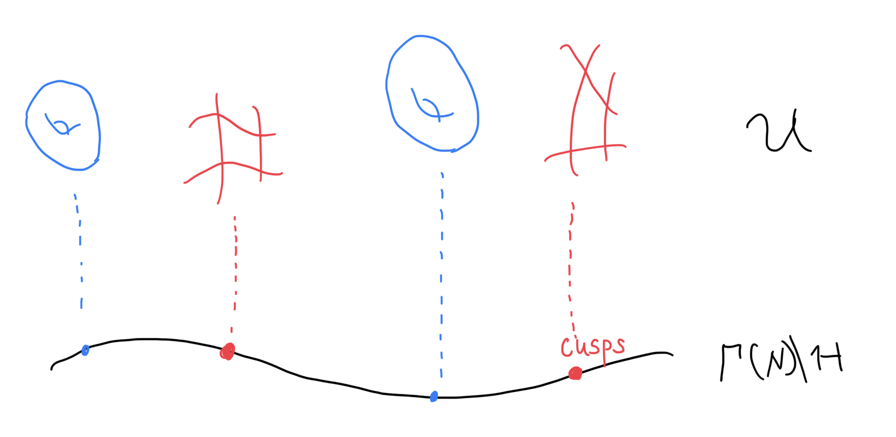
Figure 1. The universal elliptic curve with level $N=4$

We will not do explicit computations on $L_{4,4}$ in this paper. However, it is important to have a glance at the computations in [BKK16] to get a feeling about the singularities on automorphic line bundles. These intuitions inspire our definition of $\mathcal{I}$-good singularities below.

4. Pull-backs of currents

Let $X$ be a complex manifold of pure dimension $n$.

Definition 4.1.

A closed dsh current of bi-dimension $(p,p)$ on $X$ is a current $T$ of bi-dimension $(p,p)$ of the form $T=S_{1}-S_{2}$, where $S_{1}$, $S_{2}$ are closed positive currents of bi-dimension $(p,p)$ on $X$. The set of such currents is denoted by $\hat{Z}_{p}(X)$.

Given $T\in\hat{Z}_{p}(X)$, we will call any expression $T=S_{1}-S_{2}$ as above a decomposition of $T$.

Observe that $\hat{Z}_{p}(X)$ is a real vector space. We endow $\hat{Z}_{p}(X)$ with the weak topology of currents. Thus $\hat{Z}_{p}(X)$ becomes a locally convex topological vector space.

Lemma 4.2.

Let $T\in\hat{Z}_{p}(X)$. Suppose that $T$ puts no mass on a complete pluripolar set $A\subseteq X$, then there is a decomposition $T=S_{1}-S_{2}$ such that $S_{1}$, $S_{2}$ put no masses on $A$.

In the whole paper, a complete pluripolar set on a compact Kähler manifold $X$ means a subset $Z\subseteq X$ such that for any $x\in X$, we can find a neighbourhood $U\subseteq X$ of $x$ and a plurisubharmonic function $\varphi$ on $U$ such that $Z\cap U=\{x\in U:\varphi(x)=-\infty\}$. A complete pluripolar set is sometimes known as a locally complete pluripolar set in the literature.

Proof.

In fact, let $T=S_{1}-S_{2}$ be an arbitrary decomposition, then we consider

(4.1) $$T=\mathds{1}_{X\setminus A}S_{1}-\mathds{1}_{X\setminus A}S_{2}\,.$$

It follows from [BEGZ10, Remark 1.10] that $\mathds{1}_{X\setminus A}S_{i}$ ($i=1,2$) are both closed and positive. Thus, (4.1) is the desired decomposition. ∎

We say a morphism $f:Y\rightarrow X$ between complex analytic spaces has pure relative dimension $d$ if each of the fibers has pure dimension $d$ (or equidimension of dimension $d$). In the literature, this condition is also known as has relative dimension $d$. When $X$ is smooth and $Y$ is Cohen–Macaulay, both $X$ and $Y$ are equidimensional and $\dim Y-\dim X=d$, it follows from miracle flatness that $f$ is flat. But we still prefer to say $f$ is flat of pure relative dimension $d$ in this case, with non-smooth extensions of the results below in mind.

Theorem 4.3 (Dinh–Sibony).

Let $f:Y\rightarrow X$ be a smooth morphism of pure relative dimension $r$ between complex manifolds $Y$ and $X$ of pure dimensions $n+r$ and $n$. Then there is a unique continuous linear map $f^{*}:\widehat{Z}_{a}(X)\rightarrow\widehat{Z}_{a+r}(Y)$ such that the followings hold:

1. When the current is represented by a form, $f^{*}$ is the usual pull-back.

2. When $f$ is an open immersion, $f^{*}$ is the usual restriction.

3. The pull-back is local on $X$: consider $T\in\widehat{Z}_{a}(X)$ and an open subset $U\subseteq X$,

   $$f^{*}(T|_{U})=f^{*}T|_{f^{-1}U}\,.$$

4. In the case of $(1,1)$-currents, this pull-back is the usual one (namely, pulling back the local Kähler potentials).

5. If $T\in\widehat{Z}_{a}(X)$ puts no mass on a complete pluripolar set $A\subseteq X$, then $f^{*}T$ puts no mass on $f^{-1}A$.

6. If $u$ is a locally bounded psh function on $X$, $T\in\widehat{Z}_{a}(X)$, then

   $$f^{*}(\mathrm{dd}^{\mathrm{c}}u\wedge T)=\mathrm{dd}^{\mathrm{c}}f^{*}u\wedge f^{*}T\,.$$

7. If $T\in\widehat{Z}_{a}(X)$ is closed positive, then so is $f^{*}T$.

Here in (6), the product is taken in the sense of Bedford–Taylor. Recall that between complex manifolds, a smooth morphism is the same as a submersive morphism.

We briefly recall the construction of $f^{*}$. Let $\Gamma_{f}\subseteq Y\times X$ be the the graph of $f$. Write $p_{1}:\Gamma_{f}\rightarrow Y$ and $p_{2}:\Gamma_{f}\rightarrow X$ the two natural projections. We wish to define

$$f^{*}T\coloneqq p_{1*}(p_{2}^{*}T\wedge[\Gamma_{f}])\,.$$

Of course, we need to make sense of $p_{2}^{*}T\wedge[\Gamma_{f}]$ as currents. Locally approximate $T$ by smooth forms $T_{i}$, then we define $p_{2}^{*}T\wedge[\Gamma_{f}]$ as the weak limit of $p_{2}^{*}T_{i}\wedge[\Gamma_{f}]$. The existence of the the limit and its independence of the choice of $T_{i}$ are non-trivial facts proved in [DS07].

Proof.

See [DS07] for the proof of the existence and continuity of $f^{*}$ and (1), (2), (3), (4), (7). These are not explicit in [DS07], however, they are all clear from the construction of $f^{*}$. Part (5) follows from Lemma 4.2 and the results proved in [DS07]. In order to prove (6), we may assume that $u$ is smooth, $T$ is closed and positive and $X=\Delta^{n}$. By approximation, we may assume that $T$ is a form. In this case, (6) is clear. ∎

Corollary 4.4.

Let $X,Y,Z$ be complex manifolds of pure dimensions $n$, $n+r$, $n+r+r^{\prime}$. Let $f:Y\rightarrow X$ and $g:Z\rightarrow Y$ be smooth morphisms of pure relative dimensions $r$ and $r^{\prime}$. Then

$$(fg)^{*}=g^{*}f^{*}:\widehat{Z}_{a}(X)\rightarrow\widehat{Z}_{a+r+r^{\prime}}(X)\,.$$

Proof.

Take $T\in\widehat{Z}_{a}(X)$, we want to show that

(4.2) $$(fg)^{*}T=g^{*}f^{*}T\,.$$

As both sides of (4.2) are linear in $T$, we may assume that $T$ is a closed positive current. As both sides of (4.2) are local on $X$, we may assume that $X=\Delta^{n}$. By continuity of pull-back, we may assume that $T$ is represented by a form. In this case, (4.2) is obvious. ∎

We write $\mathcal{A}^{a,a}(X)$ (resp. $\mathcal{A}^{a,a}_{c}(X)$) for the set of smooth real-valued $(a,a)$-forms (resp. smooth real-valued $(a,a)$-forms with compact supports) on $X$.

Corollary 4.5.

Let $X,Y$ be complex manifolds of pure dimension $n$, $m$. Let $f:Y\rightarrow X$ be a smooth morphism of pure relative dimension $m-n$. Consider $T\in\widehat{Z}_{a}(X)$ and $\alpha\in\mathcal{A}^{a+m-n,a+m-n}_{c}(Y)$, then

(4.3) $$\int_{Y}\alpha\wedge f^{*}T=\int_{X}f_{*}\alpha\wedge T\,.$$

Proof.

As $X,Y$ are smooth, $f$ is in fact smooth, $f_{*}\alpha\in\mathcal{A}_{c}^{a,a}(X)$, so the right-hand side of (4.3) makes sense. The problem (4.3) is local on $X$, so we may assume that $X$ is the unit polydisk $\Delta^{n}$. As both sides of (4.3) are linear in $T$, we may further assume that $T$ is closed and positive in $\Delta^{n}$. By approximation, we may further assume that $T$ is represented by a form, in which case, (4.3) is clear. ∎

Corollary 4.6.

Let $X,Y$ be complex manifolds of pure dimension $n$, $m$. Let $f:Y\rightarrow X$ be a smooth morphism of pure relative dimension $m-n$. Consider $T\in\widehat{Z}_{a}(X)$ and $\alpha\in\mathcal{A}^{b,b}_{c}(Y)$. Then

(4.4) $$f_{*}(\alpha\wedge f^{*}T)=f_{*}\alpha\wedge T\,.$$

Proof.

Let $\beta\in\mathcal{A}_{c}^{a-b+m-n,a-b+m-n}(X)$. We need to show that

(4.5) $$\int_{Y}f^{*}\beta\wedge\alpha\wedge f^{*}T=\int_{X}\beta\wedge f_{*}\alpha\wedge T\,.$$

By Corollary 4.5, we can rewrite the left-hand side of (4.5) as

$$\int_{X}f_{*}(f^{*}\beta\wedge\alpha)\wedge T\,.$$

Thus (4.5) follows from the adjunction formula of forms. ∎

Corollary 4.7.

Let $X,Y,X^{\prime}$ be complex manifolds of pure dimension $n$, $m$, $k$. Let $f:Y\rightarrow X$ be a proper map and $g:X^{\prime}\rightarrow X$ be a smooth morphism of pure relative dimension $k-n$. Consider the following Cartesian square

$$\leavevmode\hbox to61.4pt{\vbox to47.96pt{\text{[drawing]}}}\,. {Y^{\prime}} {X^{\prime}} {Y} {X} \scriptstyle{f^{\prime}} \scriptstyle{g^{\prime}} {\square} \scriptstyle{g} \scriptstyle{f} {Y^{\prime}} {X^{\prime}} {Y} {X} \scriptstyle{f^{\prime}} \scriptstyle{g^{\prime}} {\square} \scriptstyle{g} \scriptstyle{f}$$

Then

$$f^{\prime}_{*}g^{\prime*}=g^{*}f_{*}:\widehat{Z}_{a}(Y)\rightarrow\widehat{Z}_{k-n+a}(X^{\prime})\,.$$

Proof.

Take $T\in\widehat{Z}_{a}(Y)$. We need to prove

$$f^{\prime}_{*}g^{\prime*}T=g^{*}f_{*}T\,.$$

We may assume that $T$ is closed positive current. Take $\alpha\in\mathcal{A}_{c}^{k-n+a,k-n+a}(X^{\prime})$, then we are reduced to show

$$\int_{Y^{\prime}}f^{\prime*}\alpha\wedge g^{\prime*}T=\int_{X^{\prime}}\alpha\wedge g^{*}f_{*}T\,.$$

By Corollary 4.5, this is equivalent to

$$\int_{Y}g^{\prime}_{*}f^{\prime*}\alpha\wedge T=\int_{Y}f^{*}g_{*}\alpha\wedge T\,.$$

So we are reduced to show

$$g^{\prime}_{*}f^{\prime*}\alpha=f^{*}g_{*}\alpha\,,$$

which is nothing but the naturality of fiber integration. ∎

5. Relative non-pluripolar products

We fix a complex manifold $X$ of pure dimension $n$. We will extend Vu’s theory [Vu21] of relative non-pluripolar products in this section and prove a few functoriality results.

Definition 5.1.

Suppose $T_{1},\ldots,T_{m}$ are closed positive $(1,1)$-currents on $X$ and $T$ is a closed positive current of bidimension $(p,p)$ on $X$. Then we say that the relative non-pluripolar product $T_{1}\wedge\cdots\wedge T_{m}\cap T$ is well-defined if for each $x\in X$, we can take a local chart $U\cong\Delta^{n}$ containing $x$, on which $T_{i}=\mathrm{dd}^{\mathrm{c}}u_{i}$ for some psh functions $u_{i}$ on $U$, so that if we define

(5.1) $$R_{k}=\mathrm{dd}^{\mathrm{c}}\max\{u_{1},-k\}\wedge\cdots\wedge\mathrm{dd}^{\mathrm{c}}\max\{u_{1},-k\}\wedge T\,,\quad k\in\mathbb{N}$$

using Bedford–Taylor theory, then

(5.2) $$\sup_{k\in\mathbb{N}}\|\mathds{1}_{\{u_{1}>-k,\ldots,u_{m}>-k\}}R_{k}\|_{K}<\infty$$

for each compact subset $K\subseteq U$. Choose a strictly positive smooth real $(1,1)$-form $\omega$ on $X$. The norm $\|\bullet\|_{K}$ is the measure after taking the wedge product with a suitable power of $\omega$. Of course, the condition (5.2) does not depend on the choice of $\omega$.

In this case, we define the relative non-pluripolar product

(5.3) $$T_{1}\wedge\cdots\wedge T_{m}\cap T\coloneqq\lim_{k\to\infty}R_{k}\,,$$

where the limit is a limit of currents.

When $T=[X]$ is the current of integration along $X$, $T_{1}\wedge\cdots\wedge T_{m}\cap T$ is nothing but the non-pluripolar product studied in [BEGZ10]. The general notion is due to [Vu21].

Lemma 5.2 ([Vu21, Lemma 3.1]).

Suppose $T_{1},\ldots,T_{m}$ are closed positive $(1,1)$-currents on $X$ and $T$ is a closed positive current of bidimension $(p,p)$ on $X$. Suppose that $T_{1}\wedge\cdots\wedge T_{m}\cap T$ is well-defined. Then the limit in (5.3) exists. Moreover, for each Borel measurable $(p-m,p-m)$-form $\Phi$ with locally bounded coefficients on $X$ satisfying $\operatorname{Supp}\Phi\Subset X$, we have

$$\int_{X}(\Phi,T_{1}\wedge\cdots\wedge T_{m}\cap T)=\lim_{k\to\infty}\int_{X}(\Phi,R_{k})\,,$$

where $R_{k}$ is defined as in (5.1).

Here the pairing is that between a test form and a current.

Lemma 5.3.

Suppose $T_{1},\ldots,T_{m}$ are closed positive $(1,1)$-currents on $X$ and $T_{1}$, $T_{2}$ are closed positive currents of bidimension $(p,p)$ on $X$. Take $\lambda_{1},\lambda_{2}\geq 0$. Assume that $T_{1}\wedge\cdots\wedge T_{m}\cap T_{1}$ and $T_{1}\wedge\cdots\wedge T_{m}\cap T_{2}$ are both well-defined, then so is $T_{1}\wedge\cdots\wedge T_{m}\cap(\lambda_{1}T_{1}+\lambda_{2}T_{2})$ and

$$T_{1}\wedge\cdots\wedge T_{m}\cap(\lambda_{1}T_{1}+\lambda_{2}T_{2})=\lambda_{1}(T_{1}\wedge\cdots\wedge T_{m}\cap T_{1})+\lambda_{2}(T_{1}\wedge\cdots\wedge T_{m}\cap T_{2})\,.$$

This is obvious from the definition.

Definition 5.4.

Suppose $T_{1},\ldots,T_{m}$ are closed positive $(1,1)$-currents on $X$ and $T\in\hat{Z}_{p}(X)$. We say the relative non-pluripolar product $T_{1}\wedge\cdots\wedge T_{m}\cap T$ is well-defined if there is a decomposition $T=S_{1}-S_{2}$ such that $T_{1}\wedge\cdots\wedge T_{m}\cap S_{i}$ ($i=1,2$) are both well-defined.

In this case, we define

$$T_{1}\wedge\cdots\wedge T_{m}\cap T\coloneqq T_{1}\wedge\cdots\wedge T_{m}\cap S_{1}-T_{1}\wedge\cdots\wedge T_{m}\cap S_{2}\,.$$

Observe that the product $T_{1}\wedge\cdots\wedge T_{m}\cap T$ is symmetric in $T_{i}$.

Lemma 5.5.

Suppose $T_{1},\ldots,T_{m}$ are closed positive $(1,1)$-currents on $X$ and $T\in\hat{Z}_{p}(X)$. Assume that $T_{1}\wedge\cdots\wedge T_{m}\cap T$ is well-defined, then $T_{1}\wedge\cdots\wedge T_{m}\cap T$ does not depend on the choice of the decomposition $T=S_{1}-S_{2}$.

Proof.

This follows immediately from Lemma 5.3. ∎

Proposition 5.6.

Suppose $T_{1},\ldots,T_{m}$ are closed positive $(1,1)$-currents on $X$ and $T_{1},T_{2}\in\hat{Z}_{p}(X)$. Take $\lambda_{1},\lambda_{2}\in\mathbb{R}$. Assume that $T_{1}\wedge\cdots\wedge T_{m}\cap T_{1}$ and $T_{1}\wedge\cdots\wedge T_{m}\cap T_{2}$ are both well-defined, then so is $T_{1}\wedge\cdots\wedge T_{m}\cap(\lambda_{1}T_{1}+\lambda_{2}T_{2})$ and

(5.4) $$T_{1}\wedge\cdots\wedge T_{m}\cap(\lambda_{1}T_{1}+\lambda_{2}T_{2})=\lambda_{1}(T_{1}\wedge\cdots\wedge T_{m}\cap T_{1})+\lambda_{2}(T_{1}\wedge\cdots\wedge T_{m}\cap T_{2})\,.$$

Proof.

We may assume that $\lambda_{1},\lambda_{2}\geq 0$.

By definition, we can find closed positive currents $S_{1}^{1}$, $S_{1}^{2}$, $S_{2}^{1}$, $S_{2}^{2}$ of bidimension $(p,p)$ such that $T_{1}=S_{1}^{1}-S_{1}^{2}$, $T_{2}=S_{2}^{1}-S_{2}^{2}$ and $T_{1}\wedge\cdots\wedge T_{m}\cap S_{i}^{j}$ ($i=1,2$, $j=1,2$) are all well-defined. Then $T_{1}\wedge\cdots\wedge T_{m}\cap(\lambda_{1}S_{1}^{j}+\lambda_{2}S_{2}^{j})$ ($j=1,2$) are both well-defined. Hence so is $T_{1}\wedge\cdots\wedge T_{m}\cap(\lambda_{1}T_{1}+\lambda_{2}T_{2})$ and (5.4) follows. ∎

On the other hand, the product $T_{1}\wedge\cdots\wedge T_{m}\cap T$ is not additive in $T_{i}$ in general.

Proposition 5.7.

Suppose $T_{1},\ldots,T_{m}$ and $T_{1}^{\prime}$ are closed positive $(1,1)$-currents on $X$ and $T\in\hat{Z}_{p}(X)$. Assume that $T_{1}\wedge T_{2}\wedge\cdots\wedge T_{m}\cap T$ and $T_{1}^{\prime}\wedge T_{2}\wedge\cdots\wedge T_{m}\cap T$ are both well-defined, then so is $(T_{1}+T_{1}^{\prime})\wedge T_{2}\wedge\cdots\wedge T_{m}\cap T$.

Furthermore, if $T$ puts no mass on the polar loci of $T_{1}$ and $T_{1}^{\prime}$, then

$$(T_{1}+T_{1}^{\prime})\wedge T_{2}\wedge\cdots\wedge T_{m}\cap T=T_{1}\wedge T_{2}\wedge\cdots\wedge T_{m}\cap T+T_{1}^{\prime}\wedge T_{2}\wedge\cdots\wedge T_{m}\cap T\,.$$

Recall that the polar locus of a closed positive $(1,1)$-current $T$ is locally defined as $\{\varphi=-\infty\}$ when the current $T$ is written as $\mathrm{dd}^{\mathrm{c}}\varphi$ locally.

Proof.

This follows from [Vu21, Proposition 3.5(iv)] and Lemma 4.2. ∎

Proposition 5.8.

Suppose $T_{1},\ldots,T_{m}$ are closed positive $(1,1)$-currents on $X$ and $T\in\hat{Z}_{p}(X)$. Assume that $T_{1}\wedge\cdots\wedge T_{m}\cap T$ is well-defined, then $T_{1}\wedge\cdots\wedge T_{m}\cap T\in\hat{Z}_{a-m}(X)$.

Proof.

This follows immediately from [Vu21, Theorem 3.7, Lemma 3.2(ii)]. ∎

Proposition 5.9.

Suppose $T_{1},\ldots,T_{m}$ are closed positive $(1,1)$-currents on $X$ and $T\in\hat{Z}_{p}(X)$ and $T_{1}\wedge\cdots\wedge T_{m}\cap T$ is well-defined. Assume that $T$ puts no mass on a complete pluripolar set $A\subseteq X$, then so is $T_{1}\wedge\cdots\wedge T_{m}\cap T$.

Proof.

This follows from Lemma 4.2. ∎

Proposition 5.10.

Suppose $T_{1},\ldots,T_{m}$ are closed positive $(1,1)$-currents on $X$ and $T\in\hat{Z}_{p}(X)$. Fix an integer $b$ with $1\leq b\leq m$. Assume that $R=T_{b+1}\wedge\cdots\wedge T_{m}\cap T$ is well-defined and $T_{1}\wedge\cdots\wedge T_{b}\cap R$ is well-defined. Then $T_{1}\wedge\cdots\wedge T_{m}\cap T$ is well-defined and

$$T_{1}\wedge\cdots\wedge T_{m}\cap T=T_{1}\wedge\cdots\wedge T_{b}\cap R=T_{1}\wedge\cdots\wedge T_{b}\cap(T_{b+1}\wedge\cdots\wedge T_{m}\cap T)\,.$$

Proof.

This follows from [Vu21, Proposition 3.5(vi)]. ∎

Proposition 5.11.

Suppose $T_{1},\ldots,T_{m}$ are closed positive $(1,1)$-currents on $X$ and $T\in\hat{Z}_{p}(X)$. Assume that $X$ is a compact Kähler manifold, then $T_{1}\wedge\cdots\wedge T_{m}\cap T$ is well-defined.

Proof.

This follows from [Vu21, Lemma 3.4]. ∎

Proposition 5.12.

Let $f:Y\rightarrow X$ be a proper morphism of complex manifolds. Assume that the $f^{*}T_{i}$’s are defined in the sense that $f$ does not map any of the connected components of $Y$ into the polar loci of any $T_{i}$. Suppose $T_{1},\ldots,T_{m}$ are closed positive $(1,1)$-currents on $X$ and $T\in\hat{Z}_{p}(Y)$. Suppose that $T_{1}\wedge\cdots\wedge T_{m}\cap f_{*}T$ and $f^{*}T_{1}\wedge\cdots\wedge f^{*}T_{m}\cap T$ are both well-defined. In this case,

(5.5) $$f_{*}(f^{*}T_{1}\wedge\cdots\wedge f^{*}T_{m}\cap T)=T_{1}\wedge\cdots\wedge T_{m}\cap f_{*}T\,.$$

Proof.

We may assume that $T$ is a closed positive current.

The problem is local on $X$, we may assume that $X\cong\Delta^{n}$ and $T_{i}=\mathrm{dd}^{\mathrm{c}}u_{i}$ for some psh functions $u_{i}$ on $\Delta^{n}$.

Observe that for any $k\in\mathbb{Z}$,

$$\mathrm{dd}^{\mathrm{c}}\max\{u_{1},-k\}\wedge\cdots\wedge\mathrm{dd}^{\mathrm{c}}\{u_{1},-k\}\wedge f_{*}T=f_{*}\left(\mathrm{dd}^{\mathrm{c}}\max\{f^{*}u_{1},-k\}\wedge\cdots\wedge\mathrm{dd}^{\mathrm{c}}\{f^{*}u_{1},-k\}\wedge T\right)\,.$$

Let $k\to\infty$, (5.5) follows from the continuity of $f_{*}$. ∎

Proposition 5.13.

Suppose $T_{1},\ldots,T_{m}$ are closed positive $(1,1)$-currents on $X$ with locally bounded potentials and $T\in\hat{Z}_{p}(X)$. Then $T_{1}\wedge\cdots\wedge T_{m}\cap T$ is well-defined and

$$T_{1}\wedge\cdots\wedge T_{m}\cap T=T_{1}\wedge\cdots\wedge T_{m}\wedge T\,.$$

Here on the right-hand side, we make use of Bedford–Taylor theory.

Proof.

This follows from [Vu21, Proposition3.6]. ∎

Proposition 5.14.

Let $Y$ be a complex manifold of pure dimension $m$. Let $f:Y\rightarrow X$ be a smooth morphism of pure relative dimension $m-n$. Suppose $T_{1},\ldots,T_{m}$ are closed positive $(1,1)$-currents on $X$ and $T\in\hat{Z}_{p}(X)$. Assume that $f^{*}T_{1}\wedge\cdots\wedge f^{*}T_{m}\cap f^{*}T$ and $T_{1}\wedge\cdots\wedge T_{m}\cap T$ are both well-defined, then

(5.6) $$f^{*}T_{1}\wedge\cdots\wedge f^{*}T_{m}\cap f^{*}T=f^{*}\left(T_{1}\wedge\cdots\wedge T_{m}\cap T\right)$$

Proof.

Step 1. We first show that (5.6) holds if $T_{1},\ldots,T_{m}$ all have locally bounded potentials. In this case, by Proposition 5.13, (5.6) is equivalent to

(5.7) $$f^{*}T_{1}\wedge\cdots\wedge f^{*}T_{m}\wedge f^{*}T=f^{*}\left(T_{1}\wedge\cdots\wedge T_{m}\wedge T\right)\,.$$

By induction, we reduce immediately to the case $m=1$. The problem is local on $X$, so we are reduced to Theorem 4.3(6).

Step 2. We handle the general case. We may assume that $T$ is a closed positive current.

The problem is local on $X$, we may assume that $X\cong\Delta^{n}$ and $T_{i}=\mathrm{dd}^{\mathrm{c}}u_{i}$ for some psh functions $u_{i}$ on $\Delta^{n}$. In this case,

$$f^{*}T_{1}\wedge\cdots\wedge f^{*}T_{m}\cap f^{*}T=\lim_{k\to\infty}\mathrm{dd}^{\mathrm{c}}f^{*}\max\{u_{1},-k\}\wedge\cdots\wedge\mathrm{dd}^{\mathrm{c}}f^{*}\{u_{1},-k\}\wedge f^{*}T\,.$$

By Step 1,

$$f^{*}T_{1}\wedge\cdots\wedge f^{*}T_{m}\cap f^{*}T=\lim_{k\to\infty}f^{*}(\mathrm{dd}^{\mathrm{c}}\max\{u_{1},-k\}\wedge\cdots\wedge\mathrm{dd}^{\mathrm{c}}\{u_{1},-k\}\wedge T)\,.$$

Then (5.6) follows from the continuity of $f^{*}$ Theorem 4.3. ∎

6. Segre currents and Chern currents

In this section, let $X$ be a compact Kähler manifold of pure dimension $n$. We will define Segre currents and Chern currents following the approach of [Ful98, Chapter 3].

6.1. First Chern class

Definition 6.1.

For any $T\in\widehat{Z}_{a}(X)$ and any $\hat{L}=(L,h_{L})\in\widehat{\mathrm{Pic}}(X)$, we define

(6.1) $$c_{1}(\hat{L})\cap T=\mathrm{dd}^{\mathrm{c}}h_{L}\cap T\in\widehat{Z}_{a-1}(X)\,.$$

Note that $c_{1}(\hat{L})\cap T\in\widehat{Z}_{a-1}(X)$ as a consequence of Proposition 5.8.

We remind the readers that $c_{1}(\hat{L})$ is defined as an operator on the space of currents instead of a class in certain Chow groups. This is a key difference with the usual intersection theory and is the main innovation of this paper. This point of view will be helpful when we consider the intersection theory on the Riemann–Zariski spaces as well.

We can translate the results in Section 5 in terms of $c_{1}$. Firstly we have the commutativity of $c_{1}$.

Lemma 6.2.

Let $T\in\hat{Z}_{a}(X)$, $\hat{L}_{i}\in\widehat{\mathrm{Pic}}(X)$ ($i=1,2$). Then

$$c_{1}(\hat{L}_{1})\cap\left(c_{1}(\hat{L}_{2})\cap T\right)=c_{1}(\hat{L}_{2})\cap\left(c_{1}(\hat{L}_{1})\cap T\right)\,.$$

Proof.

This follows from Proposition 5.10. ∎

The functorality results in Section 5 can be put in the familiar form now.

Lemma 6.3.

Assume that $Y$ is a compact Kähler manifold of pure dimension $m$. Let $\hat{L}\in\widehat{\mathrm{Pic}}(X)$.

1. Let $f:Y\rightarrow X$ be a proper morphism, $T\in\widehat{Z}_{a}(Y)$, then if the metric on $f^{*}\hat{L}$ is not identically $\infty$ on each connected component of $Y$,

   $$f_{*}(c_{1}(f^{*}\hat{L})\cap T)=c_{1}(\hat{L})\cap f_{*}T\,.$$

2. Let $f:Y\rightarrow X$ be a smooth morphism of pure relative dimension $m-n$. Let $\hat{L}\in\widehat{\mathrm{Pic}}(X)$, $T\in\widehat{Z}_{a}(X)$, then

   $$f^{*}(c_{1}(\hat{L})\cap T)=c_{1}(f^{*}\hat{L})\cap f^{*}T\,.$$

Proof.

(1) follows from Proposition 5.12 and (2) follows from Proposition 5.14. ∎

Proposition 6.4.

Assume that $\hat{L}=(L,h_{L})\in\widehat{\mathrm{Pic}}(X)$ and $T\in\widehat{Z}_{a}(X)$. If $h_{L}$ is bounded, then

$$c_{1}(\hat{L})\cap T=\mathrm{dd}^{\mathrm{c}}h_{L}\wedge T\,.$$

Proof.

This follows from Proposition 5.13. ∎

In general, $c_{1}(\hat{L})\cap T$ is not linear in $\hat{L}$, we need a technical assumption:

Definition 6.5.

We say $\hat{E}\in\widehat{\mathrm{Vect}}(X)$ or $\widehat{\mathrm{Vect}}^{F}(X)$ is transversal to $T\in\widehat{Z}_{a}(X)$ (or $T$ is transversal to $E$) if $p^{*}T$ (with $p:\mathbb{P}E^{\vee}\rightarrow X$ being the natural map) does not have mass on the polar locus of $\hat{\mathcal{O}}(1)$.

In the special case $\hat{L}\in\widehat{\mathrm{Pic}}(X)$, $\hat{L}$ is transversal to $T$ if and only if $T$ does not have mass on the polar locus of $\hat{L}$. The following simple observation will be quite useful:

Lemma 6.6.

Let $T\in\widehat{Z}_{a}(X)$ and $A$ be a complete pluripolar subset of $X$. Let $p:Y\rightarrow X$ be a smooth morphism of pure relative dimension $b$ from a compact Kähler manifold $Y$ of pure dimension $n+b$. Then $p^{*}T$ does not have mass on $p^{-1}A$ if and only if $T$ does not have mass on $A$.

In particular, if $\hat{E}\in\widehat{\mathrm{Vect}}(X)$ is transversal to $T$ if and only if $T$ does not have mass on the polar locus of $\hat{E}$.

Proof.

This follows from Corollary 4.6 and Theorem 4.3 (5). ∎

Lemma 6.7.

Let $\hat{E}\in\widehat{\mathrm{Vect}}(X)$ or $\widehat{\mathrm{Vect}}^{F}(X)$, $f:Y\rightarrow X$ be a smooth morphism of pure relative dimension $d$ from a compact Kähler manifold $Y$ of pure dimension $n+d$. Assume that $T\in\widehat{Z}_{a}(X)$ is transversal to $\hat{E}$, then $f^{*}T$ is transversal to $f^{*}\hat{E}$.

Proof.

Consider the Cartesian square

We need to show that $p^{\prime*}f^{*}T=f^{\prime*}p^{*}T$ does not have mass on the polar locus of $\hat{\mathcal{O}}_{\mathbb{P}(f^{*}\hat{E})^{\vee}}(1)$, which is equal to the inverse image of the polar locus of $\hat{\mathcal{O}}_{\mathbb{P}E^{\vee}}(1)$. By Lemma 6.6, it suffices to show that $p^{*}T$ does not have mass on the polar locus of $\hat{\mathcal{O}}_{\mathbb{P}E^{\vee}}(1)$, which holds by our assumption. ∎

Lemma 6.8.

Let $T\in\hat{Z}_{a}(X)$, $\hat{L}_{i}\in\widehat{\mathrm{Pic}}(X)$. Assume that $T$ is transversal to both $\hat{L}_{1}$ and $\hat{L}_{2}$. Then

$$c_{1}(\hat{L}_{1}\otimes\hat{L}_{2})\cap T=c_{1}(\hat{L}_{1})\cap T+c_{1}(\hat{L}_{2})\cap T\,.$$

Proof.

This follows from Proposition 5.7. ∎

Proposition 6.9.

Assume that $\hat{L}\in\widehat{\mathrm{Pic}}(X)$ and $T\in\widehat{Z}_{a}(X)$. Let $A\subseteq X$ be a pluripolar set such that $T$ does not have mass on $A$. Then $c_{1}(\hat{L})\cap T$ also does not have mass on $A$.

Proof.

This follows from [Vu21, Proposition 3.9(iii)]. ∎

Corollary 6.10.

Let $T\in\hat{Z}_{a}(X)$, $\hat{L}_{i}\in\widehat{\mathrm{Pic}}(X)$ ($i=1,2$). Suppose that $T$ is transversal to both $\hat{L}_{1}$ and $\hat{L}_{2}$, then $c_{1}(\hat{L}_{2})\cap T$ is transversal to $\hat{L}_{1}$.

6.2. Segre classes

Consider $\hat{E}=(E,h_{E})\in\widehat{\mathrm{Vect}}(X)$ of rank $r+1$. Let $p=p_{E}:\mathbb{P}E^{\vee}\rightarrow X$ be the projective bundle associated with $E^{\vee}$. We defined $\hat{\mathcal{O}}(1)\in\widehat{\mathrm{Pic}}(\mathbb{P}E^{\vee})$ in Section 3.3. Every result proved in this section works equally well for $\hat{E}\in\widehat{\mathrm{Vect}}^{F}(X)$.

Definition 6.11.

Consider $\hat{E}=(E,h_{E})\in\widehat{\mathrm{Vect}}(X)$ or $\widehat{\mathrm{Vect}}^{F}(X)$ of rank $r+1$. Define the $i$-th Serge class $s_{i}(\hat{E})\cap:\widehat{Z}_{a}(X)\rightarrow\widehat{Z}_{a-i}(X)$ as follows: let $T\in\widehat{Z}_{a}(X)$, then we set

(6.2) $$s_{i}(\hat{E})\cap T=(-1)^{i}p_{*}\left(c_{1}(\widehat{\mathcal{O}}(1))^{r+i}\cap p^{*}T\right)\,.$$

Here $c_{1}(\widehat{\mathcal{O}}(1))^{r+i}\cap$ is short for iterated application of $c_{1}(\widehat{\mathcal{O}}(1))\cap\bullet$ for $(r+i)$ times.

We show that the Segre classes satisfy the usual functoriality.

Proposition 6.12.

Let $Y$ be a compact Kähler manifold of pure dimension $m$.

1. Let $f:Y\rightarrow X$ be a proper morphism, $\hat{E}\in\widehat{\mathrm{Vect}}(X)$ or $\widehat{\mathrm{Vect}}^{F}(X)$, $T\in\widehat{Z}_{a}(Y)$. Assume that the metric on $f^{*}\hat{E}$ is not identically $\infty$ on each connected component of $Y$. Then for all $i$,

   $$f_{*}(s_{i}(f^{*}\hat{E})\cap T)=s_{i}(\hat{E})\cap f_{*}T$$

2. Let $f:Y\rightarrow X$ be a smooth morphism of pure relative dimension $m-n$, $\hat{E}\in\widehat{\mathrm{Vect}}(X)$ or $\widehat{\mathrm{Vect}}^{F}(X)$, $T\in\widehat{Z}_{a}(X)$. Then for all $i$,

   $$f^{*}(s_{i}(\hat{E})\cap T)=s_{i}(f^{*}\hat{E})\cap f^{*}T\,.$$

Proof.

Let $\rank E=r+1$.

In both cases, consider the Cartesian square

It is well-known that $f^{\prime*}\mathcal{O}_{\mathbb{P}E^{\vee}}(1)=\mathcal{O}_{\mathbb{P}(f^{*}E)^{\vee}}(1)$. A direct verification shows that it preserves the metric as well. Namely,

(6.3) $$f^{\prime*}\hat{\mathcal{O}}_{\mathbb{P}E^{\vee}}(1)=\hat{\mathcal{O}}_{\mathbb{P}(f^{*}E^{\vee})}(1)\,.$$

(1) Consider $T\in\widehat{Z}_{a}(Y)$, then

$$(-1)^{i}f_{*}(s_{i}(f^{*}\hat{E})\cap T)= f_{*}p^{\prime}_{*}\left(c_{1}(\hat{\mathcal{O}}_{\mathbb{P}(f^{*}E^{\vee})}(1))^{r+i}\cap p^{\prime*}T\right)$$

$$= (-1)^{i}p_{*}f^{\prime}_{*}\left(c_{1}(f^{\prime*}\hat{\mathcal{O}}_{\mathbb{P}E^{\vee}}(1))^{r+i}\cap p^{\prime*}T\right) \eqref{eq:hOpreserved}$$

$$= (-1)^{i}p_{*}\left(c_{1}(\hat{\mathcal{O}}_{\mathbb{P}E^{\vee}}(1))^{r+i}\cap f^{\prime}_{*}p^{\prime*}T\right)$$ Lemma 6.3

$$= (-1)^{i}p_{*}\left(c_{1}(\hat{\mathcal{O}}_{\mathbb{P}E^{\vee}}(1))^{r+i}\cap p^{*}f_{*}T\right)$$ Corollary 4.7

$$= (-1)^{i}s_{i}(\hat{E})\cap f_{*}T \,.$$

(2) Consider $T\in\widehat{Z}_{a}(X)$, then

$$(-1)^{i}s_{i}(f^{*}\hat{E})\cap f^{*}T= p^{\prime}_{*}\left(c_{1}(\hat{\mathcal{O}}_{\mathbb{P}(f^{*}E^{\vee})}(1))^{r+i}\cap p^{\prime*}f^{*}T\right)$$

$$= p^{\prime}_{*}\left(f^{\prime*}c_{1}(\hat{\mathcal{O}}_{\mathbb{P}E^{\vee}}(1))^{r+i}\cap f^{\prime*}p^{*}T\right)$$

$$= p^{\prime}_{*}f^{\prime*}\left(c_{1}(\hat{\mathcal{O}}_{\mathbb{P}E^{\vee}}(1))^{r+i}\cap p^{*}T\right)$$ Lemma 6.3

$$= f^{*}p_{*}\left(c_{1}(\hat{\mathcal{O}}_{\mathbb{P}E^{\vee}}(1))^{r+i}\cap p^{*}T\right)$$ Corollary 4.7

$$= (-1)^{i}f^{*}(s_{i}(\hat{E})\cap T) \,.$$

∎

Proposition 6.13.

Consider $\hat{E}\in\widehat{\mathrm{Vect}}(X)$ or $\widehat{\mathrm{Vect}}^{F}(X)$ and $T\in\widehat{Z}_{a}(X)$. Suppose that $T$ does not have mass on a complete pluripolar set $A\subseteq X$, then so is $s_{i}(\hat{E})\cap T$.

Proof.

First observe that $p^{*}T$ does not have mass on $A$ by Theorem 4.3(5). By an iterated application of Proposition 6.9, $c_{1}(\widehat{\mathcal{O}}(1))^{r+i}\cap p^{*}T$ does not have mass on $p^{-1}A$. By Corollary 4.6, $s_{i}(\hat{E})\cap T$ does not have mass on $A$. ∎

So our intersection theory is indeed a non-pluripolar theory. The transversality is preserved by the Segre classes.

Corollary 6.14.

Consider $\hat{E},\hat{F}\in\widehat{\mathrm{Vect}}(X)$ or $\widehat{\mathrm{Vect}}^{F}(X)$ and $T\in\widehat{Z}_{a}(X)$. Suppose that $T$ is transversal to both $\hat{E}$ and $\hat{F}$. Then $s_{i}(\hat{E})\cap T$ is transversal to $\hat{F}$.

Proof.

Let $q:\mathbb{P}F^{\vee}\rightarrow X$ be the natural projection. By definition, we need to show that $\hat{\mathcal{O}}_{\mathbb{P}F^{\vee}}(1)$ is transversal to $q^{*}(s_{i}(\hat{E})\cap T)$. By Proposition 6.12, the latter is equal to $s_{i}(q^{*}\hat{E})\cap q^{*}T$. By Lemma 6.7, $q^{*}T$ is transversal to $q^{*}\hat{E}$ and $q^{*}T$ is transversal to $\hat{\mathcal{O}}_{\mathbb{P}F^{\vee}}(1)$ by assumption. So we are reduced to the case where $F$ is a line bundle. In this case, it suffices to apply Proposition 6.13. ∎

Proposition 6.15.

Consider $\hat{E}\in\widehat{\mathrm{Vect}}(X)$ or $\widehat{\mathrm{Vect}}^{F}(X)$ and $T\in\widehat{Z}_{a}(X)$. Then $s_{i}(\hat{E})\cap T=0$ if $i<0$.

Proof.

The problem is local on $X$, so we may assume that $E$ is the trivial vector bundle of rank $r+1$ and $X=\Delta^{n}$. Take $\eta\in\mathcal{A}_{c}^{a-i,a-i}(X)$, then

$$\begin{split}\int_{X}\eta\wedge(s_{i}(\hat{E})\cap T)=&\int_{\mathbb{P}E^{\vee}}p^{*}\eta\wedge\left(c_{1}(\hat{\mathcal{O}}(1))^{r+i}\cap p^{*}T\right)\,.\end{split}$$

Fix a smooth form $\Theta\in c_{1}(\mathcal{O}(1))$ and identify the metric on $\hat{\mathcal{O}}(1)$ with $\Phi\in\mathrm{PSH}(\mathbb{P}E^{\vee},\Theta)$. By [Vu21, Lemma 3.2],

$$\int_{\mathbb{P}E^{\vee}}p^{*}\eta\wedge\left(c_{1}(\hat{\mathcal{O}}(1))^{r+i}\cap p^{*}T\right)=\lim_{k\to\infty}\int_{\mathbb{P}E^{\vee}}p^{*}\eta\wedge\mathds{1}_{\{\Phi>-k\}}\Theta_{\max\{\Phi,-k\}}^{r+i}\wedge p^{*}T\,.$$

Assume that $i<0$. It suffices to prove more generally that for any bounded $\Psi\in\mathrm{PSH}(\mathbb{P}E^{\vee},\Theta)$,

(6.4) $$p^{*}\eta\wedge\Theta_{\Psi}^{r+i}\wedge p^{*}T=0\,.$$

By regularization and possibly passing to an open subset of $\mathbb{P}E^{\vee}$, we may assume that $\Psi$ is smooth. Then a simple degree counting proves (6.4). ∎

Proposition 6.16.

Let $\hat{E},\hat{F}\in\widehat{\mathrm{Vect}}(X)$ or $\widehat{\mathrm{Vect}}^{F}(X)$, $T\in\widehat{Z}_{a}(X)$. For any $b,c$ we have

(6.5) $$s_{c}(\hat{E})\cap s_{b}(\hat{F})\cap T=s_{b}(\hat{F})\cap s_{c}(\hat{E})\cap T\,.$$

Remark 6.17.

This result is of course what one should expect from classical intersection theory. However, we want to emphasize that it is by no means trivial, as one would imagine at a first glance. A priori, there are not many evidences indicating that non-pluripolar intersection theory is better than the other Hermitian intersection theory. This result marks the big advantage of our theory. In fact, the corresponding results fail in the theory of Chern currents of Lärkäng–Raufi–Ruppenthal–Sera [LRRS18].

Proof.

Write $\rank E=r+1$ and $\rank F=s+1$.

Consider the Cartesian square

$$\leavevmode\hbox to78.08pt{\vbox to49.52pt{\text{[drawing]}}}\,. {Y} {\mathbb{P}F^{\vee}} {\mathbb{P}E^{\vee}} {X} \scriptstyle{p^{\prime}} \scriptstyle{q^{\prime}} {\square} \scriptstyle{q} \scriptstyle{p} {Y} {\mathbb{P}F^{\vee}} {\mathbb{P}E^{\vee}} {X} \scriptstyle{p^{\prime}} \scriptstyle{q^{\prime}} {\square} \scriptstyle{q} \scriptstyle{p}$$

We compute the left-hand side of (6.5):

$$\begin{aligned} &(-1)^{c+b}s_{c}(\hat{E})\cap s_{b}(\hat{F})\cap T&\\ =&(-1)^{c}s_{c}(\hat{E})\cap q_{*}\left(c_{1}(\hat{\mathcal{O}}_{\mathbb{P}F^{\vee}}(1))^{b+s}\cap q^{*}T\right)&\\ =&(-1)^{c}q_{*}\left(s_{c}(q^{*}\hat{E})\cap c_{1}(\hat{\mathcal{O}}_{\mathbb{P}F^{\vee}}(1))^{b+s}\cap q^{*}T\right)&\lx@cref{creftype~refnum}{prop:projectionform}\\ =&q_{*}p^{\prime}_{*}\left(c_{1}(q^{\prime*}\hat{\mathcal{O}}_{\mathbb{P}E^{\vee}}(1))^{c+r}\cap p^{\prime*}\left(c_{1}(\hat{\mathcal{O}}_{\mathbb{P}F^{\vee}}(1))^{b+s}\cap q^{*}T\right)\right)&\\ =&q_{*}p^{\prime}_{*}\left(q^{\prime*}c_{1}(\hat{\mathcal{O}}_{\mathbb{P}E^{\vee}}(1))^{c+r}\cap p^{\prime*}c_{1}(\hat{\mathcal{O}}_{\mathbb{P}F^{\vee}}(1))^{b+s}\cap p^{\prime*}q^{*}T\right)&\lx@cref{creftype~refnum}{prop:firstChernformpush}\\ =&q_{*}p^{\prime}_{*}\left(p^{\prime*}c_{1}(\hat{\mathcal{O}}_{\mathbb{P}F^{\vee}}(1))^{b+s}\cap q^{\prime*}c_{1}(\hat{\mathcal{O}}_{\mathbb{P}E^{\vee}}(1))^{c+r}\cap p^{\prime*}q^{*}T\right)&\lx@cref{creftype~refnum}{prop:c1comm}\end{aligned}\,.$$

Now run the same computation again for the right-hand side of (6.5), we get the same expression. ∎

From the proof, we get

Corollary 6.18.

Let $\hat{E}_{i}\in\widehat{\mathrm{Vect}}(X)$ or $\widehat{\mathrm{Vect}}^{F}(X)$ ($i=1,\ldots,m$), $T\in\widehat{Z}_{a}(X)$. Write $\rank E_{i}=r_{i}+1$. Let $Y=\mathbb{P}E_{1}^{\vee}\times_{X}\cdots\times_{X}\mathbb{P}E_{m}^{\vee}$. Let $\pi:Y\rightarrow X$, $\pi_{i}:Y\rightarrow\mathbb{P}E_{i}^{\vee}$ be the natural projections. Then for any integers $b_{i}$,

$$\begin{split}(-1)^{b_{1}+\cdots+b_{m}}s_{b_{1}}(\widehat{E}_{1})\cap\cdots\cap s_{b_{m}}(\widehat{E}_{m})\cap T=\pi_{*}\left(\pi_{1}^{*}c_{1}(\hat{\mathcal{O}}_{\mathbb{P}E_{1}^{\vee}}(1))^{a_{1}+r_{1}}\cap\cdots\right.\\ \left.\cap\pi_{m}^{*}c_{m}(\hat{\mathcal{O}}_{\mathbb{P}E_{m}^{\vee}}(1))^{a_{m}+r_{m}}\cap\pi^{*}T\right)\,.\end{split}$$

Proposition 6.19.

Let $\hat{E}=(E,h_{E})\in\widehat{\mathrm{Vect}}(X)$ or $\widehat{\mathrm{Vect}}^{F}(X)$, $T\in\widehat{Z}_{a}(X)$. Assume that $h_{E}$ is locally bounded on an open set $U\subseteq X$, then

(6.6) $$(s_{m}(\hat{E})\cap T)|_{U}=s_{m}(\hat{E}|_{U})\wedge T|_{U}\,.$$

Here $s_{m}(\hat{E}|_{U})$ is defined using the same formula as $s_{m}(\hat{E})$:

$$s_{m}(\hat{E}|_{U})\wedge T|_{U}\coloneqq(-1)^{m}p_{*}\left(c_{1}(\hat{\mathcal{O}}(1))^{r+i}\wedge p^{*}T|_{U}\right)\,,$$

where $\rank E=r+1$ and $p:\mathbb{P}E|_{U}^{\vee}\rightarrow U$ is the natural projection.

Proof.

This follows from Proposition 5.13. ∎

It is easy to reproduce the well-known formulae about Segre classes in our setting, for example:

Proposition 6.20.

Let $\hat{E}=(E,h_{E})\in\widehat{\mathrm{Vect}}(X)$ or $\widehat{\mathrm{Vect}}^{F}(X)$, $\hat{L}\in\widehat{\mathrm{Pic}}(X)$ and $T\in\widehat{Z}_{a}(X)$. Assume that $T$ is transversal to $\hat{E}$ and $\hat{L}$. Write $\rank E=r+1$, then

(6.7) $$s_{a}(\hat{E}\otimes\hat{L})\cap T=\sum_{j=0}^{a}\binom{a+r}{j+r}(-1)^{a+j}s_{j}(\hat{E})\cap c_{1}(\hat{L})^{a-j}\cap T\,.$$

Proof.

Let $p:\mathbb{P}E^{\vee}\rightarrow X$ be the natural projection. We compute

$$s_{a}(\hat{E}\otimes\hat{L})\cap T$$

$$= p_{*}\left(c_{1}(\hat{\mathcal{O}}_{\mathbb{P}(E\otimes L)^{\vee}}(1))^{a+r}\cap p^{*}T\right)$$

$$= (-1)^{a}\sum_{j=0}^{a+r}\binom{a+r}{j}p_{*}\left(c_{1}(\hat{\mathcal{O}}_{\mathbb{P}E^{\vee}}(1))^{j}\cap c_{1}(p^{*}\hat{L})^{a+r-j}\cap p^{*}T\right)$$ Lemma 6.8

$$= (-1)^{a}\sum_{j=0}^{a+r}\binom{a+r}{j}(-1)^{j-r}s_{j-r}(\hat{E})\cap p_{*}\left(c_{1}(p^{*}\hat{L})^{a+r-j}\cap p^{*}T\right)$$

$$= \sum_{j=0}^{a+r}\binom{a+r}{j}(-1)^{j-r+a}s_{j-r}(\hat{E})\cap c_{1}(\hat{L})^{a+r-j}\cap T$$ Corollary 4.6

$$= \sum_{j=0}^{a}\binom{a+r}{j+r}(-1)^{a+j}s_{j}(\hat{E})\cap c_{1}(\hat{L})^{a-j}\cap T \lx@cref{creftype~refnum}{prop:negsegvan}\,.$$

∎

6.3. Chern Polynomials

Definition 6.21.

Let $\hat{E}_{1},\ldots,\hat{E}_{b}\in\widehat{\mathrm{Vect}}(X)$ or $\widehat{\mathrm{Vect}}^{F}(X)$. Consider $n_{1},\ldots,n_{b}\in\mathbb{N}$. We define

(6.8) $$s_{n_{1}}(\hat{E}_{1})\cdots s_{n_{b}}(\hat{E}_{b})\cap:\widehat{Z}_{a}(X)\rightarrow\widehat{Z}_{a-n_{1}-\cdots-n_{b}}(X)$$

inductively as follows: when $b=0$, this is just the identity map; When $b>0$, we let

$$s_{n_{1}}(\hat{E}_{1})\cdots s_{n_{b}}(\hat{E}_{b})\cap T\coloneqq s_{n_{1}}(\hat{E}_{1})\cap\left(s_{n_{2}}(\hat{E}_{2})\cdots s_{n_{b}}(\hat{E}_{b})\cap T\right)\,.$$

It follows from Proposition 6.16 that (6.8) is invariant under permutation of the $\hat{E}_{i}$’s. We call the formal combination $s_{n_{1}}(\hat{E}_{1})\cdots s_{n_{b}}(\hat{E}_{b})$ a pure Chern polynomial of degree $n_{1}+\cdots+n_{b}$.

We say the pure Chern polynomial $s_{n_{1}}(\hat{E}_{1})\cdots s_{n_{b}}(\hat{E}_{b})$ is transversal to a given $T\in\widehat{Z}_{a}(X)$ if $T$ is transversal to each $\hat{E}_{i}$.

More generally, a Chern polynomial of degree $n$ is a finite formal $\mathbb{R}$-linear combination of pure Chern polynomials of degree $n$.

We say a Chern polynomial $P=\sum_{i}a_{i}P_{i}$ of degree $n$ is transversal to a given $T\in\widehat{Z}_{a}(X)$ if each pure Chern polynomial $P_{i}$ is transversal to $T$. In this case, we define

$$P\cap T\coloneqq\sum_{i}a_{i}(P_{i}\cap T)\in\widehat{Z}_{a-n}(X)\,.$$

When $T$ is the current of integration $[X]$ of $X$, we usually omit $\cap T$ from the notations.

6.4. Chern classes

Let $P_{m}$ be the universal polynomial relating so that

$$c_{m}=P_{m}(s_{0},\ldots,s_{m})$$

for the usual Chern and Segre classes. Namely,

$$P_{m}(s_{1},\ldots,s_{m})=\sum_{t=0}^{m}\sum_{\alpha=(\alpha_{1},\ldots,\alpha_{t})\in\mathbb{N}^{t},|\alpha|=m}(-1)^{t}s_{\alpha_{1}}\cdots s_{\alpha_{m}}\,.$$

Definition 6.22.

Let $\hat{E}\in\widehat{\mathrm{Vect}}(X)$ or $\widehat{\mathrm{Vect}}^{F}(X)$. Assume that $\hat{E}$ is transversal to $T\in\widehat{Z}_{a}(X)$, then we define

$$c_{m}(\hat{E})\cap T=P_{m}(s_{1}(\hat{E}),\ldots,s_{m}(\hat{E}))\cap T\,.$$

In particular,

$$c_{1}(\hat{E})\cap\bullet=-s_{1}(\hat{E})\cap\bullet\,.$$

6.5. Small unbounded loci

Definition 6.23.

Let $\hat{E}\in\widehat{\mathrm{Vect}}(X)$. We say $\hat{E}$ has small unbounded locus if there is a closed complete pluripolar set $A\subseteq X$ such that $\hat{E}$ is locally bounded on $X\setminus A$.

Proposition 6.24.

Assume that $\hat{E}=(E,h_{E})\in\widehat{\mathrm{Vect}}(X)$ is transversal to $T\in\widehat{Z}_{a}(X)$ and $\hat{E}$ has small unbounded locus. Take a closed complete pluripolar set $A\subseteq X$ such that $h_{E}$ is locally bounded outside $A$. Then $s_{m}(\hat{E})\cap T$ is the zero extension of $s_{m}(\hat{E}|_{X\setminus A})\wedge T|_{X\setminus A}$ to $X$.

Proof.

This follows immediately from Proposition 6.13 and Proposition 6.19. ∎

Corollary 6.25.

Assume that $\hat{E}=(E,h_{E})\in\widehat{\mathrm{Vect}}(X)$ is transversal to $T\in\widehat{Z}_{a}(X)$ and $\hat{E}$ has small unbounded locus. Then $c_{s}(\hat{E})\cap T=0$ for $s>\rank E$.

Note that in this corollary, it is essential that $h_{E}$ is a Hermitian metric instead of a Finsler metric.

Proof.

Take a closed complete pluripolar set $A\subseteq X$ such that $h_{E}$ is locally bounded outside $A$. By Proposition 6.24, if suffices to verify

$$c_{s}(\hat{E}|_{X\setminus A})\wedge T|_{X\setminus A}=0\,.$$

The problem is local and we can therefore localize. By taking increasing regularizations as in Proposition 3.9, we may further assume that the metric on $\hat{E}$ is smooth. In this case, it is well-known that $c_{s}(\hat{E})$ represents the usual Chern forms defined using Chern–Weil theory, see [Mou04]. ∎

With essentially the same proof, we find

Corollary 6.26.

Assume that $\hat{E}=(E,h_{E})\in\widehat{\mathrm{Vect}}(X)$ has small unbounded locus. Then $c_{s}(\hat{E})$ is a closed positive $(s,s)$-current for all $s$.

Conjecture 6.27.

Corollary 6.25 and Corollary 6.26 still hold without assuming that $\hat{E}$ has small unbounded locus.

The difficulty of this conjecture lies in the fact that we do not have nice regularizations of Griffiths positive metrics. It is also of interest to know if $c_{s}(\hat{E})$ and other Schur polynomials are always positive currents. In fact, we expect some kind of monotonicity theorem extending [WN19] and [DDNL18].

7. Full mass metrics and $\mathcal{I}$-good metrics

In this section, we will analyze two special classes of nice metrics, corresponding to nice metrics in Shimura setting and mixed Shimura setting respectively.

Let $X$ be a compact Kähler manifold of pure dimension $n$.

7.1. Full mass metrics

Definition 7.1.

Let $\hat{E}=(E,h_{E})\in\widehat{\mathrm{Vect}}(X)$ or $\widehat{\mathrm{Vect}}^{F}(X)$. We say $\hat{E}$ (or $h_{E}$) has full mass (resp. positive mass) if $\hat{\mathcal{O}}(1)$ on $\mathbb{P}E^{\vee}$ has full mass (resp. positive mass).

We write $\mathcal{E}(E)$ for the set of full mass Finsler metrics on $E$.

Let $\hat{E}=(E,h_{E})\in\widehat{\mathrm{Vect}}^{F}(X)$. We say $\hat{E}$ (or $h_{E}$) has minimal singularities if $h_{E}$ has minimal singularities as a metric on $\mathcal{O}(1)$.

We will write $\widehat{\mathrm{Vect}}(X)_{>0}$ (resp. $\widehat{\mathrm{Vect}}^{F}(X)_{>0}$) for the full subcategory of $\widehat{\mathrm{Vect}}(X)$ (resp. $\widehat{\mathrm{Vect}}^{F}(X)$) consisting of $\hat{E}$ with positive mass.

Recall that a vector bundle $E$ is nef (resp. big) if $\mathcal{O}_{\mathbb{P}E^{\vee}}(1)$ is nef (resp. big).

Proposition 7.2.

Let $\hat{E}\in\widehat{\mathrm{Vect}}(X)$ or $\widehat{\mathrm{Vect}}^{F}(X)$. Assume that $E$ is nef. Then the following are equivalent:

1. $\hat{E}$ has full mass.

2. $\int_{X}s_{n}(\hat{E})=\int_{X}s_{n}(E)$.

3. $s_{n}(\hat{E})$ represents $s_{n}(E)$.

Proof.

Write $\rank E=r+1$. Let $p:\mathbb{P}E^{\vee}\rightarrow X$ be the natural projection. Then by definition, $\hat{E}$ has full mass if and only if

$$\int_{\mathbb{P}E^{\vee}}c_{1}(\hat{\mathcal{O}}(1))^{n+r}=\int_{\mathbb{P}E^{\vee}}\mathcal{O}(1)^{n+r}=(-1)^{n}\int_{X}s_{n}(E)\,.$$

But

$$\int_{\mathbb{P}E^{\vee}}c_{1}(\hat{\mathcal{O}}(1))^{n+r}=(-1)^{n}\int_{X}s_{n}(\hat{E})\,.$$

We get the equivalence between (1) and (2).

It is obvious that (3) implies (2). Conversely, if (2) holds, then $c_{1}(\hat{\mathcal{O}}(1))^{n+r}$ represents $c_{1}(\mathcal{O}(1))^{n+r}$. By push-forward, we get (3). ∎

Example 7.3.

Suppose $\hat{E}=(E,h_{E})\in\widehat{\mathrm{Vect}}(X)$ or $\widehat{\mathrm{Vect}}^{F}(X)$ and $h_{E}$ is bounded, then $\hat{E}$ has full mass as $h_{\hat{\mathcal{O}}(1)}$ is clearly bounded.

Example 7.4.

Suppose $\hat{E}=(E,h_{E})\in\widehat{\mathrm{Vect}}^{F}(X)$ has minimal singularities, then $\hat{E}$ has full mass.

In relation to this example, we propose the following conjecture, as an analogue of Griffiths conjecture:

Conjecture 7.5.

Let $E$ be a pseudo-effective vector bundle on $X$. Then there is always a singular Griffiths positive Hermitian metric $h_{E}$ on $X$ such that the induced Finsler metric has minimal singularities. In particular, there is always a Hermitian metric $h_{E}$ of full mass.

Example 7.6.

Suppose that $X$ is projective, $\hat{E}\in\widehat{\mathrm{Vect}}(X)$ and $D$ is a snc divisor in $X$. Assume that $h_{E}|_{X\setminus D}$ is good with respect to $D$ in the sense of Mumford [Mum77]. Then $h_{E}$ has full mass by [Mum77, Theorem 1.4] and Proposition 7.2. Moreover, $E$ is nef as $\mathcal{O}(1)$ clearly is.

Unfortunately, in the case of mixed Shimura varieties, the natural metrics are not always good nor of full mass, as shown by Example 3.19 following [BKK16].

Theorem 7.7.

Let $\hat{E}_{j}=(E_{j},h_{E_{j}})\in\widehat{\mathrm{Vect}}(X)$ or $\widehat{\mathrm{Vect}}^{F}(X)$ ($j=1,\ldots,m$). Assume that each $\hat{E}_{j}$ has full and positive mass. Assume that $h_{E_{j}}^{k}$ are a sequence of positive metrics decreasing or increasing to $h_{E_{j}}$ a.e.. Let $P(c_{i}(\hat{E}_{j}))$ be a Chern polynomial, then

$$P(c_{i}(\hat{E}_{j}^{k}))\rightharpoonup P(c_{i}(\hat{E}_{j}))$$

as currents, where $\hat{E}_{j}^{k}=(E_{j},h_{E_{j}}^{k})$.

Proof.

It suffices to prove

$$s_{a_{1}}(\hat{E}_{1}^{k})\cdots s_{a_{j}}(\hat{E}_{m}^{k})\rightharpoonup s_{a_{1}}(\hat{E}_{1})\cdots s_{a_{j}}(\hat{E}_{m})\,.$$

By Corollary 6.18, this reduces immediately to

$$c_{1}(\hat{\mathcal{O}}_{\mathbb{P}E_{j}^{1,\vee}}(1))^{a_{1}+r_{1}}\wedge\cdots\wedge c_{1}(\hat{\mathcal{O}}_{\mathbb{P}E_{j}^{m,\vee}}(1))^{a_{m}+r_{m}}\rightharpoonup c_{1}(\hat{\mathcal{O}}_{\mathbb{P}E_{1}^{\vee}}(1))^{a_{1}+r_{1}}\wedge\cdots\wedge c_{1}(\hat{\mathcal{O}}_{\mathbb{P}E_{m}^{\vee}}(1))^{a_{m}+r_{m}}\,.$$

After polarization, this follows from Theorem 2.9 and Remark 2.11, see also [DDNL18, Theorem 2.3]. ∎

Theorem 7.8.

Let $\hat{E}_{j}\in\widehat{\mathrm{Vect}}(X)$ ($j=1,\ldots,m$). Assume that each $E_{j}$ is nef and each $\hat{E}_{j}$ has full and positive mass. Let $P(c_{i}(\hat{E}_{j}))$ be a homogeneous Chern polynomial of degree $n$. Then $P(c_{i}(\hat{E}_{j}))$ represents $P(c_{i}(E_{j}))$.

We will not give the direct proof, instead, we deduce it from a more general result Corollary 10.15 below.

7.2. Multiplier ideal sheaves and $\mathcal{I}$-good metrics

The purpose of this section is to define and study the multiplier ideal sheaves and $\mathcal{I}$-good metrics on a vector bundle.

Let $\hat{E}=(E,h_{E})\in\widehat{\mathrm{Vect}}(X)$ or $\widehat{\mathrm{Vect}}^{F}(X)$. Let $p:\mathbb{P}E^{\vee}\rightarrow X$ be the projection.

Definition 7.9.

As $p$ is proper, for any $k\in\mathbb{N}_{>0}$, we have an inclusion of coherent sheaves on $X$:

$$p_{*}\left(\mathcal{O}(k)\otimes\mathcal{I}(kh)\right)\subseteq p_{*}\mathcal{O}(k)=\operatorname{Sym}^{k}\mathcal{O}_{X}(E)\,.$$

We then define the $k$-the multiplier sheaf of $h_{E}$ as

$$\mathcal{I}_{k}(h_{E})\coloneqq p_{*}\left(\mathcal{O}(k)\otimes\mathcal{I}(kh)\right)\subseteq\operatorname{Sym}^{k}\mathcal{O}_{X}(E)\,.$$

The author believes the $\mathcal{I}_{k}$’s are the correct multiplier ideal sheaves for vector bundles.

Definition 7.10.

We say $\hat{E}\in\widehat{\mathrm{Vect}}(X)$ or $\widehat{\mathrm{Vect}}^{F}(X)$ is $\mathcal{I}$-good if $\hat{\mathcal{O}}(1)$ on $\mathbb{P}E^{\vee}$ is $\mathcal{I}$-good.

We write $\widehat{\mathrm{Vect}}_{\mathcal{I}}(X)$ (resp. $\widehat{\mathrm{Vect}}^{F}_{\mathcal{I}}(X)$) for the set of $\mathcal{I}$-good elements in $\widehat{\mathrm{Vect}}(X)$ (resp. $\widehat{\mathrm{Vect}}^{F}(X)$).

Example 7.11.

Assume that $\hat{E}\in\widehat{\mathrm{Vect}}(X)$ or $\widehat{\mathrm{Vect}}^{F}(X)$ has full and positive mass, then $\hat{E}$ is $\mathcal{I}$-good. To see this, we may assume that $E$ is a line bundle, so we rename it as $L$. We denote the given metric on $L$ as $h_{L}$. In this case, the main theorem of [DX22, DX21] shows that

$$\frac{1}{n!}\int_{X}(\mathrm{dd}^{\mathrm{c}}h_{L})^{n}\leq\operatorname{vol}(L,h)\leq\operatorname{vol}(L)\,.$$

But as $h_{L}$ has full mass, the two ends of the inequality are equal, so the first inequality is in fact an equality. Hence $\hat{L}$ is $\mathcal{I}$-good by Theorem 2.5.

Example 7.12.

All toroidal singularities on vector bundles bundles are $\mathcal{I}$-good. In the line bundle case, this is proved in [BBGHdJ21]. The general case follows from the line bundle case.

Example 7.13.

When $\hat{E}\in\widehat{\mathrm{Vect}}(X)$ or $\widehat{\mathrm{Vect}}^{F}(X)$ has analytic singularities in the sense of Definition 3.17, $\hat{E}$ is $\mathcal{I}$-good.

Given these examples, $\mathcal{I}$-good singularities seem to be general enough for practice.

Our Theorem 2.5 admits a straightforward extension in this setting.

Theorem 7.14.

Let $\hat{E}=(E,h_{E})\in\widehat{\mathrm{Vect}}(X)$ or $\widehat{\mathrm{Vect}}^{F}(X)$. Assume that $\hat{E}$ has positive mass. Write $\rank E=r+1$. Then the followings are equivalent:

1. $\hat{E}\in\widehat{\mathrm{Vect}}_{\mathcal{I}}(X)$ or $\widehat{\mathrm{Vect}}^{F}_{\mathcal{I}}(X)$.

2. $$\lim_{k\to\infty}\frac{1}{k^{n+r}}h^{0}(X,\mathcal{I}_{k}(h_{E}))=\frac{(-1)^{n}}{(n+r)!}\int_{X}s_{n}(\hat{E})\,.$$

Proof.

This follows from Theorem 2.5. ∎

8. Quasi-positive vector bundles

We will extend the previous results to not necessarily positively curved vector bundles by perturbation.

Let $X$ be a projective manifold of pure dimension $n$.

8.1. The case of line bundles

Definition 8.1.

Let $L$ be a line bundle on $X$ and $h_{L}$ be a singular Hermitian metric on $L$. We say $\hat{L}=(L,h_{L})$ is quasi-positive if

1. $h_{L}$ is non-degenerate Definition 3.6.

2. There is $\hat{L}^{\prime}\in\widehat{\mathrm{Pic}}(X)$ such that $\hat{L}\otimes\hat{L}^{\prime}\in\widehat{\mathrm{Pic}}(X)$.

For $T\in\widehat{Z}_{a}(X)$, we say $T$ is transversal to $\hat{L}$ or $\hat{L}$ is transversal to $T$ if it is possible to choose $\hat{L}^{\prime}$ so that $T$ is transversal to $\hat{L}^{\prime}$ and $\hat{L}\otimes\hat{L}^{\prime}$.

We want to extend the notion of $\mathcal{I}$-goodness to quasi-positive line bundles.

Proposition 8.2.

Let $\hat{L},\hat{L}^{\prime}\in\widehat{\mathrm{Pic}}_{\mathcal{I}}(X)$. Then $\hat{L}\otimes\hat{L}^{\prime}\in\widehat{\mathrm{Pic}}_{\mathcal{I}}(X)$.

This is just a reformulation of Proposition 2.8.

On the other hand,

Theorem 8.3.

Let $\hat{L}\in\widehat{\mathrm{Pic}}(X)_{>0}$, $\hat{L}^{\prime}\in\widehat{\mathrm{Pic}}(X)$. Assume that $\hat{L}\otimes\hat{L}^{\prime}\in\widehat{\mathrm{Pic}}_{\mathcal{I}}(X)$, then $\hat{L}\in\widehat{\mathrm{Pic}}_{\mathcal{I}}(X)$.

Proof.

We take smooth Hermitian metrics $h_{0}$, $h_{0}^{\prime}$ on $L$ and $L^{\prime}$ and write their Chern forms as $\theta$ and $\theta^{\prime}$. Then we may identify $h_{L}$ with $\varphi\in\mathrm{PSH}(X,\theta)$ and $h_{L}^{\prime}$ with $\psi\in\mathrm{PSH}(X,\theta^{\prime})$.

By Lemma 2.7, we may assume that $\mathrm{dd}^{\mathrm{c}}h_{L}^{\prime}$ and $\mathrm{dd}^{\mathrm{c}}h_{L}$ are Kähler currents. Let $\varphi_{j}\in\mathrm{PSH}(X,\theta)_{>0}$ (resp. $\psi_{j}\in\mathrm{PSH}(X,\theta^{\prime})_{>0}$) be a quasi-equisingular approximation of $\varphi$ (resp. $\psi$). By [Xia21, Corollary 4.8], $\varphi_{j}+\psi_{j}\xrightarrow{d_{S,\theta+\theta^{\prime}}}\varphi+\psi$. It follows that

$$\lim_{j\to\infty}\int_{X}(\theta_{\varphi_{j}}+\theta^{\prime}{}_{\psi_{j}})^{n}=\int_{X}(\theta_{\varphi}+\theta^{\prime}_{\psi})^{n}\,.$$

We decompose the left-hand side as

$$\sum_{i=0}^{n}\binom{n}{i}\lim_{j\to\infty}\int_{X}\theta_{\varphi_{j}}^{i}\wedge\theta^{\prime}{}_{\psi_{j}}^{n-i}$$

and the right-hand side as

$$\sum_{i=0}^{n}\binom{n}{i}\lim_{j\to\infty}\int_{X}\theta_{\varphi}^{i}\wedge\theta^{\prime}{}_{\psi}^{n-i}\,.$$

From the monotonicity theorem [DDNL18], we find

$$\lim_{j\to\infty}\int_{X}\theta_{\varphi_{j}}^{n}=\int_{X}\theta_{\varphi}^{n}\,.$$

It follows that $\varphi_{j}\xrightarrow{d_{S}}\varphi$ Lemma 2.13. Hence $\varphi$ is $\mathcal{I}$-good by Theorem 2.5. ∎

Definition 8.4.

Let $\hat{L}=(L,h_{L})$ be a quasi-positive singular Hermitian line bundle on $X$. We say $\hat{L}$ is $\mathcal{I}$-good if

1. $\hat{L}$ is non-degenerate.

2. There is $\hat{L}^{\prime}\in\widehat{\mathrm{Pic}}_{\mathcal{I}}(X)$ such that $\hat{L}\otimes\hat{L}^{\prime}\in\widehat{\mathrm{Pic}}_{\mathcal{I}}(X)$.

By Proposition 8.2 and Theorem 8.3, this notion coincides with the usual notion when $\hat{L}\in\widehat{\mathrm{Pic}}(X)_{>0}$.

It does not seem possible to define the corresponding notion of full mass Hermitian line bundles, as the full mass property of a Hermitian pseudo-effective line bundle is not preserved by tensor products.

Proposition 8.5.

Let $f:Y\rightarrow X$ be a smooth morphism of pure relative dimension $m-n$ between projective manifolds of pure dimension $m$ and $n$. Assume that $\hat{L}$ is an $\mathcal{I}$-good line bundle on $X$, then $f^{*}\hat{L}$ is $\mathcal{I}$-good.

This proposition fails if $f$ is not smooth, as can be easily seen from the case of closed immersions.

Proof.

First observe that we may assume that $\hat{L}\in\widehat{\mathrm{Pic}}_{\mathcal{I}}(X)$. Take an ample line bundle $H$ on $Y$. Fix a strictly psh smooth metric $h_{H}$ on $H$. It suffices to show that $f^{*}\hat{L}\otimes(H,h_{H})$ is $\mathcal{I}$-good. For this purpose, let us take a smooth representative $\theta$ (resp. $\Theta$) in $c_{1}(L)$ (resp. $c_{1}(H)$). Then we identify $h_{L}$ with $\varphi\in\mathrm{PSH}(X,\theta)$ and $h_{H}$ with $\Phi\in\mathrm{PSH}(Y,\Theta)$. By Lemma 2.7 and Theorem 2.5, we may assume that $\theta_{\varphi}$ is a Kähler current. Let $\varphi_{j}$ be a quasi-equisingular approximation of $\varphi$. By Lemma 2.13, it suffices to show that

$$\lim_{j\to\infty}\int_{Y}(\Theta+\pi^{*}\theta+\mathrm{dd}^{\mathrm{c}}\pi^{*}\varphi_{j}+\mathrm{dd}^{\mathrm{c}}\Phi)^{m}=\int_{Y}(\Theta+\pi^{*}\theta+\mathrm{dd}^{\mathrm{c}}\pi^{*}\varphi+\mathrm{dd}^{\mathrm{c}}\Phi)^{m}\,.$$

Decomposing both sides, it suffices to show that for all $a=0,\ldots,m$,

$$\lim_{j\to\infty}\int_{X}f_{*}\Theta_{\Phi}^{a}\wedge\theta_{\varphi_{j}}^{m-a}=\int_{X}f_{*}\Theta_{\Phi}^{a}\wedge\theta_{\varphi}^{m-a}\,.$$

This follows from Theorem 2.9. ∎

8.2. Vector bundle case

Definition 8.6.

Assume that $X$ is projective. Let $E$ be a vector bundle on $X$. Let $h_{E}$ be a singular Hermitian metric on $E$ or a Finsler metric on $E$. We say $\hat{E}=(E,h_{E})$ is quasi-positive if $\hat{\mathcal{O}}(1)$ is quasi-positive. When we say a quasi-positive vector bundle, we refer to $E$ together with a quasi-positive Finsler metric.

For $T\in\widehat{Z}_{a}(X)$, we say $T$ is transversal to $\hat{E}$ or $\hat{E}$ is transversal to $T$ if $p^{*}T$ is transversal to $\hat{\mathcal{O}}(1)$.

Definition 8.7.

Assume that $X$ is projective. Let $E$ be a vector bundle on $X$. Let $h_{E}$ be a singular Hermitian metric on $E$ or a Finsler metric on $E$. We say $\hat{E}=(E,h_{E})$ is $\mathcal{I}$-good if $\hat{\mathcal{O}}(1)$ is $\mathcal{I}$-good.

Corollary 8.8.

Let $f:Y\rightarrow X$ be a smooth morphism of pure relative dimension $m-n$ between projective manifolds of pure dimension $m$ and $n$. Assume that $\hat{E}$ is an $\mathcal{I}$-good vector bundle on $X$, then $f^{*}\hat{E}$ is $\mathcal{I}$-good.

Proof.

This is an immediate consequence of Proposition 8.5. ∎

We write $\widehat{\mathrm{Vect}}_{\mathcal{I}}(X)$ (resp. $\widehat{\mathrm{Vect}}^{F}_{\mathcal{I}}(X)$) for the full subcategory of $\widehat{\mathrm{Vect}}(X)$ (resp. $\widehat{\mathrm{Vect}}^{F}(X)$) consisting of $\mathcal{I}$-good objects.

Theorem 8.9.

Let $\hat{E}\in\widehat{\mathrm{Vect}}_{\mathcal{I}}(X)$ (resp. $\widehat{\mathrm{Vect}}^{F}_{\mathcal{I}}(X)$) and $\hat{L}\in\widehat{\mathrm{Pic}}(X)_{>0}$. Assume that $\hat{L}$ has analytic singularities. Then $\hat{E}\otimes\hat{L}\in\widehat{\mathrm{Vect}}_{\mathcal{I}}(X)$ (resp. $\widehat{\mathrm{Vect}}^{F}_{\mathcal{I}}(X)$).

Proof.

Take a smooth metric $h_{0}$ on $L$ and write $\theta=c_{1}(L,h_{0})$. We identify $h_{L}$ with $\varphi\in\mathrm{PSH}(X,\theta)$. Let $p:\mathbb{P}E^{\vee}\rightarrow X$ be the natural projection. Fix a smooth metric $h^{\prime}$ on $\mathcal{O}(1)$, write $\Theta=c_{1}(\mathcal{O}(1),h^{\prime})$ and identify the metric on $\hat{\mathcal{O}}(1)$ with $\Phi\in\mathrm{PSH}(\mathbb{P}E^{\vee},\Theta)$. We want to show that $\Phi+p^{*}\varphi\in\mathrm{PSH}(\mathbb{P}E^{\vee},\Theta+p^{*}\theta)$ is $\mathcal{I}$-good. We will prove this more generally for $\mathcal{I}$-good $\Phi$ with positive mass.

Fix a Kähler form $\Omega_{0}$ on $\mathbb{P}E^{\vee}$. Let $\Phi_{j}\in\mathrm{PSH}(\mathbb{P}E^{\vee},\Theta+\Omega_{0})$ be a quasi-equisingular approximation of $\Phi$. By Lemma 2.7, it suffices to show that $\Phi_{j}+p^{*}\varphi\xrightarrow{d_{S,\Theta+\Omega_{0}+p^{*}\theta}}\Phi+p^{*}\varphi$. In view of Lemma 2.13, we need to show

$$\lim_{j\to\infty}\int_{\mathbb{P}E^{\vee}}\left(\Theta+\Omega_{0}+\mathrm{dd}^{\mathrm{c}}\Phi_{j}+p^{*}(\theta+\mathrm{dd}^{\mathrm{c}}\varphi)\right)^{n+r}=\int_{\mathbb{P}E^{\vee}}\left(\Theta+\Omega_{0}+\mathrm{dd}^{\mathrm{c}}\Phi+p^{*}(\theta+\mathrm{dd}^{\mathrm{c}}\varphi)\right)^{n+r}\,.$$

Here $\rank E=r+1$. This then follows from [Xia21, Theorem 4.2]. ∎

Proposition 8.10.

Let $\hat{E}\in\widehat{\mathrm{Vect}}(X)_{>0}$ (resp. $\widehat{\mathrm{Vect}}^{F}(X)_{>0}$) and $\hat{L}\in\widehat{\mathrm{Pic}}(X)$. Assume that $\hat{E}\otimes\hat{L}\in\widehat{\mathrm{Vect}}_{\mathcal{I}}(X)$ (resp. $\widehat{\mathrm{Vect}}^{F}_{\mathcal{I}}(X)$). Then $\hat{E}\in\widehat{\mathrm{Vect}}_{\mathcal{I}}(X)$ (resp. $\widehat{\mathrm{Vect}}^{F}_{\mathcal{I}}(X)$).

Proof.

This follows from Theorem 8.3. ∎

Now we prove that good singularities are $\mathcal{I}$-good as long as the curvature is suitably bounded from below.

Example 8.11.

Assume that $X$ is projective. Assume that $\hat{E}=(E,h_{E})$ is a good Hermitian vector bundle with respect to a snc divisor $D$ in $X$. Let $\rank E=r+1$. Let $\hat{L}=(L,h_{L})\in\widehat{\mathrm{Pic}}(X)$ be an ample line bundle together with a psh metric $h_{L}$ with log singularities along some snc $\mathbb{Q}$-divisor $D^{\prime}$ with $|D^{\prime}|=|D|$ such that $\mathrm{dd}^{\mathrm{c}}h_{L}-[D^{\prime}]$ is a smooth form. Let $p:\mathbb{P}E^{\vee}\rightarrow X$ be the natural projection. Assume that $\hat{\mathcal{O}}(1)\otimes p^{*}\hat{L}\in\widehat{\mathrm{Pic}}(\mathbb{P}E^{\vee}|_{X\setminus D})$, then $\hat{E}$ is $\mathcal{I}$-good. This follows from Lemma 3.16.

Note that the assumptions are trivially satisfied if $h_{E}$ is good and positively curved. In particular, this includes the important examples like the Siegel line bundles on Siegel modular varieties.

8.3. Extension of the Segre currents

In this section, we extend our previous theory of Segre currents to the quasi-positive setup.

Definition 8.12.

Let $\hat{L}$ be a quasi-positive line bundle on $X$. Let $T\in\widehat{Z}_{a}(X)$ be a current transversal to $\hat{L}$. Take $\hat{L}^{\prime}\in\widehat{\mathrm{Pic}}(X)$ such that $\hat{L}\otimes\hat{L}^{\prime}\in\widehat{\mathrm{Pic}}(X)$ and such that both $\hat{L}^{\prime}$ and $\hat{L}\otimes\hat{L}^{\prime}$ are transversal to $T$. Then we define $c_{1}(\hat{L})\cap T\in\widehat{Z}_{a-1}(X)$ as follows:

$$c_{1}(\hat{L})\cap T\coloneqq c_{1}(\hat{L}\otimes\hat{L}^{\prime})\cap T-c_{1}(\hat{L}^{\prime})\cap T\,.$$

It follows from Lemma 6.8 that this definition is independent of the choice of $\hat{L}^{\prime}$.

Most of the formal properties in Section 6.1 extends to quasi-positive setting without difficulty.

Proposition 8.13.

Let $\hat{L}_{1}$, $\hat{L}_{2}$ be quasi-positive line bundles on $X$ and $T\in\widehat{Z}_{a}(X)$ transversal to both. Then

1. $c_{1}(\hat{L}_{i})\cap T$ is transversal to $\hat{L}_{3-i}$ ($i=1,2$) and

   $$c_{1}(\hat{L}_{1})\cap\left(c_{1}(\hat{L}_{2})\cap T\right)=c_{1}(\hat{L}_{2})\cap\left(c_{1}(\hat{L}_{1})\cap T\right)$$

2. $\hat{L}_{1}\otimes\hat{L}_{2}$ is transversal to $T$ and

   $$c_{1}(\hat{L}_{1}\otimes\hat{L}_{2})\cap T=c_{1}(\hat{L}_{1})\cap T+c_{1}(\hat{L}_{2})\cap T\,.$$

Proof.

(1) We first show that $c_{1}(\hat{L}_{1})\cap T$ is transversal to $\hat{L}_{2}$. Take $\hat{L}^{\prime}\in\widehat{\mathrm{Pic}}(X)$ transversal to $T$ such that $\hat{L}_{2}\otimes\hat{L}^{\prime}\in\widehat{\mathrm{Pic}}(X)$ is also transversal to $T$. Similarly, take $\hat{L}^{\prime\prime}\in\widehat{\mathrm{Pic}}(X)$ transversal to $T$ such that $\hat{L}_{1}\otimes\hat{L}^{\prime\prime}\in\widehat{\mathrm{Pic}}(X)$ is also transversal to $T$. It follows from Corollary 6.10 that $\hat{L}^{\prime}$ and $\hat{L}_{2}\otimes\hat{L}^{\prime}$ are both transversal to $c_{1}(\hat{L}^{\prime\prime})\cap T$ and $c_{1}(\hat{L}_{1}\otimes\hat{L}^{\prime\prime})\cap T$. It follows that $c_{1}(\hat{L}_{1})\cap T$ is transversal to $\hat{L}^{\prime}$ and $\hat{L}_{2}\otimes\hat{L}^{\prime}$. Hence, $c_{1}(\hat{L}_{1})\cap T$ is transversal to $\hat{L}_{2}$. Now (1) follows from Lemma 6.2.

(2) Take $\hat{L}^{\prime}$ and $\hat{L}^{\prime\prime}$ as in (1), then

$$(\hat{L}_{1}\otimes\hat{L}_{2})\otimes(\hat{L}^{\prime\prime}\otimes\hat{L}^{\prime})=(\hat{L}_{1}\otimes\hat{L}^{\prime\prime})\otimes(\hat{L}_{2}\otimes\hat{L}^{\prime})\in\widehat{\mathrm{Pic}}(X)\,.$$

As both parts of the right-hand side are transversal to $T$, so is the tensor product. Similarly, $T$ is transversal to $\hat{L}^{\prime\prime}\otimes\hat{L}^{\prime}$, it follows that $T$ is transversal to $\hat{L}_{1}\otimes\hat{L}_{2}$. Now (2) follows from Lemma 6.8. ∎

The remaining results in this section all follow from a similar argument, we omit the detailed proofs.

Proposition 8.14.

Let $Y$ be a compact Kähler manifold of pure dimension $m$. Let $\hat{L}$ be a quasi-positive line bundle on $X$.

1. Let $f:Y\rightarrow X$ be a proper surjective morphism. Assume that $f_{*}T$ is transversal to $\hat{L}$ and the metric on $f^{*}\hat{L}$ is not identically $\infty$ on each connected component of $Y$, then $T\in\widehat{Z}_{a}(Y)$ is transversal to $f^{*}\hat{L}$ and

   $$f_{*}(c_{1}(f^{*}\hat{L})\cap T)=c_{1}(\hat{L})\cap f_{*}T\,.$$

2. Let $f:Y\rightarrow X$ be a smooth morphism of pure relative dimension $m-n$ and $T\in\widehat{Z}_{a}(X)$ be transversal to $\hat{L}$, then $f^{*}\hat{L}$ is transversal to $f^{*}T$ and

   $$f^{*}(c_{1}(\hat{L})\cap T)=c_{1}(f^{*}\hat{L})\cap f^{*}T\,.$$

Proof.

This follows from Lemma 6.3. ∎

Proposition 8.15.

Let $T\in\hat{Z}_{a}(X)$, $\hat{L}_{1}$, $\hat{L}_{2}$ be quasi-positive line bundles on $X$. Suppose that $T$ is transversal to both $\hat{L}_{1}$ and $\hat{L}_{2}$, then $c_{1}(\hat{L}_{2})\cap T$ is transversal to $\hat{L}_{1}$.

Proof.

This follows from Corollary 6.10. ∎

Definition 8.16.

Let $\hat{E}$ be a quasi-positive vector bundle on $X$ of rank $r+1$. Let $T\in\widehat{Z}_{a}(X)$ be a current transversal to $\hat{E}$. Then we define $s_{j}(\hat{E})\cap T\in\widehat{Z}_{a-j}(X)$ as

$$s_{j}(\hat{E})\cap T=(-1)^{j}p_{*}\left(c_{1}(\hat{\mathcal{O}}(1))^{r+j}\cap p^{*}T\right)\,,$$

where $p:\mathbb{P}E^{\vee}\rightarrow X$ is the natural projection.

But of course, there is another possible definition by formally inverting (6.7). These definitions turn out to be the same, as we will argue in Proposition 8.21.

Proposition 8.17.

Let $Y$ be a compact Kähler manifold of pure dimension $m$.

1. Let $f:Y\rightarrow X$ be a proper surjective morphism, $\hat{E}$ be quasi-positive vector bundle on $X$, $T\in\widehat{Z}_{a}(Y)$ be a current transversal to $f^{*}\hat{E}$. Assume that $f_{*}T$ is transversal to $\hat{E}$ and the metric on $f^{*}\hat{E}$ is not identically $\infty$ on each connected component of $Y$, then for all $i$,

   $$f_{*}(s_{i}(f^{*}\hat{E})\cap T)=s_{i}(\hat{E})\cap f_{*}T$$

2. Let $f:Y\rightarrow X$ be a smooth morphism of pure relative dimension $m-n$, $\hat{E}$ be a quasi-positive vector bundle on $X$, $T\in\widehat{Z}_{a}(X)$ be a current transversal to $\hat{E}$. Then $f^{*}E$ is transversal to $f^{*}T$ and for all $i$,

   $$f^{*}(s_{i}(\hat{E})\cap T)=s_{i}(f^{*}\hat{E})\cap f^{*}T\,.$$

Proof.

This follows from the same proof as Proposition 6.12. ∎

Proposition 8.18.

Let $\hat{E},\hat{F}$ be two quasi-positive vector bundles on $X$. Let $T\in\widehat{Z}_{a}(X)$ be a current transversal to both $\hat{E}$ and $\hat{F}$. Then for any $i$, $s_{i}(\hat{E})\cap T$ is transversal to $\hat{F}$.

Proof.

This follows from the argument of Corollary 6.14. ∎

Proposition 8.19.

Let $\hat{E}$ be a quasi-positive vector bundle on $X$ and $T\in\widehat{Z}_{a}(X)$ transversal to $T$. Then $s_{i}(\hat{E})\cap T=0$ if $i<0$.

Proof.

This follows from the same argument as Proposition 6.15. ∎

Proposition 8.20.

Let $\hat{E},\hat{F}$ be quasi-positive vector bundles on $X$, $T\in\widehat{Z}_{a}(X)$ be transversal to $\hat{E},\hat{F}$. For any $b,c$ we have

(8.1) $$s_{c}(\hat{E})\cap s_{b}(\hat{F})\cap T=s_{b}(\hat{F})\cap s_{c}(\hat{E})\cap T\,.$$

Proof.

This follows from the same argument as Proposition 6.16. ∎

Proposition 8.21.

Let $\hat{E}=(E,h_{E})$ be a quasi-positive vector bundle on $X$, $\hat{L}$ be a quasi-positive line bundle on $X$ and $T\in\widehat{Z}_{a}(X)$. Assume that $T$ is transversal to $\hat{E}$ and $\hat{L}$. Write $\rank E=r+1$, then $\hat{E}\otimes\hat{L}$ is transversal to $T$ and

(8.2) $$s_{a}(\hat{E}\otimes\hat{L})\cap T=\sum_{j=0}^{a}\binom{a+r}{j+r}(-1)^{a+j}s_{j}(\hat{E})\cap c_{1}(\hat{L})^{a-j}\cap T\,.$$

Proof.

This follows from the same argument as Proposition 6.20. ∎

In this setting, one can similarly define the Chern currents using the same formulae, we omit the details.

Part II b-divisor techniques

9. The intersection theory of b-divisors over a perfect field

In this section, we construct a general intersection theory of nef b-divisors. The prototype is the intersection theory of Dang–Favre [DF20]. In their paper, the standing assumption is that the base field is algebraically closed of characteristic $0$. We will remove these assumptions in this section. This is not just for aesthetic reasons, we do need these intersection numbers over some reflex fields and over finite fields when considering canonical models of mixed Shimura varieties.

In the whole section, we assume that $k$ is a perfect field and $X$ is a smooth projective variety over $k$ of pure dimension $n$. In particular, $X$ is a regular scheme. When the characteristic of $k$ is $p>0$, we assume that resolution of singularities exist in characteristic $p$ and dimension $n$.

We write $\mathfrak{X}$ for the Riemann–Zariski space associated with $X$. Readers who are not familiar with Riemann–Zariski spaces could simply regard $\mathfrak{X}$ as a formal notation. We will treat the Riemann–Zariski spaces more carefully in Section 12.

9.1. Dang–Favre’s work

Definition 9.1.

A birational model of $X$ is a projective birational morphism $\pi:Y\rightarrow X$ from a smooth variety $Y$. A morphism between two birational models $\pi:Y\rightarrow X$ and $\pi^{\prime}:Y^{\prime}\rightarrow X$ is a morphism $Y\rightarrow Y^{\prime}$ over $X$.

We write $\mathrm{Bir}(X)$ for the isomorphism classes of birational models of $X$. It is a directed set under the partial ordering of domination, assuming resolution of singularities.

We will usually be sloppy by omitting $\pi$ and say $Y$ is a birational model of $X$.

We remind the readers that as we assume $k$ to be perfect, smoothness of $Y$ is equivalent to its regularity.

We write $\mathrm{NS}^{1}(X)$ for the Néron–Severi group of $X$ and $\mathrm{NS}^{1}(X)_{K}$ for $\mathrm{NS}^{1}(X)\otimes_{\mathbb{Z}}K$ for any subfield $K$ of $\mathbb{R}$. Given $\alpha,\beta\in\mathrm{NS}^{1}(X)_{K}$, we write $\alpha\leq\beta$ if $\beta-\alpha$ is pseudo-effective. More generally, we write $\mathrm{NS}^{p}(X)$ for the quotient of $\mathrm{CH}^{p}(X)$ by the numerical equivalence relation. See [Ful98, Section 19.1]. Again, we denote the tensor product with $K$ by a sub-index $K$.

Definition 9.2.

A Weil b-divisor $\mathbb{D}$ on $X$ (or on $\mathfrak{X}$) is an assignment that associates with each $(\pi:Y\to X)\in\mathrm{Bir}(X)$ a class $\mathbb{D}_{Y}=\mathbb{D}_{\pi}\in\mathrm{NS}^{1}(Y)_{\mathbb{R}}$ such that when $\pi^{\prime}:Y^{\prime}\rightarrow X$ dominates $\pi$ through $p:Y^{\prime}\rightarrow Y$, we have

$$p_{*}\mathbb{D}_{Y^{\prime}}=\mathbb{D}_{Y}\,.$$

The set of Weil b-divisors on $X$ is denoted by $\mathrm{b}\mathrm{Weil}(\mathfrak{X})$.

A Weil b-divisor $\mathbb{D}$ on $X$ is Cartier if there is $(\pi:Y\to X)\in\mathrm{Bir}(X)$ such that for any $(\pi^{\prime}:Y^{\prime}\rightarrow X)\in\mathrm{Bir}(X)$ which dominates $\pi$ through $p:Y^{\prime}\rightarrow Y$, we have

$$\mathbb{D}_{Y^{\prime}}=p^{*}\mathbb{D}_{Y}\,.$$

In this case we say $\mathbb{D}$ is determined on $Y$ or $\mathbb{D}$ has an incarnation $\mathbb{D}_{Y}$ on $Y$ and write $\mathbb{D}=\mathbb{D}(\mathbb{D}_{Y})$. We also say $\mathbb{D}$ is a Cartier b-divisor. The linear space of Cartier b-divisors is denoted by $\mathrm{b}\mathrm{Cart}(\mathfrak{X})$.

Our definition simply means

(9.1) $$\mathrm{b}\mathrm{Weil}(\mathfrak{X})= \varprojlim_{(\pi:Y\rightarrow X)\in\mathrm{Bir}(X)}\mathrm{NS}^{1}(Y)_{\mathbb{R}}\,,$$

$$\mathrm{b}\mathrm{Cart}(\mathfrak{X})= \varinjlim_{(\pi:Y\rightarrow X)\in\mathrm{Bir}(X)}\mathrm{NS}^{1}(Y)_{\mathbb{R}}\,,$$

in the category of vector spaces.

Similarly, for all $p\in\mathbb{N}$, we will write

(9.2) $$\mathrm{b}\mathrm{Weil}^{p}(\mathfrak{X})= \varprojlim_{(\pi:Y\rightarrow X)\in\mathrm{Bir}(X)}\mathrm{NS}^{p}(Y)_{\mathbb{R}}\,,$$

$$\mathrm{b}\mathrm{Cart}^{p}(\mathfrak{X})= \varinjlim_{(\pi:Y\rightarrow X)\in\mathrm{Bir}(X)}\mathrm{NS}^{p}(Y)_{\mathbb{R}}\,.$$

We endow $\mathrm{b}\mathrm{Weil}^{p}(\mathfrak{X})$ with the projective limit topology, then the first equation in (9.2) becomes a projective limit in the category of locally convex linear spaces. Clearly, $\mathrm{b}\mathrm{Cart}^{p}(\mathfrak{X})$ is dense in $\mathrm{b}\mathrm{Weil}^{p}(\mathfrak{X})$.

Definition 9.3.

A Cartier b-divisor $\mathbb{D}$ on $X$ is nef (resp. big) if some incarnation is (equivalently all incarnations are) nef (resp. big).

A Weil b-divisor $\mathbb{D}$ on $X$ is nef if it lies in the closure of the set of nef Cartier b-divisors.

Write $\mathrm{b}\mathrm{Weil}_{\mathrm{nef}}(\mathfrak{X})$ for the set of nef Weil b-divisors on $X$.

A Weil b-divisor $\mathbb{D}$ on $X$ is pseudo-effective if for all $(\pi:Y\rightarrow X)\in\mathrm{Bir}(X)$, $\mathbb{D}_{Y}\geq 0$.

We introduce a partial ordering on $\mathrm{b}\mathrm{Weil}(\mathfrak{X})$:

$$\mathbb{D}\leq\mathbb{D}^{\prime}\text{ if and only if }\mathbb{D}_{Y}\leq\mathbb{D}^{\prime}_{Y}\text{ for all }(\pi:Y\rightarrow X)\in\mathrm{Bir}(X)\,.$$

We summarise Dang–Favre’s results:

Theorem 9.4 ([DF20, Theorem 2.1]).

Assume that $k$ is algebraically closed and of characteristic $0$. Let $\mathbb{D}\in\mathrm{b}\mathrm{Weil}(\mathfrak{X})$ be a nef Weil b-divisor. Then there is a decreasing net $(\mathbb{D}_{i})_{i\in I}$ of nef Cartier b-divisors such that

$$\mathbb{D}=\lim_{i\in I}\mathbb{D}_{i}\,.$$

Definition 9.5.

Assume that $k$ is algebraically closed and of characteristic $0$. Let $\mathbb{D}_{i}\in\mathrm{b}\mathrm{Weil}(\mathfrak{X})$ ($i=1,\ldots,n$) be nef Cartier b-divisors on $X$. Define $(\mathbb{D}_{1},\ldots,\mathbb{D}_{n})\in\mathbb{R}$ as follows: take $(\pi:Y\rightarrow X)\in\mathrm{Bir}(X)$ such that all $\mathbb{D}_{i}^{\prime}s$ are determined on $Y$. Then define

(9.3) $$(\mathbb{D}_{1},\ldots,\mathbb{D}_{n})\coloneqq(\mathbb{D}_{1,Y},\ldots,\mathbb{D}_{n,Y})\,.$$

The intersection number $(\mathbb{D}_{1},\ldots,\mathbb{D}_{n})$ does not depend on the choice of $Y$.

Theorem 9.6 ([DF20, Proposition 3.1,Theorem 3.2]).

Assume that $k$ is algebraically and of characteristic $0$. There is a unique pairing

$$(\mathrm{b}\mathrm{Weil}_{\mathrm{nef}}(\mathfrak{X}))^{n}\rightarrow\mathbb{R}_{\geq 0}$$

extending the pairing in Definition 9.5 such that

1. The pairing is monotonically increasing in each variable.

2. The pairing is continuous along decreasing nets in each variable.

Moreover, this pairing has the following properties:

1. It is symmetric, multilinear.

2. It is usc in each variable.

Remark 9.7.

Strictly speaking, this is not the original theorem proved by Dang–Favre, but the argument in [DF20] extends to our setting verbatim. Equivalently, our intersection product is the degree of the original intersection product of Dang–Favre.

Remark 9.8.

We observe that this product has a unique linear extension to differences of nef b-divisors:

$$(\mathrm{b}\mathrm{Weil}_{\mathrm{nef}}(\mathfrak{X})-\mathrm{b}\mathrm{Weil}_{\mathrm{nef}}(\mathfrak{X}))^{n}\rightarrow\mathbb{R}\,.$$

Definition 9.9.

Assume that $k$ is algebraically and of characteristic $0$. We define the volume of $\mathbb{D}\in\mathrm{b}\mathrm{Weil}_{\mathrm{nef}}(\mathfrak{X})$ by

(9.4) $$\operatorname{vol}\mathbb{D}=(\mathbb{D},\ldots,\mathbb{D})\,.$$

We say $\mathbb{D}\in\mathrm{b}\mathrm{Weil}_{\mathrm{nef}}(\mathfrak{X})$ is big if $\operatorname{vol}\mathbb{D}>0$.

We will remove the assumptions on $k$ in the following sections.

9.2. The case of characteristic $0$

Assume that $\operatorname{char}k=0$ for now.

In this section, $K_{X}$ denote any divisor such that $\mathcal{O}_{X}(K_{X})$ is the dualizing sheaf $\omega_{X}$ of $X$. As $X$ is smooth, $\omega_{X}$ commutes with base extension.

We need the following result, when $k=\mathbb{C}$, it is nothing but a simple consequence of Nadel’s vanishing theorem. See [Laz04, Corollary 11.2.13].

Theorem 9.10.

Fix a very ample line bundle $A$ on $X$ such that $H^{0}(X,K_{X}+(n+1)A)\neq 0$. For any big line bundle $L$ on $X$ and for any $m\geq 1$, the sheaf $\mathcal{O}_{X}(K_{X}+(n+1)A+mL)\otimes\mathcal{I}(m\|L\|)$ is globally generated.

Proof.

By [Stacks, Tag 0B57], we may pass to the algebraic closure of $k$. Then the theorem follows from the same arguments as in [Laz04, Corollary 11.2.13]. ∎

Once this theorem is proved, the remaining of the argument follows directly from the corresponding arguments in [DF20]. We reproduce their arguments for the ease of comparison in the characteristic $p$ case.

Fix a Cartier b-divisor on $\mathfrak{X}$ determined by an ample class $\omega$ in $X$.

Proposition 9.11.

For any nef b-divisor $\alpha$ on $\mathfrak{X}$ and any big class $\gamma$ on a model $\pi:Y\rightarrow X$, there is a nef Cartier b-divisor $\beta$ on $\mathfrak{X}$ such that

$$\alpha\leq\beta\,,\quad\beta_{Y}\leq\alpha_{Y}+\gamma\,.$$

It is routine to reduce to the case $\alpha=c_{1}(L)$ for some line bundle on $Y$. So it suffices to verify the following:

Proposition 9.12.

Let $L$ be a big line bundle on $X$. Then there is a decreasing sequence of Cartier b-divisors on $\mathfrak{X}$ converging to $P(c_{1}(L))$, the nef envelope.

Proof.

We are free to replace $L$ by a multiple, so we may assume that there is an effective divisor on $X$ with $\mathcal{O}_{X}(D)=L$. Let $(\mathfrak{b}_{\bullet})$ be the graded base loci of $L$. Fix a very ample line bundle $A$ on $X$ such that $K_{X}+(n+1)A$ is effective. It follows from Theorem 9.10 that

$$\mathcal{O}_{X}(K_{X}+(n+1)A)\otimes L^{m}\otimes\mathcal{I}(\mathfrak{b}_{\bullet}^{m})$$

is globally generated, where $(\mathfrak{b}_{\bullet})$ denote the graded base ideals of $L$. Let $\pi_{m}:X_{m}\rightarrow X$ be a log resolution of $\mathcal{I}(\mathfrak{b}_{\bullet}^{m})$. Then there is a nef divisor $D_{m}$ on $X_{m}$ such that

$$\mathcal{O}_{X_{m}}(D_{m})=\pi_{m}^{*}\left(\mathcal{O}_{X}(K_{X}+(n+1)A)\otimes L^{m}\otimes\mathcal{I}(\mathfrak{b}_{\bullet}^{m})\right)\,.$$

Let $\beta_{m}^{\prime}$ be the nef Cartier b-divisor determined by $D_{m}$. Then for any $\epsilon>0$, we can take $m$ large enough, so that

$$\frac{1}{m}\beta^{\prime}_{m}\leq P\left(c_{1}(L)+m^{-1}[K_{X}+(n+1)A]\right)\leq P((1+\epsilon)\alpha)\,.$$

Observe that $\beta_{m}\coloneqq 2^{-m}\beta_{2^{m}}^{\prime}$ is decreasing by the subadditivity of multiplier ideal sheaves. Moreover,

$$\beta_{m}=2^{-m}[K_{X}+(n+1)A]+\alpha-2^{-m}[\mathcal{I}(\mathfrak{b}_{\bullet}^{2^{m}})]\geq\alpha-2^{-m}[\mathfrak{b}_{2^{m}}]\,.$$

We then conclude using the well-known formula

$$P([c_{1}(L)])=\lim_{m}[c_{1}(L)]-m^{-1}[\mathfrak{b}_{m}(L)]\,.$$

This is a consequence of Fujita’s vanishing theorem. ∎

Theorem 9.13.

Let $\alpha$ be a nef b-divisor on $\mathfrak{X}$. Then there is a decreasing net of nef Cartier b-divisors $\alpha_{i}$ on $\mathfrak{X}$ converging to $\alpha$.

Proof.

Step 1. Construction of the index set $I$.

Let $I$ be the set of all nef Cartier b-divisors $\beta$ on $\mathfrak{X}$ such that $\beta\geq\alpha+\epsilon\omega$ for some $\epsilon>0$. We endow $I$ with a partial ordering reverse to the partial ordering of b-divisors.

We justify that $I$ is an inductive set. For this purpose, take $\beta,\beta^{\prime}\in I$, we want to construct $\beta^{\prime\prime}\in I$ such that $\beta^{\prime\prime}\leq\beta$ and $\beta^{\prime\prime}\leq\beta^{\prime}$. Take a model $Y\rightarrow X$ where both $\beta$ and $\beta^{\prime}$ are determined. Take $\epsilon>0$ so that

$$\beta\geq\alpha+\epsilon\omega\,,\quad\beta^{\prime}\geq\alpha+\epsilon\omega\,.$$

By Proposition 9.11, there is a Cartier b-divisor $\beta^{\prime\prime}$ such that

$$\alpha+\frac{\epsilon}{2}\omega\leq\beta^{\prime\prime}\,,\quad\beta^{\prime\prime}_{Y}\leq\alpha_{Y}+\epsilon\omega_{Y}\,.$$

From the first equality, $\beta^{\prime\prime}\in I$. By the second inequality,

$$\beta^{\prime\prime}_{Y}\leq\beta_{Y}\,,\quad\beta^{\prime\prime}_{Y}\leq\beta^{\prime}_{Y}\,.$$

From the negativity lemma, we conclude that

$$\beta^{\prime\prime}\leq\beta\,,\quad\beta^{\prime\prime}\leq\beta^{\prime}\,.$$

It follows that $I$ is an inductive set.

Step 2. We prove that the decreasing net $\{\beta\}_{\beta\in I}$ converges to $\alpha$.

By definition, it suffices to prove the following: for any birational model $Y\rightarrow X$, any neighbourhood $U$ of $\alpha_{Y}$ in $\mathrm{NS}^{1}(Y)_{\mathbb{R}}$, the elements $\beta_{Y}$ lies in $U$ eventually.

For this purpose, take $\epsilon>0$ so that any class $\gamma\in\mathrm{NS}^{1}(Y)_{\mathbb{R}}$ satisfying

$$\alpha_{Y}\leq\gamma\leq\alpha_{Y}+\epsilon\omega$$

belongs to $U$. By Proposition 9.11 again, we can construct a nef Cartier b-divisor $\beta$ with

$$\beta\geq\alpha+\epsilon\omega\,,\quad\beta_{Y}\leq\alpha_{Y}+\epsilon\omega_{Y}\,.$$

It follows that for any $\beta^{\prime}\in I$ dominating $\beta$, $\beta^{\prime}_{Y}\in U$. This concludes the argument. ∎

Definition 9.14.

Let $\alpha_{1},\ldots,\alpha_{n}$ be nef b-divisors on $\mathfrak{X}$, take decreasing nets $(\alpha_{j})_{j\in I_{i}}$ of nef Cartier b-divisors on $\mathfrak{X}$ converging to $\alpha_{i}$ for each $i=1,\ldots,n$. Then define $(\alpha_{1},\ldots,\alpha_{n})$ as

$$\lim_{(j_{1},\ldots,j_{n})\in I_{1}\times\cdots\times I_{n}}(\alpha_{j_{1}},\ldots,\alpha_{j_{n}})\,.$$

One verifies easily that this intersection number is well-defined and well-behaved as in [DF20, Section 3]. In particular, Theorem 9.6 still holds.

The following simple lemma does not seem to have appeared in the literature:

Lemma 9.15.

Let $\mathbb{D}\in\mathrm{b}\mathrm{Weil}_{\mathrm{nef}}(\mathfrak{X})$, if we define the volume of $\mathbb{D}$ by (9.4), then

$$\operatorname{vol}\mathbb{D}=\inf_{(Y\rightarrow X)\in\mathrm{Bir}(X)}\operatorname{vol}\mathbb{D}_{Y}=\lim_{(Y\rightarrow X)\in\mathrm{Bir}(X)}\operatorname{vol}\mathbb{D}_{Y}\,.$$

Proof.

By Theorem 9.13, we can find a decreasing net $\mathbb{D}^{\alpha}$ of nef Cartier b-divisors on $X$ converging to $\mathbb{D}$. Clearly,

$$\operatorname{vol}\mathbb{D}^{\alpha}=\inf_{Y\rightarrow X}\operatorname{vol}\mathbb{D}^{\alpha}_{Y}\,.$$

It follows from Theorem 9.6 that

$$\operatorname{vol}\mathbb{D}=\inf_{\alpha}\inf_{Y\rightarrow X}\operatorname{vol}\mathbb{D}^{\alpha}_{Y}=\inf_{Y\rightarrow X}\operatorname{vol}\mathbb{D}_{Y}\,.$$

On the other hand, as in general push-forward will increase the volume, we see that $\operatorname{vol}\mathbb{D}_{Y}$ is decreasing in $Y$, so we conclude. ∎

9.3. The case of characteristic $p$

Assume that $k$ is a perfect field of characteristic $p$. We assume that resolution of singularities exists in characteristic $p$ and in dimension $n=\dim X$.

Remark 9.16.

Here the perfectness is mainly to ensure the existence of the Cartier isomorphism. As the Cartier isomorphism also exists for a regular scheme [BLM18, Theorem 3.3.6], it is very likely that results in this section can be generalized to the case where $X$ is regular but not smooth. We will not pursue this generality here.

We refer to [HY03, Mus13, ST12] for the basic facts about test ideals. Here we just recall some basic definitions.

Recall that $X$ is a smooth $k$-variety. Let $F:X\rightarrow X$ be the relative Frobenius morphism. Let $\Tr:F_{*}\omega_{X}\rightarrow\omega_{X}$ induced by the Cartier isomorphism. For any positive integer $e$, we write $\Tr^{e}:F^{e}_{*}\omega_{X}\rightarrow\omega_{X}$ the $e$-times iteration of $\Tr$. Let $I$ be an ideal in $\mathcal{O}_{X}$. Here and in the sequel, an ideal means a coherent ideal sheaf. Given any $e\geq 1$, we define $I^{[1/p^{e}]}$ as the unique ideal in $\mathcal{O}_{X}$ such that

$$\Tr^{e}(I\cdot\omega_{X})=I^{[1/p^{e}]}\cdot\omega_{X}\,.$$

It is easy to see that for any $\lambda\in\mathbb{R}_{\geq 0}$, the sequence

$$\left(I^{\left\lceil{\lambda p^{e}}\right\rceil}\right)^{[1/p^{e}]}$$

is increasing in $e$. We write $\tau(I^{\lambda})$ for the stable value of this sequence. It is called the test ideal of $I$ of exponent $\lambda$. Observe that

$$I\subseteq\tau(I^{1})\,.$$

The test ideals share many common properties with the multiplier ideal sheaves, which we will use without further mentioning. In particular, for a perfect field extension $K/k$, we have

$$\tau(I^{\lambda})_{K}=\tau(I_{K}^{\lambda})\,.$$

The subadditivity theorem also holds for test ideals, so we can make sense of the test ideal of a graded sequence of ideals as usual. In particular, given any divisor or line bundle $D$ of positive Iitaka dimension on $X$, we can define

$$\tau(\lambda\|D\|)\coloneqq\tau(\mathfrak{b}_{\bullet}^{\lambda})\,,$$

where $(\mathfrak{b}_{\bullet})$ denote the graded base ideals of $\mathcal{O}_{X}(D)$.

We need the following theorem of Mustaţă to replace Theorem 9.10:

Theorem 9.17 ([Mus13, Theorem 4.1]).

For any very ample line bundle $A$ on $X$ and any big line bundle $L$ on $X$, there is $N>0$ so that for any $m\geq 1$, the sheaf $\mathcal{O}_{X}(K_{X}+NA+mL)\otimes\tau(m\|L\|)$ is globally generated.

I would like to thank Yanbo Fang for bringing this theorem to my attention.

The proof of Proposition 9.11 is the same as before. Fujita’s vanishing theorem holds in characteristic $p$ as well [Fuj17, Theorem 3.8.1]. There is a subtle issue in the proof of Theorem 9.13. We need to choose the (smooth) model $Y\rightarrow X$ where $\beta$ and $\beta^{\prime}$ are both determined. This requires the resolution of singularities.

One could then easily check that everything in the previous subsection works. We get the intersection theory of nef b-divsiors.

10. b-divisor techniques on projective manifolds

10.1. b-divisors of psh metrics

Let $X$ be a smooth projective variety over $\mathbb{C}$ of pure dimension $n$. Consider $\hat{L}=(L,h_{L})\in\widehat{\mathrm{Pic}}(X)_{>0}$. Fix a smooth Hermitian metric $h_{0}$ on $L$ and write $\theta=c_{1}(L,h_{0})$. We could identify $h_{L}$ with $\varphi\in\mathrm{PSH}(X,\theta)$.

Definition 10.1.

Define the singularity divisor $\operatorname{Sing}\hat{L}$ of $\hat{L}$ as the formal sum

(10.1) $$\operatorname{Sing}h_{L}=\operatorname{Sing}\hat{L}\coloneqq\sum_{E}\nu(h_{L},E)E\,,$$

where $E$ runs over all prime divisors contained in $X$ and $\nu(h_{L},E)$ is the generic Lelong number of $h_{L}$ along $E$. The singularity divisor is not a Weil divisor.

Note that this is a countable sum by Siu’s semicontinuity theorem. Although $\operatorname{Sing}\hat{L}$ is not a divisor in general, it does define a class in $\mathrm{NS}^{1}(X)_{\mathbb{R}}$ as follows from [BFJ09, Proposition 1.3]. We will be sloppy in the notations by writing $\operatorname{Sing}\hat{L}$ for this numerical class.

Remark 10.2.

The fact that $\operatorname{Sing}\hat{L}$ has countably many components prevents us from defining it at the level of divisors. A similar problem persists on the level of Chow groups, as can be seen on K3 surfaces. There is an important special cases where one can canonically lift the numerical class of $\operatorname{Sing}\hat{L}$ to Chow groups: when $h_{L}$ has small unbounded locus. The latter case is particularly important in compactification problems.

In [Xia22], we introduced the following b-divisor associated with $\hat{L}$:

Definition 10.3.

The singularity b-divisor $\operatorname{Sing}\hat{L}$ of $\hat{L}$ is the b-divisor over $X$ defined by

$$(\operatorname{Sing}\hat{L})_{Y}=\operatorname{Sing}\pi^{*}\hat{L}\,,$$

where $(\pi:Y\rightarrow X)\in\mathrm{Bir}(X)$.

Define

$$\mathbb{D}(\hat{L})\coloneqq\mathbb{D}(L)-\operatorname{Sing}\hat{L}\,.$$

Here $\mathbb{D}(L)$ is the Cartier b-divisor determined by $L$ on $X$.

We also write $\mathbb{D}^{L}(\varphi)=\mathbb{D}(\varphi)$ for $\mathbb{D}(\hat{L})$.

By definition, we have

Lemma 10.4.

Let $\hat{L}_{1},\hat{L}_{2}\in\widehat{\mathrm{Pic}}_{\mathcal{I}}(X)$. Then

$$\mathbb{D}(\hat{L}_{1}\otimes\hat{L}_{2})=\mathbb{D}(\hat{L}_{1})+\mathbb{D}(\hat{L}_{2})\,.$$

Definition 10.5.

Let $\hat{L}$ be an $\mathcal{I}$-good quasi-positive line bundle on $X$. Take $\hat{L}^{\prime}\in\widehat{\mathrm{Pic}}_{\mathcal{I}}(X)$ such that $\hat{L}\otimes\hat{L}^{\prime}\in\widehat{\mathrm{Pic}}_{\mathcal{I}}(X)$. Then we define

$$\mathbb{D}(\hat{L})\coloneqq\mathbb{D}(\hat{L}\otimes\hat{L}^{\prime})-\mathbb{D}(\hat{L}^{\prime})\,.$$

By Lemma 10.4, this definition is independent of the choice of $\hat{L}^{\prime}$.

Example 10.6.

Assume that $\hat{L}$ has full mass, then $\mathbb{D}(\hat{L})=\mathbb{D}(L,h_{\min})$, where $h_{\min}$ is a psh metric with minimal singularities on $L$. See [DDNL18a, Theorem 1.1] for example. In particular, if $L$ is furthermore nef, we have

$$\mathbb{D}(\hat{L})=\mathbb{D}(L)\,.$$

We are ready to derive the first version of the Chern–Weil formula.

Theorem 10.7.

Assume that $\int_{X}c_{1}(\hat{L})^{n}>0$, then $\mathbb{D}(\hat{L})$ is a nef b-divisor and

(10.2) $$\frac{1}{n!}\operatorname{vol}\mathbb{D}(\hat{L})=\operatorname{vol}\hat{L}\,.$$

This is essentially [Xia22, Theorem 5.2]. At the time when [Xia22] was written, neither [DF20] nor [DX21] was available, so our formulation was different there.

Proof.

Step 1. We first handle the case where $\varphi$ has analytic singularities. Take a resolution $\pi:Y\rightarrow X$ so that $\pi^{*}\varphi$ has log singularities along a snc $\mathbb{Q}$-divisor $E$ on $Y$. By Proposition 2.12, $\operatorname{vol}\pi^{*}\hat{L}=\operatorname{vol}\hat{L}$. Similarly, by definition, $\operatorname{vol}\mathbb{D}(\hat{L})=\operatorname{vol}\mathbb{D}(\pi^{*}\hat{L})$. Replacing $X$ by $Y$, we may assume that $\varphi$ has log singularities along a snc $\mathbb{Q}$-divisor $E$ on $X$. In this case, $\mathbb{D}(\hat{L})=\mathbb{D}(L-E)$, which is nef by [Xia22, Lemma 2.4]. We are reduced to show that

(10.3) $$\operatorname{vol}\hat{L}=\frac{1}{n!}((L-E)^{n})\,.$$

The volume of $\hat{L}$ is computed in this case by a theorem of Bonavero [Bon98], giving (10.3).

Step 2. Assume that $\mathrm{dd}^{\mathrm{c}}h_{L}$ is a Kähler current. Take a quasi-equisingular approximation $\varphi^{j}\in\mathrm{PSH}(X,\theta)$ of $\varphi$. Write $h^{j}$ for the corresponding metrics on $L$. By [DX21, Lemma 3.7], $\operatorname{vol}(L,h^{j})\to\operatorname{vol}(L,h)$. Observe that $\mathbb{D}(L,h^{j})$ is decreasing in $j$. By Step 1 and Theorem 9.6, it therefore suffices to show that $\mathbb{D}(L,h^{j})\to\mathbb{D}(L,h)$. In more concrete terms, this means that for any $(\pi:Y\rightarrow X)\in\mathrm{Bir}(X)$,

$$\operatorname{Sing}(\pi^{*}L,\pi^{*}h^{j})\to\operatorname{Sing}(\pi^{*}L,\pi^{*}h)$$

in $\mathrm{NS}^{1}(Y)_{\mathbb{R}}$. This obviously follows from [Xia22, Lemma 2.2] if $\operatorname{Sing}(\pi^{*}L,\pi^{*}h)$ has only finitely many components. In general, fix an ample class $\omega$ in $\mathrm{NS}^{1}(Y)$. We want to show that for any $\epsilon>0$, we can find $j_{0}>0$ so that when $j\geq j_{0}$,

(10.4) $$\operatorname{Sing}(\pi^{*}L,\pi^{*}h^{j})\geq\operatorname{Sing}(\pi^{*}L,\pi^{*}h)-\epsilon\omega\,.$$

Write

$$\operatorname{Sing}(\pi^{*}L,\pi^{*}h)=\sum_{i=1}^{\infty}a_{i}E_{i}\,,\quad\operatorname{Sing}(\pi^{*}L,\pi^{*}h^{j})=\sum_{i=1}^{\infty}a_{i}^{j}E_{i}\,.$$

Then $a_{i}^{j}\leq a_{i}$. We can find $N>0$ large enough, so that

$$\operatorname{Sing}(\pi^{*}L,\pi^{*}h)\leq\sum_{i=1}^{N}a_{i}E_{i}+\frac{\epsilon}{2}\omega\,.$$

By [Xia22, Lemma 2.2], we can take $j_{0}$ large enough so that for $j>j_{0}$,

$$(a_{i}-a_{i}^{j})E_{i}\leq\frac{\epsilon}{2N}\omega\,,\quad i=1,\ldots,N\,.$$

Then (10.4) follows.

Step 3. By Lemma 2.6, take $\psi\in\mathrm{PSH}(X,\theta)$ such that $\theta_{\psi}$ is a Kähler current and $\varphi\geq\psi$. Then $(1-j^{-1})\varphi+j^{-1}\psi$ is an increasing sequence in $\mathrm{PSH}(X,\theta)$ converging to $\varphi$ pointwisely and hence with respect to $d_{S}$ as $j\to\infty$. It follows that

$$\lim_{j\to\infty}\operatorname{vol}(\theta,(1-j^{-1})\varphi+j^{-1}\psi)=\operatorname{vol}(\theta,\varphi)\,.$$

Write $h_{1}$ for the metric on $L$ induced by $\psi$. It is obvious that

$$\mathbb{D}(L,(1-j^{-1})h_{L}+j^{-1}h_{1})\to\mathbb{D}(L,h_{L})$$

as $j\to\infty$. So we conclude by Step 2 and Theorem 9.6.

∎

Corollary 10.8.

Assume that $\int_{X}c_{1}(\hat{L})^{n}>0$, then $\hat{L}$ is $\mathcal{I}$-good if and only if

$$\operatorname{vol}\mathbb{D}(\hat{L})=\int_{X}c_{1}(\hat{L})^{n}\,.$$

Proof.

This follows from Theorem 10.7 and Theorem 2.5. ∎

Theorem 10.9.

The map $\mathbb{D}:\mathrm{PSH}(X,\theta)_{>0}\rightarrow\mathrm{b}\mathrm{Weil}(\mathfrak{X})$ is continuous. Here on $\mathrm{PSH}(X,\theta)_{>0}$ we take the $d_{S}$-pseudometric.

Proof.

Let $\varphi_{i}\in\mathrm{PSH}(X,\theta)_{>0}$ be a sequence converging to $\varphi\in\mathrm{PSH}(X,\theta)_{>0}$ with respect to $d_{S}$. We want to show that

$$\mathbb{D}(\varphi_{i})\rightarrow\mathbb{D}(\varphi)\,.$$

As $\varphi_{i}\xrightarrow{d_{S}}\varphi$ implies that $\pi^{*}\varphi_{i}\xrightarrow{d_{S}}\pi^{*}\varphi$ for any $(\pi:Y\rightarrow X)\in\mathrm{Bir}(X)$, it suffices to prove

(10.5) $$\operatorname{Sing}\varphi_{i}\rightarrow\operatorname{Sing}\varphi\quad\text{in }\mathrm{NS}^{1}(X)_{\mathbb{R}}\,.$$

We will prove a stronger result in Theorem 10.11. ∎

Lemma 10.10.

Let $\varphi^{j}\in\mathrm{PSH}(X,\theta)$ be a decreasing sequence of model potentials. Let $\varphi$ be the limit of $\varphi^{j}$. Assume that $\varphi$ has positive mass. Then for any prime divisor $E$ over $X$,

$$\lim_{j\to\infty}\nu(\varphi^{j},E)=\nu(\varphi,E)\,.$$

The following proof is due to Darvas, which greatly simplifies the author’s original proof.

Proof.

Since $\varphi\coloneqq\lim_{j}\varphi^{j}$ and the $\varphi^{j}$’s are model, we obtain that $\int_{Y}\theta_{\varphi}^{n}=\lim_{j}\int_{Y}\theta_{\varphi^{j}}^{n}>0$ [DDNL21, Proposition 4.8]. By [DDNL21, Lemma 4.3], for any $\varepsilon\in(0,1)$, for $j$ big enough there exists $\psi^{j}\in\mathrm{PSH}(X,\theta)$ such that $(1-\varepsilon)\varphi^{j}+\varepsilon\psi^{j}\leq\varphi$. This implies that for $j$ big enough we have

$$(1-\varepsilon)\nu(\varphi^{j},E)+\varepsilon\nu(\psi^{j},E)\geq\nu(\varphi,E)\geq\nu(\varphi^{j},E)\,.$$

However $\nu(\chi,E)$ is uniformly bounded (by some Seshadri type constant) for any $\chi\in\mathrm{PSH}(X,\theta)$ and $E$ fixed. So letting $\varepsilon\searrow 0$ we conclude. ∎

As a byproduct, we deduce the following important result from Lemma 10.10:

Theorem 10.11.

Let $\varphi_{i}\in\mathrm{PSH}(X,\theta)_{>0}$ ($i\in\mathbb{N}$) be a sequence and $\varphi\in\mathrm{PSH}(X,\theta)_{>0}$. Assume that $\varphi_{i}\xrightarrow{d_{S}}\varphi$, then for any prime divisor $E$ over $X$,

(10.6) $$\lim_{i\to\infty}\nu(\varphi_{i},E)=\nu(\varphi,E)\,.$$

Proof.

By [Xia21, Theorem 4.9], we may assume that $\varphi_{i}$ and $\varphi$ are both $\mathcal{I}$-model. When proving (10.6), we are free to pass to subsequences.

By [DDNL21, Lemma 3.7], $\int_{X}\theta_{\varphi_{i}}^{n}$ has a uniform positive lower bound. By [DDNL21, Theorem 5.6], up to passing to a subsequence, we may assume that $\varphi_{i}\to\varphi$ almost everywhere.

By Hartogs lemma, there is a null set $Z\subseteq X$ such that on $X\setminus Z$, we have

$$\operatorname*{sup*}_{j\geq i}\varphi_{j}=\sup_{j\geq i}\varphi_{j}$$

for all $i\in\mathbb{N}$. It follows that

$$\varphi=\adjustlimits{\inf}_{i\in\mathbb{N}}{\operatorname*{sup*}}_{j\geq i}\varphi_{j}$$

on $X\setminus Z$ hence everywhere on $X$. In fact, we can also assume that

$$\psi_{i}\coloneqq\operatorname*{sup*}_{j\geq i}\varphi_{j}\xrightarrow{d_{S}}\varphi$$

as $i\to\infty$ by the proof of [DDNL21, Theorem 5.6].

It then follows that

$$P[\psi_{i}]\to\varphi$$

everywhere by [DDNL21, Proposition 4.8]. By Lemma 10.10, we then have

$$\lim_{i\to\infty}\nu(\psi_{i},E)=\nu(\varphi,E)\,.$$

By [DX22, Lemma 3.4], we have

$$\nu(\varphi,E)=\liminf_{i\to\infty}\nu(\varphi_{i},E)\,.$$

Together with the upper semi-continuity of Lelong numbers, we find

$$\nu(\varphi,E)=\lim_{i\to\infty}\nu(\varphi_{i},E)\,.$$

∎

A mixed version of Theorem 10.7 is also true:

Theorem 10.12.

Let $\hat{L}_{1},\ldots,\hat{L}_{n}\in\widehat{\mathrm{Pic}}(X)_{>0}$. Then

(10.7) $$\frac{1}{n!}\left(\mathbb{D}(\hat{L}_{1}),\ldots,\mathbb{D}(\hat{L}_{n})\right)=\operatorname{vol}(\hat{L}_{1},\ldots,\hat{L}_{n})\geq\frac{1}{n!}\int_{X}c_{1}(\hat{L}_{1})\wedge\cdots\wedge c_{1}(\hat{L}_{n})\,.$$

If each $\hat{L}_{i}$ is $\mathcal{I}$-good, then equality holds.

In other words, for $\mathcal{I}$-good potentials, Chern numbers are intersection numbers of b-divisors. One can also prove that the intersection number on the left-hand side is equal to the mixed mass in the sense of Cao [Cao14], as proved in [Xia21, Corollary 4.5].

Proof.

The inequality part of (10.7) is obvious. It suffices to establish the equality part.

Step 1. We first handle the case of when each $\hat{L}_{i}$ has analytic singularities. We may clearly reduce to the case of log singularities along a snc $\mathbb{Q}$-divisor $D_{i}$ on $X$. In this case, the left-hand side of (10.7) is just $(L_{1}-D_{1},\ldots,L_{n}-D_{n})$. The middle term is $\int_{X}c_{1}(\hat{L}_{1})\wedge\cdots\wedge c_{1}(\hat{L}_{n})$. By polarization, this follows from Theorem 10.7.

Step 2. Assume that the $\mathrm{dd}^{\mathrm{c}}h_{L_{i}}$’s are Kähler currents. Let $(h^{j}_{i})_{j}$ be a quasi-equisingular approximation of $h_{L_{i}}$. By Theorem 10.9 and Theorem 9.6, both the left-hand side and the middle part of (10.7) are continuous along these approximations, so we reduce to Step 1.

Step 3. The general case follows from the same argument as Step 3 in the proof Theorem 10.7. Take $h_{i}^{\prime}$ on $L_{i}$, more singular than $h_{i}$ such that $\mathrm{dd}^{\mathrm{c}}h_{i}^{\prime}$ is a Kähler current for each $i$. Fix a smooth real closed $(1,1)$-form $\theta_{i}$ in $c_{1}(L_{i})$ and represent $h_{i}$ by $\varphi_{i}$, $h_{i}^{\prime}$ by $\varphi_{i}^{\prime}$ in $\mathrm{PSH}(X,\theta_{i})$. Then $(1-\epsilon)\varphi_{i}+\epsilon\varphi_{i}^{\prime}$ converges to $\varphi_{i}$ with respect to $d_{S}$ as $\epsilon\to 0+$, we conclude by Step 2, Theorem 10.9 and Theorem 9.6. ∎

Corollary 10.13.

Let $\hat{L}_{1},\ldots,\hat{L}_{n}\in\widehat{\mathrm{Pic}}(X)$ be Hermitian line bundles of full masses. Then

$$\left(\mathbb{D}(\hat{L}_{1}),\ldots,\mathbb{D}(\hat{L}_{n})\right)=\langle L_{1},\ldots,L_{n}\rangle=\int_{X}c_{1}(\hat{L}_{1})\wedge\cdots\wedge c_{1}(\hat{L}_{n})\,,$$

where the product in the middle is the movable intersection [BDPP13, BFJ09].

In particular, if furthermore the $L_{i}$’s are nef, then

$$(L_{1},\ldots,L_{n})=\int_{X}c_{1}(\hat{L}_{1})\wedge\cdots\wedge c_{1}(\hat{L}_{n})\,.$$

Now it is easy to extend to the case of quasi-positive line bundles.

Corollary 10.14.

Let $\hat{L}_{1},\ldots,\hat{L}_{n}$ be $\mathcal{I}$-good quasi-positive line bundles on $X$. Then

(10.8) $$\left(\mathbb{D}(\hat{L}_{1}),\ldots,\mathbb{D}(\hat{L}_{n})\right)=\int_{X}c_{1}(\hat{L}_{1})\wedge\cdots\wedge c_{1}(\hat{L}_{n})\,.$$

Here we remind the readers that the product of b-divisors is defined as in Remark 9.8.

Proof.

We make an induction on the number $j$ of $i$ such that $\hat{L}_{i}\not\in\widehat{\mathrm{Pic}}_{\mathcal{I}}(X)$. When $j=0$, (10.8) is just (10.7). Assume that this theorem has been proved up to $j-1\leq n-1$, we prove it for $j$. We may assume that $\hat{L}_{1},\ldots,\hat{L}_{j}\not\in\widehat{\mathrm{Pic}}_{\mathcal{I}}(X)$. Take $\hat{L}_{i}^{\prime}\in\widehat{\mathrm{Pic}}_{\mathcal{I}}(X)$ such that $\hat{L}_{i}\otimes\hat{L}_{i}^{\prime}\in\widehat{\mathrm{Pic}}_{\mathcal{I}}(X)$ for all $i\leq j$. Then by definition,

$$\mathbb{D}(\hat{L}_{i}\otimes\hat{L}_{i}^{\prime})=\mathbb{D}(\hat{L}_{i})+\mathbb{D}(\hat{L}_{i}^{\prime})\,.$$

So

$$\left(\mathbb{D}(\hat{L}_{1}\otimes\hat{L}_{1}^{\prime}),\ldots,\mathbb{D}(\hat{L}_{j}\otimes\hat{L}_{j}^{\prime}),\mathbb{D}(\hat{L}_{j+1}),\ldots,\mathbb{D}(\hat{L}_{n})\right)$$

$$= \sum_{I\subseteq\{1,\ldots,j\}}\left(\mathbb{D}(\hat{L}_{I}),\mathbb{D}(\hat{L}^{\prime}_{\{1,\ldots,j\}\setminus I}),\mathbb{D}(\hat{L}_{j+1}),\ldots,\mathbb{D}(\hat{L}_{n})\right)$$

Here $\mathbb{D}(\hat{L}_{I})$ is short for $\mathbb{D}_{i_{1}},\ldots,\mathds{D}_{i_{k}}$ if $I=\{i_{1},\ldots,i_{k}\}$. The notation $\hat{L}^{\prime}_{\bullet}$ is similar. We similarly write $c_{1}(\hat{L})=c_{1}(\hat{L}_{i_{1}})\wedge\cdots\wedge c_{1}(\hat{L}_{i_{k}})$. By inductive hypothesis, we can rewrite this equation as

$$\int_{X}c_{1}(\hat{L}_{1}\otimes\hat{L}_{1}^{\prime})\wedge\cdots\wedge c_{1}(\hat{L}_{j}\otimes\hat{L}_{j}^{\prime})\wedge c_{1}(\hat{L}_{j+1})\wedge\cdots\wedge c_{1}(\hat{L}_{n})$$

$$= \int_{X}c_{1}(\hat{L}_{1})\wedge\cdots\wedge c_{1}(\hat{L}_{n})+\sum_{I\subsetneq\{1,\ldots,j\}}\int_{X}c_{1}(\hat{L}_{I})\wedge c_{1}(\hat{L}^{\prime}_{\{1,\ldots,j\}\setminus I})\wedge c_{1}(\hat{L}_{j+1})\wedge\cdots\wedge c_{1}(\hat{L}_{n})\,.$$

Expand the left-hand side, we conclude (10.8). ∎

Corollary 10.15.

Let $\hat{E}_{i}\in\widehat{\mathrm{Vect}}_{\mathcal{I}}(X)$ or $\widehat{\mathrm{Vect}}^{F}_{\mathcal{I}}(X)$ ($i=1,\ldots,m$). Consider a monomial in the Segre classes $s_{a_{1}}(\hat{E}_{1})\cdots s_{a_{m}}(\hat{E}_{m})$ with $\sum_{i}a_{i}=n$. Let $p:Y\rightarrow X$ be the projection from $Y=\mathbb{P}E_{1}^{\vee}\times_{X}\cdots\times_{X}\mathbb{P}E_{m}^{\vee}$ to $X$. Let $p_{i}:Y\rightarrow\mathbb{P}E_{i}^{\vee}$ be the natural projections. Then we have

(10.9) $$\left(\mathbb{D}(p_{1}^{*}\hat{\mathcal{O}}_{\mathbb{P}E_{1}^{\vee}}(1))^{a_{1}+r_{1}},\ldots,\mathbb{D}(\hat{\mathcal{O}}_{p_{m}^{*}\mathbb{P}E_{m}^{\vee}}(1))^{a_{m}+r_{m}}\right)=(-1)^{a_{1}+\cdots+a_{m}}\int_{X}s_{a_{1}}(\hat{E}_{1})\cdots s_{a_{m}}(\hat{E}_{m})\,.$$

Here $\rank E_{i}=r_{i}+1$.

We emphasis that $p_{i}^{*}\hat{\mathcal{O}}_{\mathbb{P}E_{i}^{\vee}}$ does not have positive mass in general, so we do need the extension of $\mathcal{I}$-goodness in the quasi-positive setting to make sense of this corollary.

We will later on develop the intersection theory on the Riemann–Zariski space $\mathfrak{X}$ and reformulate this result more elegantly in Corollary 12.13 and Corollary 12.14.

Proof.

By Proposition 8.5, $p_{i}^{*}\hat{\mathcal{O}}_{\mathbb{P}E_{1}^{\vee}}(1)$ is $\mathcal{I}$-good. Thus (10.9) follows from Corollary 10.14. ∎

Now we can prove Theorem 7.8.

Proof of Theorem 7.8.

We still use the notations in the proof of Corollary 10.15. In this case, $\mathbb{D}(p_{i}^{*}\hat{\mathcal{O}}_{\mathbb{P}E_{i}^{\vee}}(1))$ is nothing but $\mathbb{D}(p_{i}^{*}\mathcal{O}_{\mathbb{P}E_{i}^{\vee}}(1))$ by Example 10.6. Then (10.9) reduces to

$$(-1)^{a_{1}+\cdots+a_{m}}\int_{X}s_{a_{1}}(\hat{E}_{1})\cdots s_{a_{m}}(\hat{E}_{m})=(p_{1}^{*}\mathcal{O}_{\mathbb{P}E_{1}^{\vee}}(1)^{a_{1}+r_{1}},\ldots,p_{m}^{*}\mathcal{O}_{\mathbb{P}E_{m}^{\vee}}(1)^{a_{m}+r_{m}})\,.$$

In other words, $s_{a_{1}}(\hat{E}_{1})\cdots s_{a_{m}}(\hat{E}_{m})$ represents $s_{a_{1}}(E_{1})\cdots s_{a_{m}}(E_{m})$.

Now let $P=c_{a_{1}}(\hat{E}_{1})\cdots c_{a_{m}}(\hat{E}_{m})$ be a Chern monomial with $\sum_{i}a_{i}=n$. By definition, $P$ is a linear combination of Segre monomials of degree $n$. It follows that $P$ represents $c_{a_{1}}(E_{1})\cdots c_{a_{m}}(E_{m})$. The general case follows. ∎

10.2. Enhanced b-divisors

We observe that the process from $\mathcal{I}$-model potentials to b-divisors loses some information. To be more precise, given any $\mathcal{I}$-model $\varphi\in\mathrm{PSH}(X,\theta)$, we constructed a b-divisor $\mathbb{D}(\varphi)$, whose components on $(\pi:Y\rightarrow X)\in\mathrm{Bir}(X)$ are numerical classes. However, the (formal) divisor $\operatorname{Sing}\pi^{*}X$ is also canonical. So it deserves its own name.

Definition 10.16.

A formal divisor on a smooth projective variety $X$ is an assignment $E\mapsto a_{E}$, where $E$ runs over the set of prime divisors on $X$ and $a_{E}\in\mathbb{R}$ such that at most countably many of $a_{E}$ are non-zero. We write a formal divisor as

$$\sum_{E}a_{E}E\,.$$

We write $\mathrm{Div}^{f}(X)$ for the set of formal divisors on $X$. It has the obvious linear space structure. A formal divisor is effective if $a_{E}\geq 0$ for all $E$.

Given any $(\pi:Y\rightarrow X)\in\mathrm{Bir}(X)$, we define a pushforward $\pi_{*}:\mathrm{Div}^{f}(Y)\rightarrow\mathrm{Div}^{f}(X)$ by sending $a_{E}E$ to $0$ if $\pi(E)$ is not a divisor and to $a_{E}\pi(E)$ otherwise.

Given an effective formal divisor $D$ on $X$ and a class $\alpha\in\mathrm{NS}^{1}(X)_{\mathbb{R}}$, we say $D\leq\alpha$ if for any finite collection of prime divisors $\{E_{i}\}$,

$$\sum_{i}a_{E_{i}}E_{i}\leq\alpha$$

as classes in $\mathrm{NS}^{1}(X)_{\mathbb{R}}$. In this case, we define

$$[\alpha]=\sum_{i}a_{E}E\in\mathrm{NS}^{1}(X)_{\mathbb{R}}\,.$$

Definition 10.17.

An enhanced b-divisor $\mathbb{D}$ is a formal assignment $\mathrm{Bir}(X)\ni(\pi:Y\rightarrow X)\mapsto\mathbb{D}_{Y}\in\mathrm{Div}^{f}(Y)$, compatible under pushforwards between models.

An enhanced b-divisor $\mathbb{D}$ is effective if each $\mathbb{D}_{Y}$ is effective.

Definition 10.18.

Let $\mathbb{D}$ be an effective enhanced b-divisor on $X$ and $\mathbb{D}^{\prime}$ be a b-divisor on $X$. We say $\mathbb{D}\leq\mathbb{D}^{\prime}$ if for each $(\pi:Y\rightarrow X)\in\mathrm{Bir}(X)$, $\mathbb{D}_{Y}\leq\mathbb{D}^{\prime}_{Y}$.

If an effective enhanced b-divisor $\mathbb{D}$ on $X$ is bounded from above by some b-divisor on $X$. We can define an associated b-divisor as $([\mathbb{D}_{Y}])_{Y}$.

The main example we have in mind is $(\operatorname{Sing}\pi^{*}\psi)_{\pi}$. One can recover $\psi$ from this associated enhanced b-divisor. We ask for a characterization of all such enhanced b-divisors. We also observe that enhanced b-divisors are introduced in [BBGHdJ21] under the name of b-divisors. The enhanced b-divisor $(\operatorname{Sing}\pi^{*}\psi)_{\pi}$ is introduced in [BBGHdJ21] as well.

11. b-divisor techniques on quasi-projective manifolds

Let $X$ be a smooth quasi-projective variety over $\mathbb{C}$ of pure dimension $n$.

11.1. b-divisors on quasi-projective manifolds

Definition 11.1.

A smooth compactification is a smooth projective variety $\bar{X}$ over $\mathbb{C}$ and an open immersion $i:X\rightarrow\bar{X}$ with Zariski dense image. Two smooth compactifications $(\bar{X},i)$ and $(\bar{X}^{\prime},i^{\prime})$ are identified if there is an isomorphism $\bar{X}\rightarrow\bar{X}^{\prime}$ sending $i$ to $i^{\prime}$. We will omit $i$ from the notations.

Let $\mathrm{Cpt}(X)$ be the directed set of smooth compactifications of $X$ with respect to the partial order of domination.

Remark 11.2.

Strictly speaking, there is a subtle set-theoretic issue here, as $\mathrm{Cpt}(X)$ is not really a set. But one can solve this issue easily by fixing a Grothendieck universe for example. Otherwise, one could employ the language of filtered categories instead of directed sets.

Definition 11.3.

Let $\bar{X}$ be a smooth compactification of $X$. A compactification of $\hat{E}\in\widehat{\mathrm{Vect}}(X)$ on $\bar{X}$ is a Hermitian pseudo-effective vector bundle $(\bar{E},h_{\bar{E}})$ on $\bar{X}$ and an isomorphism $j:(\bar{E}|_{X},h_{\bar{E}}|_{X})\rightarrow(E,h_{E})$. Two compactifications $(\bar{E},h_{\bar{E}},j)$ and $(\bar{E}^{\prime},h_{\bar{E}^{\prime}},j^{\prime})$ are identified if there is an isomorphism $\bar{E}\rightarrow\bar{E}^{\prime}$ sending $h_{\bar{E}}$ to $h_{\bar{E}^{\prime}}$ and $j$ to $j^{\prime}$. We will omit $j$ from our notations.

We write $\mathrm{Cpt}_{\bar{X}}(\hat{E})$ for the set of compactifications of $\hat{E}$ on $\bar{X}$. We say $\hat{E}$ is compactifiable if $\mathrm{Cpt}_{\bar{X}}(\hat{E})$ is non-empty for some $\bar{X}\in\mathrm{Cpt}(X)$.

Of course, here we are a bit sloppy by identifying two different realizations of a compactification of $X$.

Remark 11.4.

Comparing with the case of line bundles (especially the Lear extension of line bundles), it seems that one should consider some sort of $\mathbb{Q}$-vector bundles as the correct object to compactify vector bundles. However, this notion does not seem to be well-defined. Moreover, even in the case of line bundles, by lifting to a certain power, we could avoid the use of $\mathbb{Q}$-line bundles.

Definition 11.5.

A b-divisor on $X$ is a b-divisor on some $\bar{X}\in\mathrm{Cpt}(X)$. We identify two b-divisors $\mathbb{D}$ on $\bar{X}\in\mathrm{Cpt}(X)$ and $\mathbb{D}^{\prime}$ on $\bar{X}^{\prime}\in\mathrm{Cpt}(X)$ if there is $\bar{X}^{\prime\prime}\in\mathrm{Cpt}(X)$ dominating both $\bar{X}$ and $\bar{X}^{\prime}$ such that the restrictions of $\mathbb{D}$ and $\mathbb{D}^{\prime}$ to b-divisors on $\bar{X}^{\prime\prime}$ are equal. We will call any $\mathbb{D}$ on any $\bar{X}\in\mathrm{Cpt}(X)$ a realization of the b-divisor on $X$.

We say a b-divisor $\mathbb{D}$ on $X$ is nef if one realization (hence equivalently all realizations) of $\mathbb{D}$ is nef.

When $\mathbb{D}$ is a nef b-divisor on $X$, we define $\operatorname{vol}\mathbb{D}$ as the volume of a realization $\mathbb{D}$. Similarly, we define the intersection product of nef b-divisors on $X$ as the intersection product of their realizations.

Fix a positively-curved Hermitian line bundle $\hat{L}=(L,h_{L})$ on $X$.

Both of the following examples fail with holomorphic line bundles instead of algebraic line bundles.

Example 11.6.

Assume that $L$ is algebraic. If $X$ admits a compactfication (smooth by assumption) such that $\bar{X}\setminus X$ has codimension at least $2$, then $\hat{L}$ is compactfiable by Grauert–Remmert’s extension theorem [GR56, Page 176, II].

Example 11.7.

Assume that $L$ is algebraic. Assume that $\bar{X}\in\mathrm{Cpt}(X)$. There is always a line bundle $\bar{L}$ on $\bar{X}$ extending $L$. Assume that at any point $x\in\bar{X}\setminus X$, there is a local nowhere-vanishing section $s$ of $\bar{L}$ on $U\subseteq\bar{X}$ such that $h_{L}(s,s)$ is bounded away from $0$ on $U\cap X$. Then $h_{L}$ extends to $\bar{L}$ and hence, $\mathrm{Cpt}_{\bar{X}}(\hat{L})$ is non-empty, see [GR56, Page 175, I].

Lemma 11.8.

Take $\bar{X}\in\mathrm{Cpt}(X)$ and $(\bar{L},h_{\bar{L}})\in\mathrm{Cpt}_{\bar{X}}(\hat{L})$. The nef b-divisor $\mathbb{D}(\hat{L})\coloneqq\mathbb{D}(\bar{L},h_{\bar{L}})$ on $X$ does not depend on the choices of $\bar{X}$ and $(\bar{L},h_{\bar{L}})$.

Proof.

Let $\bar{X}^{\prime}\in\mathrm{Cpt}(X)$ and $(\bar{L}^{\prime},h_{\bar{L}^{\prime}})\in\mathrm{Cpt}_{\bar{X}^{\prime}}(\hat{L})$. We want to show that

(11.1) $$\mathbb{D}(\bar{L},h_{\bar{L}})=\mathbb{D}(\bar{L}^{\prime},h_{\bar{L}^{\prime}})\,.$$

First observe that we can assume that $\bar{X}=\bar{X}^{\prime}$ by pulling-back to a common model. Now (11.1) as an equality of b-divisors on $\bar{X}$ is a direct consequence of Lelong–Poincaré formula. ∎

Definition 11.9.

Assume that $\hat{L}$ is compactifiable. We call the b-divisor $\mathbb{D}(\hat{L})$ on $X$ introduced in Lemma 11.8 the b-divisor associated with $\hat{L}$.

Definition 11.10.

Let $\bar{X}\in\mathrm{Cpt}(X)$. We say an extension $\hat{\bar{L}}$ of $\hat{L}$ to $\bar{X}$ is minimal if $\operatorname{Sing}\hat{\bar{L}}=0$.

Lemma 11.11.

Assume that $\hat{L}$ is compactifiable and $h_{L}$ is locally bounded. Let $\bar{X}\in\mathrm{Cpt}(X)$ such that $\mathrm{Cpt}_{\bar{X}}(\hat{L})$ is non-empty. Then there is a unique minimal extension of $\hat{L}$ to $\bar{X}$.

Proof.

Take any compactification $\hat{\bar{L}}=(\bar{L},h_{\bar{L}})$ of $\hat{L}$ to $\bar{X}$. Set

$$\bar{L}^{\prime}\coloneqq\bar{L}-\mathcal{O}_{\bar{X}}(\operatorname{Sing}h_{\bar{L}})\,.$$

Define $h_{\bar{L}^{\prime}}$ as the metric on $\bar{L}^{\prime}$ such that

$$(\bar{L}^{\prime},h_{\bar{L}^{\prime}})\otimes\hat{\mathcal{O}}_{\bar{X}}(\operatorname{Sing}h_{\bar{L}})\cong\hat{\bar{L}}\,.$$

Here $\hat{\mathcal{O}}_{\bar{X}}(\operatorname{Sing}h_{\bar{L}})$ is $\mathcal{O}_{\bar{X}}(\operatorname{Sing}h_{\bar{L}})$ with the canonical singular metric. Then by Poincaré–Lelong formula,

$$\mathrm{dd}^{\mathrm{c}}h_{\bar{L}^{\prime}}=\mathrm{dd}^{\mathrm{c}}h_{\bar{L}}-[\operatorname{Sing}h_{\bar{L}}]\,.$$

It follows that $(\bar{L}^{\prime},h_{\bar{L}^{\prime}})$ is a minimal extension. Similar reasoning shows that the minimal extension is unique. ∎

11.2. Full mass extensions and $\mathcal{I}$-good extensions

We will write $\widehat{\mathrm{Pic}}(X)$ for the set of positively-curved Hermitian holomorphic line bundles on $X$.

Definition 11.12.

We say $\hat{L}\in\widehat{\mathrm{Pic}}(X)$ is $\mathcal{I}$-good if $\hat{L}$ is compactifiable and if it admits an $\mathcal{I}$-good compactification.

We will write $\widehat{\mathrm{Pic}}_{\mathcal{I}}(X)$ for the set of $\mathcal{I}$-good elements in $\widehat{\mathrm{Pic}}(X)$. Similarly, we write $\widehat{\mathrm{Pic}}(X)_{>0}$ for the compactifiable elements in $\widehat{\mathrm{Pic}}(X)$ with positive masses.

Theorem 11.13.

Assume that $\hat{L}_{1},\ldots,\hat{L}_{n}\in\widehat{\mathrm{Pic}}(X)_{>0}$. Then

$$\left(\mathbb{D}(\hat{L}_{1}),\ldots,\mathbb{D}(\hat{L}_{n})\right)\geq\int_{X}c_{1}(\hat{L}_{1})\wedge\cdots\wedge c_{1}(\hat{L}_{n})\,.$$

Equality holds if each $\hat{L}_{i}$ is $\mathcal{I}$-good.

Of course the intersection number on the left-hand side is just the intersection number of the realizations of the b-divisors.

Proof.

This follows from Theorem 10.12. ∎

Proposition 11.14.

Assume that $\hat{L}$ is compactifiable. The followings are equivalent:

1. $\hat{L}$ is $\mathcal{I}$-good.

2. (11.2) $$\operatorname{vol}\mathbb{D}(\hat{L})=\int_{X}c_{1}(\hat{L})^{n}\,.$$

3. All extensions of $\hat{L}$ to any $\bar{X}\in\mathrm{Cpt}(X)$ are $\mathcal{I}$-good.

Proof.

(1) $\implies$ (2): This follows from Theorem 11.13.

(2) $\implies$ (3): Let $\bar{X}\in\mathrm{Cpt}(X)$ and $\hat{\bar{L}}\in\mathrm{Cpt}_{\bar{X}}(\hat{L})$. It follows from Corollary 10.8 that $\hat{\bar{L}}$ is $\mathcal{I}$-good.

(3) $\implies$ (1): This is obvious. ∎

Proposition 11.15.

Let $\hat{L}\in\widehat{\mathrm{Pic}}(X)$, $\hat{L}^{\prime}\in\widehat{\mathrm{Pic}}(X)_{>0}$. Assume that $L$ is compactifiable and $\hat{L}\otimes\hat{L}^{\prime}\in\widehat{\mathrm{Pic}}_{\mathcal{I}}(X)$, then $\hat{L}\in\widehat{\mathrm{Pic}}_{\mathcal{I}}(X)$. Conversely, if $\hat{L},\hat{L}^{\prime}\in\widehat{\mathrm{Pic}}_{\mathcal{I}}(X)$, then $\hat{L}\otimes\hat{L}^{\prime}\in\widehat{\mathrm{Pic}}_{\mathcal{I}}(X)$.

Proof.

This follows from Proposition 8.2 and Theorem 8.3. ∎

Proposition 11.16.

Assume that $\hat{L}=(L,h_{L})\in\widehat{\mathrm{Pic}}(X)$ is compactifiable and $h_{L}$ is locally bounded. We have

(11.3) $$\operatorname{vol}\mathbb{D}(\hat{L})=\lim_{\bar{X}\in\mathrm{Cpt}(X)}\operatorname{vol}(\mathbb{D}(\hat{L}))_{\bar{X}}\,.$$

Remark 11.17.

This result shows that it is natural to consider relative Riemann–Zariski spaces in the sense of [Tem11] for compactification problems.

Proof.

By Lemma 9.15, the left-hand side is bounded from above by the right-hand side. We prove the reverse inequality.

Fix a compactification $\bar{X}\in\mathrm{Cpt}(X)$ and $\hat{\bar{L}}\in\mathrm{Cpt}_{\bar{X}}(\hat{L})$. Then

$$\operatorname{vol}\mathbb{D}(\hat{L})=\operatorname{vol}\mathbb{D}(\hat{\bar{L}})$$

by definition. Consider any birational model $\pi:Y\rightarrow\bar{X}$. Then $\operatorname{Sing}\pi^{*}\hat{\bar{L}}$ is a finite combination of exceptional divisors:

$$\operatorname{Sing}\pi^{*}\hat{\bar{L}}=\sum_{i=1}^{N}a_{i}E_{i}\,.$$

Observe that the $E_{i}$’s are supported on $Y\setminus\pi^{-1}(X)$. It follows from a theorem of Zariski [KM08, Lemma 2.45] that we can find $\bar{X}^{\prime}\in\mathrm{Cpt}(X)$ dominating $\bar{X}$ such that the $E_{i}$’s are exceptional for $\bar{X}^{\prime}\rightarrow\bar{X}$. Then

$$\operatorname{vol}\mathbb{D}(\hat{L})_{Y}=\operatorname{vol}\left(L-\sum_{i=1}^{N}a_{i}E_{i}\right)\geq\operatorname{vol}\mathbb{D}(\hat{L})_{X^{\prime}}\,.$$

It follows from Lemma 9.15 that equality holds in (11.3). ∎

Definition 11.18.

We say $\hat{L}\in\widehat{\mathrm{Pic}}(X)$ has full mass with respect to a compactification $\bar{X}\in\mathrm{Cpt}(X)$ of $X$ if

$$\operatorname{vol}\mathbb{D}(\hat{L})_{\bar{X}}=\int_{X}c_{1}(\hat{L})^{n}\,.$$

Example 11.19.

If $\hat{L}$ has full mass with respect to a compactification $\bar{X}\in\mathrm{Cpt}(X)$, then $\hat{L}$ is $\mathcal{I}$-good by Proposition 11.14.

Intuitively, one should think of $\mathcal{I}$-goodness as having full mass with respect to the collection of all compactifications.

We may also extend the notion of $\mathcal{I}$-goodness to not necessarily positively curved line bundles.

Definition 11.20.

Let $\hat{L}=(L,h_{L})$ be a Hermitian line bundle on $X$. We say $\hat{L}$ is $\mathcal{I}$-good if it is non-degenerate and there is $\hat{L}^{\prime}\in\widehat{\mathrm{Pic}}_{\mathcal{I}}(X)$ such that $\hat{L}\otimes\hat{L}^{\prime}\in\widehat{\mathrm{Pic}}_{\mathcal{I}}(X)$.

This coincides with the already defined notion when $\hat{L}\in\widehat{\mathrm{Pic}}(X)_{>0}$, as follows from Proposition 11.15. We can then introduce the associated b-divisor in this case:

$$\mathbb{D}(\hat{L})\coloneqq\mathbb{D}(\hat{L}\otimes\hat{L}^{\prime})-\mathbb{D}(\hat{L}^{\prime})\,.$$

This is independent of the choice of $\hat{L}^{\prime}$ by Lemma 10.4.

Corollary 11.21.

Assume that $\hat{L}_{1},\ldots,\hat{L}_{n}$ are $\mathcal{I}$-good Hermitian line bundles on $X$. Then

$$\left(\mathbb{D}(\hat{L}_{1}),\ldots,\mathbb{D}(\hat{L}_{n})\right)=\int_{X}c_{1}(\hat{L}_{1})\wedge\cdots\wedge c_{1}(\hat{L}_{n})\,.$$

Proof.

This follows from Theorem 11.13 and the proof of Corollary 10.14. ∎

In other words, the Chern numbers of $\mathcal{I}$-good Hermitian line bundles on $X$ are equal to the Chern numbers of the corresponding Chern numbers on the Riemann–Zariski space. We regard this as a Chern–Weil formula on $X$.

11.3. Vector bundles

Let us consider the case of vector bundles.

We write $\widehat{\mathrm{Vect}}(X)_{>0}$ (resp. $\widehat{\mathrm{Vect}}^{F}(X)_{>0}$) for the full subcategory of compactifiable $\hat{E}\in\widehat{\mathrm{Vect}}(X)$ (resp. $\widehat{\mathrm{Vect}}^{F}(X)$) with positive mass.

Definition 11.22.

Assume that $\hat{E}\in\widehat{\mathrm{Vect}}(X)_{>0}$ or $\widehat{\mathrm{Vect}}^{F}(X)_{>0}$. We say $\hat{E}$ is $\mathcal{I}$-good if it admits an $\mathcal{I}$-good compactification. We will write $\widehat{\mathrm{Vect}}_{\mathcal{I}}(X)$ or $\widehat{\mathrm{Vect}}^{F}_{\mathcal{I}}(X)$ for the set of $\mathcal{I}$-good vector bundles on $X$.

Observe that for $\hat{E}=(E,h_{E})\in\widehat{\mathrm{Vect}}(X)_{>0}$, given a compactification $\hat{E}$ of $E$ on some $\bar{X}\in\mathrm{Cpt}(X)$, the metric $h_{E}$ admits an $\mathcal{I}$-good extension to $\bar{E}$ if and only if the induced metric on $\hat{\mathcal{O}}_{\mathbb{P}E^{\vee}}(1)$ admits an $\mathcal{I}$-good extension to $\hat{\mathcal{O}}_{\mathbb{P}\bar{E}^{\vee}}(1)$, see [PT18, Lemma 2.3.2].

Proposition 11.23.

Assume that $\hat{E}\in\widehat{\mathrm{Vect}}(X)_{>0}$ or $\widehat{\mathrm{Vect}}^{F}(X)_{>0}$. Then the followings are equivalent:

1. $\hat{E}$ is $\mathcal{I}$-good.

2. $$\operatorname{vol}\mathbb{D}(\hat{\mathcal{O}}_{\mathbb{P}E^{\vee}}(1))=\frac{(-1)^{n}}{(n+r)!}\int_{X}s_{n}(\hat{E})^{n}\,.$$

3. All extensions of $\hat{E}$ to any $\bar{X}\in\mathrm{Cpt}(X)$ are $\mathcal{I}$-good.

Proof.

This follows from Proposition 11.14. ∎

We extend the Chern–Weil formula to the vector bundle case.

Theorem 11.24.

Let $\hat{E}_{i}\in\widehat{\mathrm{Vect}}_{\mathcal{I}}(X)$ or $\widehat{\mathrm{Vect}}^{F}_{\mathcal{I}}(X)$ ($i=1,\ldots,m$). Consider a monomial in the Segre classes $s_{a_{1}}(\hat{E}_{1})\cdots s_{a_{m}}(\hat{E}_{m})$ with $\sum_{i}a_{i}=n$. Let $p:Y\rightarrow X$ be the projection from $Y=\mathbb{P}E_{1}^{\vee}\times_{X}\cdots\times_{X}\mathbb{P}E_{m}^{\vee}$ to $X$. Then we have

$$\left(\mathbb{D}(\hat{\mathcal{O}}_{\mathbb{P}E_{1}^{\vee}}(1))^{a_{1}+r_{1}},\ldots,\mathbb{D}(\hat{\mathcal{O}}_{\mathbb{P}E_{m}^{\vee}}(1))^{a_{m}+r_{m}}\right)=(-1)^{a_{1}+\cdots+a_{m}}\int_{X}s_{a_{1}}(\hat{E}_{1})\cdots s_{a_{m}}(\hat{E}_{m})\,.$$

Here $\rank E_{i}=r_{i}+1$.

Here by abuse of notations, $\hat{\mathcal{O}}_{\mathbb{P}E_{i}^{\vee}}(1)$ is the pull-back of $\hat{\mathcal{O}}_{\mathbb{P}E_{i}^{\vee}}(1)$ to $Y$.

Proof.

This follows from the same argument as in the projective case in Corollary 10.15. ∎

Finally, let us extend the notion of $\mathcal{I}$-goodness to the general case.

Definition 11.25.

Let $E$ be an algebraic vector bundle on $X$. Let $h_{E}$ be either a singular Hermitian metric on $E$ or a Finsler metric on $E$. We say $\hat{E}=(E,h_{E})$ is $\mathcal{I}$-good if $\hat{\mathcal{O}}(1)$ is $\mathcal{I}$-good.

It is straightforward to generalize Theorem 11.24 to general quasi-positive $\mathcal{I}$-good cases. The proof remains identical. We leave the straightforward generalization to the readers.

12. Intersection theory on Riemann–Zariski spaces

In this section, we develop the intersection theory on Riemann–Zariski spaces and reformulate our Chern–Weil formula.

Motivated by our applications, we will content ourselves to the base field $\mathbb{C}$, although certain results do apply in much more general situations.

Let $X$ be an irreducible quasi-projective variety over $\mathbb{C}$ of dimension $n$.

12.1. Riemann–Zariski spaces

Definition 12.1.

The Riemann–Zariski space of $X$ is the filtered limit:

(12.1) $$(\mathfrak{X},\mathcal{O}_{\mathfrak{X}})\coloneqq\varprojlim_{(Y\rightarrow X)\in\mathrm{Bir}(X)}(Y,\mathcal{O}_{Y})$$

in the category of locally ringed spaces. Here $\mathcal{O}_{Y}$ denotes the algebraic structure sheaf. We will write $Y\rightarrow X$ instead of $(Y\rightarrow X)\in\mathrm{Bir}(X)$ if there is no risk of confusion.

When there is no risk of confusion, we will refer to $\mathfrak{X}$ as the Riemann–Zariski of $X$. The notation $\operatorname{RZ}(X)$ is also used if we want to emphasize the role of $X$.

Remark 12.2.

There is no obvious reason for using the algebraic structure sheaf $\mathcal{O}_{Y}$ rather than the analytic version. Also in view of applications, one should really consider Riemann–Zariski spaces of Deligne–Mumford stacks, in which case, the natural topology is the étale topology.

In view of these two drawbacks, it seems that one should follow Temkin–Tyomkin’s idea by viewing the Riemann–Zariski space as a strictly Henselian ringed topos and the limit in (12.1) in the category of strictly Henselian ringed topoi. See [TT18].

Theorem 12.3.

The sheaf $\mathcal{O}_{\mathfrak{X}}$ is coherent.

In other words, $\mathfrak{X}$ is an Oka space. For a proof, we refer to [KST18, Proof of Proposition 6.4]. As a consequence, an $\mathcal{O}_{\mathfrak{X}}$-module is coherent if and only if it is finitely presented. We denote this category by $\mathcal{C}\mathrm{oh}(\mathfrak{X})$. By [FK18, Theorem 0.4.2.1], we have

(12.2) $$\mathcal{C}\mathrm{oh}(\mathfrak{X})=\varinjlim_{Y\rightarrow X}\mathcal{C}\mathrm{oh}(Y)\,.$$

Observe that this is only a filtered colimit of categories, not of exact categories!

12.2. K-theory

We will only consider $K_{0}$, although most of the sequel can be extended to higher $K$-groups as well. We follow the usual conventions by defining $K(X)$ as the Grothendieck group of the exact category of locally free sheaves on $X$ and $G(X)$ as the Grothendieck group of the exact category of coherent sheaves on $X$.

Similarly, we define $K(\mathfrak{X})$ as the Grothendieck group of the exact category of locally free sheaves on $\mathfrak{X}$ and $G(\mathfrak{X})$ as the Grothendieck group of the exact category of coherent sheaves on $\mathfrak{X}$. Note that $K(\mathfrak{X})$ is a commutative ring while $G(\mathfrak{X})$ is an Abelian group by its definition.

However, $K(\mathfrak{X})\cong G(\mathfrak{X})$ is an isomorphism by the proof of [KST18, Proof of Proposition 6.4]. See also [Dah21]. We briefly recall the argument for the convenience of the reader. By resolution theorem, it suffices to show that each coherent sheaf $\mathcal{F}$ on $\mathfrak{X}$ admits a finite resolution by locally free sheaves. We may represent $\mathcal{F}$ as the pull-back of a coherent sheaf $\mathcal{F}^{\prime}$ on some model $Y$ of $X$. By [KST18, Lemma 6.5], we may assume that $\mathcal{F}^{\prime}$ has Tor dimension $\leq 1$. We can find a finite locally free resolution of $\mathcal{F}^{\prime}$. Then by the same lemma, the pull-back of this resolution to $\mathfrak{X}$ is a locally free resolution of $\mathcal{F}$.

Next we recall the notion of $\lambda$-rings [SGA VI, Exposé 0].

Definition 12.4.

A $\lambda$-ring is a commutative ring $K$ together with a family of applications $\lambda^{i}:K\rightarrow K$ ($i\in\mathbb{N}$) satisfying

1. $\lambda^{0}x=1$;

2. $\lambda^{1}x=x$;

3. $\lambda^{m}(x+y)=\sum_{i=0}^{m}\lambda^{i}x\cdot\lambda^{m-i}y$

for all $x,y\in K$.

It is well-known that $K(X)$ admits a $\lambda$-ring structure: $\lambda^{i}$ is the usual exterior power $\Lambda^{i}$. These $\lambda$-ring structures are clear compatible under pull-back. So they define a $\lambda$-ring structure on $K(\mathfrak{X})$. In other words,

(12.3) $$K(\mathfrak{X})=\varinjlim_{Y\rightarrow X}K(Y)$$

in the category of $\lambda$-rings.

There is a general procedure of constructing $\gamma$-operators of a $\lambda$-ring. For each $X$, we define $\gamma^{i}:K(X)\rightarrow K(X)$ as follows: $\gamma^{i}(x)$ is the coefficient of $t^{i}$ in

(12.4) $$\gamma_{t}(x)\coloneqq\sum_{j=0}^{\infty}\lambda^{j}(x)\left(\frac{t}{1-t}\right)^{j}\,.$$

The functoriality of $\lambda^{j}$ implies immediately that the $\gamma^{i}$’s are functorial and we get maps

$$\gamma^{i}:K(\mathfrak{X})\rightarrow K(\mathfrak{X})\,.$$

It is easy to see that $\gamma^{i}$ can also be constructed from the $\lambda$-ring $(K(\mathfrak{X}),\lambda^{i})$ using the same formula (12.4).

On each $K(X)$, we have a homomorphism $\operatorname{rk}:K(X)\rightarrow\mathbb{Z}$ sending a vector bundle to its rank. By the obvious invariant, we have a map

$$\operatorname{rk}:K(\mathfrak{X})\rightarrow\mathbb{Z}\,.$$

Endowed with $\operatorname{rk}$, $K(\mathfrak{X})$ becomes an augmented $\lambda$-ring in the sense of [SGA VI, Exposé 0].

Again, from the general theory, we can construct a $\lambda$-filtration: We set $F^{0}_{\gamma}K(\mathfrak{X})=K(\mathfrak{X})$ and $F^{1}_{\gamma}\coloneqq\ker(\operatorname{rk}:K(\mathfrak{X})\rightarrow\mathbb{Z})$. For $m\geq 2$, we define $F^{m}_{\gamma}K(\mathfrak{X})$ as the ideal of $K(\mathfrak{X})$ generated by the products $\gamma^{k_{1}}(x_{1})\dots\gamma^{k_{a}}(x_{a})$ for any $a\geq 0$ with $x_{i}\in F^{1}_{\gamma}K(\mathfrak{X})$ and $\sum_{j}k_{j}\geq m$. The same process works for $X$ as well and we get a filtration $F^{\bullet}_{\gamma}$ on $K(X)$. It is easy to see that

$$F^{p}_{\gamma}K(\mathfrak{X})=\varinjlim_{Y\rightarrow X}F^{p}_{\gamma}K(Y)$$

for all $p\in\mathbb{N}$. In particular,

(12.5) $$\operatorname{Gr}^{p}_{\gamma}K(\mathfrak{X})=\varinjlim_{Y\rightarrow X}\operatorname{Gr}^{p}_{\gamma}K(Y)\,.$$

Definition 12.5.

We define the $p$-th Chow group of $\mathfrak{X}$ with $\mathbb{Q}$-coefficients as

$$\mathrm{CH}^{p}(\mathfrak{X})_{\mathbb{Q}}\coloneqq\operatorname{Gr}^{p}_{\gamma}K(\mathfrak{X})\otimes_{\mathbb{Z}}\mathbb{Q}\,.$$

Similarly,

$$\mathrm{CH}^{p}(\mathfrak{X})_{\mathbb{R}}\coloneqq\operatorname{Gr}^{p}_{\gamma}K(\mathfrak{X})\otimes_{\mathbb{Z}}\mathbb{R}\,.$$

We also write $\mathrm{CH}(\mathfrak{X})_{k}$ with $k=\mathbb{Q}$ or $\mathbb{R}$ for the direct sum of $\mathrm{CH}^{p}(\mathfrak{X})_{k}$ for all $p\in\mathbb{N}$.

We can now reformulate (12.5) as

(12.6) $$\mathrm{CH}(\mathfrak{X})_{\mathbb{Q}}=\varinjlim_{Y\rightarrow X}\mathrm{CH}(Y)_{\mathbb{Q}}$$

in the category of graded Abelian groups, where $Y$ runs over only regular models. Note that the transition map here is just the Gysin map. As the $\gamma$-filtration is compatible with the ring structure on both $K(Y)$ and $K(\mathfrak{X})$, we get natural ring structures on both $\mathrm{CH}(\mathfrak{X})_{\mathbb{Q}}$ and $\mathrm{CH}(Y)_{\mathbb{Q}}$ and the colimit in (12.6) can be regarded as a colimit of graded rings.

One can make sense of the Chern classes using the usual formula:

$$c_{p}:K(\mathfrak{X})\rightarrow\mathrm{CH}^{p}(\mathfrak{X})_{\mathbb{Q}},\quad\alpha\mapsto\gamma^{p}(\alpha-\operatorname{rk}\alpha)\,.$$

The usual formula gives the Chern character homomorphism $\operatorname{ch}:K(\mathfrak{X})\rightarrow\mathrm{CH}(\mathfrak{X})_{\mathbb{Q}}$.

Remark 12.6.

As the $\gamma$-filtration is compatible with derived push-forward modulo torsion, it is natural to consider the $\gamma$-filtration on $\varprojlim_{Y\rightarrow X}G(Y)_{\mathbb{Q}}$ as well. It is not clear to the author how to interpret the Chow groups obtained in this way.

When $X$ is projective, then all birational models $Y$ are also projective by our convention. Thus the degree of an element $\alpha\in\mathrm{CH}^{n}(Y)_{\mathbb{Q}}$ is defined, we will denote the degree by $\int_{Y}\alpha$. See [Ful98, Definition 1.4] for details. When $f:Z\rightarrow Y$ is a morphism over $X$ between regular models of $X$, by projection formula, $\int_{Z}f^{!}\alpha=\int_{Y}\alpha$. Thus the degree maps are compatible with each other and induces a map

$$\int_{\mathfrak{X}}:\mathrm{CH}^{n}(\mathfrak{X})_{\mathbb{R}}\rightarrow\mathbb{R}\,.$$

Next we observe that there are natural maps

$$\mathrm{CH}^{1}(\mathfrak{X})_{\mathbb{R}}=\varinjlim_{Y\rightarrow X}\mathrm{Pic}(Y)_{\mathbb{R}}\rightarrow\varinjlim_{Y\rightarrow X}\mathrm{Pic}(Y)_{\mathbb{R}}/\varinjlim_{Y\rightarrow X}\mathrm{Pic}^{0}(Y)_{\mathbb{R}}\stackrel{{\scriptstyle\sim}}{{\longrightarrow}}\varinjlim_{Y\rightarrow X}\mathrm{NS}^{1}(Y)_{\mathbb{R}}=\mathrm{b}\mathrm{Cart}(\mathfrak{X})\,.$$

We denote the image of $\alpha$ in $\mathrm{b}\mathrm{Cart}(\mathfrak{X})$ as $[\alpha]$.

Proposition 12.7.

The natural map $\mathrm{CH}^{1}(\mathfrak{X})_{\mathbb{R}}\rightarrow\mathrm{b}\mathrm{Cart}(\mathfrak{X})$ is a surjective homomorphism. Moreover, if $\alpha_{1},\ldots,\alpha_{n}\in\mathrm{CH}^{1}(\mathfrak{X})_{\mathbb{R}}$, then

(12.7) $$\int_{\mathfrak{X}}\alpha_{1}\cdots\alpha_{n}=\left([\alpha_{1}],\ldots,[\alpha_{n}]\right)\,.$$

The right-hand side is the Dang–Favre intersection product.

Proof.

The first claim is obvious by construction. Let us consider the second. We take a model $Y\rightarrow X$ so that $\alpha_{1},\ldots,\alpha_{n}$ are determined by classes $\beta_{1},\ldots,\beta_{n}\in\mathrm{CH}^{1}(Y)_{\mathbb{R}}$. Then (12.7) becomes

$$\int_{Y}\beta_{1}\cdots\beta_{n}=\left([\alpha_{1}],\ldots,[\alpha_{n}]\right)\,,$$

which is exactly the definition of the right-hand side. ∎

12.3. Functorialities

Assume that $X$ and $X^{\prime}$ are both smooth projective varieties over $\mathbb{C}$. We fix a flat morphism $f:X^{\prime}\rightarrow X$ of pure relative dimension $d$. Observe that $f$ is always proper.

12.3.1. Pull-back

We have an obvious homomorphism $f^{*}:K(X)\rightarrow K(X^{\prime})$ sending a vector bundle $E$ on $Y\rightarrow X$ to $f^{*}E$. By the obvious compatibility, $f^{*}$ extends to a homomorphism

$$f^{*}:K(\mathfrak{X})\rightarrow K(\mathfrak{X}^{\prime})\,.$$

Observe that $f^{*}$ does not depend on the choice of $X$ and $X^{\prime}$ in the following sense: if we take birational models $p^{\prime}:Y^{\prime}\rightarrow X^{\prime}$, $p:Y\rightarrow X$ and a morphism $f^{\prime}:Y^{\prime}\rightarrow Y$ making the following diagram commute:

$$\leavevmode\hbox to60.9pt{\vbox to49.52pt{\text{[drawing]}}}\,, {Y^{\prime}} {Y} {X^{\prime}} {X} \scriptstyle{f^{\prime}} \scriptstyle{p^{\prime}} \scriptstyle{p} \scriptstyle{f} {Y^{\prime}} {Y} {X^{\prime}} {X} \scriptstyle{f^{\prime}} \scriptstyle{p^{\prime}} \scriptstyle{p} \scriptstyle{f}$$

then there is a natural isomorphism $f^{\prime}{}^{*}p^{*}E\cong p^{\prime}{}^{*}f^{*}E$.

As $f^{*}$ clearly preserves the $\gamma$-filtration, we get induced maps

$$f^{*}:\mathrm{CH}(\mathfrak{X})_{\mathbb{Q}}\rightarrow\mathrm{CH}(\mathfrak{X}^{\prime})_{\mathbb{Q}}$$

of graded rings.

Similarly, when $f$ is proper and flat, from the functoriality of lci pull-back of Chow groups, we have a morphism

$$f^{*}:\mathrm{b}\mathrm{Cart}^{p}(\mathfrak{X})\rightarrow\mathrm{b}\mathrm{Cart}^{p}(\mathfrak{X}^{\prime})\,.$$

By definition, we have the following commutative diagram

$$\leavevmode\hbox to124.92pt{\vbox to54.17pt{\text{[drawing]}}}\,. {\mathrm{CH}^{p}(\mathfrak{X})_{\mathbb{R}}} {\mathrm{b}\mathrm{Cart}^{p}(\mathfrak{X})} {\mathrm{CH}^{p}(\mathfrak{X}^{\prime})_{\mathbb{R}}} {\mathrm{b}\mathrm{Cart}^{p}(\mathfrak{X}^{\prime})} \scriptstyle{f^{*}} \scriptstyle{f^{*}} {\mathrm{CH}^{p}(\mathfrak{X})_{\mathbb{R}}} {\mathrm{b}\mathrm{Cart}^{p}(\mathfrak{X})} {\mathrm{CH}^{p}(\mathfrak{X}^{\prime})_{\mathbb{R}}} {\mathrm{b}\mathrm{Cart}^{p}(\mathfrak{X}^{\prime})} \scriptstyle{f^{*}} \scriptstyle{f^{*}}$$

12.3.2. Push-forward

Recall that we have a natural push-forward map of K-groups $f_{*}:K(X^{\prime})\rightarrow K(X)$ given by the composition of the following maps:

$$K(X^{\prime})\stackrel{{\scriptstyle\sim}}{{\longrightarrow}}K(\mathcal{P}\mathrm{erf}(X^{\prime}))\xrightarrow{Rf_{*}}K(\mathcal{P}\mathrm{erf}(X))\stackrel{{\scriptstyle\sim}}{{\longrightarrow}}K(X)\,,$$

where $\mathcal{P}\mathrm{erf}(X)$ denotes the Waldhausen complex of perfect complexes of $\mathcal{O}_{X}$-modules and $\mathcal{P}\mathrm{erf}(X^{\prime})$ is defined similarly. We refer to [SGA VI, Exposé III] for the precise definitions. The morphism $Rf_{*}$ preserves perfect complexes by [LN07]. We will no longer distinguish $K(\mathcal{P}\mathrm{erf}(X))$ and $K(X)$ in the sequel, always with the canonical isomorphism understood.

Given $\alpha\in K(\mathfrak{X}^{\prime})$, we want to understand its push-forward to $K(\mathfrak{X})$. Take a birational model $Y_{1}\rightarrow X^{\prime}$ such that $\alpha$ is determined by a class $\alpha_{Y_{1}}\in K(Y_{1})$. For any birational model $Y_{2}\rightarrow X^{\prime}$, we then find a model $Y_{3}\rightarrow X^{\prime}$ dominating both $Y_{1}$ and $Y_{2}$ through $p_{1}:Y_{3}\rightarrow Y_{1}$ and $p_{2}:Y_{3}\rightarrow Y_{2}$. Then we can set $\alpha_{Y_{2}}\coloneqq Rp_{2*}Lp_{1}^{*}\alpha_{Y_{1}}$ if $\alpha_{Y_{1}}$ is represented by a perfect complex. It is a simple consequence of [CR15] that $\alpha_{Y_{2}}$ does not depend on the choices we made.

Consider a regular birational model $p:Y\rightarrow X$, we form the Cartesian square

$$\leavevmode\hbox to60.9pt{\vbox to49.52pt{\text{[drawing]}}}\,, {Y^{\prime}} {Y} {X^{\prime}} {X} \scriptstyle{f^{\prime}} \scriptstyle{p^{\prime}} {\square} \scriptstyle{p} \scriptstyle{f} {Y^{\prime}} {Y} {X^{\prime}} {X} \scriptstyle{f^{\prime}} \scriptstyle{p^{\prime}} {\square} \scriptstyle{p} \scriptstyle{f}$$

We can set $(f_{*}\alpha)_{Y}\coloneqq Rf^{\prime}_{*}\alpha_{Y^{\prime}}$ if $\alpha$ is represented by a perfect complex. More generally, for any birational model $Z^{\prime}$ of $X^{\prime}$ dominating $Y^{\prime}$ through a map $q:Z^{\prime}\rightarrow Y^{\prime}$, we also have

$$(f_{*}\alpha)_{Y}=R(f^{\prime}\circ q)_{*}\alpha_{Z^{\prime}}\,.$$

We observe that $f_{*}\alpha$ indeed lies in $K(\mathfrak{X})$ if $\alpha$ is determined on a birational model of $X^{\prime}$ which descends to a birational model of $X$: it suffices to show that if $\alpha$ is determined on $X^{\prime}$, say by a class $\beta\in K(X^{\prime})$, then $Rf^{\prime}_{*}Lp^{\prime*}\beta=Lp^{*}Rf_{*}\beta$ if $\beta$ is represented by a perfect complex. This follows from the fact that $X^{\prime}$ and $Y$ are Tor independent over $X$, see [Stacks, Tag 08IB]. In this case, we say $f_{*}\alpha$ is defined. It is easy to see that $f_{*}$ is independent of the choice of the models $X$ and $X^{\prime}$ in the same sense as above.

It is well-known that derived push-forward is compatible with the $\gamma$-filtration modulo torsion, so we get a homomorphism $f_{*}$ maps the subset of $\mathrm{CH}^{p}(\mathfrak{X}^{\prime})_{\mathbb{Q}}$ consisting of elements $\alpha$ determined on a birational model of $X^{\prime}$ that descends to a model of $X$ to $\mathrm{CH}^{p-d}(\mathfrak{X})_{\mathbb{Q}}$. In this case, we say $f_{*}\alpha$ is defined.

These maps further induce push-forward $f_{*}$ sending the subset of $\mathrm{b}\mathrm{Cart}^{p}(\mathfrak{X}^{\prime})$ consisting of elements $\alpha$ determined on birational model of $X^{\prime}$ that descends to a model of $X$ to $\mathrm{b}\mathrm{Cart}^{p-d}(\mathfrak{X})$. In this case, we say $f_{*}\alpha$ is defined.

Proposition 12.8.

Assume that $X^{\prime}$, $X$, $Y$ are smooth projective varieties over $\mathbb{C}$. Consider a proper morphism $f:X^{\prime}\rightarrow X$ and a proper flat morphism $p:Y\rightarrow X$ of pure relative dimension $d$ and form the Cartesian square

$$\leavevmode\hbox to60.9pt{\vbox to49.52pt{\text{[drawing]}}}\,. {Y^{\prime}} {Y} {X^{\prime}} {X} \scriptstyle{f^{\prime}} \scriptstyle{p^{\prime}} {\square} \scriptstyle{p} \scriptstyle{f} {Y^{\prime}} {Y} {X^{\prime}} {X} \scriptstyle{f^{\prime}} \scriptstyle{p^{\prime}} {\square} \scriptstyle{p} \scriptstyle{f}$$

Then $f^{*}p_{*}\alpha=p^{\prime}_{*}f^{\prime*}\alpha$ for any $\alpha\in K(\mathfrak{Y})$ such that $p_{*}\alpha$ is defined. In particular, $f^{*}p_{*}=p^{\prime}_{*}f^{\prime*}$ as homomorphisms $\mathrm{CH}^{a}(\mathfrak{Y})_{\mathbb{R}}\rightarrow\mathrm{CH}^{a-d}(\mathfrak{X}^{\prime})_{\mathbb{R}}$.

Proof.

Again, this is a consequence of [Stacks, Tag 08IB]. ∎

Also we have a projection formula:

Proposition 12.9.

Let $X^{\prime}$ be a smooth projective variety over $\mathbb{C}$. Assume that $f:X^{\prime}\rightarrow X$ is a proper flat morphism of pure relative dimension $d$. Then for any $\alpha\in\mathrm{CH}(\mathfrak{X}^{\prime})_{\mathbb{R}}$ such that $f_{*}\alpha$ is defined and $\beta\in\mathrm{CH}(\mathfrak{X})_{\mathbb{R}}$, we have

$$f_{*}(\alpha f^{*}\beta)=(f_{*}\alpha)\beta\,.$$

Proof.

This is a consequence of [Stacks, Tag 0B54]. ∎

Remark 12.10.

The author does not know if one can define $f_{*}$ for the whole $K(\mathfrak{X^{\prime}})$.

12.4. Relation with analytic singularities

Assume that $X$ is projective. Given a Hermitian pseudo-effective line bundle $\hat{L}=(L,h)$ with analytic singularities on some regular birational model $Y\rightarrow X$, we have seen how to associate a class $\mathbb{D}(\hat{L})\in\mathrm{b}\mathrm{Cart}(\mathfrak{X})$ to $\hat{L}$. We will explain how this construction can be lifted to to $\mathbf{c}_{1}(\hat{L})\in\mathrm{CH}^{1}(\mathfrak{X})_{\mathbb{R}}$.

Take a regular birational model $\pi:Z\rightarrow Y$ so that $\pi^{*}h$ has log singularities along a snc $\mathbb{Q}$-divisor $D$. Then we simply set $\mathbf{c}_{1}(\hat{L})$ as the image of $\pi^{*}L-D$ in $\mathrm{CH}^{1}(\mathfrak{X})_{\mathbb{R}}$. It is clear that $\mathbf{c}_{1}(\hat{L})$ does not depend on the choice of $\pi$ and $\mathbf{c}_{1}(\hat{L})$ lifts $\mathbb{D}(\hat{L})\in\mathrm{b}\mathrm{Cart}(\mathfrak{X})$.

More generally, if $\hat{E}\in\widehat{\mathrm{Vect}}^{F}(X)$ has analytic singularities and the rank of $E$ is $r+1$, we can define $\mathbf{s}_{a}(\hat{E})\in\mathrm{CH}^{r+a}(\operatorname{RZ}(\mathbb{P}E^{\vee}))_{\mathbb{R}}$ as

$$\mathbf{s}_{a}(\hat{E})\coloneqq(-1)^{a}\mathbf{c}_{1}(\hat{O}_{\mathbb{P}E^{\vee}}(1))^{r+a}\,,$$

where $p:\mathbb{P}E^{\vee}\rightarrow X$ is the natural projection.

We need to verify that the Segre classes are functorial.

Proposition 12.11.

Let $f:X^{\prime}\rightarrow X$ be a flat morphism of pure relative dimension $d$ from a smooth projective variety $X^{\prime}$ and $\hat{E}\in\widehat{\mathrm{Vect}}^{F}(X)$ has analytic singularities. Consider the Cartesian diagram

$$\leavevmode\hbox to94.77pt{\vbox to52.68pt{\text{[drawing]}}}\,. {\mathbb{P}(f^{*}E)^{\vee}} {\mathbb{P}E^{\vee}} {X^{\prime}} {X} \scriptstyle{f^{\prime}} \scriptstyle{p^{\prime}} {\square} \scriptstyle{p} \scriptstyle{f} {\mathbb{P}(f^{*}E)^{\vee}} {\mathbb{P}E^{\vee}} {X^{\prime}} {X} \scriptstyle{f^{\prime}} \scriptstyle{p^{\prime}} {\square} \scriptstyle{p} \scriptstyle{f}$$

Then $\mathbf{s}_{a}(f^{*}\hat{E})=f^{\prime*}\mathbf{s}_{a}(\hat{E})$.

Proof.

Denote the rank of $E$ by $r+1$. By definition, it suffices to show that

$$f^{\prime*}(\mathbf{c}_{1}(\hat{O}_{\mathbb{P}E^{\vee}}(1))^{r+a})=\mathbf{c}_{1}(\hat{O}_{\mathbb{P}(f^{*}E)^{\vee}}(1))^{r+a}\,.$$

As $f^{*}$ is a homomorphism of rings, it suffices to show that

$$f^{\prime*}(\mathbf{c}_{1}(\hat{O}_{\mathbb{P}E^{\vee}}(1)))=\mathbf{c}_{1}(\hat{O}_{\mathbb{P}(f^{*}E)^{\vee}}(1))\,.$$

This is clear by definition. ∎

Lemma 12.12.

Let $\hat{E}_{1},\hat{E}_{2}\in\widehat{\mathrm{Vect}}^{F}(X)$ having analytic singularities and of rank $r_{1}+1,r_{2}+1$ respectively. Then for any $a,b\in\mathbb{N}$,

(12.8) $$\mathbf{s}_{a}(\hat{E}_{1})\mathbf{s}_{b}(\hat{E}_{2})=\mathbf{s}_{b}(\hat{E}_{2})\mathbf{s}_{a}(\hat{E}_{1})$$

in $\mathrm{CH}^{r_{1}+r_{2}+a+b}(\operatorname{RZ}(\mathbb{P}E_{1}^{\vee}\times_{X}\mathbb{P}E_{2}^{\vee}))_{\mathbb{R}}$.

Of course, we omitted the obvious pull-backs.

Proof.

Let $p_{i}:\mathbb{P}E_{i}^{\vee}\rightarrow X$ denote the natural projections.

Let $q_{i}:Y=\mathbb{P}E_{1}^{\vee}\times_{X}\mathbb{P}E_{2}^{\vee}\rightarrow\mathbb{P}E_{i}^{\vee}$ be the natural projections. We have a Cartesian diagram

$$\leavevmode\hbox to76.35pt{\vbox to53.13pt{\text{[drawing]}}}\,. {Y} {\mathbb{P}E_{1}^{\vee}} {\mathbb{P}E_{2}^{\vee}} {X} \scriptstyle{q_{1}} \scriptstyle{q_{2}} {\square} \scriptstyle{p_{1}} \scriptstyle{p_{2}} {Y} {\mathbb{P}E_{1}^{\vee}} {\mathbb{P}E_{2}^{\vee}} {X} \scriptstyle{q_{1}} \scriptstyle{q_{2}} {\square} \scriptstyle{p_{1}} \scriptstyle{p_{2}}$$

With these notations, (12.8) can be written more precisely as

$$\mathbf{s}_{a}(p_{2}^{*}\hat{E}_{1})q_{2}^{*}\mathbf{s}_{b}(\hat{E}_{2})=\mathbf{s}_{b}(p_{1}^{*}\hat{E}_{2})q_{1}^{*}\mathbf{s}_{a}(\hat{E}_{1})\,,$$

which follows easily from Proposition 12.11. ∎

We can now reformulate our Chern–Weil formula Corollary 10.15 as

Corollary 12.13.

Assume that $X$ is projective. Let $\hat{E}_{i}\in\widehat{\mathrm{Vect}}_{\mathcal{I}}(X)$ or $\widehat{\mathrm{Vect}}^{F}_{\mathcal{I}}(X)$ ($i=1,\ldots,m$). Assume that each $\hat{E}_{i}$ has analytic singularities. Consider a monomial in the Segre classes $s_{a_{1}}(\hat{E}_{1})\cdots s_{a_{m}}(\hat{E}_{m})$ with $\sum_{i}a_{i}=n$. Then we have

(12.9) $$\int_{\mathfrak{X}}\mathbf{s}_{a_{1}}(\hat{E}_{1})\cdots\mathbf{s}_{a_{m}}(\hat{E}_{m})=\int_{X}s_{a_{1}}(\hat{E}_{1})\cdots s_{a_{m}}(\hat{E}_{m})\,.$$

Of course, here we omitted the obvious pull-backs. Setting $Y=\mathds{P}E_{1}^{\vee}\times_{X}\cdots\times_{X}\mathbb{P}E_{m}^{\vee}$, we also write $\int_{\mathfrak{X}}$ instead of $\int_{\mathfrak{Y}}$.

More generally, one can make sense of any homogeneous Chern polynomial of degree $n$ in vector bundles with Griffiths positive analytic singular metrics, say $P(c_{i}(\hat{E}_{j}))$ by linear combination of Segre polynomials, then we can write

$$\int_{\mathfrak{X}}P(\mathbf{c}_{i}(\hat{E}_{j}))=\int_{X}P(c_{i}(\hat{E}_{j}))\,.$$

12.5. General case of $\mathcal{I}$-good singularities

We also want to extend Corollary 12.13 to $\mathcal{I}$-good singularities. Here we have several difficulties. The first is that we have to work with Weil b-divisors instead of Cartier b-divisors. The second is that the push-forward in Chow groups do not commute with products. So one should not expect a general intersection product on Weil b-divisors.

Due to the transcendental nature of the problem, will only define $\mathbf{s}_{a}(\hat{E})$ as operators on the numerical classes, not on Chow groups.

We refer to [DF20] for the notion of base-point free classes in $\mathrm{NS}^{k}(X)_{\mathbb{R}}$ when $k\geq 1$. When $k=0$, a base-point free class is a class with non-negative degree.

A class $\alpha\in\mathrm{b}\mathrm{Cart}^{k}(\mathfrak{X})\coloneqq\varinjlim_{Y\rightarrow X}\mathrm{NS}^{k}(Y)_{\mathbb{R}}$ is base point-free if some (hence any) incarnation of $\alpha$ is base-point free. The closure of the cone of base point-free Cartier classes in $\mathrm{b}\mathrm{Weil}^{k}(\mathfrak{X})\coloneqq\varprojlim_{Y\rightarrow X}\mathrm{NS}^{k}(Y)_{\mathbb{R}}$ is denoted by $\mathrm{BPF}^{k}(\mathfrak{X})$. We will need a slight extension $\mathrm{dBPF}(\mathfrak{X})$ whose elements are differences of elements in $\mathrm{BPF}^{k}(\mathfrak{X})$. In other words, $\mathrm{dBPF}^{k}(\mathfrak{X})$ is the linear span of $\mathrm{BPF}^{k}(\mathfrak{X})$.

Given a proper morphism $f:X^{\prime}\rightarrow X$, we consider the push-forward $f_{*}:\mathrm{b}\mathrm{Weil}^{k}(\mathfrak{X}^{\prime})\rightarrow\mathrm{b}\mathrm{Weil}^{k}(\mathfrak{X})$ defined as follows: consider $\alpha\in\mathrm{b}\mathrm{Weil}^{k}(\mathfrak{X}^{\prime})$, for any birational model $Y\rightarrow X$, we have a Cartesian diagram

$$\leavevmode\hbox to60.9pt{\vbox to49.52pt{\text{[drawing]}}}\,. {Y^{\prime}} {Y} {X^{\prime}} {X} \scriptstyle{f^{\prime}} {\square} \scriptstyle{f} {Y^{\prime}} {Y} {X^{\prime}} {X} \scriptstyle{f^{\prime}} {\square} \scriptstyle{f}$$

Then we set $(f_{*}\alpha)_{Y}\coloneqq f^{\prime}_{*}\alpha_{Y^{\prime}}$. It follows from [DF20, Theorem 5.2] and [FL17, Lemma 3.6] that $f_{*}$ sends $\mathrm{BPF}^{k}(\mathfrak{X}^{\prime})$ to $\mathrm{BPF}^{k-d}(\mathfrak{X})$ if $d=\dim X^{\prime}-\dim X$.

When $k=n$, there is a natural degree map $\int_{\mathfrak{X}}:\mathrm{dBPF}^{n}(\mathfrak{X})\rightarrow\mathbb{R}$ defined as the degree of any of its components. The degree is well-defined by the formula after [Ful98, Definition 1.4].

The author does not know how to define flat pull-back in the current setting (although we expect that the pull-back of Cartier b-divisors can be extended to Weil b-divisors by continuity), so the approach below becomes indirect.

Given any $\mathcal{I}$-good Hermitian line bundle $\hat{L}$ on $X$, we define $\mathbf{c}_{1}(\hat{L}):\mathrm{dBPF}^{k}(\mathfrak{X})\rightarrow\mathrm{dBPF}^{k+1}(\mathfrak{X})$ sending $\alpha$ to $(\mathbb{D}(\hat{L})\cdot\alpha)$ in the sense of [DF20, Definition 3.1]. Note that we made an obvious extension of [DF20, Definition 3.1] by linearity. We observe that for nef b-divisors $\mathbb{D}_{1},\ldots,\mathbb{D}_{n}$ on $\mathfrak{X}$, we have

(12.10) $$(\mathbb{D}_{1},\ldots,\mathbb{D}_{n})=\int_{\mathfrak{X}}\mathbf{c}_{1}(\mathbb{D}_{1})\dots\mathbf{c}_{1}(\mathbb{D}_{n})[X]\,.$$

In fact, one can easily reduce to the case where all $\mathbb{D}_{i}$’s are Cartier, in which case (12.10) is trivial.

More generally, given $\hat{E}\in\widehat{\mathrm{Vect}}^{F}(X)$ of rank $r+1$ with $\mathcal{I}$-good metric (in the quasi-positive sense), we define $\mathbf{s}_{a}(\hat{E}):\mathrm{dBPF}^{k}(\operatorname{RZ}(\mathbb{P}E^{\vee}))\rightarrow\mathrm{dBPF}^{k+a}(\mathfrak{X})$:

$$\mathbf{s}_{a}(\hat{E})\alpha\coloneqq(-1)^{a}p_{*}\left(\mathbf{c}_{1}(\hat{\mathcal{O}}(1))^{r+a}\alpha\right)\,,$$

where $p:\mathbb{P}E^{\vee}\rightarrow X$ is the natural projection. The same definition makes sense if $\hat{E}$ is $\mathcal{I}$-good and quasi-positive. As Lemma 12.12, one can easily show that Segre classes of two elements in $\widehat{\mathrm{Vect}}^{F}_{\mathcal{I}}(X)$ commute.

Now Corollary 10.15 can be reformulated as

Corollary 12.14.

Assume that $X$ is projective. Let $\hat{E}_{i}\in\widehat{\mathrm{Vect}}_{\mathcal{I}}(X)$ or $\widehat{\mathrm{Vect}}^{F}_{\mathcal{I}}(X)$ ($i=1,\ldots,m$). Consider a monomial in the Segre classes $s_{a_{1}}(\hat{E}_{1})\cdots s_{a_{m}}(\hat{E}_{m})$ with $\sum_{i}a_{i}=n$. Then we have

(12.11) $$\int_{\mathfrak{X}}\mathbf{s}_{a_{1}}(\hat{E}_{1})\cdots\mathbf{s}_{a_{m}}(\hat{E}_{m})=\int_{X}s_{a_{1}}(\hat{E}_{1})\cdots s_{a_{m}}(\hat{E}_{m})\,.$$

We need to properly interpret the left-hand side of (12.11). Let $Y=\mathbb{P}E_{1}^{\vee}\times_{X}\cdots\times_{X}\mathbb{P}E_{m}^{\vee}$. Then $\int_{\mathfrak{X}}\mathbf{s}_{a_{1}}(\hat{E}_{1})\cdots\mathbf{s}_{a_{m}}(\hat{E}_{m})$ means $\int_{\mathfrak{X}}\mathbf{s}_{a_{1}}(\hat{E}_{1})\cdots\mathbf{s}_{a_{m}}(\hat{E}_{m})[Y]$. We have omitted obvious pull-backs.

More generally, one can make sense of any homogeneous Chern polynomial of degree $n$ in vector bundles with Griffiths positive $\mathcal{I}$-good singular metrics, say $P(c_{i}(\hat{E}_{j}))$ as polynomials in the Segre classes, then we can write

(12.12) $$\int_{\mathfrak{X}}P(\mathbf{c}_{i}(\hat{E}_{j}))=\int_{X}P(c_{i}(\hat{E}_{j}))\,.$$

Proof.

We need to identify the left-hand side of (12.11) with the left-hand side of (10.9).

As we know (12.10), by induction on $m$, we only need to prove the following: consider the commutative diagram

$$\leavevmode\hbox to106.77pt{\vbox to53.23pt{\text{[drawing]}}}\,, {\mathbb{P}E_{1}^{\vee}\times_{X}\mathbb{P}E_{2}^{\vee}} {\mathbb{P}E_{1}^{\vee}} {\mathbb{P}E_{2}^{\vee}} {X} \scriptstyle{q_{1}} \scriptstyle{q_{2}} {\square} \scriptstyle{p_{1}} \scriptstyle{p_{2}} {\mathbb{P}E_{1}^{\vee}\times_{X}\mathbb{P}E_{2}^{\vee}} {\mathbb{P}E_{1}^{\vee}} {\mathbb{P}E_{2}^{\vee}} {X} \scriptstyle{q_{1}} \scriptstyle{q_{2}} {\square} \scriptstyle{p_{1}} \scriptstyle{p_{2}}$$

given any $\beta\in\mathrm{dBPF}(\operatorname{RZ}(\mathbb{P}E_{1}^{\vee}\times_{X}\mathbb{P}E_{2}^{\vee}))$ and $a\in\mathbb{N}$, we have

$$p_{1*}(\mathbf{s}_{a}(p_{1}^{*}\hat{E}_{2})\beta)=\mathbf{s}_{a}(\hat{E}_{2})q_{2*}\beta\,.$$

By definition, it suffices to show

(12.13) $$q_{2*}(\mathbf{c}_{1}(q_{2}^{*}\mathcal{O}_{\mathbb{P}E_{2}^{\vee}}(1))^{r_{2}+a}\beta)=\mathbf{c}_{1}(\mathcal{O}_{\mathbb{P}E_{2}^{\vee}}(1))^{r_{2}+a}q_{2*}\beta\,.$$

So we are reduced to the case where $E_{2}$ is a line bundle. We will prove a more general result: if $q:Y\rightarrow X$ is a flat morphism of pure relative dimension $m-n$ between smooth projective varieties $Y$ and $X$ of dimension $m$ and $n$ and $\hat{L}\in\widehat{\mathrm{Pic}}(X)$ has $\mathcal{I}$-good singularities (in the quasi-positive sense), then for any $\beta\in\mathrm{dBPF}(\mathfrak{Y})$, we have

(12.14) $$q_{*}(\mathbf{c}_{1}(q^{*}\hat{L})\beta)=\mathbf{c}_{1}(\hat{L})q_{*}\beta\,.$$

This clearly implies (12.13) by induction. In order to prove (12.14), we may assume that $\hat{L}\in\widehat{\mathrm{Pic}}_{\mathcal{I}}(X)$. By the same approximations as in the proof of Theorem 10.7, we may assume that $\hat{L}$ has analytic singularities. In this case, $\mathbf{c}_{1}(\hat{L})$ is Cartier and $\mathbf{c}_{1}(q^{*}\hat{L})=q^{*}\mathbf{c}_{1}(\hat{L})$. So (12.14) reduces to the usual projection formula of numerical classes. ∎

We remark that (12.11) and (12.12) establish the relation between analytic objects on one side (non-pluripolar products, Chern currents etc.) and algebraic objects on the other side (b-divisors, characteristic classes on the Riemann–Zariski spaces). It is a final confirmation of the fact that the notion of $\mathcal{I}$-good singularities introduced in [DX21, DX22] is a good one. Intuitively, $\mathcal{I}$-good singularities are the largest class of analytic singularities bearing an algebraic feature.

However, our Chern–Weil formulae do have a drawback: the singularities of a Hermitian pseudo-effective line bundle gives an enhanced b-divisor, not only a b-divisor. So parallel to the case of analytic singularities, one should expect to be able to lift $\mathbf{c}_{1}$ and $\mathbf{s}_{i}$ to certain Chow groups. This is unfortunately impossible in the current formulation: the singularity divisors have infinitely many components, while there is no good notion of convergence on the Chow groups. The latter fact can be seen easily from the examples of K3 surfaces. One could of course formally enlarge the Chow groups to include the infinite sums that should be convergent. But this ad hoc approach breaks the intrinsic beauty of the whole theory. There is a different option: one could try to construct a K-theory and a $\lambda$-ring structure using $\mathcal{I}$-good Hermitian vector bundles instead of just vector bundles. This approach requires a huge amount of extra work, which we deliberately avoid in this paper.

Corollary 12.14 can be easily extended to quasi-projective varieties as well. We leave the details to the readers. Less intrinsically, one can also apply Corollary 12.14 to a compactification $\bar{X}$ of $X$. Both sides of (12.11) are independent of the choice of $\bar{X}$.

Finally, let us mention that one can more generally develop the theory of Chow groups with supports: $\mathrm{CH}_{\mathfrak{Z}}(\mathfrak{X})$ using the same methods, where $Z\subseteq X$ is a Zariski closed subset. These refinements could be helpful if we want to consider compactification problems.

Mingchen Xia, Institut de Mathématiques de Jussieu-Paris Rive Gauche, Paris

Email address, mingchen@imj-prg.fr

Homepage, http://mingchenxia.github.io/home/.

References

• [AMRT10] Avner Ash, David Mumford, Michael Rapoport and Yung-Sheng Tai “Smooth compactifications of locally symmetric varieties” With the collaboration of Peter Scholze, Cambridge Mathematical Library Cambridge University Press, Cambridge, 2010, pp. x+230 DOI: 10.1017/CBO9780511674693
• [BB66] W.. Baily and A. Borel “Compactification of arithmetic quotients of bounded symmetric domains” In Ann. of Math. (2) 84, 1966, pp. 442–528 DOI: 10.2307/1970457
• [BBGHdJ21] A. Botero, J.. Burgos Gil, D. Holmes and R. Jong “Chern–Weil and Hilbert–Samuel formulae for singular hermitian line bundles”, 2021 arXiv:2112.09007 [math.AG]
• [BBGHdJ22] A. Botero, J.. Burgos Gil, D. Holmes and R. Jong “Rings of Siegel–Jacobi forms of bounded relative index are not finitely generated”, 2022 arXiv:2203.14583 [math.AG]
• [BBJ21] Robert J. Berman, Sébastien Boucksom and Mattias Jonsson “A variational approach to the Yau-Tian-Donaldson conjecture” In J. Amer. Math. Soc. 34.3, 2021, pp. 605–652 DOI: 10.1090/jams/964
• [BDPP13] Sébastien Boucksom, Jean-Pierre Demailly, Mihai Păun and Thomas Peternell “The pseudo-effective cone of a compact Kähler manifold and varieties of negative Kodaira dimension” In J. Algebraic Geom. 22.2, 2013, pp. 201–248 DOI: 10.1090/S1056-3911-2012-00574-8
• [BEGZ10] Sébastien Boucksom, Philippe Eyssidieux, Vincent Guedj and Ahmed Zeriahi “Monge-Ampère equations in big cohomology classes” In Acta Math. 205.2, 2010, pp. 199–262 DOI: 10.1007/s11511-010-0054-7
• [BFJ08] Sébastien Boucksom, Charles Favre and Mattias Jonsson “Valuations and plurisubharmonic singularities” In Publ. Res. Inst. Math. Sci. 44.2, 2008, pp. 449–494 DOI: 10.2977/prims/1210167334
• [BFJ09] Sébastien Boucksom, Charles Favre and Mattias Jonsson “Differentiability of volumes of divisors and a problem of Teissier” In J. Algebraic Geom. 18.2, 2009, pp. 279–308 DOI: 10.1090/S1056-3911-08-00490-6
• [BJ21] S. Boucksom and M. Jonsson “Global pluripotential theory over a trivially valued field”, 2021 arXiv:1801.08229 [math.AG]
• [BKK05] J.. Burgos Gil, J. Kramer and U. Kühn “Arithmetic characteristic classes of automorphic vector bundles” In Doc. Math. 10, 2005, pp. 619–716
• [BKK16] José Ignacio Burgos Gil, Jürg Kramer and Ulf Kühn “The singularities of the invariant metric on the Jacobi line bundle” In Recent advances in Hodge theory 427, London Math. Soc. Lecture Note Ser. Cambridge Univ. Press, Cambridge, 2016, pp. 45–77
• [BLM18] B. Bhatt, J. Lurie and A. Mathew “Revisiting the de Rham–Witt complex”, 2018 arXiv:1805.05501 [math.AG]
• [Bon98] Laurent Bonavero “Inégalités de morse holomorphes singulières” In J. Geom. Anal. 8.3, 1998, pp. 409–425 DOI: 10.1007/BF02921793
• [BP08] Bo Berndtsson and Mihai Păun “Bergman kernels and the pseudoeffectivity of relative canonical bundles” In Duke Math. J. 145.2, 2008, pp. 341–378 DOI: 10.1215/00127094-2008-054
• [BP19] Patrick Brosnan and Gregory Pearlstein “Jumps in the Archimedean height” In Duke Math. J. 168.10, 2019, pp. 1737–1842 DOI: 10.1215/00127094-2018-0056
• [Cao14] Junyan Cao “Numerical dimension and a Kawamata-Viehweg-Nadel-type vanishing theorem on compact Kähler manifolds” In Compos. Math. 150.11, 2014, pp. 1869–1902 DOI: 10.1112/S0010437X14007398
• [CR15] Andre Chatzistamatiou and Kay Rülling “Vanishing of the higher direct images of the structure sheaf” In Compos. Math. 151.11, 2015, pp. 2131–2144 DOI: 10.1112/S0010437X15007435
• [Dah21] Christian Dahlhausen “K-theory of admissible Zariski–Riemann spaces”, 2021 arXiv:2101.04131 [math.KT]
• [DDNL18] Tamás Darvas, Eleonora Di Nezza and Chinh H. Lu “Monotonicity of nonpluripolar products and complex Monge-Ampère equations with prescribed singularity” In Anal. PDE 11.8, 2018, pp. 2049–2087 DOI: 10.2140/apde.2018.11.2049
• [DDNL18a] Tamás Darvas, Eleonora Di Nezza and Chinh H. Lu “On the singularity type of full mass currents in big cohomology classes” In Compos. Math. 154.2, 2018, pp. 380–409 DOI: 10.1112/S0010437X1700759X
• [DDNL21] Tamás Darvas, Eleonora Di Nezza and Hoang-Chinh Lu “The metric geometry of singularity types” In J. Reine Angew. Math. 771, 2021, pp. 137–170 DOI: 10.1515/crelle-2020-0019
• [Del71] P. Deligne “Travaux de Shimura” In Séminaire Bourbaki vol. 1970/71 Exposés 382–399 Springer, 1971, pp. 123–165
• [Dem15] Jean-Pierre Demailly “On the cohomology of pseudoeffective line bundles” In Complex geometry and dynamics 10, Abel Symp. Springer, Cham, 2015, pp. 51–99
• [DF20] N.. Dang and C. Favre “Intersection theory of nef b-divisor classes”, 2020 arXiv:2007.04549 [math.AG]
• [DPS01] Jean-Pierre Demailly, Thomas Peternell and Michael Schneider “Pseudo-effective line bundles on compact Kähler manifolds” In Internat. J. Math. 12.6, 2001, pp. 689–741 DOI: 10.1142/S0129167X01000861
• [DR73] P. Deligne and M. Rapoport “Les schémas de modules de courbes elliptiques” In Modular functions of one variable, II (Proc. Internat. Summer School, Univ. Antwerp, Antwerp, 1972), Lecture Notes in Math., Vol. 349 Springer, Berlin, 1973, pp. 143–316
• [DS07] Tien-Cuong Dinh and Nessim Sibony “Pull-back of currents by holomorphic maps” In Manuscripta Math. 123.3, 2007, pp. 357–371 DOI: 10.1007/s00229-007-0103-5
• [DW22] Tamás Darvas and Kuang-Ru Wu “Griffiths extremality, interpolation of norms, and Kähler quantization” In J. Geom. Anal. 32.7, 2022, pp. Paper No. 203\bibrangessep27 DOI: 10.1007/s12220-022-00940-0
• [DX21] T. Darvas and M. Xia “The volume of pseudoeffective line bundles and partial equilibrium”, 2021 arXiv:2112.03827 [math.DG]
• [DX22] Tamás Darvas and Mingchen Xia “The closures of test configurations and algebraic singularity types” In Adv. Math. 397, 2022, pp. Paper No. 108198\bibrangessep56 DOI: 10.1016/j.aim.2022.108198
• [FK18] Kazuhiro Fujiwara and Fumiharu Kato “Foundations of rigid geometry. I”, EMS Monographs in Mathematics European Mathematical Society (EMS), Zürich, 2018, pp. xxxiv+829
• [FL17] Mihai Fulger and Brian Lehmann “Zariski decompositions of numerical cycle classes” In J. Algebraic Geom. 26.1, 2017, pp. 43–106 DOI: 10.1090/jag/677
• [Fuj17] Osamu Fujino “Foundations of the minimal model program” 35, MSJ Memoirs Mathematical Society of Japan, Tokyo, 2017, pp. xv+289
• [Ful98] William Fulton “Intersection theory” 2, Ergebnisse der Mathematik und ihrer Grenzgebiete. 3. Folge. A Series of Modern Surveys in Mathematics [Results in Mathematics and Related Areas. 3rd Series. A Series of Modern Surveys in Mathematics] Springer-Verlag, Berlin, 1998, pp. xiv+470 DOI: 10.1007/978-1-4612-1700-8
• [GR56] Hans Grauert and Reinhold Remmert “Plurisubharmonische Funktionen in komplexen Räumen” In Math. Z. 65, 1956, pp. 175–194 DOI: 10.1007/BF01473877
• [GS90] Henri Gillet and Christophe Soulé “Arithmetic intersection theory” In Inst. Hautes Études Sci. Publ. Math., 1990, pp. 93–174 (1991) URL: http://www.numdam.org/item?id=PMIHES_1990__72__93_0
• [GS90a] Henri Gillet and Christophe Soulé “Characteristic classes for algebraic vector bundles with Hermitian metric. I” In Ann. of Math. (2) 131.1, 1990, pp. 163–203 DOI: 10.2307/1971512
• [GS90b] Henri Gillet and Christophe Soulé “Characteristic classes for algebraic vector bundles with Hermitian metric. II” In Ann. of Math. (2) 131.2, 1990, pp. 205–238 DOI: 10.2307/1971493
• [GZ17] Vincent Guedj and Ahmed Zeriahi “Degenerate complex Monge-Ampère equations” 26, EMS Tracts in Mathematics European Mathematical Society (EMS), Zürich, 2017, pp. xxiv+472 DOI: 10.4171/167
• [Hir58] Friedrich Hirzebruch “Automorphe Formen und der Satz von Riemann-Roch” In Symposium internacional de topologıa algebraica International symposium on algebraic topology Universidad Nacional Autónoma de MéxicoUNESCO, Mexico City, 1958, pp. 129–144
• [HY03] Nobuo Hara and Ken-Ichi Yoshida “A generalization of tight closure and multiplier ideals” In Trans. Amer. Math. Soc. 355.8, 2003, pp. 3143–3174 DOI: 10.1090/S0002-9947-03-03285-9
• [Jow10] Shin-Yao Jow “Okounkov bodies and restricted volumes along very general curves” In Adv. Math. 223.4, 2010, pp. 1356–1371 DOI: 10.1016/j.aim.2009.09.015
• [KK12] Kiumars Kaveh and A.. Khovanskii “Newton-Okounkov bodies, semigroups of integral points, graded algebras and intersection theory” In Ann. of Math. (2) 176.2, 2012, pp. 925–978 DOI: 10.4007/annals.2012.176.2.5
• [KL17] Alex Küronya and Victor Lozovanu “Positivity of line bundles and Newton-Okounkov bodies” In Doc. Math. 22, 2017, pp. 1285–1302
• [KM08] J. Kollár and S. Mori “Birational geometry of algebraic varieties” Cambridge university press, 2008
• [Kob75] Shoshichi Kobayashi “Negative vector bundles and complex Finsler structures” In Nagoya Math. J. 57, 1975, pp. 153–166 URL: http://projecteuclid.org/euclid.nmj/1118795367
• [KRY06] Stephen S. Kudla, Michael Rapoport and Tonghai Yang “Modular forms and special cycles on Shimura curves” 161, Annals of Mathematics Studies Princeton University Press, Princeton, NJ, 2006, pp. x+373 DOI: 10.1515/9781400837168
• [KST18] Moritz Kerz, Florian Strunk and Georg Tamme “Algebraic $K$-theory and descent for blow-ups” In Invent. Math. 211.2, 2018, pp. 523–577 DOI: 10.1007/s00222-017-0752-2
• [Kud97] Stephen S. Kudla “Central derivatives of Eisenstein series and height pairings” In Ann. of Math. (2) 146.3, 1997, pp. 545–646 DOI: 10.2307/2952456
• [Laz04] Robert Lazarsfeld “Positivity in algebraic geometry. II” Positivity for vector bundles, and multiplier ideals 49, Ergebnisse der Mathematik und ihrer Grenzgebiete. 3. Folge. A Series of Modern Surveys in Mathematics [Results in Mathematics and Related Areas. 3rd Series. A Series of Modern Surveys in Mathematics] Springer-Verlag, Berlin, 2004, pp. xviii+385 DOI: 10.1007/978-3-642-18808-4
• [LM09] Robert Lazarsfeld and Mircea Mustaţă “Convex bodies associated to linear series” In Ann. Sci. Éc. Norm. Supér. (4) 42.5, 2009, pp. 783–835 DOI: 10.24033/asens.2109
• [LN07] Joseph Lipman and Amnon Neeman “Quasi-perfect scheme-maps and boundedness of the twisted inverse image functor” In Illinois J. Math. 51.1, 2007, pp. 209–236 URL: http://projecteuclid.org/euclid.ijm/1258735333
• [LRRS18] Richard Lärkäng, Hossein Raufi, Jean Ruppenthal and Martin Sera “Chern forms of singular metrics on vector bundles” In Adv. Math. 326, 2018, pp. 465–489 DOI: 10.1016/j.aim.2017.12.009
• [LRSW22] Richard Lärkäng, Hossein Raufi, Martin Sera and Elizabeth Wulcan “Chern forms of Hermitian metrics with analytic singularities on vector bundles” In Indiana Univ. Math. J. 71.1, 2022, pp. 153–189 DOI: 10.1512/iumj.2022.71.8834
• [LSY13] Kefeng Liu, Xiaofeng Sun and Xiaokui Yang “Positivity and vanishing theorems for ample vector bundles” In J. Algebraic Geom. 22.2, 2013, pp. 303–331 DOI: 10.1090/S1056-3911-2012-00588-8
• [Mil90] J.. Milne “Canonical models of (mixed) Shimura varieties and automorphic vector bundles” In Automorphic forms, Shimura varieties, and $L$-functions, Vol. I (Ann Arbor, MI, 1988) 10, Perspect. Math. Academic Press, Boston, MA, 1990, pp. 283–414
• [MM07] Xiaonan Ma and George Marinescu “Holomorphic Morse inequalities and Bergman kernels” 254, Progress in Mathematics Birkhäuser Verlag, Basel, 2007, pp. xiv+422
• [Mou04] Christophe Mourougane “Computations of Bott-Chern classes on ${\mathbb{P}}(E)$ In Duke Math. J. 124.2, 2004, pp. 389–420 DOI: 10.1215/S0012-7094-04-12425-X
• [Mum77] David Mumford “Hirzebruch’s proportionality theorem in the noncompact case” In Invent. Math. 42, 1977, pp. 239–272 DOI: 10.1007/BF01389790
• [Mus13] Mircea Mustaţă “The non-nef locus in positive characteristic” In A celebration of algebraic geometry 18, Clay Math. Proc. Amer. Math. Soc., Providence, RI, 2013, pp. 535–551
• [Pin90] Richard Pink “Arithmetical compactification of mixed Shimura varieties” Dissertation, Rheinische Friedrich-Wilhelms-Universität Bonn, Bonn, 1989 209, Bonner Mathematische Schriften [Bonn Mathematical Publications] Universität Bonn, Mathematisches Institut, Bonn, 1990, pp. xviii+340
• [PT18] Mihai Păun and Shigeharu Takayama “Positivity of twisted relative pluricanonical bundles and their direct images” In J. Algebraic Geom. 27.2, 2018, pp. 211–272 DOI: 10.1090/jag/702
• [Rau15] Hossein Raufi “Singular hermitian metrics on holomorphic vector bundles” In Ark. Mat. 53.2, 2015, pp. 359–382 DOI: 10.1007/s11512-015-0212-4
• [RWN14] Julius Ross and David Witt Nyström “Analytic test configurations and geodesic rays” In J. Symplectic Geom. 12.1, 2014, pp. 125–169 DOI: 10.4310/JSG.2014.v12.n1.a5
• [Sch14] R. Schneider “Convex bodies: the Brunn–Minkowski theory” Cambridge university press, 2014
• [SGA I] Alexandre Grothendieck and Michele Raynaud “Revêtements Étales et Groupe Fondamental: Séminaire de Géométrie Algébrique du Bois Marie 1960/61” Springer, 2006
• [SGA VI] Pierre Berthelot, Alexandre Grothendieck and Luc Illusie “Théorie des intersections et Théorème de Riemann–Roch: Séminaire de Géométrie Algébrique du Bois Marie 1966/67” Springer, 2006
• [ST12] Karl Schwede and Kevin Tucker “A survey of test ideals” In Progress in commutative algebra 2 Walter de Gruyter, Berlin, 2012, pp. 39–99
• [Stacks] The Stacks Project Authors “Stacks Project”, http://stacks.math.columbia.edu, 2020
• [Tem11] Michael Temkin “Relative Riemann-Zariski spaces” In Israel J. Math. 185, 2011, pp. 1–42 DOI: 10.1007/s11856-011-0099-0
• [TT18] Michael Temkin and Ilya Tyomkin “On relative birational geometry and Nagata’s compactification for algebraic spaces” In Int. Math. Res. Not. IMRN, 2018, pp. 3342–3387 DOI: 10.1093/imrn/rnw339
• [Vu21] Duc-Viet Vu “Relative non-pluripolar product of currents” In Ann. Global Anal. Geom. 60.2, 2021, pp. 269–311 DOI: 10.1007/s10455-021-09780-7
• [WN19] David Witt Nyström “Monotonicity of non-pluripolar Monge-Ampère masses” In Indiana Univ. Math. J. 68.2, 2019, pp. 579–591 DOI: 10.1512/iumj.2019.68.7630
• [Xia21] M. Xia “Partial Okounkov bodies and Duistermaat–Heckman measures of non-Archimedean metrics”, 2021 arXiv:2112.04290 [math.AG]
• [Xia22] M. Xia “Pluripotential-theoretic stability thresholds” In IMRN, 2022 DOI: 10.1093/imrn/rnac186