Magnetorotational instability in Keplerian disks: a non-local approach

Abstract

We revisit the modal analysis of small perturbations in Keplerian ideal gas flows leading to magneto-rotational instability (MRI) using the non-local approach. We consider the case of constant vertical background magnetic field, as well as the case of radially dependent background Alfvén velocity. In the case of constant Alfvén velocity, MRI modes are described by a Schrödinger-like differential equation with some effective potential including ’repulsive’ ($1/r^{2}$) and ’attractive’ ($-1/r^{3}$) terms. Taking into account the radial dependence of the background Alfvén speed leads to a qualitative change in the shape of the effective potential. It is shown that there are no stationary energy levels corresponding to unstable modes $\omega^{2}<0$ in “shallow” potentials. In thin accretion disks, the wavelength of the disturbance $\lambda=2\piup/k_{z}$ is smaller than the half-thickness $h$ of the disk only in “deep” potentials. The limiting value of the background Alfvén speed $(c_{A})_{\mathrm{cr}}$, above which the magnetorotational instability does not occur, is found. In thin accretion disks with low background Alfvén speed $c_{A}\ll(c_{A})_{\mathrm{cr}}$, the increment of the magnetorotational instability $\omega\approx-\sqrt{3}\mathrm{i}c_{A}k_{z}$ is suppressed compared to the value obtained in the local perturbation analysis.

Keywords hydrodynamics, instabilities, magnetic fields

1 Introduction

Shear flows in astrophysical objects, characterized by an inhomogeneous velocity field, are a universal source and agent of energy transport and are closely related to phenomena of turbulence (Shakura and Sunyaev, 1973; Bisnovatyi-Kogan and Lovelace, 2001; Lipunova et al., 2018), magnetic field generation (Boneva et al., 2021), and particle acceleration (Somov et al., 2003).

The stability of shear hydrodynamic flows with respect to small perturbations in a magnetic field in laboratory conditions was first considered papers by E. Velikhov and S. Chandrasekhar (Velikhov, 1959; Chandrasekhar, 1960). In the absence of magnetic field, hydrodynamic instability in a rotating shear flow appears when the angular momentum decreases outward from the axis of rotation (Lord Rayleigh, 1916).

Velikhov and Chandrasekhar showed that in a vertically magnetized, axisymmetric, differentially rotating flow with angular velocity decreasing outward, magnetorotational instability (MRI) is possible.

The theory of MRI was applied to astrophysical accretion disks in an influential paper by Balbus and Hawley (1991), and it is now believed that this instability generates turbulence in accretion disks (see review Balbus and Hawley (1998)). Nonlinear numerical simulations (e.g., Hawley et al. 1995; Sorathia et al. 2012; Hawley et al. 2013) confirm that MRI can indeed sustain turbulence in accretion disks.

It is believed that for the study of MRI and analysis of its properties, a local approximation in an ideal incompressible fluid is sufficient, where small perturbations are taken in cylindrical coordinates $\displaystyle r$, $\displaystyle z$, $\displaystyle\varphi$ in the form of plane waves $\displaystyle\propto e^{\,\mathrm{i}(\omega t-k_{r}\,r-k_{z}\,z)}$. In this case, the differential MHD equations are transformed into algebraic equations, the dispersion relation for perturbations is found in the form of a biquadratic equation (Balbus and Hawley, 1991; Kato et al., 1998), and the instability increment does not depend on the magnetic field (see Eqs. (77) and (78) below, respectively). Taking into account non-ideal effects in this approximation slightly changes the conditions for the occurrence of MRI but leaves qualitatively the same picture  (Shakura and Postnov, 2015a; Zou et al., 2020).

However, already in the pioneer work of Velikhov (1959), a global analysis of long-wave disturbances in the direction perpendicular to the plane of the main flow was carried out for flows between two rotating conducting cylinders with a constant angular momentum over radius, $\displaystyle\Omega(r)r^{2}=const$. Radial perturbations were found from the solution of the Sturm-Liouville boundary value problem (in the VKB approximation). It was shown that such an approach implies a critical magnetic field, above which instability is suppressed, and the dependence on the boundary conditions remains even in the case of extending the outer cylinder to infinity.

Due to the potential importance of MRI in the emergence of turbulence in disk flows (accretion and protoplanetary disks, gaseous disks in galaxies), extensive analytical and numerical investigations of MRI were conducted in the 1990s-2000s in the approximation of incompressible fluid in a homogeneous magnetic field, including a global analysis of this instability. Nonlocal analysis shows that in shear flows, the dispersion equation for the mode $\displaystyle\omega(k)$ contains a term dependent on radius as $\displaystyle\propto-1/r^{2}$, which is usually neglected in local modal analysis. As expected, a critical value of magnetic field appears in the global analysis, above which MRI are stabilized (Papaloizou and Szuszkiewicz, 1992; Kumar et al., 1994; Gammie and Balbus, 1994; Curry et al., 1994; Latter et al., 2015). For accretion disks around a central gravitational body, the obtained results depend on the choice of boundary conditions for perturbations at the inner and outer radii of the flow  (Knobloch, 1992; Dubrulle and Knobloch, 1993; Latter et al., 2015). The choice of boundary conditions affects the discretization of local dispersion relations (Latter et al., 2015).

Despite the considerable previous scrutiny of this problem, in this study, we independently and comprehensively perform a non-local linear analysis of MRI in Keplerian accretion disks with an angular velocity $\displaystyle\Omega(r)\sim 1/r^{3/2}$. We derive a dispersion equation that can be reduced to a Schrödinger-like equation with an “energy” $\displaystyle E=-k_{z}^{2}$ and an effective potential $\displaystyle U(r)$ consisting of two terms: an “attractive” term proportional to $\displaystyle-1/r^{3}$ and a “repulsive” term proportional to $\displaystyle 1/r^{2}$. In contrast to the local analysis, the effective potential vanishes at a point $\displaystyle r_{0}$, which depends on the mode frequency $\displaystyle\omega$, the wave number $\displaystyle k_{z}$, and the background Alfvén velocity. We examine in detail both cases where the outer radius of the disk, $\displaystyle r_{\rm out}$, is greater or less than $\displaystyle r_{0}$. We numerically solve the boundary value problem for radial boundary conditions corresponding to both rigid and free flow boundaries. We emphasize the significance of the position of the flow boundaries relative to the zero points of the effective potential, appearing in the non-local analysis for the Sturm-Liouville boundary problem. We demonstrate that in “shallow” effective potentials, there can be a situation, depending on the position of the inner flow boundary, where MRI do not occur. Such a situation is possible for flows around normal stars with large radii. Naturally, for flows around compact objects, the potential wells are very deep, and the energy spectrum is nearly continuous. We explicitly derive the critical magnetic field value that suppresses MRI and find the dependence of the MRI increment on the background homogeneous magnetic field. We consider for the first time the case of a background magnetic field that varies with radius in a power-law manner. We also examine the case of an incompressible fluid with density depending on the radial coordinate, where the equations for small perturbations remain the same as for a constant density, while the effective potential changes.

The structure of the paper is as follows. In Section 2, we perform the linear modal analysis for small perturbations in an ideal fluid in the form $\displaystyle\sim f(r)\exp[\mathrm{i}(\omega t-k_{z}z)]$. In Section 2.5, we derive the algebraic dispersion equation $\displaystyle\omega(k_{z})$ and the critical Alfvén velocity below which MRI occurs. In Section 3.2, we consider for the first time the MRI in the presence of radially varying vertical magnetic field and demonstrate that in this case, the effective potential can change nontrivially. In Section 4, we compare our results with the standard results obtained in the local modal analysis. In Appendix A, we numerically solve the Schrödinger equation for nonlocal perturbations with a constant background Alfvén velocity in the case when the external radius of the flow, $\displaystyle r_{\rm out}$, is greater than the zero radius of the effective potential $\displaystyle r_{0}$. In Appendix B, we consider the case of $\displaystyle r_{\rm out}<r_{0}$, when the problem reduces to solving the standard Sturm-Liouville problem with third-type boundary conditions.

2 Non-local modal analysis

2.1 Basic equations

We consider a differentially rotating ideal fluid in homogeneous vertical magnetic field. Classical results were obtained in papers by E. Velikhov and S. Chandrasekhar who studied the stability of sheared hydromagnetic flows (Velikhov, 1959; Chandrasekhar, 1960).

Equations of motion of ideal MHD fluid read:

1) mass conservation equation

$$\frac{\partial\rho}{\partial t}+\nabla(\rho\bm{u})=0\,,$$ (1)

2) Euler equation including gravity force and Lorentz force

$$\frac{\partial\bm{u}}{\partial t}+(\bm{u}\nabla)\bm{u}=-\frac{1}{\rho}\nabla p-\nabla\phi_{g}+\frac{1}{4\piup\rho}(\nabla\times\bm{B})\times\bm{B}\,$$ (2)

(here $\displaystyle\phi_{g}$ is the Newtonian gravitational potential),

3) induction equation

$$\frac{\partial\bm{B}}{\partial t}=\nabla\times(\bm{u}\times\bm{B})\,$$ (3)

We will consider adiabatic perturbations with constant entropy

$$\frac{\partial s}{\partial t}+(\bm{u}\nabla)s=0\,.$$ (4)

For such adiabatic perturbations, perturbed density variations are zero, $\displaystyle\rho_{1}=0$, and pressure variations in the energy equation vanish, $\displaystyle p_{1}=0$ (see, e.g., Appendix in Shakura and Postnov (2015b)).

We analyze the case of a purely Keplerian rotation where the unperturbed velocity is $\displaystyle v_{\phi}\equiv u_{\phi,0}=\sqrt{GM/r}$, $\displaystyle u_{r,0}=u_{z,0}=0$. We assume that the forces caused by pressure gradient are small and only appear in the perturbed equations.

2.2 The case of incompressible fluid

Let us consider small Eulerian perturbations in an ideal incompressible fluid. The velocity components in the background undisturbed flow with velocity $\displaystyle u_{\phi,0}$ will be $\displaystyle u_{r},u_{\phi},u_{z}$. The magnetic field can be expressed as $\displaystyle\bm{B}=\bm{B}_{0}+\bm{b}$, and the pressure as $\displaystyle p_{0}+p_{1}$. We will consider the poloidal background field $\displaystyle\bm{B}_{0}$. We will seek perturbations in the form of $\displaystyle f(r)\exp[\mathrm{i}(\omega t-k_{z}z)]$, noting that time $\displaystyle t$ and the coordinate $\displaystyle z$ only appear in the system of equations through the derivative sign.

The choice of perturbations with harmonic functions in the vertical coordinate is dictated by the nature of the problem for disk flows that are confined in the z-coordinate. In such flows (accretion and protoplanetary disks, gas disks in galaxies), the vertical pressure gradient is balanced by the gradient of gravitational force along the $\displaystyle z$-coordinate, distinguishing them from laboratory flows.

The integration of the unperturbed Euler equation over the $\displaystyle z$-coordinate leads to a polytropic density distribution $\displaystyle\rho(r,z)=\rho_{\rm c}(1-(z/z_{0})^{2})^{n}$, with a semi-thickness of $\displaystyle z_{0}={2(n+1)P_{\rm c}}/({\Omega^{2}(r)\rho_{\rm c}})$, where $\displaystyle\rho_{\rm c}$ and $\displaystyle P_{\rm c}$ are the central density and pressure, and $\displaystyle n$ is the polytropic index ($\displaystyle n=3/2$ for a convectively stable disk). For the polytropic equation of state $\displaystyle n=1/(\gamma-1)$, where $\displaystyle\gamma$ is the adiabatic index, and in the case of an incompressible fluid $\displaystyle\gamma\to\infty$ and $\displaystyle n=0$. In this limiting case, the vertical density gradient vanishes, and the model flow represents a Keplerian disk with a constant vertical density limited by the disk’s semi-thickness $\displaystyle h$ ($\displaystyle\Pi$-shaped density distribution). The density can vary radially (see Section 3).

For infinitesimal perturbations, the approximation of perturbations with harmonic functions in the $\displaystyle z$-coordinate is suitable for both thin disks ($\displaystyle h/r\ll 1$) and thick disks ($\displaystyle h/r\lesssim 1$), provided that the wavelength of the perturbations is smaller than the disk’s half-thickness: $\displaystyle\lambda=2\pi/k_{z}<h$. Therefore, the final equations for linear perturbations in the case of an incompressible fluid, which will be derived below, are not different from the equations for laboratory plasmas with a constant density along the $\displaystyle z$-coordinate.

For the chosen perturbations, the continuity equation (1) for an incompressible fluid, $\displaystyle\nabla\bm{u}=0$, in cylindrical coordinates can be expressed as follows:

$$\frac{1}{r}\frac{\partial}{\partial r}(ru_{r})-\mathrm{i}k_{z}u_{z}=\frac{\partial u_{r}}{\partial r}+\frac{u_{r}}{r}-\mathrm{i}k_{z}u_{z}=0\,.$$ (5)

It should be noted that, in the local approximation, the small term $\displaystyle{u_{r}}/{r}$ in the continuity equation is typically neglected. In this case, the perturbations can be sought in the form $\displaystyle\propto\exp[\mathrm{i}(\omega t-k_{r}r-k_{z}z)]$. The equation of magnetic field solenoidality, $\displaystyle\nabla\bm{B}=0$, can be written in a similar manner:

$$\frac{1}{r}\frac{\partial}{\partial r}(rb_{r})-\mathrm{i}k_{z}b_{z}=0\,.$$ (6)

The radial, azimuthal, and vertical components of the Euler equation are, respectively,

$$\mathrm{i}\omega u_{r}-2\Omega u_{\phi}=-{\frac{1}{\rho_{0}}\frac{\partial p_{1}}{\partial r}}-\frac{c_{A}^{2}}{B_{0}}\left[\displaystyle\frac{\partial b_{z}}{\partial r}+\mathrm{i}k_{z}b_{r}\right]\,,$$ (7)

$$\mathrm{i}\omega u_{\phi}+\frac{\varkappa^{2}}{2\Omega}u_{r}=-\mathrm{i}\frac{c_{A}^{2}}{B_{0}}k_{z}b_{\phi}$$ (8)

(here we introduced the epicyclic frequency $\displaystyle\varkappa^{2}=4\Omega^{2}+r\,({{\rm d}\Omega^{2}}/{{\rm d}r})\equiv({1}/{r^{3}})\,{{\rm d}(\Omega^{2}r^{4})}/{{\rm d}r}$ and unperturbed Alfvén velocity $\displaystyle c_{A}^{2}=B_{0}^{2}/(4\piup\rho_{0})$),

$$\mathrm{i}\omega u_{z}=\mathrm{i}k_{z}\frac{p_{1}}{\rho_{0}}\,.$$ (9)

The three components of the induction equation, taking into account the solenoidality of the magnetic field $\displaystyle\nabla\bm{B}=0$, read:

$$\mathrm{i}\omega b_{r}=-\mathrm{i}B_{0}k_{z}u_{r}\,,$$ (10)

$$\mathrm{i}\omega b_{\phi}=-\mathrm{i}B_{0}k_{z}u_{\phi}+r\frac{{\rm d}\Omega}{{\rm d}r}b_{r}\,,$$ (11)

$$\mathrm{i}\omega b_{z}=-B_{0}\frac{1}{r}\displaystyle\frac{\partial ru_{r}}{\partial r}\,.$$ (12)

Let us express all perturbations in terms of the radial perturbations of the magnetic field $\displaystyle b_{r}$. Using Eq. (5), Eq. (9), and Eq. (10), we find

$$\frac{p_{1}}{\rho_{0}}=\frac{\omega u_{z}}{k_{z}}=\mathrm{i}\frac{\omega^{2}}{B_{0}k_{z}^{3}}\,\frac{1}{r}\,\displaystyle\frac{\partial rb_{r}}{\partial r}\,.$$ (13)

From Eq. (10) we find

$$u_{r}=-\frac{\omega}{B_{0}k_{z}}b_{r}\,.$$ (14)

Substituting  (14),  (11) and  (6) into Eq. (8) yields:

$$(c_{A}^{2}k_{z}^{2}-\omega^{2})u_{\phi}=\mathrm{i}\left[\frac{\omega^{2}\varkappa^{2}}{2\Omega B_{0}k_{z}}-\frac{c_{A}^{2}k_{z}}{B_{0}}\,r\,\frac{{\rm d}\Omega}{{\rm d}r}\right]\,b_{r}\,.$$ (15)

Finally, using  (13)– (15), from Eq. (7) we obtain a second-order differential equation for $\displaystyle b_{r}$:

$$\left(c_{A}^{2}-\frac{\omega^{2}}{k_{z}^{2}}\right)^{2}\left[\frac{\partial^{2}b_{r}}{\partial r^{2}}+\frac{\partial}{\partial r}\left(\frac{b_{r}}{r}\right)-b_{r}k_{z}^{2}\right]+2\Omega\left(\frac{\omega^{2}}{k_{z}^{2}}\frac{\varkappa^{2}}{2\Omega}-c_{A}^{2}r\frac{{\rm d}\Omega}{{\rm d}r}\right)b_{r}=0\,.$$ (16)

This equation should be complemented with boundary conditions, which are determined by the problem’s formulation. For instance, E.P. Velikhov considered the flow between two rigid conducting cylinders, where the velocity and magnetic field perturbations were set to zero. In a more realistic scenario applicable to thin accretion disks, boundary conditions need to be chosen at the free boundary. For magnetized disks, various formulations of such boundary conditions are possible (see, for example, the discussion in Curry et al. 1994). We will demonstrate that the boundary conditions at the inner and outer edges of a Keplerian thin disk with a magnetic field correspond to the vanishing of Lagrangian variations of pressure. First, let us consider how a homogeneous magnetic field can be created in a thin conducting disk.

2.3 How to create a uniform magnetic field in a thin disk?

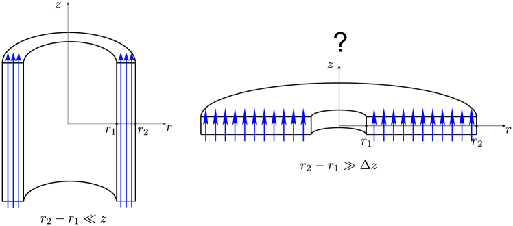
Figure 1: (a) Flow in a uniform magnetic field within a narrow gap between two cylinders. (b) A thin extended accretion disk in a uniform vertical magnetic field.

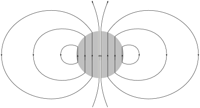
Figure 2: Deformation of a conducting sphere into a disk.The surface Lorentz force $\displaystyle\bm{j}_{\rm s}\times\bm{B}$ transforms the sphere into an elongated disk in the absence of other forces.

Let us discuss how to create a uniform magnetic field in an accretion disk (see Fig. 1). First, let us recall that this can be easily achieved in the case of two infinite, well-conducting cylinders (left in Fig. 1) with currents flowing in opposite directions. However, how can we organize currents in a flat conducting disk to obtain a uniform magnetic field inside it (right in Fig. 1)? To answer this question, let us consider the following problem. Suppose we have a well-conducting sphere with surface currents $\displaystyle j_{\phi}\propto\sin\theta$ such that the field inside the sphere is uniform. We smoothly deform the sphere into a disk while preserving the magnetic flux $\displaystyle{\rm d}\Phi_{\rm s}=B_{0}\,\cos\theta\,{\rm d}S$, where $\displaystyle{\rm d}S=2\pi R_{0}^{2}\,\sin\theta\,{\rm d}\theta$ is an element of the surface area of the sphere, and $\displaystyle\theta$ is the angle between the surface normal and the magnetic field lines. In the disk, we have $\displaystyle{\rm d}\Phi_{d}=B_{\rm d}2\pi r\,{\rm d}r$ ($\displaystyle B_{\rm d}$ being the field in the disk). Preserving the flux $\displaystyle\Phi_{\rm s}=\Phi_{\rm d}$ implies $\displaystyle 2\pi R_{0}^{2}\int B_{0}\,\sin\theta\,\cos\theta\,{\rm d}\theta=2\pi\int\,B_{\rm d}r\,{\rm d}r$. In the case of a uniform field, we have $\displaystyle R_{0}^{2}B_{0}\,\sin^{2}\theta+C=B_{\rm d}r^{2}$. The constant $\displaystyle C$ must be zero to satisfy the condition $\displaystyle\theta\to 0$, $\displaystyle r\to 0$. For uniform fields and $\displaystyle\theta=\pi/2$, we find the radius of the outer disk: $\displaystyle r_{\rm d}=R_{0}\sqrt{B_{0}/B_{\rm d}}$. Thus, we have constructed a disk with surface currents that induce a bending of the magnetic field lines on the surface and a uniform magnetic field inside.

Now let us remove a narrow region around the vertical axis from the considered sphere. Since the surface currents vanish near the vertical axis, removing a small region near the axis will not significantly alter the field inside the sphere. Of course, such an operation changes the topology: the sphere transforms into a torus.

Alternatively, the sphere can be deformed into a disk while preserving the magnetic flux, but with a radially variable magnetic field, $\displaystyle B_{\rm d}(r)$. During the deformation process, the changing magnetic field induces an electric field, which in turn strengthens or weakens the surface currents $\displaystyle\bm{j}_{\rm s}$ (Fig. 2). It should be evident that by deforming the sphere while conserving the magnetic flux, any desired dependence of the magnetic field on the radius can be obtained.

It is worth noting that in the obtained configuration, the surface current at the inner boundary of the disk becomes zero, and consequently, the Lorentz force acting on the surface element, $\displaystyle\bm{j}_{\rm s}\times\bm{B}$, also vanishes. At the outer boundary, as the magnetic field changes sign when transitioning from the disk to the outside, there is a jump in the magnetic field, and a surface current must flow. The Lorentz force will be determined by the sum of two forces acting on the surface current from the inner and outer magnetic fields. Since, by construction, the outer and inner fields are equal but oppositely directed near the boundary, the total Lorentz force applied to the outer boundary of the disk will be zero (Fig. 3).

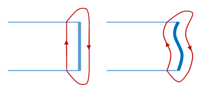
Figure 3: Schematic illustrating the cancellation of the Lorentz force $\displaystyle\bm{j}_{\rm s}\times\bm{B}$ at the outer boundary of the accretion disk. (a) Unperturbed configuration, with the surface current $\displaystyle\bm{j}_{\rm s}$ flowing perpendicular to the plane of the image. (b) The perturbed case, showing only the projection of the field onto the $\displaystyle r,z$ plane. The perturbed component of the field $\displaystyle b_{\phi}$ is not shown.

2.4 Differential equation for small perturbations

Following Velikhov (1959) and Chandrasekhar (1960), it is straightforward to show that in Eq. (16) $\displaystyle\omega^{2}$ must be a real number for a wide range of boundary conditions, i.e., only oscillations ($\displaystyle\omega^{2}>0$) or exponential growth or decay ($\displaystyle\omega^{2}<0$) of perturbations are allowed. It is convenient to eliminate the first derivative from  (16) using the substitution $\displaystyle\Psi=b_{r}\sqrt{r}$, in order to obtain a second-order differential equation:

$$\displaystyle\frac{{\rm d}^{2}\Psi}{{\rm d}r^{2}}+\left\{-k_{z}^{2}-\frac{3}{4}\frac{1}{r^{2}}+\frac{2\Omega\left[{\omega^{2}\,\varkappa^{2}}/(2\Omega\,k_{z}^{2})-c_{A}^{2}r\,({\rm d}\Omega/{\rm d}r)\right]}{\left(c_{A}^{2}-{\omega^{2}}/{k_{z}^{2}}\right)^{2}}\right\}\times$$

$$\displaystyle\times\,\Psi=0\,.$$ (17)

The boundary conditions for this equation are selected based on physical considerations, ensuring that the Lagrangian pressure perturbations vanish on the free boundary (recall that as shown earlier, the surface Lorentz force is zero on both boundaries):

$$\Delta p={\rm\delta}p+(\bm{\xi}\,\nabla)p=0,$$ (18)

where $\displaystyle\bm{\xi}$ is the vector of infinitesimal displacement and $\displaystyle{\rm\delta}p=p_{1}$ is the Eulerian pressure variation. In our problem formulation, Keplerian unperturbed flow is assumed, when the gravitational force is balanced by the centrifugal force, for small displacements $\displaystyle\bm{\xi}$, the second term in the expression for the Lagrangian variation can be neglected (up to terms of order $\displaystyle(h/r)^{2}$ in a thin accretion disk with semi-thickness $\displaystyle h$), and $\displaystyle\Delta p=p_{1}$. After dividing by the differential of time $\displaystyle{\rm d}t$, the equation (18) can be written as:

$$\frac{{\rm D}p}{{\rm D}t}=\frac{\partial p}{\partial t}+(\bm{u}\,\nabla)p=0\,,$$

where $\displaystyle{\rm D}/{\rm D}t$ represents the Lagrangian derivative, and $\displaystyle\partial/\partial t$ represents the Eulerian derivative.

At the outer and inner boundaries of the accretion disk with a magnetic field, the boundary conditions can be expressed as $\displaystyle p_{1}|_{r_{\mathrm{in}},r_{\mathrm{out}}}=0$. As implied by Eq. (13), these boundary conditions lead to homogeneous third-type boundary conditions for the function $\displaystyle\Psi$ at the flow boundaries $\displaystyle r_{\rm in},r_{\rm out}$:

$$\left.\frac{{\rm d}\Psi}{{\rm d}r}\right|_{r_{\rm in}}+\left.\frac{1}{2}\frac{\Psi}{r}\right|_{r_{\rm in}}=0\,,\quad\left.\frac{{\rm d}\Psi}{{\rm d}r}\right|_{r_{\rm out}}+\left.\frac{1}{2}\frac{\Psi}{r}\right|_{r_{\rm out}}=0\,.$$ (19)

It is worth noting that in the works of E.P. Velikhov (see Velikhov 1959 and Latter et al. 2015), a boundary value problem with homogeneous first-type conditions at the boundaries ($\displaystyle\Psi|_{r_{\mathrm{in}}}=0,\,\Psi|_{r_{\mathrm{out}}}=0$) was considered.

Equation (2.4) can be interpreted as a Schrödinger-like equation with ”energy”

$$E=-k_{z}^{2}$$ (20)

and ”potential”

$$U=\frac{3}{4}\frac{1}{r^{2}}-\frac{({\omega^{2}}/{k_{z}^{2}})\,\varkappa^{2}-c_{A}^{2}r\,({\rm d}\Omega^{2}/{{\rm d}r})}{\left(c_{A}^{2}-{\omega^{2}}/{k_{z}^{2}}\right)^{2}}\,.$$ (21)

As is well-known (see, for example, Landau and Lifshitz 1977; Flugge 1971), in the region of negative potential values $\displaystyle U$, there exist eigenvalues (”energy levels”) with negative energy $\displaystyle E<0$. The existence of levels with negative energy, i.e., solutions for $\displaystyle\bm{b}$, for real $\displaystyle k_{z}$ and $\displaystyle\omega^{2}<0$, indicates the instability of the flow. Thus, the form of the potential $\displaystyle U$ determines the region in the flow and the range of values of $\displaystyle\bm{B}$ that allow the development of MRI.

Let us highlight the properties of the potential $\displaystyle U$ that are relevant to our problem. For the Keplerian law with $\displaystyle\Omega^{2}=GM/r^{3}$ and $\displaystyle\varkappa^{2}=\Omega^{2}$, the potential takes the form:

$$U=\frac{3}{4}\frac{1}{r^{2}}-\frac{GM}{r^{3}}\,\frac{{\omega^{2}}/{k_{z}^{2}}+3c_{A}^{2}}{\left(c_{A}^{2}-{\omega^{2}}/{k_{z}^{2}}\right)^{2}}\,.$$ (22)

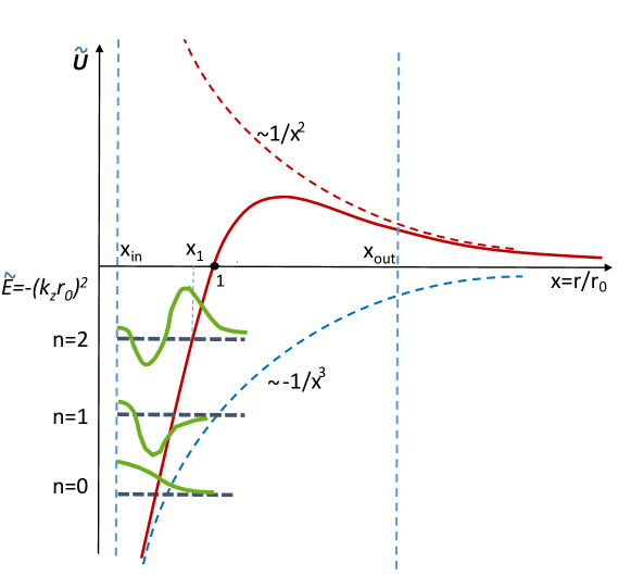
Figure 4: Schematic of the effective potential $\displaystyle\tilde{U}$ with characteristic points $\displaystyle x_{\mathrm{in}}$ (inner boundary of the flow), $\displaystyle x_{1}$ (turning point in the potential for a given energy level), $\displaystyle x=1$ (point where the potential becomes zero), and $\displaystyle x_{\mathrm{out}}$ (outer radius of the flow). The first three energy levels ($\displaystyle n=0,1,2$) and their corresponding eigenfunctions of the problem are shown in green color, in the case where $\displaystyle x_{\rm out}>1$.

For unstable modes ($\displaystyle\omega^{2}<0$), the numerator in the second term of equation (22) is positive only for perturbations with $\displaystyle\omega^{2}>-3c_{A}^{2}k_{z}^{2}$. Otherwise, the potential $\displaystyle U$ is strictly positive, and there are no stable states with negative energy. For $\displaystyle\omega^{2}<0$, the denominator in equation (22) does not vanish. In our problem (see Fig. 4), there are several characteristic points: the inner radius of the disk $\displaystyle r_{\mathrm{in}}$, the turning point $\displaystyle r_{1}$ for a given negative energy $\displaystyle E=-k_{z}^{2}$, the zero point of the potential $\displaystyle r_{0}$, and $\displaystyle r_{\mathrm{max}}=(3/2)r_{0}$, where the potential is maximal. It is evident that $\displaystyle r_{\mathrm{in}}\leq r_{1}\leq r_{0}$.

The potential turns to zero at the point

$$r_{0}=\frac{4}{3}\,G\,M\ \frac{{\omega^{2}}/{k_{z}^{2}}+3c_{A}^{2}}{\left(c_{A}^{2}-{\omega^{2}}/{k_{z}^{2}}\right)^{2}}=\frac{4}{3}\,\frac{G\,M}{c_{A}^{2}}\,\frac{{\omega^{2}}/{(k_{z}^{2}c_{A}^{2})}+3}{\left[1-{\omega^{2}}/({k_{z}^{2}c_{A}^{2}})\right]^{2}}\,.$$ (23)

It is convenient to introduce a dimensionless variable $\displaystyle x=r/r_{0}$. Then the dimensionless potential can be expressed as follows: Then the dimensionless potential can be written as

$$\tilde{U}=U\,r_{0}^{2}=\frac{3}{4}\frac{1}{x^{2}}-\frac{3}{4}\frac{1}{x^{3}}\,.$$ (24)

The dimensionless energy in the Schrödinger equation (2.4) is equal to

$$\tilde{E}=-k_{z}^{2}\,r_{0}^{2}\,.$$ (25)

The turning point of the potential $\displaystyle U$ is determined by the equation

$$-k_{z}^{2}-U(r_{1})=0\,$$ (26)

(see Fig. 4). Beyond the radius $\displaystyle r_{1}$, the perturbations decay quasi-exponentially. In dimensionless units, the turning point $\displaystyle x_{1}=r_{1}/r_{0}$ of the potential $\displaystyle\tilde{U}$ is determined by the equation:

$$4\tilde{E}x_{1}^{3}-3x_{1}+3=0,\quad x_{1}\leq 1\,.$$ (27)

For negative energy $\displaystyle\tilde{E}$, this cubic equation has one real root $\displaystyle x_{1}=r_{1}/r_{0}<1$:

$$x_{1}=\left(\frac{3}{-8\tilde{E}}\right)^{1/3}\left[\left(1-\sqrt{1-\frac{1}{9\tilde{E}}}\right)^{1/3}+\left(1+\sqrt{1-\frac{1}{9\tilde{E}}}\right)^{1/3}\right]\,.$$ (28)

Numerical solutions of Eq. (2.4) can be found in Appendix A. It should be noted that the global non-local analysis of MRI, leading to an equation of the form of a one-dimensional Schrödinger Eq. (2.4), has been investigated by Dubrulle and Knobloch (1993); Curry et al. (1994) with different boundary conditions.

2.5 Derivation of the dispersion equation and critical Alfvén velocity

Thus, in dimensionless variables, the problem reduces to a Sturm-Liouville problem for the equation

$$\Psi^{\prime\prime}-\tilde{U}\Psi+\tilde{E}\Psi=0$$ (29)

with the potential (24) and boundary conditions

$$\left.\frac{{\rm d}\Psi}{{\rm d}x}\right|_{x_{\rm in}}+\left.\frac{1}{2}\frac{\Psi}{x}\right|_{x_{\rm in}}=0,\quad\left.\frac{{\rm d}\Psi}{{\rm d}x}\right|_{x_{\rm out}}+\left.\frac{1}{2}\frac{\Psi}{x}\right|_{x_{\rm out}}=0\,.$$ (30)

Since the potential $\displaystyle\tilde{U}$ changes sign at $\displaystyle x=1$ ($\displaystyle r=r_{0}$), when solving this problem, it is necessary to distinguish between two cases: 1) the outer radius of the flow is located beyond the zero point of the potential $\displaystyle x_{\rm out}>1$ ($\displaystyle r_{\rm out}>r_{0}$), and 2) the flow terminates before reaching the zero point of the potential $\displaystyle x_{\rm out}<1$ ($\displaystyle r_{\rm out}<r_{0}$) (see details in Appendices A and B, respectively). From the solution of the boundary value problem, a discrete set of eigenvalues $\displaystyle\tilde{E}_{n}$, $\displaystyle n=0,1,2,\ldots$, is obtained,

$$\tilde{E}_{n}=-k_{z}^{2}r_{0}^{2}\,.$$ (31)

In the case of $\displaystyle x_{\rm out}>1$, the number $\displaystyle n$ corresponds to the number of zeros of the eigenfunctions on the interval between the inner boundary and the turning point of the potential for a given level $\displaystyle[x_{\rm in},x_{1}(\tilde{E}_{n})]$.

From Eq. (31), for each level with negative energy $\displaystyle\tilde{E}_{n}$, we obtain a dispersion equation

$$r_{0}=\frac{\sqrt{-\tilde{E}_{n}}}{k_{z}}=\frac{4}{3}\,\frac{GM}{c_{A}^{2}}\,\frac{{\omega^{2}}/({k_{z}^{2}c_{A}^{2}})+3}{\left[1-{\omega^{2}}/({k_{z}^{2}c_{A}^{2}})\right]^{2}}\,.$$ (32)

In dimensionless units normalized by $\displaystyle r_{0}$, Eq. (32) becomes a quadratic equation for the dimensionless quantity $\displaystyle{\omega^{2}}/({k_{z}^{2}c_{A}^{2}})$:

$$\frac{3}{4}\left(\frac{c_{A}}{v_{\phi}(r_{0})}\right)^{2}\left(1-\frac{\omega^{2}}{k_{z}^{2}c_{A}^{2}}\right)^{2}-\frac{\omega^{2}}{k_{z}^{2}c_{A}^{2}}-3=0\,,\quad v^{2}_{\phi}(r_{0})\equiv\frac{GM}{r_{0}}=\frac{GMk_{z}}{\sqrt{-\tilde{E}_{n}}}\,.$$ (33)

Its solution is as follows:

$$\omega^{2}=c_{A}^{2}k_{z}^{2}\,\left(1+\frac{1\pm\sqrt{1+12\left[{c_{A}}/{v_{\phi}(r_{0})}\right]^{2}}}{({3}/{2})\,\left[{c_{A}}/{v_{\phi}(r_{0})}\right]^{2}}\right)\,.$$ (34)

Note that this dispersion equation involves the flow velocity at radius $\displaystyle r_{0}$ and does not explicitly depend on the boundaries of the flow where the boundary conditions are satisfied; the boundary conditions determine the set of eigenvalues $\displaystyle\tilde{E}_{n}$.

The critical magnetic field corresponding to the neutral mode $\displaystyle\omega^{2}=0$ is given by:

$$\left(\frac{c_{A}}{v_{\phi}(r_{0})}\right)_{\mathrm{cr}}^{2}=4\,,$$ (35)

which can be rewritten as:

$$(c_{A})^{2}_{\mathrm{cr}}=\frac{4G\,M}{r_{0}}=\frac{4G\,M\,k_{z}}{\sqrt{-\tilde{E}_{n}}}\,.$$ (36)

Thus, in a sufficiently strong magnetic field, the shear flow is stabilized by the Lorentz force ($\displaystyle\omega^{2}=0$), as first noted by Velikhov (1959) for the case of flow in a narrow gap between two conducting cylinders.

Using Eq. (35), we rewrite Eq. (34) in the form:

$$\frac{\omega^{2}}{(c_{A})^{2}_{\mathrm{cr}}k_{z}^{2}}=\left(\frac{c_{A}}{(c_{A})_{\mathrm{cr}}}\right)^{2}\left(1+\frac{1\pm\sqrt{1+48\,({c_{A}}/{(c_{A})_{\mathrm{cr}}})^{2}}}{6\,({c_{A}}/{(c_{A})_{\mathrm{cr}}})^{2}}\right)\,.$$ (37)

Below, only the unstable modes with $\displaystyle\omega^{2}<0$ are considered, corresponding to the minus sign in Eq. (37). For small $\displaystyle\left(\frac{c_{A}}{(c_{A})_{\mathrm{cr}}}\right)^{2}\ll 1$, Eq. (37) can be approximated as

$$\frac{\omega^{2}}{(c_{A})^{2}_{\mathrm{cr}}k_{z}^{2}}\approx\left(\frac{c_{A}}{(c_{A})_{\mathrm{cr}}}\right)^{2}\left(-3+48\,\left(\frac{c_{A}}{(c_{A})_{\mathrm{cr}}}\right)^{2}\right)\,.$$ (38)

In other words, $\displaystyle\omega^{2}\to 0$ as $\displaystyle c_{A}^{2}\to 0$. This behavior of $\displaystyle\omega^{2}$ differs from the result of local analysis, where the MRI occurs even for arbitrarily small (but nonzero!) background magnetic field (see, for example, Shakura and Postnov 2015b).

It is evident that there exists a maximum growth rate of the MRI and its corresponding Alfvén speed (see Fig. 5):

$$\left(\frac{c_{A}}{(c_{A})_{\mathrm{cr}}}\right)^{2}_{\mathrm{max}}=\frac{5}{16},\qquad\frac{\omega^{2}}{(c_{A})^{2}_{\mathrm{cr}}k_{z}^{2}}=-\frac{3}{16}\,.$$ (39)

In real flows, there is always an inner radius $\displaystyle r_{\mathrm{in}}$. For sufficiently large outer radius $\displaystyle r_{\mathrm{out}}\gg r_{\mathrm{in}}$, it is possible to solve the problem exactly and find the eigenvalues $\displaystyle\tilde{E}_{n}=-k_{z}^{2}r_{0}^{2}$ (see Appendix A), from which the location of the zero point $\displaystyle r_{0}$ of the effective potential $\displaystyle U(r)$ can be calculated. In the quasi-classical approximation, the solution $\displaystyle\tilde{E}_{n}(x_{\mathrm{in}})$, where $\displaystyle x_{\mathrm{in}}=r_{\mathrm{in}}/r_{0}$, is expressed through the integral (85) (see Appendix A). Then, the position of $\displaystyle r_{0}$ in the flow can be calculated from the solution of the problem with a given $\displaystyle r_{\mathrm{in}}$ using the formula $\displaystyle r_{0}=r_{\mathrm{in}}/x_{\mathrm{in}}$. In the special case of small $\displaystyle k_{z}\approx 0$ (i.e., $\displaystyle\tilde{E}_{n}\approx 0$), there is an analytical solution (see (87), (88)):

$$r_{0}=r_{\mathrm{in}}\left\{\left[\frac{\pi}{\sqrt{3}}\left(n+\frac{3}{4}\right)+\frac{\pi}{2}\right]^{2}+1\right\}\,.$$ (40)

In the case of $\displaystyle r_{\mathrm{out}}<r_{0}$, the potential between the boundaries does not change sign, and the problem of finding the eigenvalues of Eq. (29) is simplified (see Appendix B).

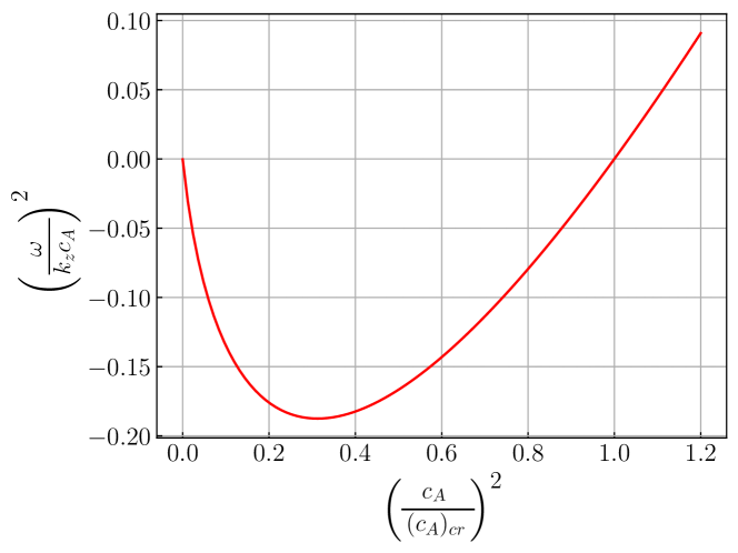
Figure 5: Solution of the dispersion equation (37) with a minus sign in front of the square root for unstable modes $\displaystyle\omega^{2}<0$.

2.6 Application to thin accretion disks

In accretion disks, the wavelength of perturbations $\displaystyle\lambda=2\pi/k_{z}$ in the vertical coordinate must be smaller the disk semi-thickness $\displaystyle h$. This condition limits the allowed ”energy levels.” Indeed, at the turning point $\displaystyle x_{1}$, we have

$$\tilde{E}=-k_{z}^{2}r_{0}^{2}=-4\pi^{2}\left(\frac{h}{\lambda}\right)^{2}\left(\frac{r_{1}}{h}\right)^{2}\frac{1}{x_{1}^{2}}\,.$$ (41)

Therefore, the requirement

$$\left(\frac{\lambda}{h}\right)^{2}=-\frac{4\pi^{2}}{x_{1}^{2}\tilde{E}}\left(\frac{r_{1}}{h}\right)^{2}<1$$ (42)

gives the permissible energy levels that satisfy the following condition:

$$x_{1}^{2}\,|\tilde{E}|>\frac{4\pi^{2}}{(h/r_{1})^{2}}\,.$$ (43)

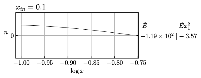
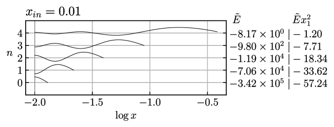
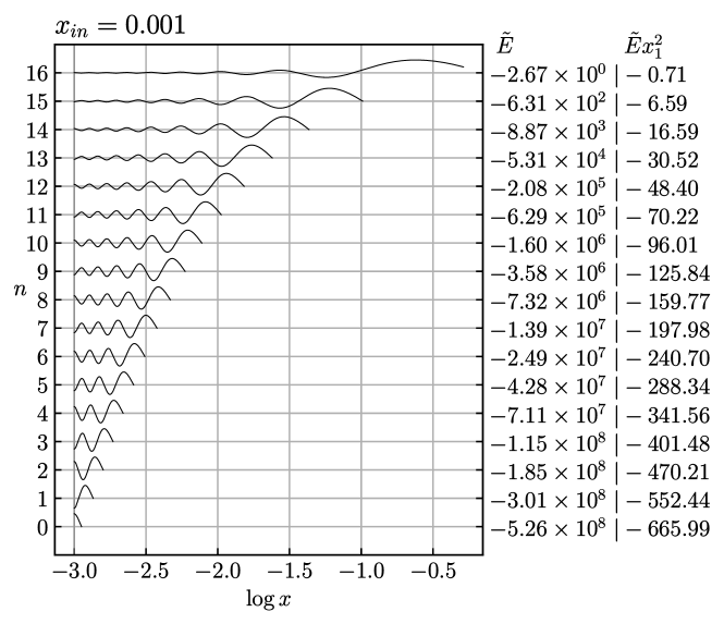
Figure 13: Normalized solutions of Eq. (79), plotted as $\displaystyle\Psi/\Psi_{\mathrm{max}}$, with the boundary condition (30), $\displaystyle\Psi^{\prime}|_{x_{\mathrm{in}}}+{\Psi}/({2x_{\mathrm{in}}})=0$ at $\displaystyle x_{\mathrm{in}}$, and (83) on $\displaystyle\Psi^{\prime}(x_{1})$ at $\displaystyle x_{1}$, corresponding to $\displaystyle\lim_{x\to\infty}\Psi(x)=0$, for $\displaystyle x_{\mathrm{in}}=10^{-1}$ (a), $\displaystyle 10^{-2}$ (b), and $\displaystyle 10^{-3}$ (c). As $\displaystyle x_{\mathrm{in}}$ decreases (indicating a deeper potential well), the number of stationary negative energy levels increases. The exponentially decaying part of the solution for $\displaystyle x>x_{1}$ is not shown.

For a typical value of the relative thickness of a geometrically thin disk, $\displaystyle h/r\lesssim 0.1$, in thin accretion disks, this yields $\displaystyle x_{1}^{2}|\tilde{E}|>4\times 10^{3}$. Considering that for large $\displaystyle|\tilde{E}|\gg 1$, $\displaystyle x_{1}\approx\left({3}/({4|\tilde{E}|})\right)^{1/3}$ (see Eq. (28)), the corresponding energy levels must have $\displaystyle|\tilde{E}|>7\times 10^{10}$. Such levels are only possible for very small $\displaystyle x_{\mathrm{in}}\ll 1$ (see Appendix A, Fig. 13).

The critical magnetic field, above which the MRI is suppressed, can be expressed in terms of the Keplerian velocity at the inner boundary of the flow, $\displaystyle v_{\phi}(r_{\mathrm{in}})$:

$$(c_{A})_{\mathrm{cr}}^{2}=\frac{4GM}{r_{0}}=x_{\mathrm{in}}\frac{4GM}{r_{\mathrm{in}}}=4x_{\mathrm{in}}v_{\phi}^{2}(r_{\mathrm{in}})\,.$$ (44)

It is easy to obtain an upper limit on the possible value of the dimensionless parameter $\displaystyle x_{\mathrm{in}}=r_{\mathrm{in}}/r_{0}$. Indeed, all possible energy levels can take values

$$-\tilde{E}_{n}=\frac{r_{\mathrm{in}}^{2}k_{z}^{2}}{x_{\mathrm{in}}^{2}}<-\tilde{U}(x_{\mathrm{in}})=\frac{3}{4}\frac{1}{x_{\mathrm{in}}^{3}}-\frac{3}{4}\frac{1}{x_{\mathrm{in}}^{2}}\,,$$ (45)

from which

$$x_{\mathrm{in}}<\frac{1}{1+({4}/{3})\,r_{\mathrm{in}}^{2}\,k_{z}^{2}}\,.$$ (46)

Note that this inequality gives an obvious upper limit $\displaystyle x_{\mathrm{in}}<1$ for $\displaystyle k_{z}\to 0$, while as shown in Appendix A, energy levels with $\displaystyle n=0$ exist only when $\displaystyle x_{\mathrm{in}}<0.8116$. Substituting inequality (46) into (44), we obtain an upper limit for the critical magnetic field:

$$(c_{A})_{\mathrm{cr}}^{2}<\frac{4v_{\phi}^{2}(r_{\mathrm{in}})}{1+({4}/{3})\,r_{\mathrm{in}}^{2}k_{z}^{2}}\,.$$ (47)

Using the condition for thin disks with the wavelength of perturbations in the $\displaystyle z$-coordinate $\displaystyle\lambda/h=2\pi/(k_{z}h)<1$ and considering $\displaystyle h/r_{\mathrm{in}}<1$, we transform (47) into the form:

$$\frac{(c_{A})_{\mathrm{cr}}}{v_{\phi}(r_{\mathrm{in}})}<\frac{\sqrt{3}}{2\pi}\left(\frac{h}{r_{\mathrm{in}}}\right)\sqrt{\frac{\lambda}{h}},\quad\frac{(c_{A})_{\mathrm{cr}}}{c_{s}(r_{\mathrm{in}})}<\frac{\sqrt{3}}{2\pi}\sqrt{\frac{\lambda}{h}}\,.$$ (48)

(In the last inequality, we used the relation between the Keplerian velocity and the sound speed at the inner boundary of the thin accretion disk $\displaystyle c_{s}(r_{\mathrm{in}})=v_{\phi}(r_{\mathrm{in}})(h/r_{\mathrm{in}})$.)

Thus, in thin accretion disks, MRI perturbations with a wavelength $\displaystyle\lambda<h$ in the $\displaystyle z$-coordinate can be significantly suppressed.

Depending on the type of accretor (regular stars or relativistic compact objects), the inner radius of the flow can vary greatly from a few tens to millions of kilometers, while the outer radius is determined by the physical situation, such as being limited by the size of the Roche lobe in the case of binary systems. Since in thin disks $\displaystyle h/r\sim 0.05$, the upper limit of the critical magnetic field that suppresses MRI in thin disks (48) is $\displaystyle\sim 1/\sqrt{r_{\mathrm{in}}}$ and significantly differs for different types of accretors.

Previous studies on the critical magnetic field for suppressing MRI in the context of global analysis with different boundary conditions can be found, for example, in Papaloizou and Szuszkiewicz (1992); Latter et al. (2015). Papaloizou and Szuszkiewicz (1992) derived the critical magnetic field using the energy method. Only an upper estimate was obtained, according to which (equation (41) in the cited work) the critical magnetic field in thin disks is determined by the Alfvén velocity, which is equal to the Keplerian velocity of the flow multiplied by the square root of the ratio of the disk’s semi-thickness to its radius. It should also be noted that the critical Alfvén velocity in the local analysis by Balbus and Hawley (1991) is, to within a multiplicative factor, equal to the Keplerian velocity multiplied by the ratio of the wavelength of a perturbation in the $\displaystyle z$-coordinate to the radius. As can be seen from the comparison of these statements with (48), our result provides a much more definite value for the critical field.

3 MRI with radially dependent Alfvén velocity

Until now, our consideration of MRI has been limited to the case of a constant background Alfvén velocity. However, in real astrophysical situations, the Alfvén velocity should decrease with radius at least as fast as the angular velocity of the flow or even faster. Below, we will consider two cases: (1) $\displaystyle c_{A}^{2}$ depends on radius as $\displaystyle v_{\phi}^{2}\propto 1/r$ due to the variable density with a constant background magnetic field, and (2) $\displaystyle c_{A}^{2}\propto 1/r^{q}$ for a variable background magnetic field with the density constant over radius.

3.1 Case of constant background magnetic field

The square of the Alfvén velocity can decrease linearly with radius when the background magnetic field is constant, but the density of the flow increases linearly with radius. It should be noted that the density varying with radius still implies the use of the continuity equation in the form of Eq. (5). Let us rewrite Eq. (1) as follows:

$$\frac{1}{\rho}\left(\frac{\partial\rho}{\partial t}+\bm{u}\,\bm{\nabla}\rho\right)+\bm{\nabla}\,\bm{u}=\frac{{\rm D}\ln\rho}{{\rm D}t}+\bm{\nabla}\,\bm{u}=0.$$

Now, locally, the density $\displaystyle\rho$ varies (Eulerian derivative $\displaystyle\partial\rho/\partial t\neq 0$), but the substantial (Lagrangian) derivative of density with time $\displaystyle{\rm D}\rho/{\rm D}t=\partial\rho/\partial t+\bm{u}\,\bm{\nabla}\rho=0$, $\displaystyle{\rm D}\ln\rho/{\rm D}t=0$. Thus, for an incompressible fluid in the case of density varying with coordinates, the continuity equation becomes $\displaystyle\bm{\nabla}\,\bm{u}=0$ (Landau and Lifshitz, 1959; Acheson, 1990). Therefore, for a variable background density $\displaystyle\rho_{0}$, equations (5–12) for linear perturbations remain unchanged. However, instead of the potential Eq. (22) with $\displaystyle c_{A}^{2}=\mathrm{const}$, the effective potential takes the form

$$\displaystyle U_{e}=\frac{3}{4}\frac{1}{r^{2}}-\frac{GM}{r^{3}c_{A}^{2}}\frac{{\omega^{2}}/({k_{z}^{2}c_{A}^{2}})+3}{\left[1-{\omega^{2}}/({k_{z}^{2}c_{A}^{2}})\right]^{2}}=$$

$$\displaystyle=\frac{3}{4}\frac{1}{r^{2}}-\frac{GM}{r^{3}}\frac{{\omega^{2}}/{k_{z}^{2}}+3\epsilon v_{\phi}^{2}(r)}{\left[\epsilon v_{\phi}^{2}(r)-{\omega^{2}}/{k_{z}^{2}}\right]^{2}}\,.$$ (49)

Here $\displaystyle\epsilon\equiv c_{A}^{2}/v_{\phi}^{2}=\mathrm{const}$ is a parameter. The potential (3.1) has the same characteristic points as in the previous case (see Section 2.4): $\displaystyle r_{0}$, where $\displaystyle U_{e}(r_{0})=0$, the turning point $\displaystyle r_{1}$, where $\displaystyle E-U_{e}(r_{1})=0$, and the inner radius of the flow $\displaystyle r_{\mathrm{in}}$.

The potential $\displaystyle U_{e}$ becomes zero at the point

$$r_{0}=\frac{4}{3}\,G\,M\,\frac{{\omega^{2}}/{k_{z}^{2}}+3\epsilon v_{\phi}^{2}(r_{0})}{\left[\epsilon v_{\phi}^{2}(r_{0})-{\omega^{2}}/{k_{z}^{2}}\right]^{2}}\,.$$ (50)

From the last equation, we obtain the dispersion equation $\displaystyle\omega(k_{z})$:

$$\frac{3}{4}\,\epsilon\,\left(1-\frac{\omega^{2}}{k_{z}^{2}\epsilon\,v_{\phi}^{2}(r_{0})}\right)^{2}-\frac{\omega^{2}}{k_{z}^{2}\,\epsilon\,v_{\phi}^{2}(r_{0})}-3=0$$ (51)

with the solution

$$\omega^{2}=\epsilon\,v_{\phi}^{2}(r_{0})\,k_{z}^{2}\,\left(1+\frac{1\pm\sqrt{1+12\epsilon}}{{3\epsilon}/{2}}\right)\,.$$ (52)

The unstable MRI mode corresponds to the minus sign before the square root. As in Section 2.5, the critical magnetic field corresponds to the neutral mode $\displaystyle\omega^{2}=0$:

$$\epsilon_{\mathrm{cr}}=\left(\frac{c_{A}(r_{0})}{v_{\phi}(r_{0})}\right)^{2}=4\,.$$ (53)

For small $\displaystyle\epsilon\ll 1$,

$$\omega^{2}\approx\epsilon\,v^{2}_{\phi}(r_{0})\,k_{z}^{2}\,\left(-3+\epsilon\right)\,.$$ (54)

It can be seen that Eq. (52) yields the same maximum growth rate of MRI and the corresponding value of the Alfvén velocity as before (cf. Eq. (39)):

$$\epsilon=\left(\frac{c_{A}(r_{0})}{v_{\phi}(r_{0})}\right)_{\mathrm{max}}^{2}=\frac{5}{4}\,,\qquad\omega^{2}_{\mathrm{max}}=-\frac{3}{4}\,k_{z}^{2}\,v_{\phi}^{2}(r_{0})\,.$$ (55)

Clearly, the critical Alfvén velocity is the same as derived earlier (see Eq. (35)).

Now let us consider the turning point $\displaystyle r_{1}$ in the potential $\displaystyle U_{e}$, determined by the equation $\displaystyle-k_{z}^{2}-U_{e}(r_{1})=0$. In dimensionless variables $\displaystyle\tilde{E}=-k_{z}^{2}\,r_{0}^{2}$ and $\displaystyle x=r/r_{0}$, the equation for $\displaystyle x_{1}$ reads:

$$\tilde{E}-\tilde{U}_{e}=\tilde{E}-\frac{3}{4}\frac{1}{x_{1}^{2}}+\frac{1}{\epsilon x_{1}^{2}}\frac{3+K(\epsilon)}{[1-x_{1}\,K(\epsilon)]^{2}}=0\,,$$ (56)

where

$$K(\epsilon)=\frac{\omega^{2}}{k_{z}^{2}\,c_{A}^{2}(r_{0})}=1+\frac{1-\sqrt{1+12\epsilon}}{{3\epsilon}/{2}}\,.$$ (57)

It should be noted that the ”attractive” part of the potential in Eq. (56) depends on the parameter $\displaystyle\epsilon$. Also, in this case, for small $\displaystyle x\ll 1$, the ”repulsive” potential behaves as $\displaystyle 1/x^{2}$ compared to $\displaystyle 1/x^{3}$ in the case of Eq. (24). Eq. (56) is a fourth-degree equation for $\displaystyle x_{1}$ (in contrast to the cubic equation Eq. (27) for $\displaystyle x_{1}$ in the case of constant $\displaystyle c_{A}^{2}$). For small $\displaystyle x_{1}\ll 1$, the solution takes the form:

$$x_{1}^{2}\approx-\frac{3}{\tilde{E}}\left(\frac{1}{4}+\frac{1}{\epsilon}\right)$$ (58)

(cf. Eq. (28) for constant Alfvén velocity).

3.2 Case of radially dependent background magnetic field

If the background magnetic field depends on the radius, $\displaystyle\bm{B}=(0,0,B_{z}(r))$, the linearized MHD equations become more complex. The radial and vertical components of the Euler equations 7 and 9 are now expressed as follows, respectively:

$$\mathrm{i}\omega u_{r}-2\Omega u_{\phi}=-{\frac{1}{\rho_{0}}\frac{\partial p_{1}}{\partial r}}-\frac{1}{4\pi\rho_{0}}\left[\displaystyle\frac{\partial(b_{z}B_{z})}{\partial r}+\mathrm{i}k_{z}b_{r}B_{z}\right]\,,$$ (59)

$$\mathrm{i}\omega u_{z}=\mathrm{i}k_{z}\frac{p_{1}}{\rho_{0}}+\frac{1}{4\pi\rho_{0}}b_{r}\displaystyle\frac{\partial B_{z}}{\partial r}\,.$$ (60)

The vertical component of the induction equation  (12) turns into

$$\mathrm{i}\omega b_{z}=-\frac{1}{r}\displaystyle\frac{\partial(ru_{r}B_{z})}{\partial r}\,.$$ (61)

Following a similar procedure as in Section 2.4, after some algebraic manipulations, we obtain the equation for $\displaystyle b_{r}$ in the form:

$$\displaystyle\left(c_{A}^{2}-\frac{\omega^{2}}{k_{z}^{2}}\right)\,\left[\frac{\partial^{2}b_{r}}{\partial r^{2}}+\frac{\partial}{\partial r}\left(\frac{b_{r}}{r}\right)-b_{r}k_{z}^{2}\right]+$$

$$\displaystyle\frac{2\,\Omega\,\left[{\omega^{2}\,\varkappa^{2}}/({2\,\Omega\,k_{z}^{2}})-c_{A}^{2}\,r\,({{\rm d}\Omega}/{{\rm d}r})\right]}{c_{A}^{2}-{\omega^{2}}/{k_{z}^{2}}}\,b_{r}=$$

$$\displaystyle\frac{\partial c_{A}^{2}}{\partial r}\,\Bigg{\{}-\frac{b_{r}}{2r}-\frac{1}{2}\frac{\partial b_{r}}{\partial r}+\frac{\omega^{2}}{k_{z}^{2}c_{A}^{2}}\times$$

$$\displaystyle\times\left[-\frac{b_{r}}{2r}-\frac{\partial b_{r}}{\partial r}-\frac{1}{2}\frac{\partial^{2}c_{A}^{2}/\partial r^{2}}{\partial c_{A}^{2}/\partial r}\,b_{r}+\frac{3}{4c_{A}^{2}}\,\frac{\partial c_{A}^{2}}{\partial r}\,b_{r}\right]\Bigg{\}}\,.$$ (62)

The r.h.s. of the above equation vanishes for $\displaystyle c_{A}^{2}=$const. Here, we will consider the case of a power-law dependence of the Alfvén velocity on radius. Substituting $\displaystyle c_{A}^{2}\propto r^{-q}$ into Eq. (3.2), we obtain, for Keplerian flow ($\displaystyle\varkappa^{2}=\Omega^{2}=GM/r^{3}$), the following expression:

$$\displaystyle\frac{\partial^{2}b_{r}}{\partial r^{2}}+\left[1-q\,\frac{{c_{A}^{2}}/{2}+{\omega^{2}}/{k_{z}^{2}}}{c_{A}^{2}-\omega^{2}/k_{z}^{2}}\right]\,\frac{\partial}{\partial r}\left(\frac{b_{r}}{r}\right)+$$

$$\displaystyle+b_{r}\Bigg{\{}-k_{z}^{2}+\frac{G\,M}{r^{3}}\,\frac{{\omega^{2}}/{k_{z}^{2}}+3c_{A}^{2}}{\left(c_{A}^{2}-{\omega^{2}}/{k_{z}^{2}}\right)^{2}}+$$

$$\displaystyle+\frac{q}{r^{2}}\frac{\left(-{q}/{4}-1\right)\,{\omega^{2}}/{k_{z}^{2}}-c_{A}^{2}}{c_{A}^{2}-{\omega^{2}}/{k_{z}^{2}}}\Bigg{\}}=0\,.$$ (63)

Eq. (3.2) can be rewritten as

$$\displaystyle b_{r}^{\prime\prime}+g(r)\,b_{r}^{\prime}+f(r)=0\,,$$ (64)

$$\displaystyle g(r)=\frac{1}{r}\frac{1-{q}/{2}-(q+1)\,{\omega^{2}}/\left({k_{z}^{2}c_{A}^{2}}\right)}{1-{\omega^{2}}/\left({k_{z}^{2}c_{A}^{2}}\right)}\,,$$ (65)

$$\displaystyle f(r)=-k_{z}^{2}+\frac{G\,M}{c_{A}^{2}r^{3}}\,\frac{{\omega^{2}}/\left({k_{z}^{2}c_{A}^{2}}\right)+3}{\left[1-{\omega^{2}}/\left({k_{z}^{2}c_{A}^{2}}\right)\right]^{2}}-$$

$$\displaystyle-\frac{g(r)}{r}+\frac{q}{r^{2}}\frac{\left(-{q}/{4}-1\right)\,{\omega^{2}}/\left({k_{z}^{2}c_{A}^{2}}\right)-1}{1-{\omega^{2}}/\left({k_{z}^{2}c_{A}^{2}}\right)}\,.$$ (66)

The first derivative can be excluded in a standard way by the substitution $\displaystyle z=b_{r}\exp\left[-{1}/{2}\int^{r}g(s)\,{\rm d}s\right]$, yielding the equation

$$z^{\prime\prime}+\left(f-\frac{g^{\prime}}{2}-\frac{g^{2}}{4}\right)z=0\,.$$ (67)

Substituting the functions $\displaystyle f$ and $\displaystyle g$ into Eq. (67), we obtain the equation:

$$\displaystyle z^{\prime\prime}+\Bigg{\{}-k_{z}^{2}-\frac{3}{4}\frac{1}{r^{2}}-\frac{q}{r^{2}}\,\frac{{q}/{16}+{1}/{2}-\left(q/4+1/2\right)\,{\omega^{2}}/\left(k_{z}^{2}c_{A}^{2}\right)}{\left[1-{\omega^{2}}/\left({k_{z}^{2}c_{A}^{2}}\right)\right]^{2}}+$$

$$\displaystyle+\,\frac{G\,M}{c_{A}^{2}r^{3}}\,\frac{{\omega^{2}}/\left({k_{z}^{2}c_{A}^{2}}\right)+3}{\left[1-{\omega^{2}}/\left({k_{z}^{2}c_{A}^{2}}\right)\right]^{2}}\Bigg{\}}\,z=0\,.$$ (68)

Clearly, it reduces to Eq. (2.4) for $\displaystyle q=0$. for the case of a constant magnetic field. For the case when $\displaystyle q\neq 0$, the effective potential in the Schrödinger-like Eq. (68) reads:

$$\displaystyle U_{q}=\frac{3}{4}\frac{1}{r^{2}}+\frac{q}{r^{2}}\,\frac{{q}/{16}+{1}/{2}-\left({q}/{4}+{1}/{2}\right)\,{\omega^{2}}/\left({k_{z}^{2}c_{A}^{2}}\right)}{\left[1-{\omega^{2}}/\left({k_{z}^{2}c_{A}^{2}}\right)\right]^{2}}-$$ (69)

$$\displaystyle-\,\frac{GM}{c_{A}^{2}r^{3}}\,\frac{{\omega^{2}}/\left({k_{z}^{2}c_{A}^{2}}\right)+3}{\left[1-{\omega^{2}}/\left({k_{z}^{2}c_{A}^{2}}\right)\right]^{2}}\,.$$

Foe each value of $\displaystyle q$, the potential $\displaystyle U_{q}$ becomes zero at:

$$\displaystyle r_{0}=\frac{GM}{c_{A}^{2}}\times$$

$$\displaystyle\times\frac{{\omega^{2}}/\left({k_{z}^{2}c_{A}^{2}}\right)+3}{({3}/{4})\left[1-{\omega^{2}}/\left({k_{z}^{2}c_{A}^{2}}\right)\right]^{2}-\left({q^{2}}/{4}+{q}/{2}\right){\omega^{2}}/\left({k_{z}^{2}c_{A}^{2}}\right)+\left({q^{2}}/{16}+{q}/{2}\right)}\,.$$

The dispersion equation at the point $\displaystyle r_{0}$ reads:

$$\displaystyle\frac{\omega^{2}}{k_{z}^{2}c_{A}^{2}(r_{0})}=1+\frac{q}{3}+\frac{q^{2}}{6}+\frac{2}{3}\,\left(\frac{v_{\phi}(r_{0})}{c_{A}(r_{0})}\right)^{2}\pm$$

$$\displaystyle\pm\sqrt{\left(\frac{q^{2}}{6}+\frac{q}{3}+\frac{2}{3}\left(\frac{v_{\phi}(r_{0})}{c_{A}(r_{0})}\right)^{2}\right)^{2}+\frac{16}{3}\left(\frac{v_{\phi}(r_{0})}{c_{A}(r_{0})}\right)^{2}+\frac{q^{2}}{4}}.$$ (71)

The unstable MRI mode corresponds to the minus sign before the square root. The zero mode $\displaystyle\omega^{2}=0$ occurs at the critical magnetic field

$$\epsilon_{cr}\equiv\left(\frac{c_{A}(r_{0})}{v_{\phi}(r_{0})}\right)_{\mathrm{cr}}^{2}=\frac{48}{12+8q+q^{2}}\,.$$ (72)

Using the identity

$$\left(\frac{v_{\phi}}{c_{A}}\right)^{2}=\left(\frac{v_{\phi}}{(c_{A})_{\mathrm{cr}}}\right)^{2}\left(\frac{(c_{A})_{\mathrm{cr}}}{c_{A}}\right)^{2}\,,$$ (73)

we rewrite the dispersion equation 3.2 in the form similar to Eq. (37), as a function of a dimensionless value $\displaystyle\left({(c_{A})_{\mathrm{cr}}}/{c_{A}}\right)^{2}$:

$$\displaystyle\frac{\omega^{2}}{(c_{A})^{2}_{\mathrm{cr}}k_{z}^{2}}=\left(\frac{c_{A}}{(c_{A})_{\mathrm{cr}}}\right)^{2}\left[1+\frac{q}{3}+\frac{q^{2}}{6}+\frac{2}{3}\,\left(\frac{v_{\phi}}{c_{A}}\right)^{2}\right.\pm$$

$$\displaystyle\left.\pm\sqrt{\left(\frac{q^{2}}{6}+\frac{q}{3}+\frac{2}{3}\left(\frac{v_{\phi}}{c_{A}}\right)^{2}\right)^{2}+\frac{16}{3}\left(\frac{v_{\phi}}{c_{A}}\right)^{2}+\frac{q^{2}}{4}}\,\right].$$ (74)

(see Fig. 6). In Eq. (3.2), value $\displaystyle\left({v_{\phi}}/{c_{A}}\right)^{2}$ can be expressed in terms of Eqs. (72) and (73).

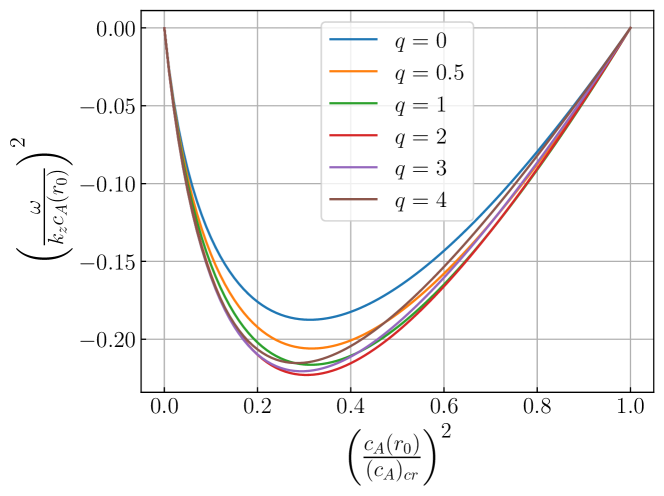
Figure 6: MRI dispersion curves described by Eq. (3.2) for various values of $\displaystyle q$. In the limit of $\displaystyle c_{A}/(c_{A})_{\mathrm{cr}}\ll 1$, the dispersion equation takes the form of Eq. (38) for all values of $\displaystyle q$.

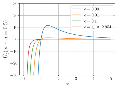
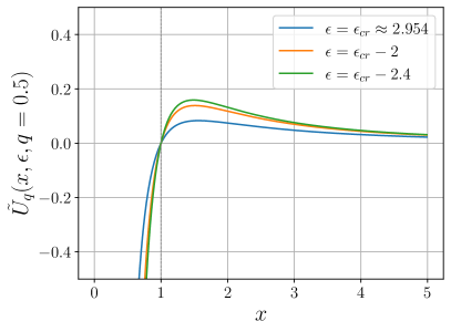
Figure 7: The effective potential $\displaystyle\tilde{U}_{q}(x,\epsilon,q)$ described by Eq. (3.2) for $\displaystyle q=0.5$ and various values of the parameter $\displaystyle\epsilon=c_{A}^{2}(r_{0})/v_{\phi}^{2}(r_{0})$. The critical value $\displaystyle\epsilon_{\mathrm{cr}}$ is determined from Eq. (72).

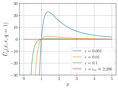
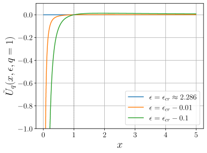
Figure 8: The same as in Fig. 7, for $\displaystyle q=1$.

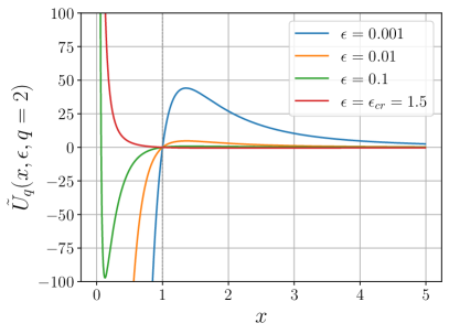
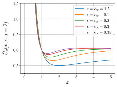
Figure 9: The same as in Fig. 7, for $\displaystyle q=2$.

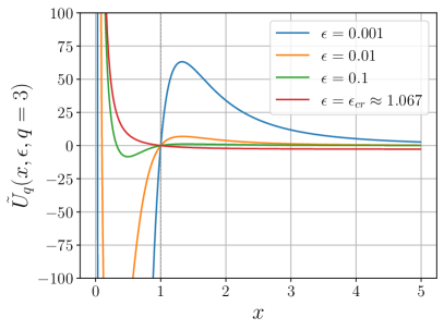
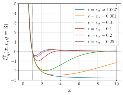
Figure 10: The same as in Fig. 7, for $\displaystyle q=3$.

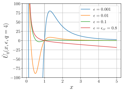
Figure 11: The same as in Fig. 7, for $\displaystyle q=4$.

Let us use, as above, the dimensionless variables $\displaystyle x=r/r_{0}$, $\displaystyle c_{A}^{2}=c_{A}^{2}(r_{0})x^{-q}$, parameter $\displaystyle\epsilon=c_{A}^{2}(r_{0})/v_{\phi}^{2}(r_{0})$ and denote the r.h.s. of Eq. (3.2) $\displaystyle{\omega^{2}}/\left({k_{z}^{2}c_{A}^{2}(r_{0})}\right)=K(\epsilon)$. Then the dimensionless potential $\displaystyle\tilde{U}_{q}=U_{q}r_{0}^{2}$ is as follows

$$\displaystyle\tilde{U}_{q}(x,\epsilon,q)=\frac{1}{x^{2}}\,\left(\frac{3}{4}+\frac{q^{2}/16+{q}/{2}-K(\epsilon)\,x^{q}\,({q^{2}}/{4}+{q}/{2})}{(1-K(\epsilon)x^{q})^{2}}\right)-$$

$$\displaystyle\frac{1}{x^{3-q}}\,\frac{3+K(\epsilon)\,x^{q}}{\epsilon\,(1-K(\epsilon)\,x^{q})^{2}}\,.$$ (75)

It should be noted that in the case of $\displaystyle q\neq 0$, both the ”repulsive” and ”attractive” parts of the effective potential depend on $\displaystyle\epsilon$.

Let us discuss some features of the potential $\displaystyle\tilde{U}_{q}$.

1. By construction, $\displaystyle\tilde{U}_{q}(1,\epsilon,q)=0$ for any $\displaystyle\epsilon,q$.

2. For $\displaystyle\epsilon\to\epsilon_{\mathrm{cr}}$, see Eq. (72), $\displaystyle K(\epsilon)\to 0$:

   $$\tilde{U}_{q}(x,\epsilon\to\epsilon_{\mathrm{cr}},q)=\left(\frac{3}{4}+\frac{q^{2}}{16}+\frac{q}{2}\right)\left(\frac{1}{x^{2}}-\frac{1}{x^{3-q}}\right)\,.$$ (76)

   The potential $\displaystyle\tilde{U}_{q}(x,\epsilon\to\epsilon_{\mathrm{cr}},q=1)=0$ for any $\displaystyle x$. For $\displaystyle q<1$, $\displaystyle\tilde{U}_{q}$ changes sign from negative to positive at $\displaystyle x=1$, and vice versa for $\displaystyle q>1$.

3. For $\displaystyle q<1$, there exists only one zero point of the potential: $\displaystyle\tilde{U}_{q}(x=1,\epsilon,q<1)=0$.

4. For $\displaystyle q>1$, the second zero point $\displaystyle x_{2}$ appears at $\displaystyle x<1$ with $\displaystyle\lim_{\epsilon\to 0}x_{2}=0$ and $\displaystyle\lim_{x\to 0}\tilde{U}_{q}(x,\epsilon,q)\to+\infty$. That is, the potential reaches a minimum at a certain point $\displaystyle x_{\min}$: $\displaystyle x_{2}<x_{\min}<1$.

These features of the effective potential $\displaystyle\tilde{U}_{q}$ for different values of $\displaystyle q$ and $\displaystyle\epsilon$ are shown in Fig. 7-11. It can be seen that for $\displaystyle q\leq 1$, the effective potential $\displaystyle\tilde{U}_{q}$ has the same shape as for $\displaystyle q=0$ (see Fig. 4), and the analysis of the MRN modes remains unchanged. For $\displaystyle q>1$, a minimum of the effective potential appears with $\displaystyle x_{2}<x_{\min}<1$, and the unstable energy levels should be sought between the two turning points for the corresponding effective energies $\displaystyle\tilde{E}=-k_{z}r_{0}^{2}$. In contrast to the $\displaystyle q=0$ case, there exists a minimum energy $\displaystyle\tilde{E}_{\min}=\tilde{U}_{q}(x_{\min},\epsilon,q)$.

It is important to note that for cases with $\displaystyle q>1$ and $\displaystyle x_{\mathrm{in}}\ll 1$, there can be two turning points in the effective potential $\displaystyle\tilde{U}_{q}$ for the energy levels $\displaystyle\tilde{E}=-k_{z}^{2}r_{0}^{2}$ ($\displaystyle[x_{1}]_{\min}$ and $\displaystyle[x_{1}]_{\max}$). It is also possible that $\displaystyle\tilde{E}<[\tilde{U}_{q}]_{\min}$, and stable negative energy levels (corresponding to MRN modes) do not exist. If the dimensionless radius of the inner disk $\displaystyle x_{\mathrm{in}}$ falls between the roots of the effective potential $\displaystyle\tilde{U}_{q}$, then a free boundary of the flow occurs at the point $\displaystyle x_{\mathrm{in}}$, as in the previously considered $\displaystyle q=0$ case.

Thus, the analysis of the shape of the effective potential $\displaystyle\tilde{U}_{q}$ indicates the need to take it into account when considering global MRN in specific physical cases.

4 Summary and discussion

4.1 Non-local modal analysis with constant background magnetic field.

We have revisited the development of MRI in Keplerian flows of ideal fluid. We have shown that taking into account radial nonlocality in the analysis of perturbations in the form of $\displaystyle f(r)\,e^{\mathrm{i}(\omega t-k_{z}z)}$ leads to the appearance of the term $\displaystyle-({3}/{4})\,({1}/{r^{2}})$ in Eq. (2.4) for small perturbations. The equation for small perturbations takes the form of a stationary Schrödinger equation with an effective potential that determines (in the form of a dispersion equation) the region of negative $\displaystyle\omega^{2}$ values–the region of MRI growth. The neutral mode $\displaystyle\omega^{2}=0$ corresponds to the critical magnetic field (36). The critical field in terms of the Alfvén velocity $\displaystyle c_{A}^{2}$ is given by $\displaystyle(c_{A})_{\mathrm{cr}}^{2}=4GM/r_{0}$, where $\displaystyle r_{0}$ is the zero point of the potential $\displaystyle U$ (22) in Eq. (2.4).

The second important result is the significant reduction (compared to the local analysis) of the MRI instability increment for the case of $\displaystyle c_{A}^{2}\ll(c_{A})_{\mathrm{cr}}^{2}$ (see Eq. (38)). Indeed, neglecting the term $\displaystyle-\frac{3}{4}\frac{1}{r^{2}}$ in the equation 2.4 and replacing the derivative $\displaystyle\frac{\partial}{\partial r}\to-ik_{r}$, the equation 2.4 transforms into a fourth-degree algebraic equation with the solution

$$\omega^{2}=\left(\frac{k_{z}}{k}\right)^{2}\left[c_{A}^{2}k_{z}^{2}+\frac{\Omega^{2}}{2}-\sqrt{\frac{\Omega^{4}}{4}+4\Omega^{2}c_{A}^{2}k^{2}}\,\right]$$ (77)

(here $\displaystyle k^{2}=k_{r}^{2}+k_{z}^{2}$). The maximal instability increment in this case is independent of the magnetic field strength:

$$\omega^{2}_{\mathrm{max}}=-\frac{9}{16}\left(\frac{k_{z}}{k}\right)^{2}\Omega^{2}\,.$$ (78)

We stress the difference between the local result (78) and the nonlocal result (39). In the nonlocal approach, a critical magnetic field that suppresses MRI appears, which was absent in the local modal analysis (see, for example, Balbus and Hawley (1991); Shakura and Postnov (2018)). In the global analysis, the maximum increment of MRI is achieved at a specific value of the Alfvén velocity, $\displaystyle(c_{A}/(c_{A})_{\rm cr})^{2}=5/16$ (see Fig. 5 and Eq. (39)). The fact that MRI arises only in sufficiently weak magnetic fields was already noted in the seminal work by Balbus and Hawley (1991) (see also, for example, subsequent studies Salmeron et al. (2007); Bai and Stone (2013), etc.). For small magnetic fields, $\displaystyle c_{A}\ll(c_{A})_{\mathrm{cr}}$, the instability increment is suppressed by a factor of $\displaystyle 3\,(c_{A}/(c_{A})_{\mathrm{cr}})$, as shown by Eq. (38).

We emphasize that, as shown by numerical analysis (see Appendix A), in ”shallow” potential wells with the dimensionless inner radius of the flow $\displaystyle x_{\mathrm{in}}=r_{\mathrm{in}}/r_{0}>0.8$, there are no stationary eigenmodes 2.4, i.e., MRI is absent there. For $\displaystyle x_{\mathrm{in}}=r_{\mathrm{in}}/r_{0}<0.8$, stationary levels arise, corresponding to very small $\displaystyle k_{z}$ and large perturbation wavelengths. The number of stationary levels increases as $\displaystyle x_{\mathrm{in}}$ decreases. In thin Keplerian accretion disks, perturbations with wave lengths $\displaystyle\lambda=2\pi/k_{z}$ smaller than the disk’s semi-thickness $\displaystyle h$ exist only in ”deep” potential wells with $\displaystyle\log x_{\mathrm{in}}<-3.756$. Therefore, the standard formulation of MRI (shearing flow immersed in a constant poloidal magnetic field) does not always work in thin accretion disks. For example, in accretion disks around ordinary stars (shallow potentials), the inner disk radius may be too large for the appearance of short-wavelength unstable modes, while in accretion disks around compact stars (deep potentials), unstable modes with wavelengths smaller than the disk thickness are possible.

4.2 Non-local modal analysis with radially changing background magnetic field.

We have performed, for the first time, a nonlocal modal analysis of MRI with a variable background Alfvén velocity $\displaystyle c_{A}(r)$ and extensively studied the case of a power-law dependence $\displaystyle c_{A}^{2}(r)\propto r^{-q}$ in Keplerian flows (equations for small perturbations of the magnetic field (3.2) and (3.2), respectively). We have found that the maximum growth rate of MRI increases with increasing $\displaystyle q$ (Fig. 6). Furthermore, in this case, the dimensionless potential $\displaystyle\tilde{U}_{q}$ 3.2 depends on both $\displaystyle q$ and the parameter $\displaystyle\epsilon=c_{A}^{2}(r_{0})/v_{\phi}^{2}(r_{0})$. For $\displaystyle q>1$, the potential $\displaystyle\tilde{U}(q,\epsilon)$ qualitatively changes with decreasing $\displaystyle\epsilon$ from the critical value (corresponding to the zero mode $\displaystyle\omega^{2}=0$, Eq. (72)): two turning points appear to the right and left of the zero point $\displaystyle r_{0}$ (see Figures 9-11). Clearly, the result of the nonlocal analysis of MRI will depend on the position of the inner boundary of the flow $\displaystyle x_{\mathrm{in}}$ relative to the zero points of the effective potential.

Thus, the nonlocal analysis of MRI demonstrates the need to consider specific features of the flow. Here, we have only considered the poloidal background magnetic field. In real situations, there may exist poloidal components as well as toroidal components of the background magnetic field. Global analysis of non-axisymmetric perturbations for MRI has been conducted, for example, by Curry and Pudritz (1996). The toroidal magnetic field in the disk plane should be subject to the Parker instability (Parker, 1966), which arises in the presence of gravity (see Fig. 12). A detailed description of the Parker instability in accretion disks can be found, for example, in Kato et al. (1998). The Parker instability in accretion disks can be dubbed ”magneto-gravitational instability.”

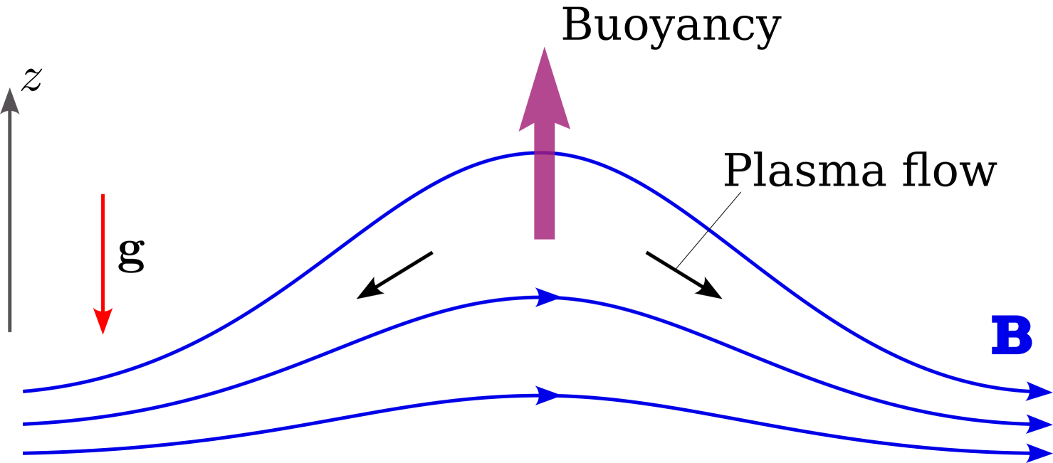
Figure 12: Schematic of the Parker instability.

Appendix A Numerical solution of Equation (17) for the case $\displaystyle r_{\mathrm{{out}}}>{r_{0}}$

It is instructive to directly solve Eq. (2.4) in the case when the outer boundary of the flow lies beyond the point $\displaystyle r_{0}$, where the potential $\displaystyle U(r_{0})=0$. In dimensionless variables $\displaystyle x=r/r_{0}$ and $\displaystyle\tilde{E}=-k_{z}^{2}r_{0}^{2}$, Eq. (2.4) reads:

$$\frac{{\rm d}^{2}\Psi}{{\rm d}x^{2}}+\left\{\tilde{E}-\tilde{U}\right\}\Psi=0\,,\quad\tilde{U}=\frac{3}{4}\frac{1}{x^{2}}-\frac{3}{4}\frac{1}{x^{3}}\,.$$ (79)

The amplitude of the function $\displaystyle\Psi$ is arbitrary, and we choose $\displaystyle|\Psi(x_{1})|=1$. Conditions at the boundaries of the flow are imposed according to (30).

We can simplify the numerical solution by imposing a condition not at the outer boundary point $\displaystyle x_{\mathrm{out}}>1$, but at the turning point $\displaystyle x_{1}<1$. At the turning point $\displaystyle x_{1}$, the condition $\displaystyle\Psi^{\prime\prime}(x_{1})=0$ is automatically satisfied due to the nature of the turning point, where $\displaystyle\tilde{U}(x_{1})=\tilde{E}$. Therefore, as a boundary condition at the turning point, we should take the value of the first derivative $\displaystyle\Psi^{\prime}(x_{1})$. It can be easily found by noticing that for small $\displaystyle\xi=x-x_{1}\ll 1$, Eq. (79) reduces to the Airy equation

$$\Psi^{\prime\prime}(z)+z\Psi=0\,,$$ (80)

where

$$z=\left(\frac{3}{2}\frac{1}{x_{1}^{3}}-\frac{9}{4}\frac{1}{x_{1}^{4}}\right)^{1/3}\xi\,.$$ (81)

The general solution of Eq. (80) is

$$\mathrm{Ai}(z)=\frac{\sqrt{z}}{3}\left[J_{1/3}(\frac{2}{3}(-z)^{3/2})+J_{-1/3}(\frac{2}{3}(-z)^{3/2})\right]\,.$$ (82)

It should be clear that if the outer boundary $\displaystyle x_{\mathrm{out}}\to\infty$, then $\displaystyle\Psi\to 0$, and the constant in the general solution $\displaystyle C_{2}$ must be equal to zero. For a finite $\displaystyle x_{\mathrm{out}}$, the constant $\displaystyle C_{2}$ is non-zero, and the value of the first derivative $\displaystyle\Psi^{\prime}(x_{1})$ should be determined from the conditions at the outer and inner boundaries (30). Below, we present solutions for the case of $\displaystyle x_{\mathrm{out}}\gg 1$ with the constant $\displaystyle C_{2}=0$.

At the point $\displaystyle x_{1}$, where $\displaystyle\xi=z=0$, the first derivative reads:

$$\left.\frac{{\rm d}\Psi}{{\rm d}x}\right|_{x_{1}}=\left.\frac{{\rm d}\Psi}{{\rm d}z}\frac{{\rm d}z}{{\rm d}x}\right|_{x_{1}}=C_{1}\,\mathrm{Ai}^{\prime}(0)\,\left[\frac{3}{2}\frac{1}{x_{1}^{3}}-\frac{9}{4}\frac{1}{x_{1}^{4}}\right]^{1/3}\,,$$ (83)

where $\displaystyle\mathrm{Ai}^{\prime}(0)=0.25882\ldots$

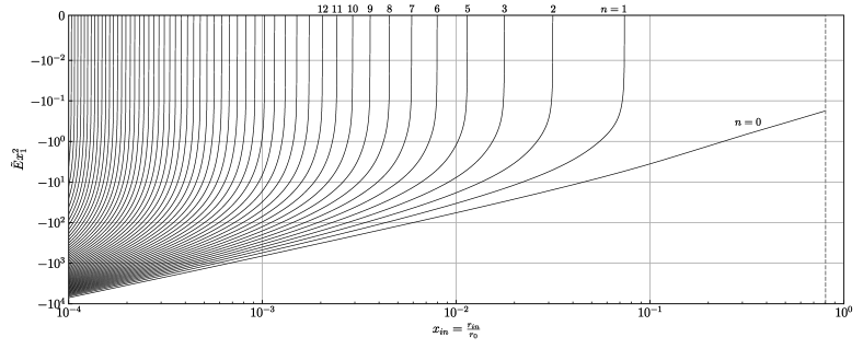
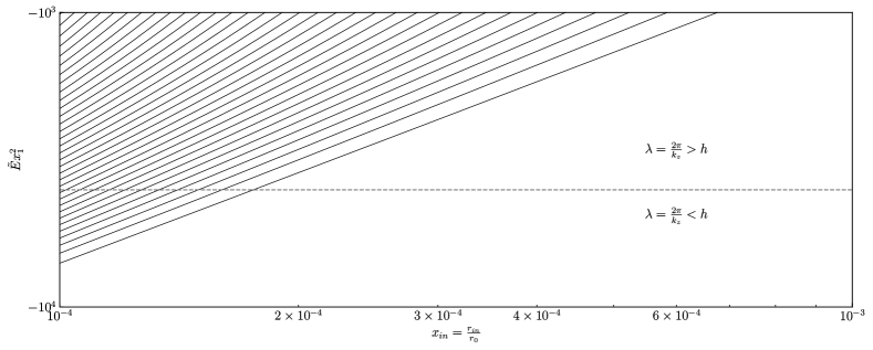
Figure 14: (a) Discrete ”energy levels” $\displaystyle\tilde{E}=-(k_{z}r_{0})^{2}$ of Eq. (79) for different inner boundaries $\displaystyle x_{\mathrm{in}}$. As $\displaystyle x_{\mathrm{in}}$ decreases, the number of discrete ”energy levels” $\displaystyle n=0,1,2,3\ldots$ of the function $\displaystyle\Psi$ increases. Deep ”energy levels” with $\displaystyle-\tilde{E}x_{1}^{2}>4\times 10^{3}$ appear when $\displaystyle\log x_{\mathrm{in}}<-3.756$. There exists a maximum value of $\displaystyle x_{\mathrm{in}}\approx 0.8116$ with $\displaystyle\tilde{E}_{0}\approx-0.2644$ for the eigenmode with $\displaystyle n=0$. Other modes $\displaystyle n=1,2,\ldots$ can have $\displaystyle\tilde{E}=0$ at certain values of $\displaystyle x_{\mathrm{in}}$. (b) The region of ”deep levels” and the boundary $\displaystyle\lambda=2\pi/k_{z}=h=0.1\,r$  for thin accretion discs (see section 2.6).

Integration of Eq. (79) with the boundary conditions (30) $\displaystyle\Psi^{\prime}|_{x_{\mathrm{in}}}+{\Psi}/({2x_{\mathrm{in}}})=0$ and Eq. (83) for various values of $\displaystyle x_{\mathrm{in}}$ yields a family of solutions with discrete (non-equidistant) ”energy levels” $\displaystyle\tilde{E}_{n}$ (or equivalently, according to Eq. (27), with discrete turning points $\displaystyle x_{1}$) corresponding to the integer number $\displaystyle n=0,1,2,3,\ldots$ of the zeros of the function $\displaystyle\Psi$. It should be noted that for a given $\displaystyle x_{\mathrm{in}}$, there exists a different number of possible energy levels, and there is a maximum value $\displaystyle(x_{\mathrm{in}})_{\mathrm{max}}\approx 0.8116$ that allows the existence of a single level for $\displaystyle n=0$. The solutions, normalized to the maximum value of the function $\displaystyle\Psi$, are shown in Fig. 13. The discrete ”energy levels” $\displaystyle\tilde{E}=-(k_{z}r_{0})^{2}$ of Eq. (79) for different inner boundaries $\displaystyle x_{\mathrm{in}}$ are shown in Fig. 14. The values of the energy $\displaystyle\tilde{E}$ for different levels at fixed $\displaystyle x_{\mathrm{in}}$ under various boundary conditions on the function $\displaystyle\Psi$ are presented in Table 1. It is evident that the type of boundary conditions has a weak influence on the energy values of the ”lower” levels in deep potential wells for $\displaystyle x_{\mathrm{in}}\ll 1$.

Table 1: Examples of energy levels $\displaystyle\tilde{E}$ of Eq. (79) for $\displaystyle x_{\mathrm{in}}=0.1,0.01,0.001$ and different conditions at the inner boundary $\displaystyle x_{\mathrm{in}}$.

$\displaystyle n_{\tilde{E}}$	$\displaystyle\left.\left(\Psi^{\prime}+{\Psi}/({2x})\right)\right|_{x_{\mathrm{in}}}=0$	$\displaystyle\Psi^{\prime}|_{x_{\mathrm{in}}}=0$	$\displaystyle\Psi|_{x_{\mathrm{in}}}=0$
$\displaystyle x_{\mathrm{in}}=0.1$
0	$\displaystyle-118.86$	$\displaystyle-86.44$	–
$\displaystyle x_{\mathrm{in}}=0.01$
4	$\displaystyle-8.168$	$\displaystyle-7.096$	–
3	$\displaystyle-9.799\times 10^{2}$	$\displaystyle-9.250\times 10^{2}$	$\displaystyle-1.229\times 10^{2}$
2	$\displaystyle-1.189\times 10^{4}$	$\displaystyle-1.145\times 10^{4}$	$\displaystyle-3.483\times 10^{3}$
1	$\displaystyle-7.057\times 10^{4}$	$\displaystyle-6.846\times 10^{4}$	$\displaystyle-2.808\times 10^{4}$
0	$\displaystyle-3.423\times 10^{5}$	$\displaystyle-3.288\times 10^{5}$	$\displaystyle-1.408\times 10^{5}$
$\displaystyle x_{\mathrm{in}}=0.001$
16	$\displaystyle-2.666$	$\displaystyle-2.525$	–
15	$\displaystyle-6.314\times 10^{2}$	$\displaystyle-6.190\times 10^{2}$	$\displaystyle-7.436\times 10^{1}$
14	$\displaystyle-8.869\times 10^{3}$	$\displaystyle-8.762\times 10^{3}$	$\displaystyle-2.668\times 10^{3}$
13	$\displaystyle-5.308\times 10^{4}$	$\displaystyle-5.260\times 10^{4}$	$\displaystyle-2.266\times 10^{4}$
12	$\displaystyle-2.078\times 10^{5}$	$\displaystyle-2.063\times 10^{5}$	$\displaystyle-1.071\times 10^{5}$
11	$\displaystyle-6.287\times 10^{5}$	$\displaystyle-6.250\times 10^{5}$	$\displaystyle-3.650\times 10^{5}$
10	$\displaystyle-1.598\times 10^{6}$	$\displaystyle-1.590\times 10^{6}$	$\displaystyle-1.007\times 10^{6}$
9	$\displaystyle-3.585\times 10^{6}$	$\displaystyle-3.569\times 10^{6}$	$\displaystyle-2.397\times 10^{6}$
8	$\displaystyle-7.319\times 10^{6}$	$\displaystyle-7.290\times 10^{6}$	$\displaystyle-5.121\times 10^{6}$
7	$\displaystyle-1.390\times 10^{7}$	$\displaystyle-1.385\times 10^{7}$	$\displaystyle-1.007\times 10^{7}$
6	$\displaystyle-2.495\times 10^{7}$	$\displaystyle-2.486\times 10^{7}$	$\displaystyle-1.857\times 10^{7}$
5	$\displaystyle-4.284\times 10^{7}$	$\displaystyle-4.271\times 10^{7}$	$\displaystyle-3.258\times 10^{7}$
4	$\displaystyle-7.115\times 10^{7}$	$\displaystyle-7.094\times 10^{7}$	$\displaystyle-5.496\times 10^{7}$
3	$\displaystyle-1.155\times 10^{8}$	$\displaystyle-1.151\times 10^{8}$	$\displaystyle-9.011\times 10^{7}$
2	$\displaystyle-1.854\times 10^{8}$	$\displaystyle-1.848\times 10^{8}$	$\displaystyle-1.451\times 10^{8}$
1	$\displaystyle-3.005\times 10^{8}$	$\displaystyle-2.994\times 10^{8}$	$\displaystyle-2.328\times 10^{8}$
0	$\displaystyle-5.263\times 10^{8}$	$\displaystyle-5.227\times 10^{8}$	$\displaystyle-3.828\times 10^{8}$

Table 2: Values of the dimensionless inner flow boundary for zero energy $\displaystyle x_{\mathrm{in}}|_{\tilde{E}=0}$ under different choices of boundary conditions. The value of $\displaystyle x_{\mathrm{in}}|_{\tilde{E}=0}$ in the WKB approximation is given by (87) and (88). It is noteworthy that under the third-type boundary condition (free boundary), the zero energy level is reached at a finite value of $\displaystyle\tilde{E}\approx-0.2644$ corresponding to $\displaystyle x_{\mathrm{in}}\approx 0.8116$. Refer to Fig. 14 for further details.

$\displaystyle n_{\tilde{E}}$	$\displaystyle\left.\left(\Psi^{\prime}+{\Psi}/({2x})\right)\right|_{x_{\mathrm{in}}}=0$	$\displaystyle\Psi^{\prime}|_{x_{\mathrm{in}}}=0$	$\displaystyle\Psi|_{x_{\mathrm{in}}}=0$
…	…	…	…
16	$\displaystyle 1.02496\times 10^{-3}$	$\displaystyle 1.02426\times 10^{-3}$	—
15	$\displaystyle 1.15546\times 10^{-3}$	$\displaystyle 1.15457\times 10^{-3}$	$\displaystyle 1.08531\times 10^{-3}$
14	$\displaystyle 1.31260\times 10^{-3}$	$\displaystyle 1.31145\times 10^{-3}$	$\displaystyle 1.22775\times 10^{-3}$
13	$\displaystyle 1.50417\times 10^{-3}$	$\displaystyle 1.50266\times 10^{-3}$	$\displaystyle 1.40021\times 10^{-3}$
12	$\displaystyle 1.74105\times 10^{-3}$	$\displaystyle 1.73903\times 10^{-3}$	$\displaystyle 1.61176\times 10^{-3}$
11	$\displaystyle 2.03875\times 10^{-3}$	$\displaystyle 2.03598\times 10^{-3}$	$\displaystyle 1.87519\times 10^{-3}$
10	$\displaystyle 2.42010\times 10^{-3}$	$\displaystyle 2.41620\times 10^{-3}$	$\displaystyle 2.20897\times 10^{-3}$
9	$\displaystyle 2.91976\times 10^{-3}$	$\displaystyle 2.91407\times 10^{-3}$	$\displaystyle 2.64061\times 10^{-3}$
8	$\displaystyle 3.59244\times 10^{-3}$	$\displaystyle 3.58384\times 10^{-3}$	$\displaystyle 3.21255\times 10^{-3}$
7	$\displaystyle 4.52880\times 10^{-3}$	$\displaystyle 4.51513\times 10^{-3}$	$\displaystyle 3.99300\times 10^{-3}$
6	$\displaystyle 5.88807\times 10^{-3}$	$\displaystyle 5.86497\times 10^{-3}$	$\displaystyle 5.09744\times 10^{-3}$
5	$\displaystyle 7.97202\times 10^{-3}$	$\displaystyle 7.92969\times 10^{-3}$	$\displaystyle 6.73423\times 10^{-3}$
4	$\displaystyle 1.14131\times 10^{-2}$	$\displaystyle 1.13263\times 10^{-2}$	$\displaystyle 9.31161\times 10^{-3}$
3	$\displaystyle 1.77392\times 10^{-2}$	$\displaystyle 1.75298\times 10^{-2}$	$\displaystyle 1.37231\times 10^{-2}$
2	$\displaystyle 3.15576\times 10^{-2}$	$\displaystyle 3.08961\times 10^{-2}$	$\displaystyle 2.22593\times 10^{-2}$
1	$\displaystyle 7.39693\times 10^{-2}$	$\displaystyle 7.03546\times 10^{-2}$	$\displaystyle 4.24509\times 10^{-2}$
0	$\displaystyle 0.8116|_{\tilde{E}=-0.2644}$	$\displaystyle 5.87626\times 10^{-1}$	$\displaystyle 1.14244\times 10^{-1}$

It should be noted that Eq. (79) can be solved using the quasi-classical (WKB) approximation, employing the Bohr-Sommerfeld condition for discrete energy levels $\displaystyle E=-k_{z}^{2}<0$ with index $\displaystyle n=0,1,2,\ldots$ in the potential $\displaystyle U$ for rigid boundaries (Landau and Lifshitz 1977, Flugge 1971):

$$\int\limits_{r_{\mathrm{in}}}^{r_{1}}\sqrt{E-U}\,dr=\piup\left(n+\frac{3}{4}\right)\,;\quad n=0,1,2,\ldots$$ (84)

Here, $\displaystyle r_{1}$ is the turning point in the potential $\displaystyle U$, which can be found from Eq. (26). The existence of stationary levels with negative energy and $\displaystyle\omega^{2}<0$ indicates the instability of the flow. A similar equation, but with a constant slightly different from 3/4, can be obtained for a free boundary. However, for large $\displaystyle n\gg 1$, all three boundary conditions ($\displaystyle\Psi|_{x_{\mathrm{in}}}=0$, $\displaystyle\Psi^{\prime}|_{x_{\mathrm{in}}}=0$, $\displaystyle(\Psi^{\prime}+{\Psi}/(2{x}))|_{x_{\mathrm{in}}}=0$) yield the same result.

In dimensionless units with the energy $\displaystyle\tilde{E}=-k_{z}^{2}r_{0}^{2}$ and potential $\displaystyle\tilde{U}$, Eq. (84) takes the form

$$\int\limits_{x_{\mathrm{in}}}^{x_{1}}\sqrt{\tilde{E}-\frac{3}{4x^{2}}+\frac{3}{4x^{3}}}\,{\rm d}x=\piup\,\left(n+\frac{3}{4}\right)\,.$$ (85)

In the case of a large perturbation wavelength, $\displaystyle\tilde{E}=-k_{z}^{2}r_{0}^{2}\ll 1$. At low energies $\displaystyle\tilde{E}\approx 0$, the turning point tends to the zero of the potential, $\displaystyle r_{1}\to r_{0}$, and the integral in Eq. (85) is

$$\int\limits_{x_{\mathrm{in}}}^{1}\sqrt{-\frac{3}{4x^{2}}+\frac{3}{4x^{3}}}\,{\rm d}x=\piup\,\left(n+\frac{3}{4}\right)\,.$$ (86)

This integral is taken as follows:

$$\sqrt{3}\left[\sqrt{\frac{1}{x_{\mathrm{in}}}-1}+\arcsin{\sqrt{x_{\mathrm{in}}}}-\frac{\piup}{2}\right]=\piup\left(n+\frac{3}{4}\right)$$ (87)

(compare with equation (2.24) for the case of isomoment rotation with circular velocity $\displaystyle v_{\phi}\propto 1/r$ in the original paper by Velikhov (1959); here, we consider the Keplerian case with $\displaystyle v_{\phi}\propto 1/\sqrt{r}$). From Eq. (87), we find the first $\displaystyle x_{\mathrm{in}}$ for $\displaystyle n=0$: $\displaystyle x_{\mathrm{in}}\approx 0.575$. The exact value, which we obtained numerically (see Fig. 14), is $\displaystyle(x_{\mathrm{in}})_{\mathrm{max}}\approx 0.8116$. Furthermore, under the given third-type boundary conditions, the energy value for the mode with $\displaystyle n=0$ is approximately $\displaystyle\tilde{E}[(x_{\mathrm{in}})_{\mathrm{max}}]\approx-0.2644$, and for modes $\displaystyle n=1,2,\ldots$, there always exists a discrete value of $\displaystyle x_{\mathrm{in}}$ for which $\displaystyle\tilde{E}=0$. For first and second-type boundary conditions, $\displaystyle E[(x_{\mathrm{in}})_{\mathrm{max}}]=0$ (see Table 1 and 2 for different conditions at the inner boundary). For $\displaystyle x_{\mathrm{in}}>(x_{\mathrm{in}})_{\mathrm{max}}$, the potential well becomes so shallow that there are no stationary ”energy levels”. It is worth noting that the accuracy of the WKB approximation increases for large $\displaystyle n$. In our case, for $\displaystyle x_{\mathrm{in}}=r_{\mathrm{in}}/r_{0}\ll 1$, the discrete values of $\displaystyle x_{\mathrm{in}}$ are given by:

$$x_{\mathrm{in}}=\frac{1}{\left[\left({\piup}/\sqrt{3}\right)\left(n+{3}/{4}\right)+{\piup}/{2}\right]^{2}+1}\,.$$ (88)

In principle, the integral in Eq. (85) can be numerically computed for any value of $\displaystyle\tilde{E}$ to find the discrete energy levels $\displaystyle\tilde{E}_{n}$ at fixed $\displaystyle x_{\mathrm{in}}$ (especially for large $\displaystyle|\tilde{E}|$ corresponding to thin accretion disks, as mentioned above) for any $\displaystyle n$. However, precise numerical solutions of Eq. (79) have already been obtained.

It is worth noting that, if we disregard the term $\displaystyle{3}/\left({4}{x^{2}}\right)$ in Eq. (85), it can be solved analytically (see Latter et al. 2015). The WKB solution is found to be in excellent agreement with the numerical results.

Appendix B Case $\displaystyle r_{\mathrm{out}}<r_{0}$

If the outer boundary of the flow, denoted as $\displaystyle r_{\mathrm{out}}$, is smaller than $\displaystyle r_{0}$ (the point at which the potential becomes zero, $\displaystyle U(r_{0})=0$, see Eq. (23)), then the problem of finding the stationary energy levels of Eq. (79) needs to be numerically solved with the boundary conditions given by (30). In the case of a narrow flow (when the outer radius is close to the inner radius), the problem has an analytical solution. A similar problem, with a different rotational law and zero boundary conditions for magnetic field perturbations ($\displaystyle b_{r}=0$, corresponding to the condition $\displaystyle\Psi=0$), was solved by Velikhov (1959).

Let us introduce the following notations:

$$\bar{r}\equiv r_{\mathrm{in}}+\frac{r_{\mathrm{out}}-r_{\mathrm{in}}}{2},\qquad\Delta\equiv r_{\mathrm{out}}-r_{\mathrm{in}}\ll\bar{r}\,.$$ (89)

When the parameter $\displaystyle\bar{r}$ is fixed, Eq. (79) transforms into a Sturm-Liouville problem with homogeneous boundary conditions of the third kind on the interval $\displaystyle x\in[a,b]$:

$$\begin{cases}&\Psi^{\prime\prime}+\lambda\Psi=0\,,\\ &\Psi^{\prime}|_{a}+\frac{\Psi}{2a}=0\,,\\ &\Psi^{\prime}|_{b}+\frac{\Psi}{2b}=0\,,\end{cases}$$ (90)

where

$$\lambda=-k_{z}^{2}-\frac{3}{4}\frac{1}{\bar{r}^{2}}+\frac{GM}{\bar{r}^{3}}\frac{{\omega^{2}}/{k_{z}^{2}}+3\,c_{A}^{2}}{\left(c_{A}^{2}-{\omega^{2}}/{k_{z}^{2}}\right)^{2}}\,.$$ (91)

This problem admits the existence of only positive nontrivial eigenvalues $\displaystyle\lambda_{n}>0$, corresponding to oscillating eigenfunctions $\displaystyle\Psi_{n}$. Then, the general solution of Eq. (90) is given by

$$\Psi=C_{1}\sin(\sqrt{\lambda}x)+C_{2}\cos(\sqrt{\lambda}x)\,.$$ (92)

The constants $\displaystyle C_{1}$ and $\displaystyle C_{2}$ are determined by the boundary conditions. By excluding the trivial solution $\displaystyle\lambda=0$, we obtain the following system of equations:

$$\begin{cases}&C_{1}\left(1+\frac{1}{2\sqrt{\lambda}a}\tan(\sqrt{\lambda}a)\right)+C_{2}\left(\frac{1}{2\sqrt{\lambda}a}-\tan(\sqrt{\lambda}a)\right)=0\,,\\ &C_{1}\left(1+\frac{1}{2\sqrt{\lambda}b}\tan(\sqrt{\lambda}b)\right)+C_{2}\left(\frac{1}{2\sqrt{\lambda}b}-\tan(\sqrt{\lambda}b)\right)=0\,.\end{cases}$$ (93)

System (93) has a nontrivial solution when the determinant is equal to zero. This leads to a transcendental equation for finding the eigenvalues $\displaystyle\lambda$:

$$\displaystyle\left[\frac{1}{2\sqrt{\lambda}b}-\frac{1}{2\sqrt{\lambda}a}\right]\,\left(1+\tan(\sqrt{\lambda}a)\,\tan(\sqrt{\lambda}b)\right)+$$

$$\displaystyle\left[1+\frac{1}{4\lambda ab}\right]\,\left(\tan(\sqrt{\lambda}a)-\tan(\sqrt{\lambda}b)\right)=0\,.$$ (94)

Equation (B) has two families of solutions:

$$\begin{cases}&1+\tan(\sqrt{\lambda}a)\tan(\sqrt{\lambda}b)=0\\ &-\tan(\sqrt{\lambda}(b-a))=\frac{\sqrt{\lambda}(b-a)}{1+4\lambda ab}\end{cases}$$ (95)

The first family of solutions to Eq. (B) is given by

$$\cos\left(\sqrt{\lambda}\,[a-b]\right)=0\,.$$ (96)

From this, we obtain the set of eigenvalues

$$\lambda_{n}=\frac{\left({\pi}/{2}+n\pi\right)^{2}}{\Delta^{2}}\,,\qquad n=0,1,2,3,\ldots$$ (97)

For small values of $\displaystyle n=1,2,3,...$, the second family of solutions (95) can be found numerically. However, for large argument values, it quickly converges to $\displaystyle\lambda_{n}\approx\pi^{2}n^{2}/\Delta^{2}$ for $\displaystyle n\gg 1$. Therefore, for large $\displaystyle n$, both solutions can be combined into a single expression: $\displaystyle\lambda_{n}\approx(\pi^{2}/4)(1+n)^{2}/\Delta^{2}$. It should be noted that under first-kind homogeneous boundary conditions $\displaystyle\Psi|_{a,b}=0$ or second-kind homogeneous boundary conditions $\displaystyle\Psi^{\prime}|_{a,b}=0$, the following solutions are obtained:

$$\displaystyle\sin\sqrt{\lambda}(b-a)=0\quad\to\quad\lambda_{n}=\frac{\pi^{2}n^{2}}{\Delta^{2}}\,,$$

$$\displaystyle\sin\sqrt{\lambda}(a+b)=0\quad\to\quad\lambda_{n}=\frac{\pi^{2}n^{2}}{(a+b)^{2}}\,,$$

$$\displaystyle n=1,2,3,\ldots$$ (98)

From (97), we obtain a set of equations for each eigenvalue $\displaystyle\lambda_{n}$:

$$\displaystyle-k_{z}^{2}-\frac{3}{4}\frac{1}{\bar{r}^{2}}+\frac{GM}{\bar{r}^{3}}\frac{{\omega^{2}}/{k_{z}^{2}}+3c_{A}^{2}}{\left(c_{A}^{2}-{\omega^{2}}/{k_{z}^{2}}\right)^{2}}=\lambda_{n}\approx\frac{\pi^{2}(n+1)^{2}}{4\Delta^{2}}\,,$$

$$\displaystyle n=0,1,2,3,\ldots$$ (99)

Hence, we obtain the dispersion equations in the following form:

$$\displaystyle\frac{\omega^{2}}{c_{A}^{2}\,k_{z}^{2}}=\left(1+\frac{K}{2}\right)\,\left[1\pm\sqrt{1+\frac{4(3K-1)}{(K+2)^{2}}}\,\right]\,,$$

$$\displaystyle K\approx\frac{v_{\phi}^{2}(\bar{r})}{c_{a}^{2}}\frac{1}{{\pi^{2}}/{4}\,(n+1)^{2}\left({\bar{r}}/{\Delta}\right)^{2}+k_{z}^{2}\bar{r}^{2}+{3}/{4}}\,.$$ (100)

For unstable modes with $\displaystyle\omega^{2}<0$, in the dispersion equation (B), we keep the minus sign before the square root and require $\displaystyle K>1/3$, which leads to the appearance of a critical magnetic field for the MRI mode:

$$c_{A}^{2}<(c_{A}^{2})_{cr}\approx\frac{4v_{\phi}^{2}(\bar{r})}{({1}/{3})\pi^{2}(n+1)^{2}\left({\bar{r}}/{\Delta}\right)^{2}+\frac{4}{3}k_{z}^{2}\bar{r}^{2}+1}\,.$$ (101)

It should be noted that for the first and second kind boundary conditions, the critical field values are given by

$$\begin{cases}&(c_{A}^{2})_{cr}=\frac{4v_{\phi}^{2}(\bar{r})}{({4}/{3})\pi^{2}n^{2}\left({\bar{r}}/{\Delta}\right)^{2}+({4}/{3})k_{z}^{2}\bar{r}^{2}+1}\,,\quad\Psi|_{a,b}=0\\ &(c_{A}^{2})_{cr}=\frac{4v_{\phi}^{2}(\bar{r})}{({1}{3})\pi^{2}n^{2}+({4}/{3})k_{z}^{2}\bar{r}^{2}+1}\,,\quad\Psi^{\prime}|_{a,b}=0\end{cases}$$ (102)

The similarity of results between the first and third kind boundary conditions is notable.

Lastly, it is noteworthy that for the case of $\displaystyle r_{\mathrm{out}}<r_{0}$ (when the potential has the same sign over the entire interval $\displaystyle[r_{\mathrm{in}},r_{\mathrm{out}}]$), the asymptotic behavior of eigenvalues is given by $\displaystyle\lambda_{n}\sim\pi^{2}n^{2}/(r_{\mathrm{out}}-r_{\mathrm{in}})^{2}$ for large $\displaystyle n\gg 1$, which follows from the general theorems of the Sturm-Liouville problem for any continuous potential with a consistent sign (see, for example, Levitan and Sargsjan 2012).

References

- (1)
- Acheson (1990) Acheson, D.: 1990, Elementary Fluid Dynamics, Oxford, Clarendon Press.
- Bai and Stone (2013) Bai, X.-N. and Stone, J. M.: 2013, Wind-driven Accretion in Protoplanetary Disks. I. Suppression of the Magnetorotational Instability and Launching of the Magnetocentrifugal Wind, ApJ 769(1), 76.
- Balbus and Hawley (1991) Balbus, S. A. and Hawley, J. F.: 1991, A powerful local shear instability in weakly magnetized disks. I - Linear analysis. II - Nonlinear evolution, ApJ 376, 214–233.
- Balbus and Hawley (1998) Balbus, S. A. and Hawley, J. F.: 1998, Instability, turbulence, and enhanced transport in accretion disks, Reviews of Modern Physics 70, 1–53.
- Bisnovatyi-Kogan and Lovelace (2001) Bisnovatyi-Kogan, G. S. and Lovelace, R. V. E.: 2001, Advective accretion disks and related problems including magnetic fields, New Astron. 45(11-12), 663–742.
- Boneva et al. (2021) Boneva, D. V., Mikhailov, E. A., Pashentseva, M. V. and Sokoloff, D. D.: 2021, Magnetic fields in the accretion disks for various inner boundary conditions, A&A 652, A38.
- Chandrasekhar (1960) Chandrasekhar, S.: 1960, The Stability of Non-Dissipative Couette Flow in Hydromagnetics, Proceedings of the National Academy of Science 46, 253–257.
- Curry and Pudritz (1996) Curry, C. and Pudritz, R. E.: 1996, On the global stability of magnetized accretion discs - III. Non-axisymmetric modes, MNRAS 281(1), 119–136.
- Curry et al. (1994) Curry, C., Pudritz, R. E. and Sutherland, P. G.: 1994, On the Global Stability of Magnetized Accretion Disks. I. Axisymmetric Modes, ApJ 434, 206.
- Dubrulle and Knobloch (1993) Dubrulle, B. and Knobloch, E.: 1993, On instabilities in magnetized accretion disks, A&A 274, 667.
- Flugge (1971) Flugge, S.: 1971, Practical Quantum Mechanics, 2 volumes, Springer-Verlag.
- Gammie and Balbus (1994) Gammie, C. F. and Balbus, S. A.: 1994, Quasi-Global Linear Analysis of a Magnetized Disc, MNRAS 270, 138.
- Hawley et al. (1995) Hawley, J. F., Gammie, C. F. and Balbus, S. A.: 1995, Local Three-dimensional Magnetohydrodynamic Simulations of Accretion Disks, ApJ 440, 742.
- Hawley et al. (2013) Hawley, J. F., Richers, S. A., Guan, X. and Krolik, J. H.: 2013, Testing Convergence for Global Accretion Disks, ApJ 772, 102.
- Kato et al. (1998) Kato, S., Fukue, J. and Mineshige, S.: 1998, Black-hole accretion disks, Kyoty University Press.
- Knobloch (1992) Knobloch, E.: 1992, On the stability of magnetized accretion discs, MNRAS 255, 25P–28P.
- Kumar et al. (1994) Kumar, S., Coleman, C. S. and Kley, W.: 1994, The Axisymmetric Instability in Weakly Magnetized Accretion Discs, MNRAS 266, 379.
- Landau and Lifshitz (1959) Landau, L. D. and Lifshitz, E. M.: 1959, Fluid mechanics, Vol. 6 of Course of Theoretical Physics, Pergamon Press, Oxford.
- Landau and Lifshitz (1977) Landau, L. and Lifshitz, E.: 1977, Quantum Mechanics. Non-relativistic theory, Pergamon Press Ltd., London.
- Latter et al. (2015) Latter, H. N., Fromang, S. and Faure, J.: 2015, Local and global aspects of the linear MRI in accretion discs, MNRAS 453(3), 3257–3268.
-
Levitan and Sargsjan (2012)
Levitan, B. and Sargsjan, I.: 2012, Sturm—Liouville and Dirac
Operators, Mathematics and its Applications, Springer Netherlands.
https://books.google.de/books?id=I5HpCAAAQBAJ - Lipunova et al. (2018) Lipunova, G., Malanchev, K. and Shakura, N.: 2018, The Standard Model of Disc Accretion, in N. Shakura (ed.), Astrophysics and Space Science Library, Vol. 454 of Astrophysics and Space Science Library, p. 1.
- Lord Rayleigh (1916) Lord Rayleigh: 1916, , Proc. R. Soc. A 93, 143.
- Papaloizou and Szuszkiewicz (1992) Papaloizou, J. and Szuszkiewicz, E.: 1992, The stability of a differentially rotating disc with a poloidal magnetic field, Geophysical and Astrophysical Fluid Dynamics 66(1), 223–242.
- Parker (1966) Parker, E. N.: 1966, The Dynamical State of the Interstellar Gas and Field, ApJ 145, 811.
- Salmeron et al. (2007) Salmeron, R., Königl, A. and Wardle, M.: 2007, Angular momentum transport in protostellar discs, MNRAS 375(1), 177–183.
- Shakura and Lipunova (2018) Shakura, N. I. and Lipunova, G. V.: 2018, Logarithmic potential for the gravitational field of Schwarzschild black holes, MNRAS 480(3), 4273–4277.
- Shakura and Sunyaev (1973) Shakura, N. I. and Sunyaev, R. A.: 1973, Black holes in binary systems. Observational appearance., A&A 24, 337–355.
- Shakura and Postnov (2015a) Shakura, N. and Postnov, K.: 2015a, A viscous-convective instability in laminar Keplerian thindiscs - II. Anelastic approximation, MNRAS 451(4), 3995–4004.
- Shakura and Postnov (2015b) Shakura, N. and Postnov, K.: 2015b, On properties of Velikhov-Chandrasekhar MRI in ideal and non-ideal plasma, MNRAS 448(4), 3697–3706.
- Shakura and Postnov (2018) Shakura, N. and Postnov, K.: 2018, On the Properties of Velikhov-Chandrasekhar MRI in Ideal and Non-ideal Plasmas, in N. Shakura (ed.), Astrophysics and Space Science Library, Vol. 454 of Astrophysics and Space Science Library, p. 393.
- Somov et al. (2003) Somov, B. V., Oreshina, A. V., Oreshina, I. V. and Shakura, N. I.: 2003, Flares in accretion disk coronae, Advances in Space Research 32(6), 1087–1096.
- Sorathia et al. (2012) Sorathia, K. A., Reynolds, C. S., Stone, J. M. and Beckwith, K.: 2012, Global Simulations of Accretion Disks. I. Convergence and Comparisons with Local Models, ApJ 749, 189.
- Velikhov (1959) Velikhov, E. P.: 1959, , Sov. Phys. JETP 36, 1398.
- Zou et al. (2020) Zou, R., Labarbe, J., Kirillov, O. N. and Fukumoto, Y.: 2020, Analysis of azimuthal magnetorotational instability of rotating magnetohydrodynamic flows and Tayler instability via an extended Hain-Lüst equation, Phys. Rev. E 101(1), 013201.