Modelling of discrete extremes through extended versions of discrete generalized Pareto distribution

Abstract

The statistical modelling of integer-valued extremes such as large avalanche counts has received less attention than their continuous counterparts in the extreme value theory (EVT) literature. One approach to moving from continuous to discrete extremes is to model threshold exceedances of integer random variables by the discrete version of the generalized Pareto distribution. Still, the optimal threshold selection that defines exceedances remains a problematic issue. Moreover, within a regression framework, the treatment of the many data points (those below the chosen threshold) is either ignored or decoupled from extremes. Considering these issues, we extend the idea of using a smooth transition between the two tails (lower and upper) to force large and small discrete extreme values to comply with EVT. In the case of zero inflation, we also develop models with an additional parameter. To incorporate covariates, we extend the Generalized Additive Models (GAM) framework to discrete extreme responses. In the GAM forms, the parameters of our proposed models are quantified as a function of covariates. The maximum likelihood estimation procedure is implemented for estimation purposes. With the advantage of bypassing the threshold selection step, our findings indicate that the proposed models are more flexible and robust than competing models (i.e. discrete generalized Pareto distribution and Poisson distribution).

Keywords: Extreme value theory, Discrete extended generalized Pareto distribution, Zero-inflated models, Generalized additive models.

1 Introduction

Extreme Value Theory (EVT) originating from the innovative work of Fisher and Tippett (1928) offers a facility of stochastic modeling related to very high and very low frequency events (e.g., extreme temperature, heavy rainfall intensities, heavy floods and extreme winds etc.). For example, from last three decades, Coles (2001), Beirlant et al. (2004) and de Hann and Ferreira (2006) discussed regularly adapted extreme value models to measure uncertainty for continuous extremes events. More precisely, the distribution of exceedances (i.e., the amount of data appear over a given high threshold) is often approximated by the so-called Generalized Pareto distribution (GPD) defined by its cumulative distribution function (CDF) as

$$F(x;\sigma,\xi)=\begin{cases}1-\left(1+\xi x/\sigma\right)_{+}^{-1/\xi}&\xi\neq 0\\ 1-\exp{(-{x}/{\sigma})}&\xi=0\end{cases}$$ (1)

where $(a)_{+}=\max(a,0)$, $\sigma>0$ and $-\infty<\xi<+\infty$ represent the scale and shape parameters of the distribution, respectively. The shape parameter $\xi$ defines tail behavior of the GP distribution. If $\xi<0$, the upper tail is bounded. If $\xi=0$, this tends to the case of an exponential distribution, where all moments are finite. If $\xi>0$, the upper tail is unbounded but higher moments ultimately become infinite. Three defined cases are labeled “short-tailed”, “light-tailed”, and “heavy-tailed”, respectively. These types of tail behaviour makes GPD more flexible to model excesses.

Optimal threshold selection in GPD application is remains an arguable and elusive task (see, e.g. Dupuis, 1999; Scarrott and MacDonald, 2012). Numerous studies (for instance, Embrechts et al., 1999; Choulakian and Stephens, 2001; Davison and Smith, 1990; Katz et al., 2002; Boutsikas and Koutras, 2002) have established how the GPD can be fitted to continuous extreme events. This is vindicated by Pickands’ theorem (Pickands, 1975) which states that, for most random variables, the distribution of the exceedances converges to a GPD as the threshold increases to the right endpoint. One of the major disadvantages of GPD is that it only models those observations which occurs over a certain high threshold. This imposes an artificial dichotomy in the data (i.e., observations are either below or above the threshold) and the question of finding the optimal threshold remains complex for practitioners. In the continuous extreme value setting, many authors have been attempted to model entire range of data without threshold selection. For example, Frigessi et al. (2002) proposed dynamically weighted mixture model by combining light-tailed density and heavy tailed density (i.e., GPD) through weight function. The dynamically weighted mixture approach can be valuable in unsupervised tail estimation, especially in heavy tailed situations and for small percentiles. Frigessi’s model has many advantages but it has a drawback. For instance, the model has six parameters and inference is not a straightforward task ( see Frigessi et al., 2002, for more details). Carreau and Bengio (2009) proposed a semiparametric model called ”hybrid Pareto” model that stitches a Gaussian distribution with a heavy tailed GPD. According to Carreau and Bengio (2009), the hybrid Pareto model offers efficient estimates of the tail of the distributions and converges faster in terms of log-likelihood than existing GPD. They used hybrid Pareto models in regression context for statistical modeling of rainfall-runoff. MacDonald et al. (2011) combined a non-parametric kernel density estimator for the bulk of the distribution with a heavy-tailed GPD. One of drawback of these approaches is that it still needs to select the suitable threshold.

To keep a low number of parameters, avoid mixtures modeling and simplify inference, Naveau et al. (2016) proposed a general procedure to extend the GPD class. This construction is based on the integral transform idea to simulate GPD random draws, that is $F_{\sigma,\xi}^{-1}(U),$ where $U\sim\mathcal{U}(0,1)$ represents an uniformly distributed random variable on $(0,1)$ and $F_{\sigma,\xi}^{-1}$ denotes the inverse of the CDF (1). This leads to the class of random variables stochastically defined as

$$F_{\sigma,\xi}^{-1}\{G^{-1}(U)\},$$ (2)

where $G$ is a CDF on $[0,1]$ and $U\sim\mathcal{U}(0,1)$. The key problem is to find a class for $G$ which preserves the upper tail behavior with shape parameter $\xi$ and also controls the lower tail behavior. Naveau et al. (2016) defined restrictions for validity of $G$ families. For instance, the tail of $G$ denoted by $\bar{G}=1-G$ has to satisfy

$$\lim_{u\to 0}\frac{\bar{G}(1-u)}{u} = a,\mbox{ for some finite $a>0$ (upper tail behavior),}$$

$$\lim_{u\to 0}\frac{G(u)}{u^{\kappa}} = c,\mbox{ for some finite $c>0$ (lower tail behavior).}$$ (3)

Four examples for parametric family $G$ were studied in Naveau et al. (2016). By construction, this approach bypasses the elusive choice of a fixed and optimal threshold. Inference can be performed with classical methods such as maximum likelihood and probability weighted moments (see, e.g. Le Gall et al., 2022; Furrer and Naveau, 2007). Semi-parametric modeling based on this class has been studied by Tencaliec et al. (2019) and extensions to handle covariates have been proposed by Carrer and Gaetan (2022) and de Carvalho et al. (2022). Furthermore, Gamet and Jalbert (2022) modeled specific of tail estimation based on the same construction. Still, model (2) has to be yet tailored to handle discrete valued random variables.

The subsequent development deals with the discrete extreme models. A probability mass function (PMF) can be obtained by discretizing the CDF defined by (1) as

$$P(X=k)=F(k+1;\sigma,\xi)-F(k;\sigma,\xi),\hskip 28.45274ptk\in\mathbb{N}.$$ (4)

This is called a discrete GPD (DGPD). In existing literature, the DGPD have been used by Prieto et al. (2014) to model road accidents and Ranjbar et al. (2022) applied in regression context to model extremes of seasonal viruses and hospital congestion in Switzerland. Numerous features of discrete Pareto type distributions were studied in Krishna and Pundir (2009); Buddana and Kozubowski (2014); Kozubowski et al. (2015).

Similar to continuous GPD the DGPD is well approximated to discrete excesses over high threshold (Hitz et al., 2017). Again, an appropriate threshold selection procedure is required that can offer an optimal threshold for fitting DGPD. Also, the few questions arise in mind, the DGPD models the data above the threshold but how to model the observations below the threshold or how to model the entire range of count data having extreme observations.

One possibility is to use threshold spliced mixture representation for modeling the discrete observations. Again, the optimal threshold is needed for fitting threshold spliced mixture model. The detail is provided in ”Supplementary materials”. By keeping these arguments in mind, we want to develop the modeling framework which can be used to model the entire range of discrete extreme data without fixing threshold value. To introduce such modeling framework, we take advantage of the constructions given in Naveau et al. (2016). Thus, discrete extended versions of GPD (DEGPD) are proposed here by discretizing the CDF of continuous extended generalized Pareto distributions via equation (4). Discrete nature extreme events may contain a lot of zero values. For instance, the insurance complaints data or avalanches data may include many zero values. This type of data is generally referred to as zero-inflated (ZI), requiring specialized statistical methods for analysis. Therefore, we have introduced a zero-inflated version of DEGPD, ZIDEGPD. This model is useful for the data which has zero inflation and remaining observations rises from lower tail to mode of the distribution and then exponentially decay to the upper heavier tail.

Finally we aim to take into account covariate effects. This narrates to the work of Ranjbar et al. (2022), who model discrete exceedances with linear covariates effects by using generalized additive model (GAM) forms of DGPD in the same spirit as generalized additive models for location, scale and shape (Rigby and Stasinopoulos, 2005).

The paper is organized as follows. Section 2 presented the DEGPD and ZIDEGPD models along with simple sampling scheme. The GAM forms of DEGPD and ZIDEGPD are given in Section 3. To assess the performance of the proposed models, Section 4 provides the results of the conducted extensive simulation study. Section 5 discusses applications of DEGPD and ZIDEGPD to the number of upheld complaints data of insurance companies. Real application of GAM form models to avalanches data with environmental covariates are also given in the same section. Finally, Section 6 concludes with a summary of our results and a discussion of some future research directions.

2 Discrete extremes modeling

2.1 Discrete extended generalized Pareto distribution

We start by considering the CDF $G\left\{F\left(.;\sigma,\xi\right)\right\}$ of EGPD where $G$ meets the conditions (3). To model non-negative integer data, we discretize the CDF by

$$P(Y=k) = G\left\{F\left({k+1};\sigma,\xi\right)\right\}-G\left\{F\left({k};\sigma,\xi\right)\right\},\qquad k\in\mathbb{N}$$ (5)

The distribution defined by (5) will be called discrete extended generalized Pareto distribution (DEGPD). The explicit formula of CDF of DEGPD is developed as

$$P(Y\leq k)=G\left\{F\left({k+1};\sigma,\xi\right)\right\}$$ (6)

and the quantile function is derived as

$$q_{p}=\left\{\begin{array}[]{ll}\lceil\frac{\sigma}{\xi}\left[\left\{1-G^{-1}(p)\right\}^{-\xi}-1\right]\rceil-1,&\mbox{if }\xi>0\\ \lceil{-\sigma\log\left\{1-G^{-1}(p)\right\}}\rceil-1,&\mbox{if }\xi=0\\ \end{array}\right.$$ (7)

with $0<p<1$.

For $G$, we use four parametric expressions $G(\cdot,\psi)$, already proposed in Naveau et al. (2016), namely

1. $G(u;\psi)=u^{\kappa}$, $\psi=\kappa>0$;

2. $G(u;\psi)=1-D_{\delta}\{(1-u)^{\delta}\}$, $\psi=\delta>0$ where $D_{\delta}$ is the CDF of a Beta random variable with parameters $1/\delta$ and $2$, that is:

   $$D_{\delta}(u)=\frac{1+\delta}{\delta}u^{1/\delta}\Big{(}1-\frac{u}{1+\delta}\Big{)}$$

3. $G(u;\psi)=[1-D_{\delta}\{(1-u)^{\delta}\}]^{\kappa/2}$, $\psi=(\delta,\kappa)$ with $\delta>0$ and $\kappa>0$;

4. $G(u;\psi)=pu^{\kappa_{1}}+(1-p)u^{\kappa_{2}}$, $\psi=(p,\kappa_{1},\kappa_{2})$ with $\kappa_{2}\geq\kappa_{1}>0$ and $p\in(0,1)$.

The parametric family (i) leads to PMF of DEGPD with three parameters $(\kappa,\sigma$ and $\xi)$: $\kappa$ deals the shape of the lower tail, $\sigma$ is a scale parameter, and $\xi$ controls the rate of upper tail decay. Thus, the Figure (1, a) shows the behavior of PMF of DEGPD with fixed scale and upper tail shape parameter (i.e., $\sigma=1$ and $\xi=0.5$) and with different values of lower tail behaviors ($\kappa$=1, 2, 5, 10). Similar to EGPD framework of Naveau et al. (2016), the DGPD is recovered when $\kappa=1$, and additional flexibility for low values is attained by varying $\kappa$. For instance, more flexibility on lower tail can be observed without losing upper tail behavior in Figure (1, a) when putting the value of $\kappa=10$.

The parametric family (iv) is the mixture of power laws: $\kappa_{1}$ identifies the shape of the lower tail, while $\kappa_{2}$ modifies the shape of the central part of the distribution and $\sigma$ and $\xi$ are scale and upper tail parameters, respectively. It can be observed from Figure (1, d) that the DEGPD related to $G(u;\psi)=pu^{\kappa_{1}}+(1-p)u^{\kappa_{2}}$ is also showing flexibility with $p=0.5$, $\sigma=1$, $\xi=0.5$, $\kappa_{1}=1,2$, different values of $\kappa_{2}$.

The parametric family (ii) is considered another interesting choice for construction of DEGPD. This choice is fairly complex than previous two. Figure (1, b), illustrates the behaviour of PMF with different values of $\delta$. the EGPD connected with this G family converges to GPD when $\delta$ increases to infinity. Moreover, conditions in (3) are satisfied with $\delta=2$ (see Naveau et al., 2016, for more details). In discrete settings, the DEGPD corresponding $G(u;\psi)=1-D_{\delta}\{(1-u)^{\delta}\}$ also becomes very closer to the DGPD density when $\delta$ increases to infinity.

In general, the parameter $\delta$ describes the central part of the distribution. Thus, this parameter relatively improves the modeling flexibility for the central part of the distribution. The parameter $\delta$ sometimes interpreted as ”threshold tuning parameter”. One of drawback of DEGPD (ii) is that it models only the central and upper part of the distribution. On the other hand, the lower tail behavior could not be estimated directly. To address this drawback another parametric family practiced subsequently.

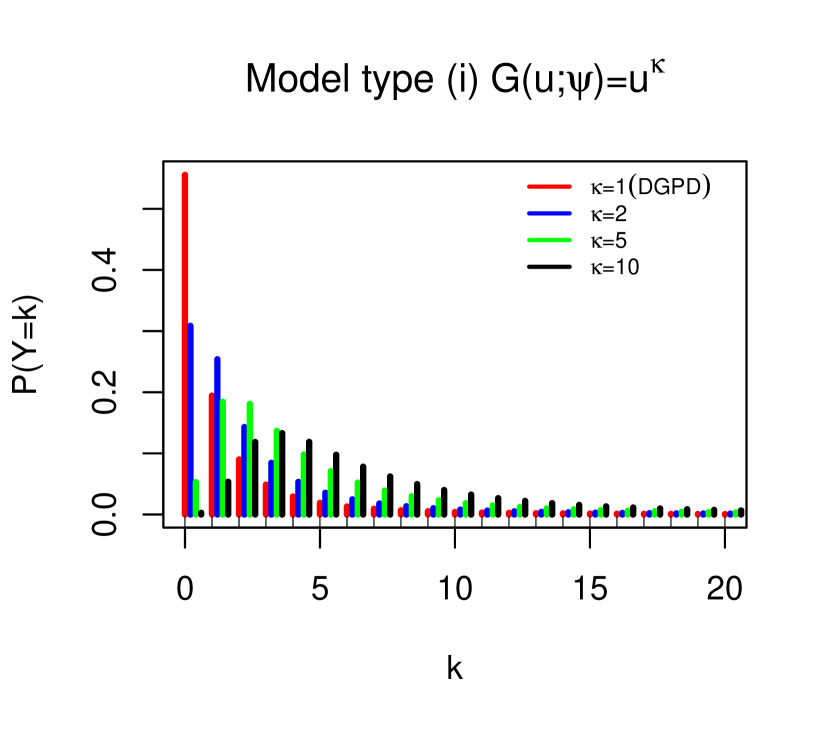
(a)

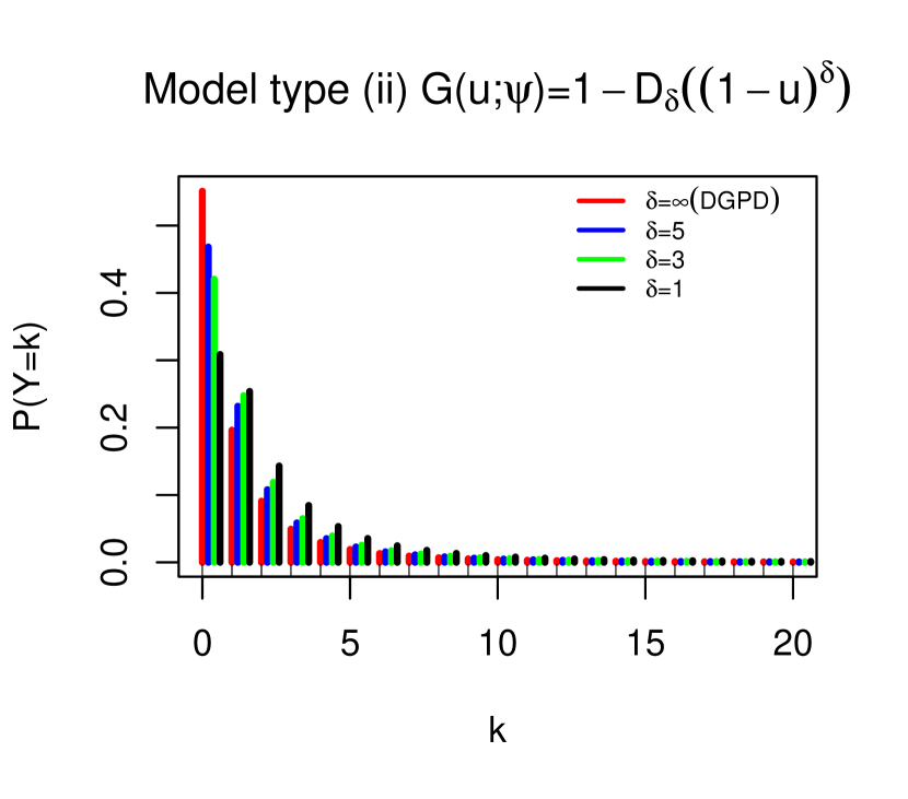
(b)

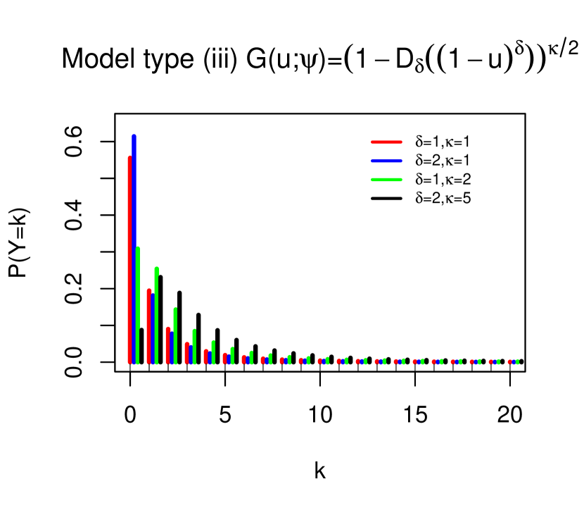
(c)

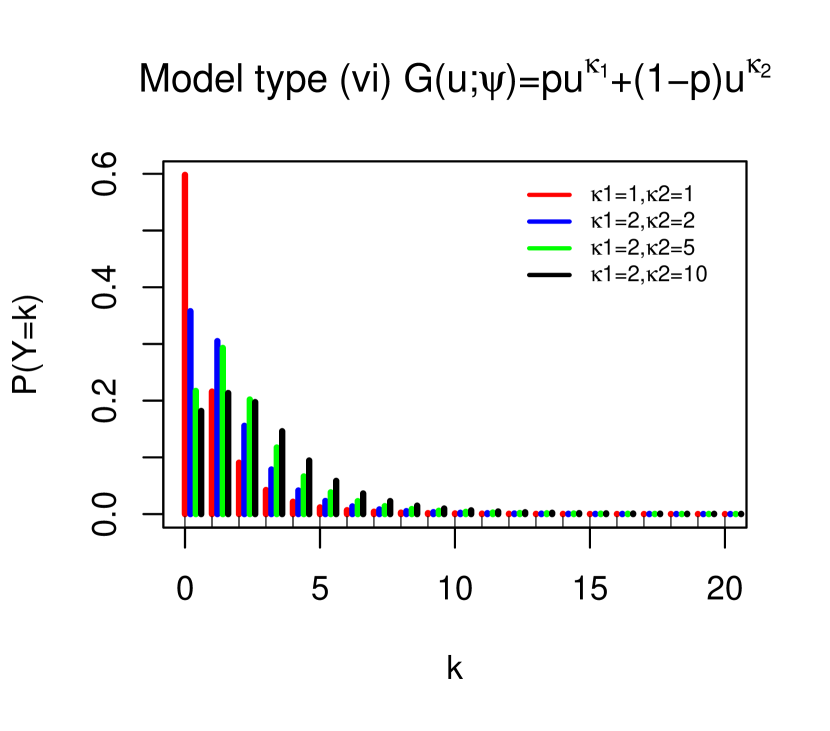
(d)

Figure 1: (a) Probability mass function corresponding to model in (5) type (i) for $\sigma=1,\xi=0.5$ and shape parameter for lower tail $\kappa=1,2,5,10$; (b) Probability mass function corresponding to model (5) combined with $G(u;\psi)=1-D_{\delta}(1-u)^{\delta}$ for $\sigma=1,\xi=0.5$ and $\delta=\infty,5,3,1$; (c) Probability mass function corresponding to model (5) combined with $G(u;\psi)=[1-D_{\delta}(1-u)^{\delta}]^{\kappa/2}$ for $\sigma=1,\xi=0.5$, $\delta=1,2$ and $\kappa=1,2,5$, and (d) Probability mass function corresponding to model in (5) combined with $G(u;\psi)=pu^{\kappa_{1}}-(1-p)u^{\kappa_{2}}$ for $\sigma=1,\xi=0.2$, $\kappa_{1}=1,2$ and $\kappa_{2}=1,2,5,10$.

The parametric family (iii) is supporting the lower tail of the distribution with $\kappa>0$ parameter. Interestingly, this family also tend to the DEGPD with parameters ($\kappa,\delta,\sigma$ and $\xi$). The $(\kappa,\delta$ and $\xi)$ represents the lower, central and the upper parts of the distribution, respectively, and $\sigma$ is a scale parameter as usual. In particular, Figure (1, c) showing the behavior of PMF of DEGPD linked with $G(u;\psi)=\left[1-D_{\delta}\{(1-u)^{\delta}\}\right]^{\kappa/2}$ at different settings of the parameters.

Overall, the all types of DEGPD discussed above with combination of different parametric families are more flexible for modeling discrete extremes except the DEGPD (ii). In fact, the DEGPD (ii) corresponding to parametric family (ii) has limited flexibility on lower tail.

In addition, a large number of zeros can be found in various practical application data sets. In that case, the usual statistical models with flexible lower tail cannot be adjusted for the excessive zeros, which complicates a precise statistical analysis. An investigation of the origins of these zeros is essential. The subsequent section will explain the zero inflation modeling framework.

2.2 Zero-inflated discrete extended generalized Pareto distribution

We follow Lambert (1992) and we suppose that $Z$ is observed with an excessive number of zeros relative to those observed under the DEGPD, the zero inflated distribution (ZIDEGPD) is defined in straightforward way as:

$$P(Z=m)=\left\{\begin{array}[]{ll}\pi+(1-\pi)G\left\{F\left(1,\sigma,\xi\right)\right\}&m=0\\ (1-\pi)\left[G\left\{F\left(m+1,\sigma,\xi\right)\right\}-G\left\{F\left(m,\sigma,\xi\right)\right\}\right]&m=1,2,\ldots\end{array}\right.$$ (8)

where $0\leq\pi\leq 1$ and the remaining parameters would be the same like DEGPD. It turns out that the CDF of ZIDEGPD is

$$P(Z\leq m)=\pi+(1-\pi)G\left\{F\left(m+1,\sigma,\xi\right)\right\},\qquad m\in\mathbb{N},$$ (9)

and the quantile function is

$$q_{p^{*}}=\left\{\begin{array}[]{lc}\lceil\frac{\sigma}{\xi}\left[\left\{1-G^{-1}(p^{*})\right\}^{-\xi}-1\right]\rceil-1,&\xi>0\\ \lceil{-\sigma\log\left\{1-G^{-1}(p^{*})\right\}}\rceil-1,&\xi=0\\ \end{array}\right.$$ (10)

with $0<p^{*}=(p-\pi)/(1-\pi)<1$. Again, the above expressions are quite simple and straightforward with existing four G families. The flexibility of the proposed extended versions is observed here through PMF with different lower tail parameters.

The parametric family (i) also leads to PMF of ZIDEGPD given in (8) with four parameters $(\pi,\kappa,\sigma$ and $\xi)$: $\pi$ is the proportion of zero observations in the sample that is inflating the data distribution and the interpretation of other parameters is same as DEGPD. Thus, the Figure (2, a) shows the behavior of PMF of ZIDEGPD with fixed zero-inflation, scale and upper tail shape parameters (i.e., $\pi=0.20,\sigma=1$ and $\xi=0.2$) and with different values of lower tail behaviors ($\kappa=1,2,5,10$). The zero-inflated DGPD is recovered when $\kappa=1$ with more proportion of zero values. Additional flexibility for low values with proportion of zero inflation is attained by varying $\kappa$. For instance, more flexibility on lower tail with zero inflation can be observed without losing upper tail behavior in Figure (2, a) when putting the value of $\kappa=10$ or $20$. The ZI Poisson and ZIDEGPD densities act similarly for small and moderate values, but the dissimilarity may rises in at upper tail.

The ZIDEGPD corresponding to parametric family (iv) have six parameters $(\pi,p,\kappa_{1},\kappa_{2},\sigma$ and $\xi)$ by following the restriction ($\kappa_{1}\leq\kappa_{2}$). It can be noticed from Figure (2, d) that the ZIDEGPD based on $G(u;\psi)=pu^{\kappa_{1}}+(1-p)u^{\kappa_{2}}$ is also a flexible and produce zero inflation when using $\pi=0.2$, $p=0.5$, $\sigma=1$, $\xi=0.2$, $\kappa_{1}=1,2$, different values of $\kappa_{2}$. Again, the density of ZI Poisson and ZIDEGPD show similar behaviour for small and moderate values, it may change at upper tail due to heavy tail of ZIDEGPD.

The ZIDEGPD proposed by using $G(u;\psi)=1-D_{\delta}\{(1-u)^{\delta}\}$) have four parameters $(\pi,\delta,\sigma$ and $\xi$) . Figure (2, b), describes the behaviour of PMF with fixed values of parameters $(i.e.,\pi=0.2,\sigma=1$ and $\xi=0.2)$ and with different values of $\delta$. The ZIDEGPD follow ZIDGPD when $\delta$ increases to infinity. It can be observed that the amount of zeros increases when $\delta$ increases. This behaves like ZIP at lower tail and at central part when the mean of ZIP is small. The disadvantage of this kind of ZIDEGPD is that it models only the central and upper part of the distribution, the lower tail behavior could not be estimated directly even though we have a zero inflation.

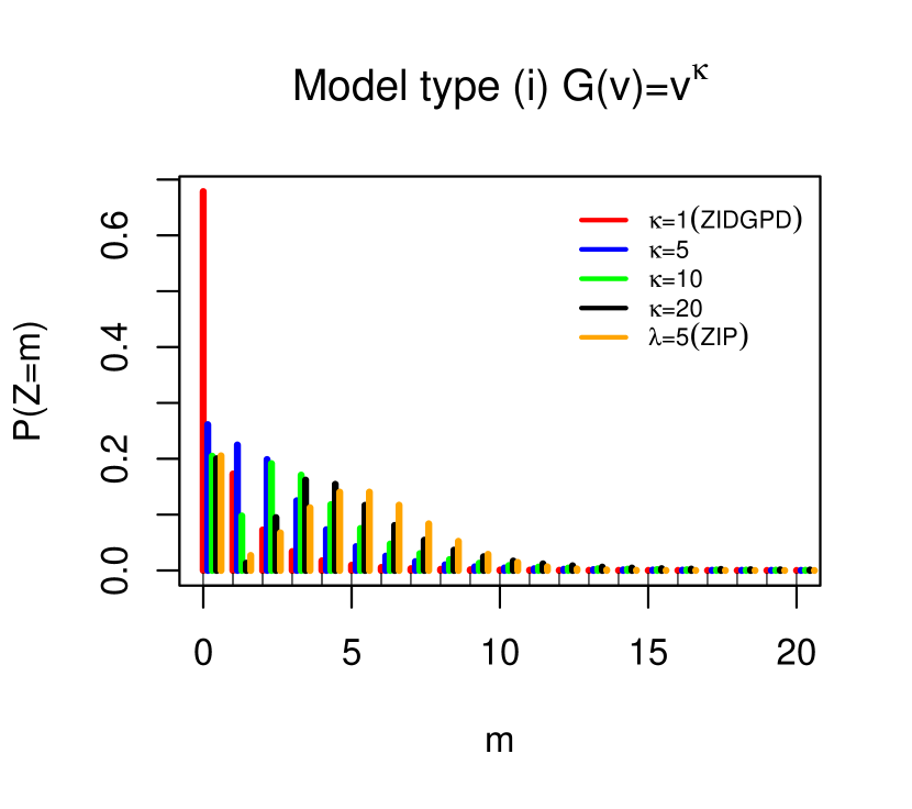
(a)

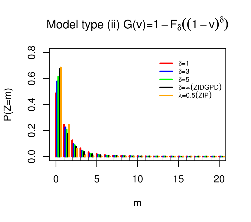
(b)

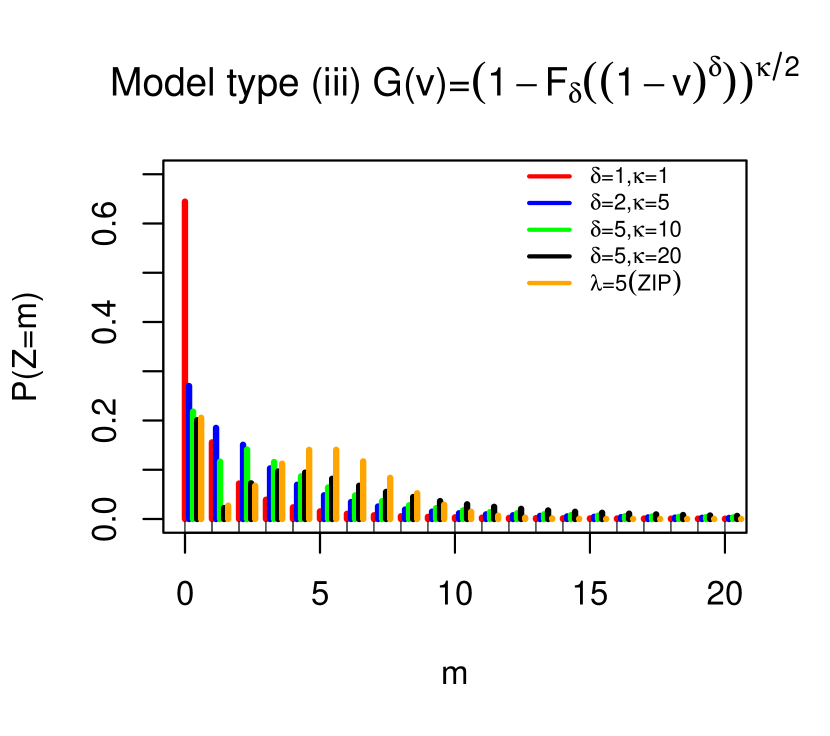
(c)

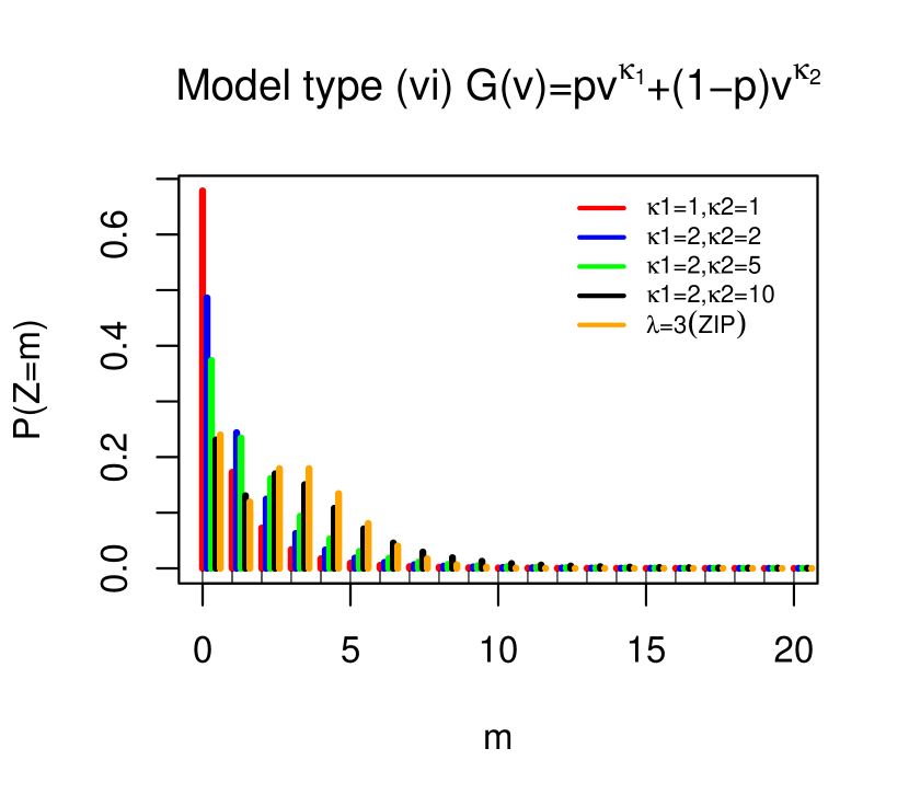
(d)

Figure 2: (a) Probability mass function corresponding to model in (8) with $G(u;\psi)=u^{\kappa}$ having $\pi=0.2,\sigma=1,\xi=0.2$ and shape parameter for lower tail $\kappa=1,5,10,20$; (b) Probability mass function corresponding to model in (8) combined with $G(u;\psi)=1-D_{\delta}(1-u)^{\delta}$ for $\pi=0.2,\sigma=1,\xi=0.2$ and $\delta=1,3,5,\infty$; (c) Probability mass function corresponding to model in (8) combined with $G(u;\psi)=[1-D_{\delta}(1-u)^{\delta}]^{\kappa/2}$ for $\pi=0.2,\sigma=1,\xi=0.2$, $\delta=1,2,5$ and $\kappa=1,5,10,20$, and (d) Probability mass function corresponding to model (8) combined with $G(u;\psi)=pu^{\kappa_{1}}-(1-p)u^{\kappa_{2}}$ for $\pi=0.2,p=0.5,\sigma=1,\xi=0.2$, $\kappa_{1}=1,2$ and $\kappa_{2}=1,2,5,10$. The orange lines represent the zero-inflated Poisson probability mass function with different setting of their parameter.

The proposed ZIDEGPD based on $G(u;\psi)=\left[1-D_{\delta}\{(1-u)^{\delta}\}\right]^{\kappa/2}$) have five parameters: $\pi$ supporting the proportion of zero values, the $(\kappa,\delta$ and $\xi)$ represents the lower, central and the upper parts of the distribution, respectively, and $\sigma$ is a scale parameter as usual. Figure (2, c) showing the behavior of PMF of ZIDEGPD linked with $G(u;\psi)=\left[1-D_{\delta}\{(1-u)^{\delta}\}\right]^{\kappa/2}$ at different settings of the parameters. The zero inflation also occurring when $\kappa$ increases. Again, the density shape is similar to ZIP at lower and central part of the distribution.

In general, all types of ZIDEGPD discussed above with support of different parametric families are flexible for both tails in modeling of zero inflated discrete extremes. In fact, the ZIDEGPD (ii) corresponding to parametric family (ii) has limited flexibility on lower tail, but $\pi$ parameter explain zero proportion more correctly.

3 Generalized additive modelling

The objective of this section is to propose regression-based discrete extreme models by letting the parameters of discrete extreme models vary with covariates. In a continuous framework, modeling continuous variables via extreme value models approximations, it is very appealing to employ techniques that allow for the incorporation of flexible forms of dependence on covariates. Davison and Smith (1990) used such types of models for modeling the size and occurrence of excesses over a high threshold through GPD. Pauli and Coles (2001) proposed smooth models for extreme value distribution parameters based on penalized likelihood. Later on, Chavez-Demoulin and Davison (2005) used Generalized Additive Model (GAM) that was originally proposed by Hastie and Tibshirani (1990) to estimate flexibly GPD parameters with an orthogonal reparametrization. Yee and Stephenson (2007) developed vector generalized additive models to model generalized extreme value distribution parameters as linear or smooth functions of covariates. Vector generalized additive models can easily be implemented in an R package called VGAM. More recently, Youngman (2019) models threshold exceedances with GPD parameters of GAM forms. Generally, the GAM form models characteristically reflect additive smooths representations with splines.

In the sequel we denote the vector of parameters $(\xi,\sigma,\psi^{T})^{T}$ or $(\xi,\sigma,\psi^{T},\pi)^{T}$ with $\theta=(\theta_{1},...,\theta_{d})^{T}$. In practice, the parameters of the distribution of $Y$ or $Z$ may depend on some covariates $\bm{x}$, i.e. $\theta(\bm{x})=(\theta_{1}(\bm{x}),\ldots,\theta_{d}(\bm{x}))^{T}$. The specification is an instance of a distributional regression model (Stasinopoulos et al., 2018).

For relating the distributional parameters $(\theta_{1}(\bm{x}),\ldots,\theta_{d}(\bm{x}))$ to the covariates, we consider additive predictors of the form

$$\eta_{i}(\bm{x})=s_{i1}(\bm{x})+\cdots+s_{iJ_{i}}(\bm{x})$$ (11)

where $s_{i1}(\cdot),\ldots,s_{iJ_{i}}(\cdot)$ are smooth functions of the covariates $\bm{x}$. The predictors are linked to the distributional parameters via known monotonic and twice differentiable link functions $h_{i}(\cdot)$.

$$\theta_{i}(\bm{x})=h_{i}(\eta_{i}(\bm{x})),\qquad i=1,\ldots,d$$ (12)

In the case of model with $G(u;\psi)=u^{\kappa}$, common link functions are

$$\xi(\bm{x})=\eta_{\xi}(\bm{x}),\quad\sigma(\bm{x})=\exp(\eta_{\sigma}(\bm{x})),\quad\kappa(\bm{x})=\exp(\eta_{\kappa}(\bm{x})),\quad\pi(\bm{x})=\exp\left(\frac{\eta_{p}(\bm{x})}{1+\eta_{p}(\bm{x})}\right)$$

The functions $s_{ij}$ in (11) are approximated in terms of basis function expansions

$$s_{ij}(\bm{x})=\sum_{k=1}^{K_{ij}}\beta_{ij,k}B_{k}(\bm{x}),$$ (13)

where $B_{k}(\bm{x})$ are the basis functions and $\beta_{ij,k}$ denote the corresponding basis coefficients. These basis can be of different types (see Wood, 2017, for instance). The basis function expansions can be written as $s_{ij}(\bm{x})=\bm{t}_{ij}(\bm{x})^{T}\bm{\beta}_{ij}$ where $\bm{t}_{ij}(\bm{x})$ is still a vector of transformed covariates that depends on the basis functions and $\bm{\beta}_{ij}=(\beta_{ij,1},\ldots,\beta_{ij,K_{ij}})^{T}$ is a parameter vector to be estimated.

To estimate the parameters of the proposed models, the maximum likelihood estimation (MLE) method is practiced. Let $y_{1},\ldots,y_{n}$ be $n$ independent observations from (5) and $\bm{x}_{1},\ldots,\bm{x}_{n}$ the related covariates. The log-likelihood function is given by,

$$l(\bm{\beta})=\sum_{i=1}^{n}\log\left[G(F(y_{i}+1;\sigma(\bm{x}_{i}),\xi(\bm{x}_{i}));\psi(\bm{x}_{i}))-G(F(y_{i};\sigma(\bm{x}_{i}),\xi(\bm{x}_{i}));\psi(\bm{x}_{i}))\right].$$ (14)

where $\bm{\beta}$ collects all unknown coefficient $\beta_{ijk}$ of the basis expansions.

Instead if we consider $n$ independent observations $z_{1},\ldots,z_{n}$ from (8) we get

$$l(\bm{\beta}) = \sum_{i=1}^{n}I_{0}(z_{i})\log\left[\pi(\bm{x}_{i})+(1-\pi(\bm{x}_{i}))G(F(1;\sigma(\bm{x}_{i}),\xi(\bm{x}_{i}));\psi(\bm{x}_{i}))\right]+$$ (15)

$$+\sum_{i=1}^{n}(1-I_{0}(z_{i}))\log(1-\pi(\bm{x}_{i})))\times$$

$$\left[G(F(z_{i}+1;\sigma(\bm{x}_{i}),\xi(\bm{x}_{i}));\psi(\bm{x}_{i}))-G(F(z_{i};\sigma(\bm{x}_{i}),\xi(\bm{x}_{i}));\psi(\bm{x}_{i}))\right].$$

Derivatives with respect unknown parameters of DEPGD and ZIDEGPD can be solved by standard numerical techniques to obtain the maximum likelihood estimators for unknown parameters.

To ensure regularization of the functions $s_{ij}(\bm{x})$ so-called penalty terms are added to the objective log-likelihood function. Usually, the penalty for each function $s_{ij}(\bm{x})$ are quadratic penalty $\lambda\bm{\beta}_{ij}^{T}\bm{G}_{ij}(\bm{\lambda}_{ij})\bm{\beta}_{ij}$ where $\bm{G}_{ij}(\bm{\lambda}_{ij})$ is a known semi-definite matrix and the vector $\bm{\lambda}_{ij}$ regulates the amount of smoothing needed for the fit. A special case is when $\bm{G}_{ij}(\bm{\lambda}_{ij})=\lambda_{ij}\bm{G}_{ij}$. Therefore the type and properties of the smoothing functions are controlled by the vectors $\bm{x}_{ij}(\bm{x})$ and the matrices $\bm{G}_{ij}(\bm{\lambda}_{ij})$.

The penalized log-likelihood function for the latter models reads:

$$l_{p}(\bm{\beta})=l(\bm{\beta})-\frac{1}{2}\sum_{i=1}^{d}\sum_{j=1}^{J_{i}}\bm{\beta}_{ij}^{T}\bm{G}_{ij}(\bm{\lambda}_{ij})\bm{\beta}_{ij}$$ (16)

where $l(\bm{\beta})$ is the log-likelihood function (14) or (15).

To fit DEGPD and ZIDEGPD with GAM forms, we have written a R code that implements the distributions as “new families” for evgam R package (Youngman, 2020). An example of R code with the name “Fit_degpd_zidegpd.R” and the complete source code of the function is provided on the GitHub https://github.com/touqeerahmadunipd/degpd-and-zidegpd.

4 Simulation study

4.1 Discrete extended Generalized Pareto distribution

This section deals with a simulation study planned to evaluate maximum likelihood estimate (MLE) performance. Different settings of parameters are tried to test each model. Moreover, the scale and upper tail shape parameters are permanently set to ($\sigma=1,\xi=0.2$) for all four models, respectively. The sample size $n=1000$ with $10^{4}$ replications are used to calculate root mean square errors (RMSEs) corresponding to each model. Remaining parameters of the proposed models are set in the following way

• $G(u;\psi)=u^{\kappa}$ with lower tail parameter $\kappa$ = 1, 2, 3, 10.

• $G(u;\psi)=1-D_{\delta}\{(1-u)^{\delta}\}$, with $\delta$ = 0.5, 1, 2, 5.

• $G(u;\psi)=\left[1-D_{\delta}\{(1-u)^{\delta}\}\right]^{\kappa/2}$ with $\delta$ = 0.5, 1, 2, 5 and $\kappa$ = 1, 2, 3, 10.

• $G(u;\psi)=pu^{\kappa_{1}}+(1-p)u^{\kappa_{2}}$ with $p=0.5$, $\kappa_{1}$ = 1, 2, 3, 10 and $\kappa_{2}$ = 2, 3, 10, 20.

The boxplots of the MLEs are constructed to assess the models performance for the above representative cases. Figure 3 shows the boxplots of estimated parameters conforming to all four models with different simulation settings. Figure 3(a) show MLEs of DEGPD based on parametric family $G(u;\psi)=u^{\kappa}$ with true parameter settings (i.e., $\kappa=1,2,5,10$, $\sigma=1$, and $\xi=0.2$). In addition, the horizontal red line in each boxplot represent the true parameters. More precisely, Figure 3(a) indicate that the MLEs of DEGPD (i) are quite reasonable with less variability.

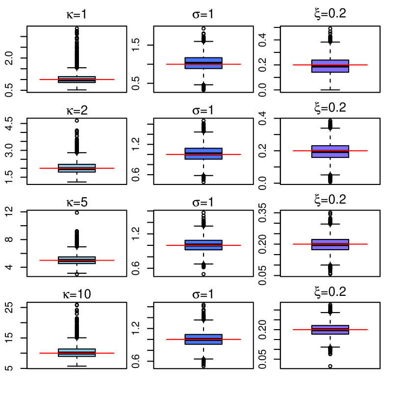
(a) $G(u;\psi)=u^{\kappa}$

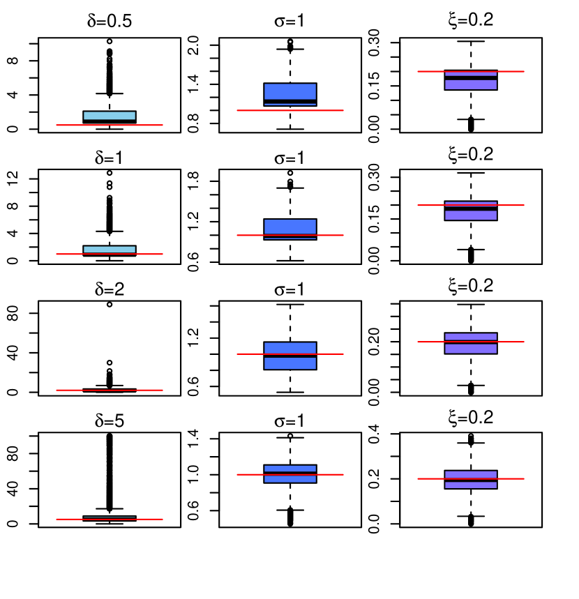
(b) $G(u;\psi)=1-D_{\delta}\{(1-u)^{\delta}\}$

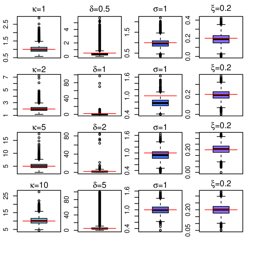
(c) $G(u;\psi)=\left[1-D_{\delta}\{(1-u)^{\delta}\}\right]^{\kappa/2}$

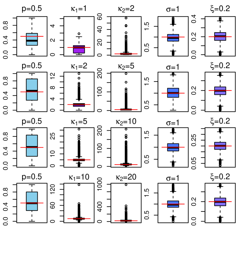
(d) $G(u;\psi)=pu^{\kappa_{1}}+(1-u)v^{\kappa_{2}}$

Figure 3: Boxplots of maximum likelihood estimates of parameters of each model from $n=500$ with $10^{4}$ replication at different parameters settings: $\mathbb{(a)}$ corresponds to model type (i), $\mathbb{(b)}$ corresponds to model type (ii), $\mathbb{(c)}$ corresponds to model type (iii), and $\mathbb{(d)}$ corresponds to model type (iv).

Figure 3(b) report a much variability in the estimates of parameter $\delta$ when we increase true value of $\delta$. This may happen due to skewness parameter $\delta$. Skewness parameters like $\delta$ and $\kappa_{2}$ are hard to estimate by the MLE method, this was observed by Naveau et al. (2016) for extended generalized Pareto distributions, Sartori (2006) for the skew-normal and Ribereau et al. (2016) for skew generalized extreme value case.

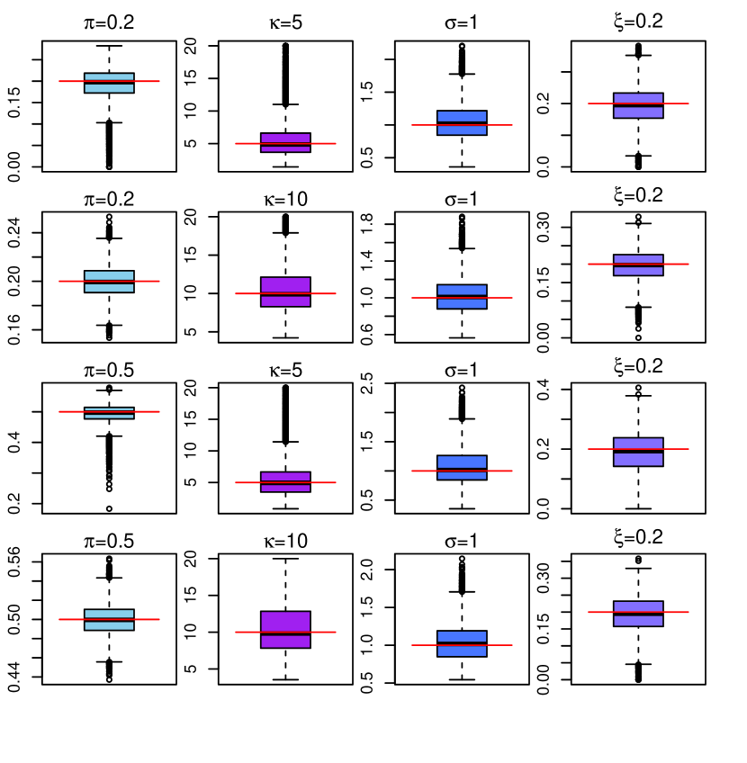
(a) $G(u;\psi)=u^{\kappa}$

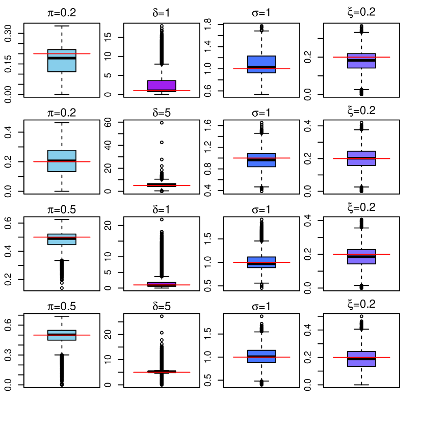
(b) $G(u;\psi)=1-D_{\delta}\{(1-u)^{\delta}\}$

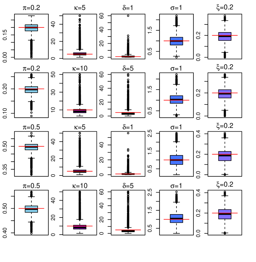
(c) $G(u;\psi)=\left[1-D_{\delta}\{(1-u)^{\delta}\}\right]^{\kappa/2}$

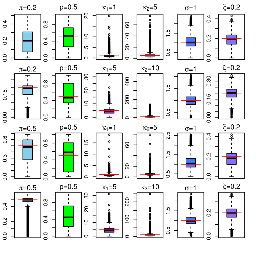
(d) $G(u;\psi)=pu^{\kappa_{1}}+(1-p)u^{\kappa_{2}}$

Figure 4: $\mathbb{(a)}$ Boxplots of maximum likelihood estimates of parameters of each ZIDEGPD model from $n=1000$ with $10^{4}$ replication at different parameters settings: $\mathbb{(a)}$ corresponds to model type (i), $\mathbb{(b)}$ corresponds to model type (ii), $\mathbb{(c)}$ corresponds to model type (iii), and $\mathbb{(d)}$ corresponds to model type (iv).

Similarly, Figure 3(c) shows again $\delta$ is out perform when true value increases. Figure 3(d) shows the MLEs for all parameter are reasonable with variability seen in $\kappa_{2}$ and sometimes in $\kappa_{1}$. Again, this may possible due to appearance of $\kappa_{2}$ as skewness parameter (Naveau et al., 2016).

For further investigation, the RMSEs of models parameters for each configuration are given in Table 1. Overall, the findings of the table show that the maximum likelihood estimator performed well for model type (i) when the lower shape parameter $\kappa$ increases. Model type (ii) highlights that the MLEs are sensible when threshold tuning parameter $\delta<5$. The RMSEs in respect to model type (iii) show that the MLEs are poor when $\delta>1$. Finally, the case of model type (iv) intensifies that the parameters $\kappa_{1}$ and $\kappa_{2}$ entail much variability, especially when $\kappa_{1}>2$ and $\kappa_{2}>5$.

Table 1: Root mean square errors of parameter estimates of DEGPD found from $10^{4}$ independent data sets of size $n=1000$. TRUE represent the true values of the parameters used during simulation.

$G(u;\psi)=u^{\kappa}$
$\kappa$	RMSE	$\sigma$	RMSE	$\xi$	RMSE
1	0.24	1	0.21	0.20	0.07
2	0.35	1	0.16	0.20	0.05
5	0.76	1	0.12	0.20	0.04
10	2.05	1	0.13	0.20	0.03
$G(u;\psi)=1-D_{\delta}\{(1-u)^{\delta}\}$
$\delta$	RMSE	$\sigma$	RMSE	$\xi$	RMSE
0.5	1.52	1	0.33	0.20	0.06
1	1.36	1	0.22	0.20	0.06
2	2.13	1	0.20	0.20	0.06
5	19.64	1	0.16	0.20	0.06
$G(u;\psi)=\left[1-D_{\delta}\{(1-u)^{\delta}\}\right]^{\kappa/2}$
$\delta$	RMSE	$\kappa$	RMSE	$\sigma$	RMSE	$\xi$	RMSE
0.5	0.42	1	0.20	1	0.20	0.20	0.06
1	0.94	2	0.39	1	0.20	0.20	0.05
2	1.94	5	1.01	1	0.19	0.20	0.04
5	30.15	10	2.33	1	0.13	0.20	0.04
$G(u;\psi)=pu^{\kappa_{1}}+(1-p)u^{\kappa_{2}}$
$p$	RMSE	$\kappa_{1}$	RMSE	$\kappa_{2}$	RMSE	$\sigma$	RMSE	$\xi$	RMSE
0.5	0.28	1	0.58	2	1.83	1	0.23	0.20	0.06
0.5	0.32	2	0.98	5	6.43	1	0.26	0.20	0.06
0.5	0.32	5	2.13	10	12.19	1	0.23	0.20	0.04
0.5	0.30	10	4.62	20	25.47	1	0.23	0.20	0.04

4.2 Zero-inflated discrete extended Generalized Pareto distribution

To evaluate maximum likelihood estimator for ZIDEGPD models, the simulation study have been conducted with different configurations of parameters. The scale and upper tail shape parameters are fixed to $\sigma=1$ and $\xi=0.2$ for all four models, respectively. Similar to DEGPD, the sample size $n=1000$ with $10^{4}$ replications are used to calculate RMSEs for each model. The other parameters of the proposed ZIDEGPD are chosen as

• $G(u;\psi)=u^{\kappa}$ with lower tail parameter $\kappa$ = 5, 10

• $G(u;\psi)=1-D_{\delta}\{(1-u)^{\delta}\}$, with $\delta$ = 1, 5.

• $G(u;\psi)=\left[1-D_{\delta}\{(1-u)^{\delta}\}\right]^{\kappa/2}$ with $\delta$ = 1, 5 and $\kappa$ =5, 10.

• $G(u;\psi)=pu^{\kappa_{1}}+(1-p)u^{\kappa_{2}}$ with $p=0.5$, $\kappa_{1}$ = 1, 5 and $\kappa_{2}$ = 5, 10.

The zero inflation parameter (i.e proportion of zeros) $\pi$ is considered $0.2$ and $0.5$ for all models, respectively.

Figure 4 clearly shows that the parameter of ZIDEPD are estimated correctly for $G(u;\psi)=u^{\kappa}$ even though when proportion of zeros is higher. Similar to DEGPD, the estimates of $\delta$ of ZIDEGPD model (ii), $\kappa$ and $\delta$ of ZIDEGPD model (iii) and $\kappa_{1}$ and $\kappa_{2}$ of ZIDEGPD model (iv) showing more variability. This is already we noted for DEGPD cases.

Similar to DEGPD, we check the performance of maximum likelihood estimator for ZIDEGPD by observing RMSEs of the parameters. We found that the the $\delta$ parameter involved in model type (ii) and model type (iii) and $\kappa_{2}$ parameter of model type (iv) entail much variability when estimated by MLE. Similar characteristics have already being noted in DEGPD models. In addition, we found the ZIDEGPD based on $G(u;\psi)=u^{\kappa}$ is more reliable than other models. Information regarding RMSEs of ZIDEGPD parameters is reported in ”Supplementary materials”.

5 Real data applications

This section discusses two applications of the proposed models Section 2 and 3. Firstly we shall consider a dataset on automobile insurance claims. Then we consider the avalanches data of Haute-Maurienne massif of French Alps with environmental variables as covariates.

5.1 Discrete extended generalized Pareto distribution

We apply proposed DEGPD models to automobile insurance claims data of the companies of New York city recorded from 2009 to 2020. The data is basically recorded under Department of Financial Services (DFS) rank automobile insurance companies running a business in New York State based on the number of consumer complaints upheld against them as a percentage of their total business over two years. Complaints typically include problems like delays in the payment of no-fault claims and nonrenewal of policies. Insurers with the least upheld complaints per million dollars of premiums stand at the top. The data is freely available on the given website https://www.ny.gov/programs/open-ny. The frequency distribution of the data ($1942$ observations) is depicted in Figure 5.

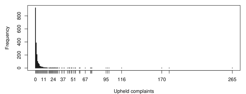
Figure 5: Frequency distribution of upheld complaints of automobile insurance companies at New York city (2009-2020).

Table 2: Estimated parameters for extended versions of discrete Pareto distribution with all four parametric families fitted to insurance complaints data of New York City. Standard errors are reported between parenthesis. The bootstrap confidence intervals at level 95% are reported between square brackets.

$G(u;\psi)=u^{\kappa}$
$\kappa$	$\sigma$	$\xi$
1.41	0.80	0.73
(0.37)	(0.20)	(0.05)
$[1.00,2.35]$	[0.43, 1.22]	[0.61, 0.83]
$G(u;\psi)=1-D_{\delta}\{(1-u)^{\delta}\}$
$\delta$	$\sigma$	$\xi$
0.006	0.36	0.65
(0.86)	(0.15)	(0.04)
$[0.00,1.46]$	[0.33, 0.61]	[0.60, 0.80]
$G(u;\psi)=\left[1-D_{\delta}\{(1-u)^{\delta}\}\right]^{\kappa/2}$
$\kappa$	$\delta$	$\sigma$	$\xi$
1.61	0.11	0.49	0.65
(0.42)	(0.65)	(0.24)	(0.07)
$[1.05,2.79]$	[0.00, 1.68]	[0.27, 1.20]	[0.55, 0.83]
$G(u;\psi)=pu^{\kappa_{1}}+(1-p)u^{\kappa_{2}}$
$p$	$\kappa_{1}$	$\kappa_{2}$	$\sigma$	$\xi$
0.11	0.01	2.08	0.63	0.73
(0.12)	(0.44)	(2.59)	(0.16)	(0.05)
$[0.00,0.46]$	[0.00, 1.59]	[1.44, 10.66]	[0.20, 0.84]	[0.64, 0.83]

Moreover, the DEGPD and ZIDEGPD based on parametric families (i), (ii), (iii) and (iv) are fitted to the upheld complaints count data. Results of the fitted the DEGPD models with their standard errors and bootstrap confidence intervals are given in Table 2. AIC and BIC associated with fitted DEGPD and ZIDEGPD models and Chi-square goodness-of-fit test statistic along with p-values are reported in Table 3. According to AIC and BIC values given Table 3, the DEGPD (i) and ZIDEGPD (i) with $G(u;\psi)=u^{\kappa}$ performing better for this specific data example. DEGPD type (ii) fitting is also quite reasonable to the upheld complaints data with smaller estimate of the parameter $\delta$, but the Model type (ii) has restricted flexibility on its lower tail. This is kind of disadvantage of model type (ii)(Naveau et al., 2016). In case of zero-inflation in the data the ZIDEGPD based on $G(u;\psi)=1-D_{\delta}\{(1-u)^{\delta}\}$ may perform better by the reason that it has an addition parameter which represent the zero proportion separately. The fitting of DEGPD type (iii) with $G(u;\psi)=\left[1-D_{\delta}\{(1-u)^{\delta}\}\right]^{\kappa/2}$ and DEGPD type (iv) with $G(u;\psi)=pu^{\kappa_{1}}+(1-p)u^{\kappa_{2}}$ is also quite sensible with lower AIC and BIC value as compared to ZIDEGPD type (iii) and ZIDEGPD type (iv). But $\kappa_{2}$ parameter of DEGPD type (iv) have gained more variability, which is also pointed by Naveau et al. (2016) in continuous framework. In addition, q-q plots show that all types of DEGPD are fitted reasonably well to upheld complaints data of New York city. Furthermore, the p-values of chi-square test statistic corresponding to each of DEGPD and ZIDEGPD indicate that the fitting of the models proposed in section 2 is pretty good to this specific real data example. Based on AIC and BIC, we prefer the DEGPD of type (i) for upheld complaints data.

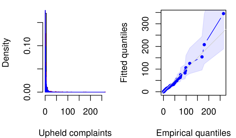
(a) $G(u;\psi)=u^{\kappa}$

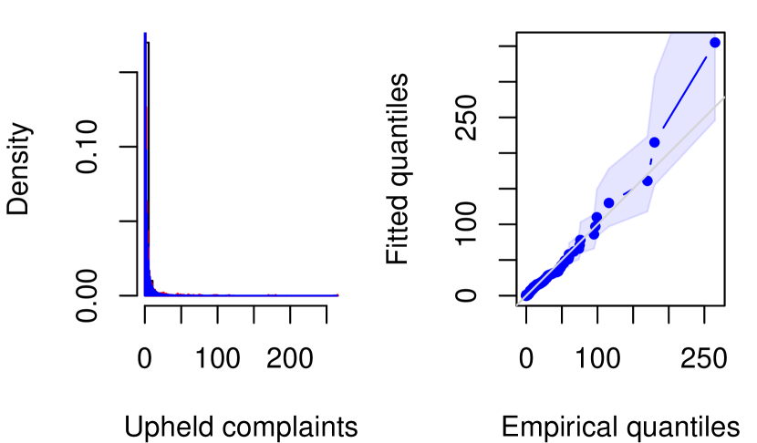
(b) $G(u;\psi)=1-D_{\delta}\{(1-u)^{\delta}\}$

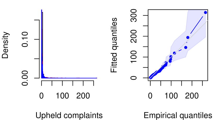
(c) $G(u;\psi)=\left[1-D_{\delta}\{(1-u)^{\delta}\}\right]^{\kappa/2}$

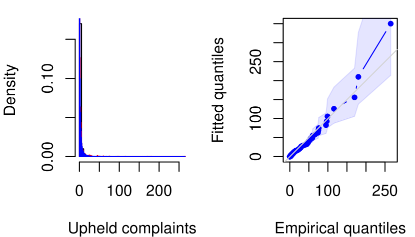
(d) $G(u;\psi)=pu^{\kappa_{1}}+(1-p)u^{\kappa_{2}}$

Figure 6: Quantile-quantile plots of the fitted models with $95\%$ bootstrap-based confidence intervals

Table 3: AIC and BIC associated with the fitted DEGPD and ZIDEGPD along with Chi-square goodness-of-fit test. P-value are reported between parenthesis.

	AIC		BIC		Chi-square
Model	DEGPD	ZIDEGPD	DEGPD	ZIDEGPD	DEGPD	ZIDEGPD
(i)	7290.93	7291.40	7307.65	7313.69	0.20 (0.99)	0.18 (0.99)
(ii)	7291.88	7293.05	7308.60	7315.34	0.19 (0.99)	0.20 (0.99)
(iii)	7293.36	7294.56	7315.64	7322.42	0.20 (0.99)	0.20 (0.99)
(iv)	7294.45	7297.56	7322.30	7330.99	0.20 (0.99)	0.22 (0.99)

5.2 GAM forms applications of DEGPD and ZIDEGPD to avalanches data

In the Alpine regions, snow avalanches with extreme frequency or magnitude are considered a life-threatening hazard. Avalanches are usually caused by severe storms that bring high snowfalls coupled with snow drifting, but strong variations of environmental factors (e.g., temperature, wind, humidity and precipitation etc.) causing snow melt and/or fluctuations of the freezing point can also be involved (Evin et al., 2021). It is crucial to anticipate the future avalanches activity in the short-term and long-term management. Since extreme events have potentially terrible consequences, it is crucial to assess their statistical characteristics correctly. To this end, we try to highlight avalanches events over a short period of time with the help of newly proposed extreme value models. In particular, we intend to quantify how weather-related variables affect the probability of avalanche occurrence each day.

The Enquête Permanente sur les Avalanches (EPA) collected avalanche data from the French Alps, which has monitored about 3900 paths since the early 20th century (see Mougin, 1922; Evin et al., 2021). Quantitative (run out elevations, deposit volumes, etc.) and qualitative (flow regime, snow quality, etc.) information is collected for each event. It varies in quality from time to time depending on the local observers (mostly forestry rangers). Natural avalanche activity is also uncertain because records tend to record paths visible from valleys, so high elevation activity may be underestimated.

We consider the dataset in Dkengne et al. (2016) and in particular the three day moving sum of daily number of avalanche events recorded from February 1982 to April 2021. Environmental covariates (see Table 4) has been downloaded from https://power.larc.nasa.gov/data-access-viewer/ by specifying latitude and longitude information. Then, the moving median of the previous three days was considered for each of them.

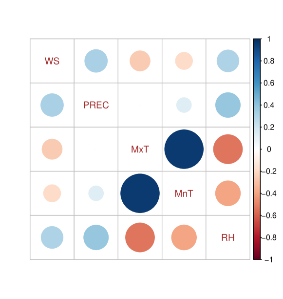
Figure 7: Correlation among covariates for avalanches data.

Table 4: Detailed information of covariates

Name	Definition
WS	maximum wind speed at 10 meters (m/s)
PREC	precipitation (mm/day)
MxT	maximum temperature at 2 Meters (Co)
MnT	minimum temperature at 2 Meters (Co)
RH	relative humidity at 2 Meters (%).

Figure 7 displays correlation plot among the covariates, highlighting, maximum temperature (MxT) and minimum temperature (MnT) are positively strong correlated, while precipitation (PREC) have no significant correlation with MxT. On the other hand, the relative humidity (RH) have moderate positive correlation with wind speed (WS) and PREC while it has weak negative correlation with temperature variables. Further, wind speed and precipitation have weak correlation with minimum and maximum temperature variables. Backward variable selection procedure based on AIC were performed for DEGPD model under the GAM form, using using evgam function with our own developed code. A preliminary study showed that a constant model is numerically preferred for lower shape parameter ($\kappa$ and $\kappa_{1}$), threshold tuning parameters ($\delta$ and $\kappa_{2}$) and upper shape parameter $\xi$.

After comparing different combinations of the covariates, we found WS, MxT, PREC and RH are more appropriate to use as covariates. It turned out that the models with the lowest AIC are

$$\begin{array}[]{lcl}\mbox{Model type (i)}&:&\kappa=cst;\quad\sigma=s(WS)+s(MxT)+s(PREC)+s(RH);\quad\xi=cst\\ \mbox{Model type (ii)}&:&\delta=cst;\quad\sigma=s(WS)+s(MxT)+s(PREC)+s(RH);\quad\xi=cst\\ \mbox{Model type (iii)}&:&\kappa=cst;\quad\delta=cst;\quad\sigma=s(WS)+s(MxT)+s(PREC)+s(RH);\quad\xi=cst\\ \mbox{Model type (iv)}&:&p=cst;\quad\kappa_{1}=cst;\quad\kappa_{2}=cst;\\ &&\sigma=s(WS)+s(MxT)+s(PREC)+s(RH);\quad\xi=cst\end{array}$$

where $s(\cdot)$ indicates the smoothed predictor.

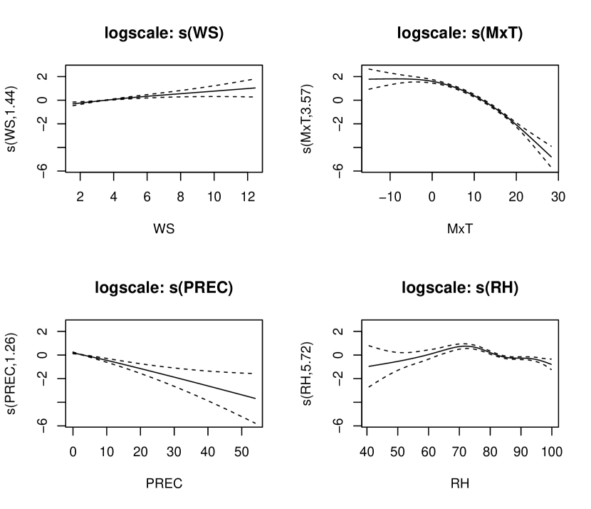
Figure 8: Estimated non-parametric effects of covariates in the $\sigma$ component of DEGPD model type (i).

Table 5: Estimated coefficients and smooth terms for GAM form DEGPD models fitted to avalanches data.

Model type (i) $G(u;\psi)=u^{\kappa}$
Parameter (intercept)	Estimate	Std.Error	t value	P-value
$\log(\kappa)$	-1.83	0.06	-32.38	$<$2e-16
$\log(\sigma)$	0.2	0.1	2.06	0.0197
$\log(\xi)$	-0.54	0.08	-6.88	2.93e-12
** Smooth terms for $\log(\sigma)$ **
$\log(\sigma)$	edf	max.df	Chi.sq	Pr($>|t|$)
s(WS)	1.44	4	22.01	8.66e-06
s(MxT)	3.57	4	663.24	$<$2e-16
s(PREC)	1.26	4	33.94	2.91e-08
s(RH)	5.72	9	79.14	9.9e-15
Model type (ii) $G(u;\psi)=1-D_{\delta}\{(1-u)^{\delta}\}$
Parameter (intercept)	Estimate	Std.Error	t value	P-value
$\log(\delta)$	4.72	1.28	3.7	0.000109
$\log(\sigma)$	-2.52	0.07	-34.84	$<$2e-16
$\log(\xi)$	0.14	0.03	4.94	3.89e-07
** Smooth terms for $\log(\sigma)$ **
$\log(\sigma)$	edf	max.df	Chi.sq	Pr($>|t|$)
s(WS)	1.90	4	31.12	3.75e-07
s(MxT)	3.52	4	528.98	$<$2e-16
s(PREC)	1.27	4	38.59	1.07e-08
s(RH)	6.30	9	59.21	8.61e-11
Model type (iii) $G(u;\psi)=\left[1-F_{\delta}\{(1-u)^{\delta}\}\right]^{\kappa/2}$
Parameter (intercept)	Estimate	Std.Error	t value	P-value
$\log(\kappa)$	-0.62	0.18	-3.4	0.000339
$\log(\delta)$	4.82	0.67	7.24	2.3e-13
$\log(\sigma)$	-0.62	0.29	-2.15	0.0158
$\log(\xi)$	-0.13	0.09	-1.39	0.0819
** Smooth terms for $\log(\sigma)$ **
s(WS)	1.78	4	29.29	4.66e-07
s(MxT)	3.61	4	562.36	$<$2e-16
s(PREC)	1.31	4	49.93	5.2e-10
s(RH)	6.07	9	47.71	1.3e-08
Model type (iv) $G(u;\psi)=pu^{\kappa_{1}}+(1-p)u^{\kappa_{2}}$
Parameter (intercept)	Estimate	Std.Error	t value	P-value
$\text{logit}(p)$	4.89	0.33	14.69	$<$2e-16
$\log(\kappa_{1})$	-1.84	0.06	-31.88	$<$2e-16
$\log(\kappa_{2})$	3.5	0.41	8.51	$<$2e-16
$\log(\sigma)$	0.17	0.1	1.66	0.0484
$\log(\xi)$	-0.86	0.13	-6.78	6.07e-12
** Smooth terms for $\log(\sigma)$ **
s(WS)	1.67	4	19.68	3.08e-05
s(MxT)	3.57	4	623.83	$<$2e-16
s(PREC)	1.05	4	35.18	4.71e-09
s(RH)	5.67	9	80.50	5.31e-15

We fitted all four DEGPD GAM form models to response variable (i.e. avalanches counts) with above selected covariates. The result of fitted models are given in Table 5. It can be observed from Table 5 that parametric and nonparametric terms for DEGPD GAM form models are statistically significant except the shape parameter in DEGPD type (iii). In addition, during estimation, much variability has been seen in constant parameters $\delta$ and $\kappa_{2}$. This may possible due to the appearance of $\delta$ and $\kappa_{2}$ as skewness parameters of the model (Naveau et al., 2016). Figure 8 shows the corresponding estimated functions of DEGPD type (i) model for the regressors that included as a nonparametric terms in model for the effect the environmental variables. To this end, the included nonparametric term is significant and have similar behavior for all models. Based on the results of all four models, a broad interpretation of the finding that the temperature and relative humidity seems to better explain the avalanches occurrence as compared to wind and precipitation. Possibly, the fluctuation in temperature may cause more avalanches coupled with snow drifting. Furthermore, we also fitted ZIDEGPD GAM form models looking at possible zero inflation in the avalanches data. A slight improvement is noted in ZIDEGPD type (i) and (iii). We found that parameter $\pi$ in ZIDEGPD type (ii) is not significant. This is possible due to much variation gained by $\delta$ parameter. The results about the ZIDEGPD model can be found in Supplementary material.

Further, when comparing our proposed models, the GAM forms DEGPD and ZIDEGPD type (i) and type (iii) overall performed well for the avalanches data. It may possible the other proposed models perform better to other real data examples.

To assess overall adequacy of GAM form DEGPD models, we also fitted other existing competitor distributions such as DGPD (4) and Poisson distribution. The goodness-of fit assessment use the randomized residuals (Dunn and Smyth, 1996; Chiogna and Gaetan, 2007) defined as

$$r_{i}=\Phi^{-1}(\eta_{i})$$

where $\Phi$ is a standard normal distribution function, $\eta_{i}=(1-u_{i})F(k_{i}-1;{\bm{\mathbb{\hat{\theta}}}_{i}})+u_{i}F(k_{i};\bm{\mathbb{\hat{\theta}}_{i}})$, $u_{i}$ is drawn from a uniform distribution and $F(.;\bm{\mathbb{\hat{\theta}}})$ is the parametric estimate of the CDF of the current model.

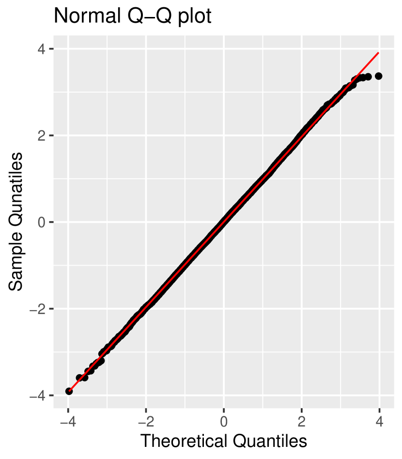
(a) DEGPD type (i)

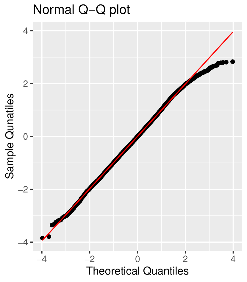
(b) DEGPD type (ii)

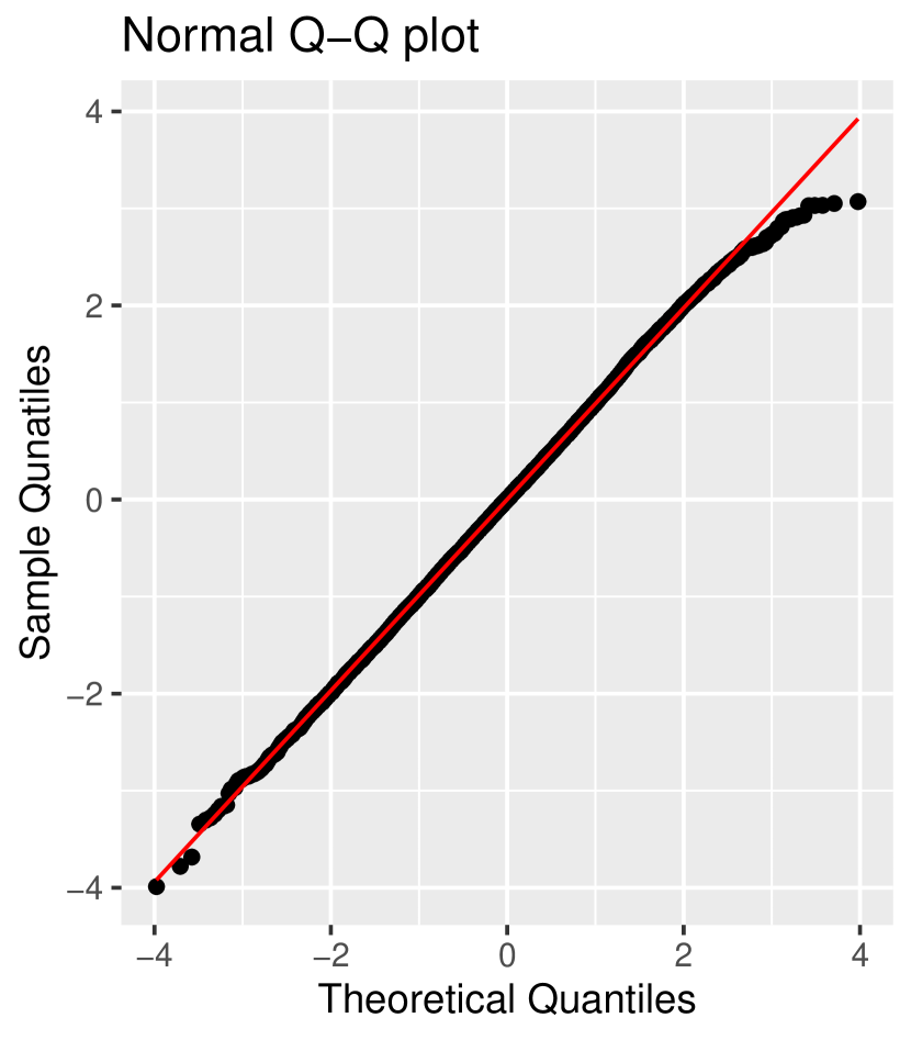
(c) DEGPD type (iii)

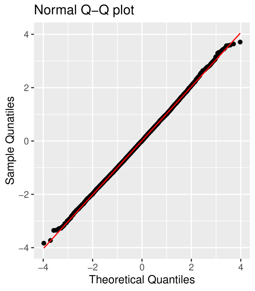
(d) DEGPD type (iv)

(e) DGPD

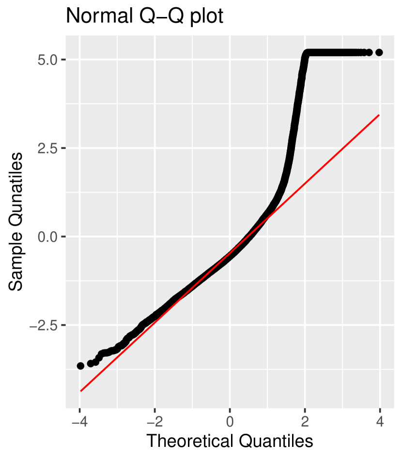
(f) Poisson

Figure 9: Diagnostic plots of residual quantiles of the proposed DEGPD type (i) to type (iv) and competitor (DGPD and Poisson) distributions.

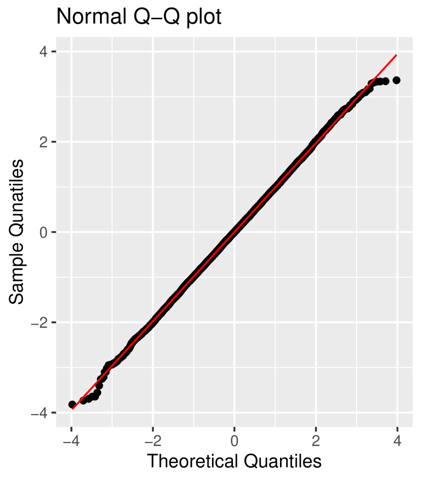
(a) ZIDEGPD type (i)

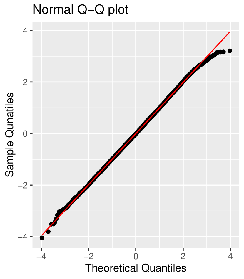
(b) ZIDEGPD type (ii)

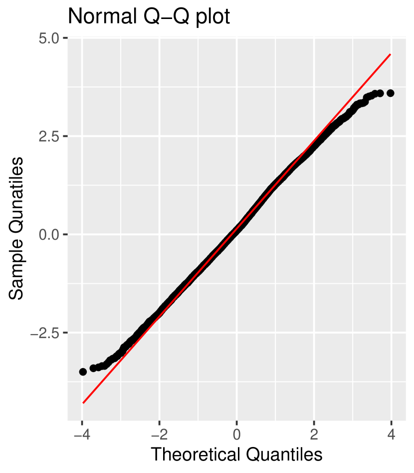
(c) ZIDEGPD type (iii)

Figure S2: Diagnostic plots of residual quantiles of the proposed ZIDEGPD type (i) to ZIDEGPD type (iii) models

The randomization allows to achieve continuous residuals even if the response variable is discrete. Aside from sampling variation in the parameter estimates, the randomized residuals appear to be exactly normal if the fitted model are correctly specified. Figure 9 shows normal quantile-quantile plots of randomized residuals of the proposed GAM form DEGPD type (i) to DEGPD type (iv) and competing models. Graphical representation of residuals of ZIDEGPD type (i) to ZIDEGPD type (iii) models is given in Figure S2 (see Supplementary material). The randomized residuals derived from on our proposed models show no apparent departure from normality detected, while randomized residuals based on DGPD and Poisson models departed from normality at the lower and upper tail, respectively.

We further check the normality of randomized residuals by using Kolmogorov–Smirnov test. Table 6 indicates that the newly proposed models considered for GAM form modeling deliver a good fit for the avalanches. among the different types, DEGPD type (i) and DEGPD type (iv) clearly outperforms the others as shown in Figure 9 as well. Furthermore, the randomized residuals from GPD and Poisson distribution not meet the normality assumption.

Table 6: Kolmogorov–Smirnov (KS) test statistics (p-values between parentheses) of the proposed DEGPD type (i) to type (iv) and competitor (DGPD and Poisson) distributions.

Model	DEGPD	DGPD	Poisson
(i)	0.0038 (0.9855)	0.0132 (0.0130)	0.21048 (2.2e-16)
(ii)	0.0106 (0.0779)
(iii)	0.0098 (0.1958)
(iv)	0.0066 (0.5590)

6 Conclusions

This study proposes different versions of DEGPD and ZIDEGPD models to demonstrate that it can jointly model the entire range of count data without selecting a threshold. Further, the DEGPD and ZIDEGPD GAM form models are developed and implemented. The flexibility of these models and their many practical advantages in discrete nature data make them very attractive. A few parameters make it simple to implement, interpret, and comply with discrete EVT for both upper and lower tails. The inference is performed through the MLE procedure, which shows more adequacy in results. Compared to ZIDEGPD, the fitted DEGPD appears more straightforward, robust, and genuinely represents zero proportion in the upheld complaints data of NYC. We observed that our proposed ZIDEGPD models are more flexible and robust for the data with zero inflation, and the remaining observations have rise in the lower tail up to structural mode and exponential decay at the upper heavier tail. As noted in the simulation study, the parameters $\delta$ and $\kappa_{2}$ gained more variability when estimated through the MLE method; Bayesian analysis with informative priors may improve the estimates of these parameters.

In addition, we developed and implemented the GAM forms methodology of our proposed models that allows for non-identically distributed discrete extremes. This methodology was implemented in evgam using the author’s written R functions. The response variable of interest (three day moving sum of daily avalanches at Haute-Maurienne massif of French Alps) is statistically explained by other environmental variables (e.g., temperature, wind, precipitation and humidity). GAM form models proposed in this study allows parametric non-parametric functional forms, which would most likely be required for larger datasets. Our models (espacially DEGPD and ZIDEGPD type (i)) also showing more flexibility and good fit for avalanches data with effect of environmental conditions as covariates than other competing models (i.e., DGPD, negative binomial and Poisson). It is worth to mentioned here that GAM form DEGPD models may perform more better to the other real data example. Again, GAM form ZIDEGPD models are more flexible and adequate when the response variable has a zero inflation, and the remaining observations have an exponential rise in the lower tail till mode and then decay at the upper heavier tail.

Hence, our proposed models can be applied to the variables which has discrete count data with extreme observation. Further, GAM forms proposals are flexible regarding spatial modelling of discrete extremes.

Code availability

The complete source code for the proposed models with simple running example is available on
https://github.com/touqeerahmadunipd/degpd-and-zidegpd

Supplementary material for
“Modelling of discrete extremes through extended versions of discrete generalized Pareto distribution”

1 The discrete Gamma spliced threshold discrete GPD model

As we have seen in existing literature, the discrete and continuous generalized Pareto limit distribution (GPD) is well approximated to the data which existing over a specified threshold. In continuous extreme value framework, many authors have tried to model the bulk part with some specific distribution (for example, Gamma, Normal, Log-normal, Weibull, and Beta distribution etc.). The arrangement, where data above and below an unknown threshold is drawn from the “bulk” and “tail” distributions respectively, meets into a family of models called spliced threshold models. The distinctive motivation for the model is the privilege that the data above and below the threshold are generated originally by two different underlying processes. For a thorough review of the general spliced threshold model in continuous domain (see, for example, Dey and Yan (2016)).

Let $F_{m}(x|\bm{\theta_{B}})$ is the CDF of gamma distribution which corresponds to bulk model and $F_{m}(x|\bm{\theta_{T}})$ is CDF of GPD corresponds to tail model, where $\bm{\theta}_{B}$ and $\bm{\theta}_{T}$ indicates the parameter vectors of bulk and tail models, respectively. The CDF of bulk and tail model spliced at threshold is given by

$$H_{m}(x)=\begin{cases}(1-\phi)\frac{F_{m}(x|\bm{\theta_{B}})}{F_{m}(u|\bm{\theta_{B}})}\hskip 56.9055ptfor\hskip 14.22636ptx\leq u\\ 1-\phi+\phi{F_{m}(x|\bm{\theta_{T}},u)}\hskip 28.45274ptfor\hskip 14.22636ptx>u\end{cases}$$ (S.1)

with corresponding probability density function

$$h_{m}(x)=\begin{cases}(1-\phi)\frac{f_{m}(x|\bm{\theta_{B}})}{F_{m}(u|\bm{\theta_{B}})}\hskip 56.9055ptfor\hskip 14.22636ptx\leq u\\ 1-\phi+\phi{f_{m}(x|\bm{\theta_{T}},u)}\hskip 28.45274ptfor\hskip 14.22636ptx>u\end{cases}$$ (S.2)

When we have discrete extreme data that characteristically exhibits several ties on the lower tail. That’s why, we need to amend the model developed before for continuous paradigm to discrete form in order to account the censored data. Let $X\sim Gamma(\alpha,\beta)$, we write the PMF of discrete gamma distribution as

$$P_{g}(X=k)=\frac{1}{\Gamma(\alpha)}\left[\gamma(\alpha,\beta(k+1))-\gamma(\alpha,\beta k\right]$$ (S.3)

where $\alpha>0,\beta>0$, $X\in\mathbb{N}$ and $\gamma(\alpha,\beta x)$ is the lower in complete gamma function

$$\gamma(\alpha,\beta k)=\int_{0}^{\beta k}t^{\alpha-1}e^{-t}dt$$ (S.4)

On the other hand, If $X\sim GPD(u,\sigma,\xi)$,the PMF of DGPD is written by using (4) as

$$P_{dp}(X=k)=\left(1+\frac{\xi(k-u)}{\sigma}\right)^{-1/\xi}-\left(1+\frac{\xi(k+1-u)}{\sigma}\right)^{-1/\xi}$$ (S.5)

for $(-\infty<u,\xi<\infty)$, $\sigma\in(0,\infty)$ and $k\in\mathbb{N}$. The DGPD support $k\geq u$ when $\xi\geq 0$ and $u\leq k\leq u-\frac{\sigma}{\xi}$ when $\xi<0$. Here, we may observe $\xi>0$. Hence, the discrete gamma generalized Pareto distribution (DGGPD) spliced at threshold model is given by

$$P_{d-ggp}(X=k)=\begin{cases}(1-\phi)\frac{P_{g}(X=k|\bm{\theta_{B})}}{F(u-d|\bm{\theta_{B}})}\hskip 56.9055ptfor\hskip 14.22636ptk\leq u-d\\ \phi P_{dp}(X=k|\bm{\theta_{T}},u)\hskip 56.9055ptfor\hskip 14.22636ptk\geq u\end{cases}$$ (S.6)

where $P_{g}(X=k|\bm{\theta_{B})}\sim$ discrete Gamma $(\alpha,\beta)$, $P_{dp}(X=k|\bm{\theta_{T})}\sim$ discrete GPD, $d=min(x)$, which indicates that we model integer data and $\phi$ is the proportion of observations over threshold $u$. For more details about mixture models and their implications (see e.g., Hu and Scarrott (2018)).

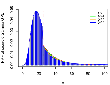
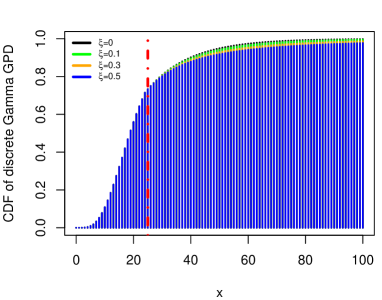
Figure S1: Probability mass function and the cumulative distribution function of discrete gamma GP spliced at threshold model corresponding to $\bm{\theta_{B}}=(\alpha=5,\beta=0.25)$, u=25, $\bm{\theta_{T}}=(\sigma=15,\xi=0,0.1,0.3,0.5)$

Figure S1 show the behavior of bulk and tail part in term of PMF and CDF of DGGPD spliced at threshold. Also, for fitting this mixture model suitable threshold is needed. However, to overcome this deficiency, the new framework to model whole range of data have been developed by avoiding the threshold selection issue.

2 Maximum likelihood procedure of DEGPD

(i) The PMF of DEGPD corresponding to $G(u;\psi)=u^{\kappa}$, $\psi=\kappa>0$ is written as

$$P(Y=k)=\left[\bigg{\{}1-\left(1+\frac{\xi(n+1)}{\sigma}\right)^{-\frac{1}{\xi}}\bigg{\}}^{\kappa}-\bigg{\{}1-\left(1+\frac{\xi n}{\sigma}\right)^{-\frac{1}{\xi}}\bigg{\}}^{\kappa}\right]$$ (S.7)

The log likelihood function is defined as

$$l(\kappa,\sigma,\xi)=\sum_{j=1}^{n}\log\left[\bigg{\{}1-\left(1+\frac{\xi(k_{j}+1)}{\sigma}\right)^{-\frac{1}{\xi}}\bigg{\}}^{\kappa}-\bigg{\{}1-\left(1+\frac{\xi(k_{j})}{\sigma}\right)^{-\frac{1}{\xi}}\bigg{\}}^{\kappa}\right]$$ (S.8)

(ii) First we need to define the PMF based on

$$G(u;\psi)=1-D_{\delta}\{(1-u)^{\delta}\},\hskip 28.45274pt\psi=\delta>0$$

where $D_{\delta}$ is CDF of beta distribution with parameters $1/\delta$ and 2. By definition

$$H(x)=G\left\{F_{\xi}\left(\frac{x}{\sigma}\right)\right\}$$

where $F_{\xi}(.)$ is the CDF of GPD. So,

$$H(x)=1-D_{\delta}\left[\left\{1-F_{\xi}\left(\frac{x}{\sigma}\right)\right\}^{\delta}\right]$$

$$H(x)=1-D_{\delta}\left[\left\{\bar{F}_{\xi}\left(\frac{x}{\sigma}\right)\right\}^{\delta}\right]$$ (S.9)

We solve, $D_{\delta}\left[\left\{\bar{F}_{\xi}\left(\frac{x}{\sigma}\right)\right\}^{\delta}\right]=D_{\delta}\left[z\right]$, where $z=\left\{\bar{F}_{\xi}\left(\frac{x}{\sigma}\right)\right\}^{\delta}$
The CDF of beta distribution with above specific parameters (i.e.,$1/\delta$ and 2) is written as

$$D_{\delta}(z,1/\delta,2)=\frac{B(z,1/\delta,2)}{B(1/\delta,2)}$$ (S.10)

After solving the Beta functions, we get

$$H(x)=1+\frac{1}{\delta}{\left[\bar{F}_{\xi}\left(\frac{x}{\sigma}\right)\right]}^{\delta+1}-\frac{\delta+1}{\delta}{\left[\bar{F}_{\xi}\left(\frac{x}{\sigma}\right)\right]}$$

The PMF of DEGPD corresponding to $G(u;\psi)=1-D_{\delta}\{(1-u)^{\delta}\}$ is written as

$$P(Y=k)=\frac{1}{\delta}{\left\{\left(1+\frac{\xi(k+1)}{\sigma}\right)^{-\frac{1}{\xi}}\right\}}^{\delta+1}-\frac{\delta+1}{\delta}{\left\{\left(1+\frac{\xi(k+1)}{\sigma}\right)^{-\frac{1}{\xi}}\right\}}\\ -\frac{1}{\delta}{\left\{\left(1+\frac{\xi k}{\sigma}\right)^{-\frac{1}{\xi}}\right\}}^{\delta+1}+\frac{\delta+1}{\delta}{\left\{\left(1+\frac{\xi k}{\sigma}\right)^{-\frac{1}{\xi}}\right\}}$$ (S.11)

The log likelihood function is defined as

$$l(\delta,\sigma,\xi)=\sum_{j=1}^{n}\log\Bigg{[}\frac{1}{\delta}{\left\{\left(1+\frac{\xi(k_{j}+1)}{\sigma}\right)^{-\frac{1}{\xi}}\right\}}^{\delta+1}-\frac{\delta+1}{\delta}{\left\{\left(1+\frac{\xi(k_{j}+1)}{\sigma}\right)^{-\frac{1}{\xi}}\right\}}\\ -\frac{1}{\delta}{\left\{\left(1+\frac{\xi k_{j}}{\sigma}\right)^{-\frac{1}{\xi}}\right\}}^{\delta+1}+\frac{\delta+1}{\delta}{\left\{\left(1+\frac{\xi k_{j}}{\sigma}\right)^{-\frac{1}{\xi}}\right\}}\Bigg{]}$$ (S.12)

(iii) Similar to model (ii), the CDF of EGPD corresponding to $G(u;\psi)=\left[1-D_{\delta}\{(1-u)^{\delta}\}\right]^{\kappa/2};\psi=(\delta,\kappa)>0$ is written as

$$H(x)=\left[F_{\xi}\left(\frac{x}{\sigma}\right)+\frac{1}{\delta}{\left[\bar{F}_{\xi}\left(\frac{x}{\sigma}\right)\right]}^{\delta+1}-\frac{1}{\delta}{\left[\bar{F}_{\xi}\left(\frac{x}{\sigma}\right)\right]}\right]^{\frac{\kappa}{2}}$$

The PMF of DEGPD corresponding to $G(u;\psi)=\left[1-D_{\delta}\{(1-u)^{\delta}\}\right]^{\kappa/2}$ can be written as

$$P(Y=k)=\left[1-\left(1+\frac{\xi(k+1)}{\sigma}\right)^{-\frac{1}{\xi}}+\frac{1}{\delta}{\left\{\left(1+\frac{\xi(k+1)}{\sigma}\right)^{-\frac{1}{\xi}}\right\}}^{\delta+1}-\frac{1}{\delta}{\left\{\left(1+\frac{\xi(k+1)}{\sigma}\right)^{-\frac{1}{\xi}}\right\}}\right]^{\frac{\kappa}{2}}\\ -\left[1-\left(1+\frac{\xi k}{\sigma}\right)^{-\frac{1}{\xi}}+\frac{1}{\delta}{\left\{\left(1+\frac{\xi k}{\sigma}\right)^{-\frac{1}{\xi}}\right\}}^{\delta+1}-\frac{1}{\delta}{\left\{\left(1+\frac{\xi k}{\sigma}\right)^{-\frac{1}{\xi}}\right\}}\right]^{\frac{\kappa}{2}}$$ (S.13)

The log likelihood function is defined as

$$l(\kappa,\delta,\sigma,\xi)=\sum_{j=1}^{n}\log\Bigg{[}\Bigg{[}1-\left(1+\frac{\xi(k_{j}+1)}{\sigma}\right)^{-\frac{1}{\xi}}+\frac{1}{\delta}{\left\{\left(1+\frac{\xi(k_{j}+1)}{\sigma}\right)^{-\frac{1}{\xi}}\right\}}^{\delta+1}\\ -\frac{1}{\delta}{\left\{\left(1+\frac{\xi(k_{j}+1)}{\sigma}\right)^{-\frac{1}{\xi}}\right\}}\Bigg{]}^{\frac{\kappa}{2}}-\Bigg{[}1-\left(1+\frac{\xi k_{j}}{\sigma}\right)^{-\frac{1}{\xi}}+\frac{1}{\delta}{\left\{\left(1+\frac{\xi k_{j}}{\sigma}\right)^{-\frac{1}{\xi}}\right\}}^{\delta+1}\\ -\frac{1}{\delta}{\left\{\left(1+\frac{\xi k_{j}}{\sigma}\right)^{-\frac{1}{\xi}}\right\}}\Bigg{]}^{\frac{\kappa}{2}}\Bigg{]}$$ (S.14)

(iv) The PMF corresponding to $G(u;\psi)=pu^{\kappa_{1}}+(1-p)u^{\kappa_{2}}$, $\psi=(p,\kappa_{1},\kappa_{2})>0$ with $\kappa_{1}\leq\kappa_{2}$ is written as

$$P(Y=k)=p\left[\left\{1-\left(1+\frac{\xi(k+1)}{\sigma}\right)^{-\frac{1}{\xi}}\right\}^{\kappa_{1}}-\left\{1-\left(1+\frac{\xi k}{\sigma}\right)^{-\frac{1}{\xi}}\right\}^{\kappa_{1}}\right]\\ +(1-p)\left[\left\{1-\left(1+\frac{\xi(k+1)}{\sigma}\right)^{-\frac{1}{\xi}}\right\}^{\kappa_{2}}-\left\{1-\left(1+\frac{\xi k}{\sigma}\right)^{-\frac{1}{\xi}}\right\}^{\kappa_{2}}\right]$$ (S.15)

The likelihood function is defined as

$$l(p,\kappa_{1},\kappa_{2},\sigma,\xi)=\sum_{j=1}^{n}\log\Bigg{[}p\left[\left\{1-\left(1+\frac{\xi(k_{j}+1)}{\sigma}\right)^{-\frac{1}{\xi}}\right\}^{\kappa_{1}}-\left\{1-\left(1+\frac{\xi k_{j}}{\sigma}\right)^{-\frac{1}{\xi}}\right\}^{\kappa_{1}}\right]\\ +(1-p)\left[\left\{1-\left(1+\frac{\xi(k_{j}+1)}{\sigma}\right)^{-\frac{1}{\xi}}\right\}^{\kappa_{2}}-\left\{1-\left(1+\frac{\xi k_{j}}{\sigma}\right)^{-\frac{1}{\xi}}\right\}^{\kappa_{2}}\right]\Bigg{]}$$ (S.16)

To find the estimates of unknown parameters of above model, we solve the derivatives of log likelihood function of model (i), (ii), (iii) and (iv) numerically.

3 Maximum likelihood procedure of ZIDEGPD

(i) The PMF of ZIDEGPD based on $G(u;\psi)=u^{\kappa}$, $\psi=\kappa>0$ is written as

$$P(Z=m)=\begin{cases}\pi+(1-\pi)\left[1-\left(1+\frac{\xi}{\sigma}\right)^{-\frac{1}{\xi}}\right]^{\kappa},\hskip 142.26378ptm=0\\ (1-\pi)\left[\bigg{\{}1-\left(1+\frac{\xi(m+1)}{\sigma}\right)^{-\frac{1}{\xi}}\bigg{\}}^{\kappa}-\bigg{\{}1-\left(1+\frac{\xi(m)}{\sigma}\right)^{-\frac{1}{\xi}}\bigg{\}}^{\kappa}\right],\hskip 14.22636ptm>0\end{cases}$$ (S.17)

Thus, the likelihood function is defined as

$$L(\theta)=\left[\pi+(1-\pi)G\left\{F_{\xi}\left(\frac{1}{\sigma}\right)\right\}\right]^{r}\prod_{{j=1};m_{j}\neq 0}^{n}(1-\pi)\left[G\left\{F_{\xi}\left(\frac{m_{j}+1}{\sigma}\right)\right\}-G\left\{F_{\xi}\left(\frac{m_{j}}{\sigma}\right)\right\}\right]$$ (S.18)

The log likelihood function is

$$l(\pi,\kappa,\sigma,\xi)=r\log\left[\pi+(1-\pi)\left\{1-\left(1+\frac{\xi}{\sigma}\right)^{-\frac{1}{\xi}}\right\}^{\kappa}\right]+(n-r)\log(1-\pi)\\ +\sum_{j=1}^{n}\log\left[\bigg{\{}1-\left(1+\frac{\xi(m_{j}+1)}{\sigma}\right)^{-\frac{1}{\xi}}\bigg{\}}^{\kappa}-\bigg{\{}1-\left(1+\frac{\xi(m_{j})}{\sigma}\right)^{-\frac{1}{\xi}}\bigg{\}}^{\kappa}\right]$$ (S.19)

(ii) The PMF of ZIDEGPD obtained via $G(u;\psi)=1-D_{\delta}\{(1-u)^{\delta}\},\hskip 28.45274pt\psi=\delta>0$

$$P(Z=m)=\begin{cases}\pi+(1-\pi)\left[\frac{1}{\delta}{\left\{\left(1+\frac{\xi}{\sigma}\right)^{-\frac{1}{\xi}}\right\}}^{\delta+1}-\frac{\delta+1}{\delta}{\left\{\left(1+\frac{\xi}{\sigma}\right)^{-\frac{1}{\xi}}\right\}}+1\right],\hskip 14.22636ptm=0\\ (1-\pi)\Bigg{[}\frac{1}{\delta}{\left\{\left(1+\frac{\xi(m+1)}{\sigma}\right)^{-\frac{1}{\xi}}\right\}}^{\delta+1}-\frac{\delta+1}{\delta}{\left\{\left(1+\frac{\xi(m+1)}{\sigma}\right)^{-\frac{1}{\xi}}\right\}}\\ -\frac{1}{\delta}{\left\{\left(1+\frac{\xi m}{\sigma}\right)^{-\frac{1}{\xi}}\right\}}^{\delta+1}+\frac{\delta+1}{\delta}{\left\{\left(1+\frac{\xi m}{\sigma}\right)^{-\frac{1}{\xi}}\right\}}\Bigg{]},\hskip 85.35826ptm>0\end{cases}$$ (S.20)

The log likelihood function is defined as

$$l(\pi,\delta,\sigma,\xi)=r\log\left[\pi+(1-\pi)\left[\frac{1}{\delta}{\left\{\left(1+\frac{\xi}{\sigma}\right)^{-\frac{1}{\xi}}\right\}}^{\delta+1}-\frac{\delta+1}{\delta}{\left\{\left(1+\frac{\xi}{\sigma}\right)^{-\frac{1}{\xi}}\right\}}+1\right]\right]\\ +(n-r)\log(1-\pi)+\sum_{j=1}^{n}\log\Bigg{[}\frac{1}{\delta}{\left\{\left(1+\frac{\xi(m_{j}+1)}{\sigma}\right)^{-\frac{1}{\xi}}\right\}}^{\delta+1}\\ -\frac{\delta+1}{\delta}{\left\{\left(1+\frac{\xi(m_{j}+1)}{\sigma}\right)^{-\frac{1}{\xi}}\right\}}-\frac{1}{\delta}{\left\{\left(1+\frac{\xi m_{j}}{\sigma}\right)^{-\frac{1}{\xi}}\right\}}^{\delta+1}+\frac{\delta+1}{\delta}{\left\{\left(1+\frac{\xi m_{j}}{\sigma}\right)^{-\frac{1}{\xi}}\right\}}\Bigg{]}$$ (S.21)

(iii) The PMF of ZIDEGPD corresponding to $G(u;\psi)=\left[1-D_{\delta}\{(1-u)^{\delta}\}\right]^{\kappa/2};\psi=(\delta,\kappa)>0$ is

$$P(Z=m)=\begin{cases}\pi+(1-\pi)\left[\left[1-\left(1+\frac{\xi}{\sigma}\right)^{-\frac{1}{\xi}}+\frac{1}{\delta}{\left\{\left(1+\frac{\xi}{\sigma}\right)^{-\frac{1}{\xi}}\right\}}^{\delta+1}-\frac{1}{\delta}{\left\{\left(1+\frac{\xi}{\sigma}\right)^{-\frac{1}{\xi}}\right\}}\right]^{\frac{\kappa}{2}}\right],\hskip 5.69046ptm=0\\ (1-\pi)\Bigg{[}\left[1-\left(1+\frac{\xi(m+1)}{\sigma}\right)^{-\frac{1}{\xi}}+\frac{1}{\delta}{\left\{\left(1+\frac{\xi(m+1)}{\sigma}\right)^{-\frac{1}{\xi}}\right\}}^{\delta+1}-\frac{1}{\delta}{\left\{\left(1+\frac{\xi(m+1)}{\sigma}\right)^{-\frac{1}{\xi}}\right\}}\right]^{\frac{\kappa}{2}}\\ -\left[1-\left(1+\frac{\xi m}{\sigma}\right)^{-\frac{1}{\xi}}+\frac{1}{\delta}{\left\{\left(1+\frac{\xi m}{\sigma}\right)^{-\frac{1}{\xi}}\right\}}^{\delta+1}-\frac{1}{\delta}{\left\{\left(1+\frac{\xi m}{\sigma}\right)^{-\frac{1}{\xi}}\right\}}\right]^{\frac{\kappa}{2}}\Bigg{]},\hskip 28.45274ptm>0\end{cases}$$ (S.22)

The log likelihood function is defined as

$$l(\pi,\kappa,\delta,\sigma,\xi)=r\log\Bigg{[}\pi+(1-\pi)\left[\left[1-\left(1+\frac{\xi}{\sigma}\right)^{-\frac{1}{\xi}}+\frac{1}{\delta}{\left\{\left(1+\frac{\xi}{\sigma}\right)^{-\frac{1}{\xi}}\right\}}^{\delta+1}-\frac{1}{\delta}{\left\{\left(1+\frac{\xi}{\sigma}\right)^{-\frac{1}{\xi}}\right\}}\right]^{\frac{\kappa}{2}}\right]\Bigg{]}\\ +(n-r)\log(1-\pi)+\sum_{j=1}^{n}\log\Bigg{[}\Bigg{[}1-\left(1+\frac{\xi(m_{j}+1)}{\sigma}\right)^{-\frac{1}{\xi}}\\ +\frac{1}{\delta}{\left\{\left(1+\frac{\xi(m_{j}+1)}{\sigma}\right)^{-\frac{1}{\xi}}\right\}}^{\delta+1}-\frac{1}{\delta}{\left\{\left(1+\frac{\xi(m_{j}+1)}{\sigma}\right)^{-\frac{1}{\xi}}\right\}}\Bigg{]}^{\frac{\kappa}{2}}-\\ \Bigg{[}1-\left(1+\frac{\xi m_{j}}{\sigma}\right)^{-\frac{1}{\xi}}+\frac{1}{\delta}{\left\{\left(1+\frac{\xi m_{j}}{\sigma}\right)^{-\frac{1}{\xi}}\right\}}^{\delta+1}-\frac{1}{\delta}{\left\{\left(1+\frac{\xi m_{j}}{\sigma}\right)^{-\frac{1}{\xi}}\right\}}\Bigg{]}^{\frac{\kappa}{2}}\Bigg{]}$$ (S.23)

(iv) The PMF of ZIDGPD corresponding to $G(u;\psi)=pu^{\kappa_{1}}+(1-p)u^{\kappa_{2}}$, $\psi=(p,\kappa_{1},\kappa_{2})>0$ is

$$P(Z=m)=\begin{cases}\pi+(1-\pi)\left[p\left\{1-\left(1+\frac{\xi}{\sigma}\right)^{-\frac{1}{\xi}}\right\}^{\kappa_{1}}+(1-p)\left[\left\{1-\left(1+\frac{\xi}{\sigma}\right)^{-\frac{1}{\xi}}\right\}^{\kappa_{2}}\right]\right],\hskip 5.69046ptm=0\\ (1-\pi)\Bigg{[}p\left[\left\{1-\left(1+\frac{\xi(m+1)}{\sigma}\right)^{-\frac{1}{\xi}}\right\}^{\kappa_{1}}-\left\{1-\left(1+\frac{\xi m}{\sigma}\right)^{-\frac{1}{\xi}}\right\}^{\kappa_{1}}\right]\\ +(1-p)\left[\left\{1-\left(1+\frac{\xi(m+1)}{\sigma}\right)^{-\frac{1}{\xi}}\right\}^{\kappa_{2}}-\left\{1-\left(1+\frac{\xi m}{\sigma}\right)^{-\frac{1}{\xi}}\right\}^{\kappa_{2}}\right]\Bigg{]},\hskip 28.45274ptx>0\end{cases}$$ (S.24)

The likelihood function is defined as

$$l(\pi,p,\kappa_{1},\kappa_{2},\sigma,\xi)=r\log\Bigg{[}\pi+(1-\pi)\left[p\left\{1-\left(1+\frac{\xi}{\sigma}\right)^{-\frac{1}{\xi}}\right\}^{\kappa_{1}}+(1-p)\left[\left\{1-\left(1+\frac{\xi}{\sigma}\right)^{-\frac{1}{\xi}}\right\}^{\kappa_{2}}\right]\right]\Bigg{]}\\ +(n-r)\log(1-\pi)+\sum_{j=1}^{n}\log\Bigg{[}p\left[\left\{1-\left(1+\frac{\xi(m_{j}+1)}{\sigma}\right)^{-\frac{1}{\xi}}\right\}^{\kappa_{1}}-\left\{1-\left(1+\frac{\xi m_{j}}{\sigma}\right)^{-\frac{1}{\xi}}\right\}^{\kappa_{1}}\right]\\ +(1-p)\left[\left\{1-\left(1+\frac{\xi(m_{j}+1)}{\sigma}\right)^{-\frac{1}{\xi}}\right\}^{\kappa_{2}}-\left\{1-\left(1+\frac{\xi m_{j}}{\sigma}\right)^{-\frac{1}{\xi}}\right\}^{\kappa_{2}}\right]\Bigg{]}$$ (S.25)

Similar to DEGPD, the unknown parameters of ZIDEGPD models, we solve the derivatives of log likelihood function of model (i), (ii), (iii) and (iv) numerically.

Table S1: Root mean square errors of parameter estimates ZIDEGPD found from $10^{4}$ independent data sets of size $n=1000$.

Model type (i) $G(u;\psi)=u^{\kappa}$
$\pi$		$\kappa$		$\sigma$		$\xi$		$-$		$-$
TRUE	RMSE	TRUE	RMSE	TRUE	RMSE	TRUE	RMSE	TRUE	RMSE	TRUE	RMSE
0.2	0.04	5	3.00	1	0.28	0.2	0.06
0.2	0.01	10	3.19	1	0.20	0.2	0.04
0.5	0.03	5	3.83	1	0.34	0.2	0.07
0.5	0.02	10	3.97	1	0.25	0.2	0.05
Model type (ii) $G(u;\psi)=1-D_{\delta}\{(1-u)^{\delta}\}$
$\pi$		$\delta$		$\sigma$		$\xi$		$-$		$-$
0.2	0.09	1	4.18	1	0.22	0.20	0.06
0.2	0.10	5	3.08	1	0.17	0.20	0.06
0.5	0.06	1	4.10	1	0.20	0.20	0.07
0.5	0.09	5	1.72	1	0.20	0.20	0.08
Model type (iii) $G(u;\psi)=\left[1-D_{\delta}\{(1-u)^{\delta}\}\right]^{\kappa/2}$
$\pi$		$\kappa$		$\delta$		$\sigma$		$\xi$		$-$
0.2	0.03	5	6.09	1	1.90	1	0.29	0.20	0.05
0.2	0.02	10	4.20	5	4.10	1	0.27	0.20	0.05
0.5	0.03	5	4.49	1	1.63	1	0.38	0.20	0.07
0.5	0.02	10	5.41	5	4.80	1	0.34	0.20	0.07
Model type (iv) $G(u;\psi)=pu^{\kappa_{1}}+(1-p)u^{\kappa_{2}}$
$\pi$		$p$		$\kappa_{1}$		$\kappa_{2}$		$\sigma$		$\xi$
0.2	0.14	0.5	0.29	1	4.03	5	4.16	1	0.34	0.20	0.07
0.2	0.07	0.5	0.30	5	2.24	10	9.40	1	0.25	0.20	0.05
0.5	0.23	0.5	0.35	1	0.66	5	2.14	1	0.37	0.20	0.08
0.5	0.09	0.5	0.33	5	2.33	10	7.64	1	0.27	0.2	0.06

Table S2: Estimated coefficients and smooth terms for GAM form ZIDEGPD models fitted to Avalanches data of Haute-Maurienne massif of French Alps

Model type (i) $G(u;\psi)=u^{\kappa}$
** Parametric terms **
Parameter (intercept)	Estimate	Std.Error	t value	P-value
$\log(\kappa)$	-1.83	0.06	-32.25	$<$2e-16
$\log(\sigma)$	0.2	0.1	1.99	0.0232
$\log(\xi)$	-0.53	0.08	-6.84	4.04e-12
$logit(\pi)$	-52.06	0.09	-16.84	6.02e-13
** Smooth terms **
$\log(\sigma)$	edf	max.df	Chi.sq	Pr($>|t|$)
s(WS)	1.02	4	23.56	1.29e-06
s(MxT)	3.99	4	652.73	$<$2e-16
s(PREC)	1.00	4	36.41	1.6e-09
s(RH)	4.19	9	70.35	7.59e-14
Model type (ii) $G(u;\psi)=1-F_{\delta}\{(1-u)^{\delta}\}$
** Parametric terms **
Parameter (intercept)	Estimate	Std.Error	t value	P-value
$\log(\delta)$	4.67	599.22	0.01	0.497
$\log(\sigma)$	-0.73	0.08	-8.92	$<$2e-16
$\log(\xi)$	-0.3	0.05	-6.17	3.44e-10
$logit(\pi)$	0.48	9.04	0.05	0.479
** Smooth terms **
$\log(\sigma)$
s(WS)	1.71	4	22.34	1.3e-05
s(MxT)	2.54	4	692.76	$<$2e-16
s(PREC)	1.03	4	33.96	7.51e-09
s(RH)	5.50	9	85.89	3.46e-16
Model type (iii) $G(u;\psi)=\left[1-F_{\delta}\{(1-u)^{\delta}\}\right]^{\kappa/2}$
** Parametric terms **
Parameter (intercept)	Estimate	Std.Error	t value	P-value
$\log(\kappa)$	-1.23	0.21	-5.96	1.27e-09
$\log(\delta)$	2.1	0.43	4.86	5.83e-07
$\log(\sigma)$	0.52	0.01	37.92	$<$2e-16
$\log(\xi)$	-0.65	0.07	-9.43	$<$2e-16
$logit(\pi)$	-0.96	0.59	-1.62	0.0528
** Smooth terms **
$\log(\sigma)$
s(WS)	1.00	4	610.20	$<$2e-16
s(MxT)	3.95	4	11340.79	$<$2e-16
s(PREC)	1.01	4	792.57	$<$2e-16
s(RH)	7.89	9	1701.40	$<$2e-16

References

- (1)
- Beirlant et al. (2004) Beirlant, J., Goegebeur, Y., Segers, J., and Teugels, J. L. (2004), Statistics of Extremes: Theory and Applications, New York: John Wiley & Sons.
- Boutsikas and Koutras (2002) Boutsikas, M., and Koutras, M. (2002), “Modeling claim exceedances over thresholds,” Insurance: Mathematics and Economics, 30(1), 67–83.
- Buddana and Kozubowski (2014) Buddana, A., and Kozubowski, T. J. (2014), “Discrete Pareto distributions,” Economic Quality Control, 29(2), 143–156.
- Carreau and Bengio (2009) Carreau, J., and Bengio, Y. (2009), “A hybrid Pareto model for asymmetric fat-tailed data: the univariate case,” Extremes, 12(1), 53–76.
- Carrer and Gaetan (2022) Carrer, N. L., and Gaetan, C. (2022), “Distributional regression models for Extended Generalized Pareto distributions,” arXiv preprint arXiv:2209.04660, .
- Chavez-Demoulin and Davison (2005) Chavez-Demoulin, V., and Davison, A. C. (2005), “Generalized additive modelling of sample extremes,” Journal of the Royal Statistical Society: Series C (Applied Statistics), 54(1), 207–222.
- Chiogna and Gaetan (2007) Chiogna, M., and Gaetan, C. (2007), “Semiparametric zero-inflated Poisson models with application to animal abundance studies,” Environmetrics, 18(3), 303–314.
- Choulakian and Stephens (2001) Choulakian, V., and Stephens, M. A. (2001), “Goodness-of-fit tests for the generalized Pareto distribution,” Technometrics, 43(4), 478–484.
- Coles (2001) Coles, S. (2001), An Introduction to Statistical Modeling of Extreme Values, New York: Springer.
- Davison and Smith (1990) Davison, A. C., and Smith, R. L. (1990), “Models for exceedances over high thresholds,” Journal of the Royal Statistical Society: Series B (Methodological), 52(3), 393–425.
- de Carvalho et al. (2022) de Carvalho, M., Pereira, S., Pereira, P., and de Zea Bermudez, P. (2022), “An Extreme Value Bayesian Lasso for the Conditional Left and Right Tails,” Journal of Agricultural, Biological and Environmental Statistics, 27, 222–239.
- de Hann and Ferreira (2006) de Hann, L., and Ferreira, A. (2006), Extreme Value Theory: an Introduction, New York: Springer.
- Dey and Yan (2016) Dey, D. K., and Yan, J. (2016), Extreme Value Modeling and Risk analysis: Methods and Applications, New York: CRC Press.
- Dkengne et al. (2016) Dkengne, P. S., Eckert, N., and Naveau, P. (2016), “A limiting distribution for maxima of discrete stationary triangular arrays with an application to risk due to avalanches,” Extremes, 19(1), 25–40.
- Dunn and Smyth (1996) Dunn, P. K., and Smyth, G. K. (1996), “Randomized quantile residuals,” Journal of Computational and graphical statistics, 5(3), 236–244.
- Dupuis (1999) Dupuis, D. J. (1999), “Exceedances over high thresholds: A guide to threshold selection,” Extremes, 1(3), 251–261.
- Embrechts et al. (1999) Embrechts, P., Kluppelberg, C., and Mikosch, T. (1999), “Modelling extremal events,” British actuarial journal, 5(2), 465–465.
- Evin et al. (2021) Evin, G., Sielenou, P. D., Eckert, N., Naveau, P., Hagenmuller, P., and Morin, S. (2021), “Extreme avalanche cycles: Return levels and probability distributions depending on snow and meteorological conditions,” Weather and Climate Extremes, 33, 100344.
- Fisher and Tippett (1928) Fisher, R. A., and Tippett, L. H. C. (1928), Limiting forms of the frequency distribution of the largest or smallest member of a sample,, in Mathematical Proceedings of the Cambridge philosophical society, Vol. 24, Cambridge University Press, pp. 180–190.
- Frigessi et al. (2002) Frigessi, A., Haug, O., and Rue, H. (2002), “A dynamic mixture model for unsupervised tail estimation without threshold selection,” Extremes, 5(3), 219–235.
- Furrer and Naveau (2007) Furrer, R., and Naveau, P. (2007), “Probability weighted moments properties for small samples,” Statistics and Probability Letters, 77, 190–195.
- Gamet and Jalbert (2022) Gamet, P., and Jalbert, J. (2022), “A flexible extended generalized Pareto distribution for tail estimation,” Environmetrics, 33(6), e2744.
- Hastie and Tibshirani (1990) Hastie, T., and Tibshirani, R. (1990), Generalized Additive Models, New York: Chapman & Hall, CRC Press.
- Hitz et al. (2017) Hitz, A., Davis, R., and Samorodnitsky, G. (2017), “Discrete extremes,” arXiv preprint arXiv:1707.05033, .
- Hu and Scarrott (2018) Hu, Y., and Scarrott, C. (2018), “evmix: An R package for extreme value mixture modeling, threshold estimation and boundary corrected kernel density estimation,” , .
- Katz et al. (2002) Katz, R. W., Parlange, M. B., and Naveau, P. (2002), “Statistics of extremes in hydrology,” Advances in water resources, 25(8-12), 1287–1304.
- Kozubowski et al. (2015) Kozubowski, T. J., Panorska, A. K., and Forister, M. L. (2015), “A discrete truncated Pareto distribution,” Statistical Methodology, 26, 135–150.
- Krishna and Pundir (2009) Krishna, H., and Pundir, P. S. (2009), “Discrete Burr and discrete Pareto distributions,” Statistical Methodology, 6(2), 177–188.
- Lambert (1992) Lambert, D. (1992), “Zero-inflated Poisson regression, with an application to defects in manufacturing,” Technometrics, 34(1), 1–14.
- Le Gall et al. (2022) Le Gall, P., Favre, A.-C., Naveau, P., and Prieur, C. (2022), “Improved regional frequency analysis of rainfall data,” Weather and Climate Extremes, 36, 100456.
- MacDonald et al. (2011) MacDonald, A., Scarrott, C. J., Lee, D., Darlow, B., Reale, M., and Russell, G. (2011), “A flexible extreme value mixture model,” Computational Statistics & Data Analysis, 55(6), 2137–2157.
- Mougin (1922) Mougin, P. (1922), “Avalanches in Savoy, vol. IV,” Ministry of Agriculture, General Directorate of Water and Forests, Department of Great Hydraulic Forces, Paris, .
- Naveau et al. (2016) Naveau, P., Huser, R., Ribereau, P., and Hannart, A. (2016), “Modeling jointly low, moderate, and heavy rainfall intensities without a threshold selection,” Water Resources Research, 52(4), 2753–2769.
- Pauli and Coles (2001) Pauli, F., and Coles, S. (2001), “Penalized likelihood inference in extreme value analyses,” Journal of Applied Statistics, 28(5), 547–560.
- Pickands (1975) Pickands, J. (1975), “Statistical inference using extreme order statistics,” the Annals of Statistics, pp. 119–131.
- Prieto et al. (2014) Prieto, F., Gómez-Déniz, E., and Sarabia, J. M. (2014), “Modelling road accident blackspots data with the discrete generalized Pareto distribution,” Accident Analysis & Prevention, 71, 38–49.
- Ranjbar et al. (2022) Ranjbar, S., Cantoni, E., Chavez-Demoulin, V., Marra, G., Radice, R., and Jaton, K. (2022), “Modelling the extremes of seasonal viruses and hospital congestion: The example of flu in a Swiss hospital,” Journal of the Royal Statistical Society: Series C (Applied Statistics), 71(4), 884–905.
- Ribereau et al. (2016) Ribereau, P., Masiello, E., and Naveau, P. (2016), “Skew generalized extreme value distribution: Probability-weighted moments estimation and application to block maxima procedure,” Communications in Statistics-Theory and Methods, 45(17), 5037–5052.
- Rigby and Stasinopoulos (2005) Rigby, R. A., and Stasinopoulos, D. M. (2005), “Generalized additive models for location, scale and shape,” Journal of the Royal Statistical Society: Series C (Applied Statistics), 54(3), 507–554.
- Sartori (2006) Sartori, N. (2006), “Bias prevention of maximum likelihood estimates for scalar skew normal and skew t distributions,” Journal of Statistical Planning and Inference, 136(12), 4259–4275.
- Scarrott and MacDonald (2012) Scarrott, C., and MacDonald, A. (2012), “A review of extreme value threshold estimation and uncertainty quantification,” REVSTAT–Statistical Journal, 10(1), 33–60.
- Stasinopoulos et al. (2018) Stasinopoulos, M. D., Rigby, R. A., and Bastiani, F. D. (2018), “GAMLSS: A distributional regression approach,” Statistical Modelling, 18, 248–273.
- Tencaliec et al. (2019) Tencaliec, P., Favre, A., Naveau, P., Prieur, C., and Nicolet, G. (2019), “Flexible semiparametric generalized Pareto modeling of the entire range of rainfall amount,” Environmetrics, env.2582.
- Wood (2017) Wood, S. N. (2017), Generalized Additive models: an Introduction with R, 2nd edn, New York: Chapman and Hall/CRC.
- Yee and Stephenson (2007) Yee, T. W., and Stephenson, A. G. (2007), “Vector generalized linear and additive extreme value models,” Extremes, 10(1), 1–19.
- Youngman (2019) Youngman, B. D. (2019), “Generalized additive models for exceedances of high thresholds with an application to return level estimation for US wind gusts,” Journal of the American Statistical Association, 114(528), 1865–1879.
- Youngman (2020) Youngman, B. D. (2020), “evgam: an R package for generalized additive extreme value models,” arXiv preprint:2003.04067, .