Spoofing cross entropy measure in boson sampling
Abstract
Cross entropy (XE) measure is a widely used benchmarking to demonstrate quantum computational advantage from sampling problems, such as random circuit sampling using superconducting qubits and boson sampling (BS). We present a heuristic classical algorithm that attains a better XE than the current BS experiments in a verifiable regime and is likely to attain a better XE score than the near-future BS experiments in a reasonable running time. The key idea behind the algorithm is that there exist distributions that correlate with the ideal BS probability distribution and that can be efficiently computed. The correlation and the computability of the distribution enable us to post-select heavy outcomes of the ideal probability distribution without computing the ideal probability, which essentially leads to a large XE. Our method scores a better XE than the recent Gaussian BS experiments when implemented at intermediate, verifiable system sizes. Much like current state-of-the-art experiments, we cannot verify that our spoofer works for quantum advantage size systems. However, we demonstrate that our approach works for much larger system sizes in fermion sampling, where we can efficiently compute output probabilities. Finally, we provide analytic evidence that the classical algorithm is likely to spoof noisy BS efficiently.
Quantum computers are believed to efficiently solve problems that classical counterparts cannot, such as integer factoring [1] and quantum simulation [2]. Whereas scalability and fault tolerance are required to solve hard and practical problems, currently available devices are noisy intermediate-scale quantum (NISQ). Hence, huge attention has been paid to demonstrating quantum advantage by exploiting NISQ devices. Sampling problems are particularly promising for the demonstration thanks to rigorous evidence that classical computers cannot efficiently solve them [3, 4, 5, 6]. Indeed, we have recently seen the first claims of quantum advantage using random circuit sampling (RCS) with superconducting qubits [7, 8, 9] and Gaussian boson sampling (GBS) [10, 11, 12, 13]. However, the apparent limitation of current experiments is that they are not scalable because uncorrected noise decays quantum signal as the system size grows [14, 15, 16, 17, 18, 19, 20, 21, 22, 23, 24, 25, 26, 27, 28, 29]. Thus, finding appropriate size experiments is crucial in which the system size is sufficiently large so that classical computers cannot efficiently simulate them but not too large for noise to annihilate quantum signals.
Finding an appropriate regime is also important to enable classical verification because verification techniques such as cross-entropy benchmarking (XEB) cost exponential time [30]. The state-of-the-art method is XEB, which is sample-efficient for RCS and GBS 111XEB is sample-efficient in the sense that it does not require an exponentially large number of samples while it is computationally inefficient because computing the ideal output probability requires exponential time.; scoring a large XE is considered evidence of quantum advantage. The premise behind the benchmarking is that appropriate-size experiments maintain sufficient quantum signals so that the experimental score cannot be attained by classical devices within reasonable costs due to the remaining quantum signals. For RCS [7, 8], there have been extensive studies to support the premise [30, 7, 32, 33]. While we have some limited understanding of what XE measures in RCS [34, 30, 7, 32, 33, 35] with many interesting debates of XEB [35, 34], our understanding of XE in BS is much more limited than RCS. Crucially, there is no theoretical evidence that attaining a high XE is classically hard, to the best of our knowledge. Despite this, the XEB has been used in many state-of-the-art quantum advantage experiments [10, 11, 12, 13]. XEB is particularly attractive since the benchmark does not depend on an adversarial mock-up distribution. This adversary independence feature allows us to use XEB to benchmark noisy experiments in situations in which we are ignorant of the best possible classical spoofing algorithm, as is the case with GBS experiments 222Other benchmarking methods employed [10, 11, 12, 13], such as Bayesian test and correlator methods, also do not have rigorous evidence for hardness. Also, the Bayesian test is genuinely implemented against adversarial samplers; thus, it cannot rule out all possible classical algorithms. We emphasize that the current GBS experiments employ XEB against certain adversarial samplers because we do not know the ideal score..
In this Letter, we provide a heuristic classical algorithm that scores better than the current intermediate-scale GBS (in a verifiable regime) and is likely to score better than the near-future BS experiments for XEB. First, we numerically demonstrate using a small-scale GBS that our algorithm selectively generates heavy outcomes of BS and scores better than the ideal distribution. For larger systems in a quantum advantage regime, due to the inefficiency of estimating XE and a large computational cost, the frequently used method is to analyze an intermediate-size experiment in a classically verifiable regime, instead of the largest experiment. Following this, we demonstrate that the XE of the proposed sampler achieves a significantly larger XE score than the intermediate-size GBS of the most recent experiments in Refs. [11, 12]. To predict its behavior for large system sizes, we analyze its performance for fermion sampling (FS), which is efficiently simulable and verifiable, and provide analytical evidence of efficient spoofing of noisy BS. Therefore, our classical algorithm is expected to score better than the near-future BS experiments in a reasonable time. We finally discuss other existing spoofing methods and benchmarking.
XE.— The (log) XE of with respect to the ideal probability is defined and estimated as [30, 7]
| (1) |
where is the number of samples from , is an experimental probability distribution or a mock-up probability distribution, and the sum is taken over all measurement outcomes . Since there are exponentially many different outcomes for BS, the XE of an experimental or a mock-up distribution with respect to an ideal probability distribution cannot be efficiently computed; thus it is estimated by sampling from in practice (even estimation is inefficient because the cost for computing probabilities is exponential in the system size.). Unlike RCS, due to the lack of understanding of the ideal score of BS, the XE was used as a relative quantity against mock-up distributions [12]. Specifically, if an experimental XE is larger than the mock-up distribution’s, it implies that the former generates heavier outcomes, considered as evidence of quantum advantage for BS. Such a method was used as evidence of quantum computational advantage in the recent GBS experiment [12].
Heavy outcome generation.— Now, we present a classical algorithm attaining a large XE. For BS, there are probability distributions that can be efficiently sampled and correlate with the ideal probability distribution. For example, fully distinguishable BS has nonzero correlation [37]. Another example is a probability distribution having the same low-order marginal distributions, which was used to spoof a GBS experiment [25]. Nevertheless, the correlations are too small to obtain a larger XE than the experiments [12]. We now provide how to increase the XE from the small correlation. Note that our scheme is not limited to BS in principle.
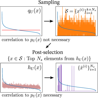
Let us denote as a probability distribution for sampling and as a distribution for post-selection. We now present the algorithm, illustrated in Fig. 1. Step 1. Choose an efficient classical sampler . Step 2. Generate samples from . Step 3. Compute for each sample. In this procedure, we require efficiently computable and correlated to . Step 4. Post-select and output samples whose ’s are largest out of samples 333Another possible way is to generate samples and post-select a single sample out of samples and iterate times, instead of generating and post-select samples at once. While we do not expect a significant difference, we employ the latter in this work consistently..
The principle behind the post-selection is that due to the correlation between and , we obtain samples likely to have a larger probability with respect to the ideal distribution by selecting the samples with larger . Thus, the most crucial step is to find correlated with the ideal distribution but easy to compute. Together with our numerical result below, the existence of such indicators might be related to hardness of heavy outcome generation in that the indicators enable us to generate heavy outcomes, where the heaviness means that its probability is larger than the median of probabilities 444We note that generating outcomes whose probabilities are larger than the median is sufficient to spoof the XEB because even running a quantum device can only generate heavy outcomes in this sense slightly better than the light outcomes [33].. Note that we do not compute the ideal probability in the entire procedure for sampling. We provide more discussions about the choice of and in Ref. [40].
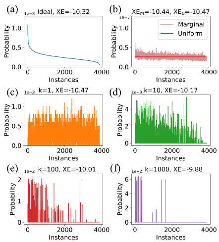
Spoofing XEB in GBS experiments.— To illustrate how the spoofing procedure operates in practice, we analyze the method for a small-size GBS circuit with the number of modes and the number of photons [12]. Here, we choose uniform distribution and first-order-marginal-based distribution , where is the ideal marginal probability of the th mode. Here, the marginal probabilities can be easily computed since the reduced state is a single-mode Gaussian state whose covariance matrix is a submatrix of the full covariance matrix [41]. Because the chosen perfectly recovers the first-order marginals of the ideal distribution by definition, it correlates with the ideal distribution. After computing all the ideal probabilities , we sort the outcomes in descending order. We also compute and and sort them in the same order as the ideal case. Although we use log XE for comparison with experiments in Refs. [11, 12], a similar result using linear XE is provided in Ref. [40].
As shown in Fig. 2(a) and (b), the ideal probability is likely to be large if is large, which clearly shows their correlation, while each XE of and is smaller than the ideal distribution. However, as the post-selection rate increases, the samples are concentrated on large probabilities of the ideal distribution, which clearly shows that our procedure selectively generates heavy outcomes. Especially for , the samples are highly concentrated on the heavy outcomes. Consequently, the spoofer’s XE is larger than the ideal probability. Therefore, one can attain a large XE by sampling heavy outcomes without directly simulating the desired circuit. Here, the XE might not monotonically increase as the post-selection rate because one might end up selecting less heavy outcomes. We also analyze the same procedure for Fock-state BS (FBS) using different in Ref [40].

Now, we consider intermediate-size circuits used for demonstrating quantum advantage in Ref. [12], where the experimental samples attain a larger XE than various mock-up distributions. Since XE is not an efficient verification method, the result based on the intermediate-scale circuits is claimed to be evidence of the quantum advantage of their largest circuit. Following Ref. [12], we normalize as , where and is the probability of obtaining photons from .
We emphasize that the XEB we employ is applied for each photon number sector instead of the entire sample set, consistently with the previous methods in experiments [10, 11, 12]. Therefore, it is not sensitive to the total photon number distribution. If we conduct the benchmarking for the entire set, a trivial way can spoof it by manipulating the total photon number distribution of a mock-up sampler so that the sampler generates samples from a particular sector having a larger probability of each outcome than other sectors on average. Meanwhile, we show in Ref. [40] that we can adjust our spoofer’s total number distribution to be consistent with the ideal case.
Figure 3 again shows that without post-selection, the XE is much smaller than the experimental samples’ XE from Ref. [12]. Meanwhile, for , the spoofer’s XE is much larger than the experiment for the wide range of photon numbers. Additionally, as the post-selection rate increases further, the difference becomes more significant. Based on the trend, we expect that such a gap may not close for the large photon number sectors. Similar results for different experiments [11] are provided in Ref. [40].
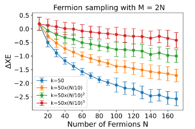
Prediction for larger systems.— Since XEB is computationally inefficient, it is demanding to check if the spoofer works even for larger systems. To predict its performance for large-size circuits and how the post-selection overhead scales, we consider a particular type of FS 555While the Fermionic sampling we consider is easy, there exists different types of Fermionic sampling which is proven to be hard under plausible assumptions [53], a variant of FBS (See Refs. [37, 40]). Since the FS is easy to simulate and its probabilities are easy to compute [37], it does not provide quantum advantage. Nevertheless, its similar structure to BS may enable us to predict a larger BS, since the key idea of our algorithm is to post-select heavy outcomes without computing the probability of the ideal distribution; thus it does not directly rely on the easiness of FS.
Figure 4 shows the result. We implement the same spoofer for FS with larger system sizes with post-selection rate differently to analyze the post-selection overhead and investigate the XE difference: . Although the XE from different choices of the post-selection rate varies, all the different cases’ XE difference gradually becomes negative as the system size grows. Such a trend may be caused because the first-order marginals’ correlation to the ideal distribution is not sufficiently large for larger system sizes. It implies that as the system size increases, the post-selection rate might have to increase, superpolynomially at worst. Even if this is true, since we are comparing the XE score against the ideal case and noise significantly decreases the XE of experiments (see below), it would be extremely difficult to surpass the score from our spoofer in the near future.
Evidence of efficiency of spoofing noisy BS.— We now provide evidence that our algorithm can efficiently spoof noisy BS experiments. To this end, we study the linear XE, , of ideal and noisy FBS, assuming a collision-free regime, i.e., . For the ideal case, i.e., [3], the average XE for Haar-random unitary is given by
| (2) |
Here, we approximated submatrices of large Haar-random unitary matrices by random Gaussian matrices, with following the complex normal distribution and used [3] and . Meanwhile, the XE of independent of is given by [40], where one can clearly see the additional factor for the ideal case.
We now analyze the behavior of the XE under partial distinguishability [43, 44, 40], one of the most important noise models in practice, describing partial overlaps of wave functions of different photons (See Refs. [43, 44, 40] for more details of the model.) The XE of BS under partial distinguishability with respect to the ideal distribution, normalized by the XE of an independent distribution, is bounded by [40]
| (3) |
Observe that even for constant , the normalized XE converges to , which only provides an additional constant factor , while the ideal score’s factor increases as . Clearly, the XE significantly decreases under experimental noise, suggesting that the experimental XE will be much smaller than the ideal case.
We now provide analytical evidence that the noisy XE might be attainable using our method. Since analyzing our algorithm’s output probability distribution is difficult due to post-selection, we consider a different probability distribution , which contains our algorithm’s core idea as it tends to generate heavy outcomes from . Effectively, a similar effect to post-selection is expected for , because the resulting probability favors large-probability outcomes from (we do not expect that we can sample from the distribution.). Thus, the power is associated with post-selection overhead . We show for linear XE that the distribution with a multinomial distribution , provides [40]
| (4) |
where the approximation holds for small and large . Since it suffices to achieve a constant factor due to noise from Eq. (3) and there are other types of noise such as loss [40], we expect that choosing a constant power , which may be interpreted as constant post-selection overhead , might be sufficient to spoof noisy BS unless the noise can be highly suppressed.
Comparison to existing spoofing methods.— Most existing methods for spoofing GBS work by attempting to model noisy experiments. It is often the case that noisy experiments converge to classically easy distribution [15, 18, 44, 24, 25, 23, 45]. These algorithms exploit this by sampling from this easy distribution. For example, G. Kalai claimed that noisy experimental boson sampler’s probabilities are approximable by low-degree polynomials [15]. Since then, there have been many subsequent proposals to take advantage of noise [44, 18]. Similarly, the algorithm in Ref. [25] aims to reproduce low-order marginals without recovering high-order marginals. Another method is to use the classical state because noise often transforms the output state to be close to classical states [46, 20, 23, 45].
Unlike the existing methods, our method’s goal is spoofing XEB instead of approximate simulation. Since XE increases by generating heavy outcomes, a large XE can be achieved without simulation. Thus, our approach does not necessarily work for other benchmarking that does not rely on heavy outcome generation, such as Bayesian test and correlation functions [47]. The Bayesian test employed in current GBS experiments as another evidence of quantum advantage [10, 11, 12] defines the score as
| (5) |
where is a sample set from experiment. A positive score implies that the experimental samples are more likely to be sampled from the ideal distribution than the mock-up distribution . Because the test requires the profile of the mock-up distribution and computing the post-selected distribution’s probability is difficult, it is not easy to perform Bayesian test against our method. Nevertheless, because our method favorably generates heavy outcomes, the output distribution may be highly concentrated. Thus, even if we can compute the probability distribution, our method is unlikely to pass the Bayesian test.
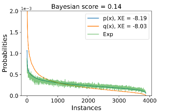
As an example that generates heavy outcomes but fails to pass Bayesian test, consider a mock-up distribution (without post-selection). Thus, generates heavier outcomes than with respect to , which guarantees to spoof the XE test, as shown in Fig. 5. However, since the mock-up distribution is farther than the ideal distribution to empirical experimental distribution, the Bayesian score becomes positive, implying that fails to pass the Bayesian test although it generates heavy outcomes.
Finally, our results spoofing the XE test do not imply that the experiments in Refs. [10, 11, 12] are easy to simulate because our algorithm’s goal is to spoof the test without simulation. Instead, the implication is that the XE scores may not be a proper measure as evidence of quantum advantage of BS. Our results open many questions about the verification of sampling tasks. First, making our method analytical is crucial to predict the asymptotic behavior of the method precisely. Second, it would also be interesting to apply the same method to other sampling tasks. Especially for RCS, finding a distribution that is correlated with the ideal distribution and easy to compute would be an important first step to applying the presented method. We emphasize again that although we chose relying on marginals, other various possible quantities may not necessarily rely on marginals. Also, since our algorithm is specialized to spoof the XE test, we do not expect it to pass other tests such as the Bayesian test. Hence, it would also be interesting to analyze the Bayesian test as well to see if it can be spoofed.
Acknowledgements.
We thank Benjamin Villalonga and Sergio Boixo for interesting and fruitful discussions. We acknowledge support from the ARO MURI (W911NF-16-1-0349, W911NF-21-1-0325), AFOSR MURI (FA9550-19-1-0399, FA9550-21-1-0209), DoE Q-NEXT, NSF (OMA-1936118, ERC-1941583, OMA-2137642), NTT Research, and the Packard Foundation (2020-71479). B.F. acknowledges support from AFOSR (FA9550-21-1-0008). This material is based upon work partially supported by the National Science Foundation under Grant CCF-2044923 (CAREER) and by the U.S. Department of Energy, Office of Science, National Quantum Information Science Research Centers (Q-NEXT). This material is also supported in part by the DOE QuantISED grant DE-SC0020360. The authors are also grateful for the support of the University of Chicago Research Computing Center for assistance with the numerical simulations carried out in this paper.References
- Shor [1994] P. W. Shor, Algorithms for quantum computation: discrete logarithms and factoring, in Proceedings 35th annual symposium on foundations of computer science (Ieee, 1994) pp. 124–134.
- Lloyd [1996] S. Lloyd, Universal quantum simulators, Science 273, 1073 (1996).
- Aaronson and Arkhipov [2011] S. Aaronson and A. Arkhipov, The computational complexity of linear optics, in Proceedings of the forty-third annual ACM symposium on Theory of computing (2011) pp. 333–342.
- Hamilton et al. [2017] C. S. Hamilton, R. Kruse, L. Sansoni, S. Barkhofen, C. Silberhorn, and I. Jex, Gaussian boson sampling, Physical review letters 119, 170501 (2017).
- Bouland et al. [2019] A. Bouland, B. Fefferman, C. Nirkhe, and U. Vazirani, On the complexity and verification of quantum random circuit sampling, Nature Physics 15, 159 (2019).
- Deshpande et al. [2022] A. Deshpande, A. Mehta, T. Vincent, N. Quesada, M. Hinsche, M. Ioannou, L. Madsen, J. Lavoie, H. Qi, J. Eisert, et al., Quantum computational advantage via high-dimensional gaussian boson sampling, Science advances 8, eabi7894 (2022).
- Arute et al. [2019] F. Arute, K. Arya, R. Babbush, D. Bacon, J. C. Bardin, R. Barends, R. Biswas, S. Boixo, F. G. Brandao, D. A. Buell, et al., Quantum supremacy using a programmable superconducting processor, Nature 574, 505 (2019).
- Wu et al. [2021] Y. Wu, W.-S. Bao, S. Cao, F. Chen, M.-C. Chen, X. Chen, T.-H. Chung, H. Deng, Y. Du, D. Fan, et al., Strong quantum computational advantage using a superconducting quantum processor, Physical review letters 127, 180501 (2021).
- Morvan et al. [2023] A. Morvan, B. Villalonga, X. Mi, S. Mandrà, A. Bengtsson, P. Klimov, Z. Chen, S. Hong, C. Erickson, I. Drozdov, et al., Phase transition in random circuit sampling, arXiv preprint arXiv:2304.11119 (2023).
- Zhong et al. [2020] H.-S. Zhong, H. Wang, Y.-H. Deng, M.-C. Chen, L.-C. Peng, Y.-H. Luo, J. Qin, D. Wu, X. Ding, Y. Hu, et al., Quantum computational advantage using photons, Science 370, 1460 (2020).
- Zhong et al. [2021] H.-S. Zhong, Y.-H. Deng, J. Qin, H. Wang, M.-C. Chen, L.-C. Peng, Y.-H. Luo, D. Wu, S.-Q. Gong, H. Su, et al., Phase-programmable gaussian boson sampling using stimulated squeezed light, Physical review letters 127, 180502 (2021).
- Madsen et al. [2022] L. S. Madsen, F. Laudenbach, M. F. Askarani, F. Rortais, T. Vincent, J. F. Bulmer, F. M. Miatto, L. Neuhaus, L. G. Helt, M. J. Collins, et al., Quantum computational advantage with a programmable photonic processor, Nature 606, 75 (2022).
- Deng et al. [2023] Y.-H. Deng, Y.-C. Gu, H.-L. Liu, S.-Q. Gong, H. Su, Z.-J. Zhang, H.-Y. Tang, M.-H. Jia, J.-M. Xu, M.-C. Chen, et al., Gaussian boson sampling with pseudo-photon-number resolving detectors and quantum computational advantage, arXiv preprint arXiv:2304.12240 (2023).
- Aharonov et al. [1996] D. Aharonov, M. Ben-Or, R. Impagliazzo, and N. Nisan, Limitations of noisy reversible computation, arXiv preprint quant-ph/9611028 (1996).
- Kalai and Kindler [2014] G. Kalai and G. Kindler, Gaussian noise sensitivity and bosonsampling, arXiv preprint arXiv:1409.3093 (2014).
- Bremner et al. [2017] M. J. Bremner, A. Montanaro, and D. J. Shepherd, Achieving quantum supremacy with sparse and noisy commuting quantum computations, Quantum 1, 8 (2017).
- Gao and Duan [2018] X. Gao and L. Duan, Efficient classical simulation of noisy quantum computation, arXiv preprint arXiv:1810.03176 (2018).
- Renema et al. [2018a] J. Renema, V. Shchesnovich, and R. Garcia-Patron, Classical simulability of noisy boson sampling, arXiv preprint arXiv:1809.01953 (2018a).
- Shchesnovich [2019] V. S. Shchesnovich, Noise in boson sampling and the threshold of efficient classical simulatability, Physical Review A 100, 012340 (2019).
- García-Patrón et al. [2019] R. García-Patrón, J. J. Renema, and V. Shchesnovich, Simulating boson sampling in lossy architectures, Quantum 3, 169 (2019).
- Noh et al. [2020] K. Noh, L. Jiang, and B. Fefferman, Efficient classical simulation of noisy random quantum circuits in one dimension, Quantum 4, 318 (2020).
- Takahashi et al. [2021] Y. Takahashi, Y. Takeuchi, and S. Tani, Classically simulating quantum circuits with local depolarizing noise, Theoretical Computer Science 893, 117 (2021).
- Qi et al. [2020] H. Qi, D. J. Brod, N. Quesada, and R. García-Patrón, Regimes of classical simulability for noisy gaussian boson sampling, Physical review letters 124, 100502 (2020).
- Oh et al. [2021] C. Oh, K. Noh, B. Fefferman, and L. Jiang, Classical simulation of lossy boson sampling using matrix product operators, Physical Review A 104, 022407 (2021).
- Villalonga et al. [2021] B. Villalonga, M. Y. Niu, L. Li, H. Neven, J. C. Platt, V. N. Smelyanskiy, and S. Boixo, Efficient approximation of experimental gaussian boson sampling, arXiv preprint arXiv:2109.11525 (2021).
- Aharonov et al. [2022] D. Aharonov, X. Gao, Z. Landau, Y. Liu, and U. Vazirani, A polynomial-time classical algorithm for noisy random circuit sampling, arXiv preprint arXiv:2211.03999 (2022).
- Oh et al. [2023a] C. Oh, L. Jiang, and B. Fefferman, On classical simulation algorithms for noisy boson sampling, arXiv preprint arXiv:2301.11532 (2023a).
- Liu et al. [2023] M. Liu, C. Oh, J. Liu, L. Jiang, and Y. Alexeev, Complexity of gaussian boson sampling with tensor networks, arXiv preprint arXiv:2301.12814 (2023).
- Oh et al. [2023b] C. Oh, M. Liu, Y. Alexxev, B. Fefferman, and L. Jiang, Tensor network algorithm for simulating experimental gaussian boson sampling, arXiv preprint arXiv:2306.03709 (2023b).
- Boixo et al. [2018] S. Boixo, S. V. Isakov, V. N. Smelyanskiy, R. Babbush, N. Ding, Z. Jiang, M. J. Bremner, J. M. Martinis, and H. Neven, Characterizing quantum supremacy in near-term devices, Nature Physics 14, 595 (2018).
- Note [1] XEB is sample-efficient in the sense that it does not require an exponentially large number of samples while it is computationally inefficient because computing the ideal output probability requires exponential time.
- Aaronson and Chen [2016] S. Aaronson and L. Chen, Complexity-theoretic foundations of quantum supremacy experiments, arXiv preprint arXiv:1612.05903 (2016).
- Aaronson and Gunn [2019] S. Aaronson and S. Gunn, On the classical hardness of spoofing linear cross-entropy benchmarking, arXiv preprint arXiv:1910.12085 (2019).
- Gao et al. [2021] X. Gao, M. Kalinowski, C.-N. Chou, M. D. Lukin, B. Barak, and S. Choi, Limitations of linear cross-entropy as a measure for quantum advantage, arXiv preprint arXiv:2112.01657 (2021).
- Pan et al. [2021] F. Pan, K. Chen, and P. Zhang, Solving the sampling problem of the sycamore quantum supremacy circuits, arXiv preprint arXiv:2111.03011 (2021).
- Note [2] Other benchmarking methods employed [10, 11, 12, 13], such as Bayesian test and correlator methods, also do not have rigorous evidence for hardness. Also, the Bayesian test is genuinely implemented against adversarial samplers; thus, it cannot rule out all possible classical algorithms. We emphasize that the current GBS experiments employ XEB against certain adversarial samplers because we do not know the ideal score.
- Aaronson and Arkhipov [2013] S. Aaronson and A. Arkhipov, Bosonsampling is far from uniform, arXiv preprint arXiv:1309.7460 (2013).
- Note [3] Another possible way is to generate samples and post-select a single sample out of samples and iterate times, instead of generating and post-select samples at once. While we do not expect a significant difference, we employ the latter in this work consistently.
- Note [4] We note that generating outcomes whose probabilities are larger than the median is sufficient to spoof the XEB because even running a quantum device can only generate heavy outcomes in this sense slightly better than the light outcomes [33].
- [40] See supplemental material for more discussion about the spoofing algorithm and more numerical results for different experiments and linear cross entropy measure, which includes Refs. [48, 49, 50, 51, 52].
- Serafini [2017] A. Serafini, Quantum continuous variables: a primer of theoretical methods (CRC press, 2017).
- Note [5] While the Fermionic sampling we consider is easy, there exists different types of Fermionic sampling which is proven to be hard under plausible assumptions [53].
- Tichy [2015] M. C. Tichy, Sampling of partially distinguishable bosons and the relation to the multidimensional permanent, Physical Review A 91, 022316 (2015).
- Renema et al. [2018b] J. J. Renema, A. Menssen, W. R. Clements, G. Triginer, W. S. Kolthammer, and I. A. Walmsley, Efficient classical algorithm for boson sampling with partially distinguishable photons, Physical review letters 120, 220502 (2018b).
- Martńez-Cifuentes et al. [2022] J. Martńez-Cifuentes, K. Fonseca-Romero, and N. Quesada, Classical models are a better explanation of the jiuzhang gaussian boson samplers than their targeted squeezed light models, arXiv preprint arXiv:2207.10058 (2022).
- Oszmaniec and Brod [2018] M. Oszmaniec and D. J. Brod, Classical simulation of photonic linear optics with lost particles, New Journal of Physics 20, 092002 (2018).
- Phillips et al. [2019] D. Phillips, M. Walschaers, J. Renema, I. Walmsley, N. Treps, and J. Sperling, Benchmarking of gaussian boson sampling using two-point correlators, Physical Review A 99, 023836 (2019).
- Oh et al. [2022] C. Oh, Y. Lim, B. Fefferman, and L. Jiang, Classical simulation of boson sampling based on graph structure, Physical Review Letters 128, 190501 (2022).
- Popova and Rubtsov [2022] A. Popova and A. Rubtsov, Cracking the quantum advantage threshold for gaussian boson sampling, in Quantum 2.0 (Optica Publishing Group, 2022) pp. QW2A–15.
- Drummond et al. [2022] P. D. Drummond, B. Opanchuk, A. Dellios, and M. D. Reid, Simulating complex networks in phase space: Gaussian boson sampling, Physical Review A 105, 012427 (2022).
- Ivanov and Gurvits [2020] D. A. Ivanov and L. Gurvits, Complexity of full counting statistics of free quantum particles in product states, Physical Review A 101, 012303 (2020).
- Tichy et al. [2014] M. C. Tichy, K. Mayer, A. Buchleitner, and K. Mølmer, Stringent and efficient assessment of boson-sampling devices, Physical review letters 113, 020502 (2014).
- Oszmaniec et al. [2022] M. Oszmaniec, N. Dangniam, M. E. Morales, and Z. Zimborás, Fermion sampling: a robust quantum computational advantage scheme using fermionic linear optics and magic input states, PRX Quantum 3, 020328 (2022).