Beyond Ultra-diffuse Galaxies. I. Mass–Size Outliers among the Satellites of Milky Way Analogs

Abstract

Large diffuse galaxies are hard to find, but understanding the environments where they live, their numbers, and ultimately their origins, is of intense interest and importance for galaxy formation and evolution. Using Subaru’s Hyper Suprime-Cam Strategic Survey Program, we perform a systematic search for low surface brightness galaxies and present novel and effective methods for detecting and modeling them. As a case study, we surveyed 922 Milky Way analogs in the nearby Universe ($0.01<z<0.04$) and built a large sample of satellite galaxies that are outliers in the mass–size relation. These “ultra-puffy” galaxies (UPGs), defined to be $1.5\sigma$ above the average mass–size relation, represent the tail of the satellite size distribution. We find that each MW analog hosts $N_{\rm UPG}=0.31\pm 0.05$ ultra-puffy galaxies on average, which is consistent with but slightly lower than the observed abundance at this halo mass in the Local Volume. We also construct a sample of ultra-diffuse galaxies (UDGs) in MW analogs and find an abundance of $N_{\rm UDG}=0.44\pm 0.05$ per host. With literature results, we confirm that the UDG abundance scales with the host halo mass following a sublinear power law. We argue that our definition for ultra-puffy galaxies, which is based on the mass–size relation, is more physically motivated than the common definition of ultra-diffuse galaxies, which depends on the surface brightness and size cuts and thus yields different surface mass density cuts for quenched and star-forming galaxies.

1 Introduction

In a variety of galaxies in the Universe, there is an interesting subset of galaxies with low surface brightness (dubbed low surface brightness galaxies or LSBGs, e.g., Sandage & Binggeli, 1984; Caldwell & Bothun, 1987; Impey et al., 1988; McGaugh et al., 1995; Dalcanton et al., 1997a). Recently, new excitement has been generated by the discovery of a large population of ultra-diffuse galaxies (UDGs) in the Coma cluster (van Dokkum et al., 2015), accompanied by many other works on detecting UDGs in clusters (e.g., Koda et al., 2015; Mihos et al., 2015; Yagi et al., 2016; van der Burg et al., 2016, 2017; Lee et al., 2017; Mancera Piña et al., 2018; Zaritsky et al., 2019; Danieli & van Dokkum, 2019), groups (e.g., Román & Trujillo, 2017a; Mao et al., 2021; Román et al., 2021; Carlsten et al., 2022a), and the field (e.g., Leisman et al., 2017; Greco et al., 2018; Román et al., 2019; Prole et al., 2019; Tanoglidis et al., 2021; Kadowaki et al., 2021). There have been a variety of studies of these diffuse galaxy systems, ranging from their dark matter content (e.g., Mowla et al., 2017; van Dokkum et al., 2018, 2019; Danieli et al., 2019; Wasserman et al., 2019; Mancera Piña et al., 2019b; Keim et al., 2022; Mancera Piña et al., 2022b; Kong et al., 2022), to globular cluster populations (e.g., van Dokkum et al., 2017; Somalwar et al., 2020; Forbes et al., 2020; Danieli et al., 2022; Gannon et al., 2022; van Dokkum et al., 2022a; Gannon et al., 2022), and stellar populations (e.g., Gu et al., 2018; Ferré-Mateu et al., 2018; Pandya et al., 2018; Villaume et al., 2022). We refer to LSBGs as objects selected purely based on surface brightness without distance information. With known distances, people define UDGs to be galaxies with large sizes ($r_{e}>1.5$ kpc) and low surface brightnesses ($\mu_{0}(g)>24.0\ \mathrm{mag\ arcsec}^{-2}$), and thus UDGs are outliers in size and surface brightness compared to normal dwarf galaxies. A central question about LSBGs, including UDGs, is what causes them to be outliers from the average mass–size relation of dwarf galaxies.

Various mechanisms have been proposed to explain the presence of large, diffuse galaxies (as mass–size outliers) across different environments. In the field (i.e, in isolation), their large sizes might be a result of stellar feedback (Di Cintio et al., 2017; Chan et al., 2018), early galaxy mergers (Wright et al., 2021), passing into and out of a more massive halo (so-called backsplash satellites; Benavides et al. 2021), or of inhabiting halos with higher spins (Dalcanton et al., 1997b; Amorisco & Loeb, 2016; Liao et al., 2019; Mancera Piña et al., 2020; Benavides et al., 2022; Kong et al., 2022). In groups and clusters, their large sizes may ensue from tidal heating near pericenter (Jiang et al., 2019), via adiabatic expansion due to mass loss (Tremmel et al., 2020), or even via a bullet-dwarf collision (van Dokkum et al., 2022b, a). Despite theoretical advances, it is still an open question how mass–size outliers like UDGs are formed. It is also unclear whether mass–size outliers belong to a distinct class of galaxies or are just a natural extension of dwarf systems to lower surface brightness or larger sizes (e.g., Greene et al., 2022). A straightforward way to answer these questions is to compare mass–size outliers with “normal” low-mass galaxies, which have been studied extensively.

Our best understanding of the low mass galaxy regime comes from the satellite system of our Milky Way (MW) and the Local Group (LG; e.g., McConnachie, 2012; Simon, 2019). With the advent of deep sky surveys and dedicated spectroscopic programs, we are now in a position to also map the satellite systems of MW analogs (typically defined as galaxies having similar stellar mass or halo mass to MW) in the Local Volume and nearby Universe. The Satellites Around Galactic Analogs survey (SAGA; Geha et al. 2017; Mao et al. 2021) is designed to spectroscopically confirm the satellites of 100 MW analogs at 20–40 Mpc. The Exploration of Local VolumE Satellites survey (ELVES; Carlsten et al. 2021, 2022b, 2022a) uses deep imaging data to identify satellite candidates of MW-like hosts in the Local Volume (LV; $D<12$ Mpc) and estimate surface brightness fluctuation distances from images to confirm their association with their hosts. Having these satellites of MW analogs as a reference frame, we can contrast them with the mass–size outliers in the same environment to understand the formation of large diffuse galaxies. However, there are only $\sim 40$ confirmed UDGs associated with MW analogs in the literature (Román & Trujillo, 2017a; Cohen et al., 2018; Mao et al., 2021; Carlsten et al., 2022a; Nashimoto et al., 2022; Karunakaran & Zaritsky, 2022). Therefore, a larger sample of mass–size outliers associated with MW-like hosts is needed to conduct such a comparison between the mass–size outliers and the normal satellites.

The goal of this paper is to find and study large diffuse satellite galaxies in the context of MW analogs. Leveraging the depth and wide sky coverage of Hyper Suprime-Cam (HSC) Subaru Strategic Program (Aihara et al., 2018) imaging data, we perform a search for LSBGs using novel methods in detection, false-positive identification, and modeling. We further build a large sample of mass–size outliers that are likely satellites of MW-mass hosts in the nearby Universe. We propose a new definition of mass–size outliers, dubbed “ultra-puffy galaxies” (UPGs), based on the observed mass–size relation of satellites of MW analogs in the LV using the ELVES sample. This concept is less affected by the galaxy color and provides a robust avenue to study the mass–size outlier population. We calculate the abundances of mass–size outliers in MW analogs and compare them with their abundances in other environments. Our results seek to shed light on the role of the environment on the formation of large diffuse dwarf galaxies.

The layout of this paper is as follows. Section 2 describes the data used in this work. In Section 3, we describe the LSBG search in HSC data, including source detection (§3.1), deblending (§3.2), modeling (§3.3), completeness, and uncertainty (§3.4). In Section 4, we propose a new definition of large and diffuse galaxies (UPGs) and present our UDG and UPG samples. In Section 5, we compare the UDGs and UPGs on the mass–size plane. We calculate their abundances and compare them with the literature (§5.2). Based on these results, we further argue that we should move beyond UDGs and adopt the UPG definition in Section 6. Section 7 presents a summary of this work and prospects for the future. In a companion paper (Li et al., 2023), we discuss the size distributions, spatial distributions, and quenching of UDGs and UPGs.

In this work, we refer to mass–size outliers (including both UDGs and UPGs) as galaxies with large physical sizes compared to normal dwarf galaxies. We adopt a flat $\Lambda$CDM cosmology from Planck Collaboration et al. (2016) with $\Omega_{\rm m}=0.307$ and $H_{0}=67.7\$km s^-1 Mpc^-1. We use the AB system (Oke & Gunn, 1983) for magnitudes. The stellar mass used in this work is based on a Chabrier (2003) initial mass function.

2 Data

2.1 The Hyper Suprime-Cam Subaru Strategic Program

The Hyper Suprime-Cam Subaru Strategic Program (HSC-SSP, hereafter the HSC survey; Aihara et al. 2018) is an optical imaging survey using the 8.2 m Subaru telescope and the Hyper Suprime-Camera (Miyazaki et al., 2012, 2018). The Wide layer is designed to cover $\sim 1000\ \rm{deg}^{2}$ of the sky in five broad bands ($grizy$), reaching a depth of $g=26.6$ mag, $r=26.2$ mag and $i=26.2$ mag ($5\sigma$ point-source detection). HSC data are processed using hscPipe (Bosch et al., 2018), which is a customized version of the Vera Rubin Observatory Legacy Survey of Space and Time (LSST) pipeline (Jurić et al., 2017).

In this work, we use the Wide layer of the co-added data from the Public Data Release 2 (PDR2, also known as S18A, Aihara et al. 2018) of the HSC survey. It covers $\sim 300\ \rm{deg}^{2}$ in all five bands, which is 1.5 times larger than the dataset (S16A) analyzed in Greco et al. (2018). One of the key improvements made in PDR2 is the sky background subtraction. Compared with previous data releases, PDR2 adopted a full focal plane sky subtraction algorithm to overcome the oversubtraction of the local sky background around bright objects (Aihara et al., 2018; Li et al., 2022). The unprecedented depth and careful sky subtraction make PDR2 an ideal dataset to study low surface brightness galaxies. In this work we take the point-spread function (PSF) models in hscPipe (Bosch et al., 2018), where the Point Spread Function Extractor (PSFEx; Bertin, 2011) takes a star catalog and generates the PSF model.

2.2 NASA-Sloan Atlas

We use the NASA-Sloan Atlas (NSA, Blanton et al. 2005, 2011) to select galaxies that are analogous to our Milky Way based on their stellar mass (see §4.1); then we match the LSBGs to these MW analogs. The NSA catalog provides various physical properties of galaxies in the nearby Universe as derived from the Sloan Digital Sky Survey (SDSS; York et al., 2000). We use the most recent version of the NSA catalog (v1_0_1) which contains about $640,000$ galaxies out to $z<0.15$. This version also updates the aperture photometry to elliptical Petrosian photometry, which is considered to be more reliable than the photometry used in the older versions. In this paper, we use the stellar masses derived from the elliptical Petrosian photometry using kcorrect v4_2 (Blanton & Roweis, 2007). The redshifts of the galaxies in the NSA come from several spectroscopic surveys, H I gas surveys, or direct distance measurements.

3 LSBG Search in HSC PDR2

Continuing the work of Greco et al. (2018, hereafter G18), we conducted a systematic search for low surface brightness galaxies in the HSC PDR2 data, which covers $\sim 1.5$ times the sky area of G18. The schematic of the searching method in this paper remains similar to that in G18, but we do improve the search completeness and purity by adding several new steps, which are highlighted in this section. We outline the major steps below and refer the readers who are already familiar with the algorithms in LSBG searches to §4 for the mass–size outlier sample construction.

1. Source detection (§3.1): We run SourceExtractor (Bertin & Arnouts, 1996) on the co-added images after removing bright extended sources. Then we apply an initial size and color cut based on the output catalog.

2. Deblending (§3.2): We remove false positives that are not likely to be LSBGs by running scarlet (Melchior et al., 2018). We use the scarlet models to define color–size–morphology–surface brightness cuts. This step removes roughly 98% of false positives.

3. Modeling (§3.3): We fit a parametric model to the LSBGs to estimate their properties, including their sizes, total magnitudes, and average surface brightnesses.

4. Completeness and measurement biases and uncertainties (§3.4) are characterized by injecting mock Sérsic galaxies into images and recovering them following the procedures described above.

The number of objects remaining after each step is shown in Table 1. Our source detection pipeline hugs and the deblending and modeling code kuaizi are open-source and available online.

Table 1: LSBG Search Steps and Number of Remaining Objects After Each Step

Process	Description	Remaining Objects
Initial detection	§3.1	86,002
Matching with MW analogs at $0.01<z<0.04$	§4.1	10,579
Deblending	§3.2	2673
Spergel profile modeling	§3.3, §4.1	2510
Completeness	§3.4,§D	2510
Measurement error and uncertainty	§3.4,§D	2510
Mass–size outlier selection	§4.2	337 UPGs, 412 UDGs

3.1 Source Detection

G18 performed a search for LSBGs in the first $\sim 200$ deg² of the HSC survey and uncovered 781 LSBGs. We continued the work in G18 and extended the search to the HSC PDR2 data, which cover $\sim 300\ \rm{deg}^{2}$ and have sky subtraction better suited for LSB studies compared to prior data releases. We follow the same method for source detection as in G18 but make several updates to accommodate the PDR2 data. These updates are guided by both our understanding of PDR2 data and completeness tests using mock galaxies. We summarize the main steps of the LSBG search method here and refer the interested reader to G18 and Appendix A for more details.

We start by replacing the bright sources and their associated LSB outskirts with sky noise. Bright objects and their diffuse light are identified using surface brightness thresholding. We run an additional detection using sep (Barbary, 2016) to remove small compact sources and noisy peaks and replace their footprints with sky noise. Then we use SourceExtractor to detect sources on the “cleaned” images with a low detection threshold. Taking the output catalog from SourceExtractor, we apply an initial selection based on the size, color, and peakiness of objects.

After these steps, we have an initial sample that contains 86,002 LSBG candidates. We obtain 4 times more sources per square degree ($\sim 280\ \mathrm{deg}^{-2}$) than G18 mainly because HSC PDR2 has sky subtraction suited for finding LSB features. Our detection here is more inclusive of larger objects, and our size cut is less restrictive for small objects. Among these objects, there are still many false positives, including shredded galaxy outskirts, tidal features, Galactic cirrus, and blended compact sources. Therefore, we perform an extra “deblending” step to further remove false positives.

3.2 Deblending

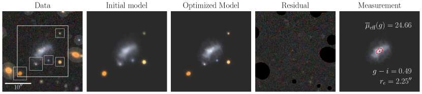
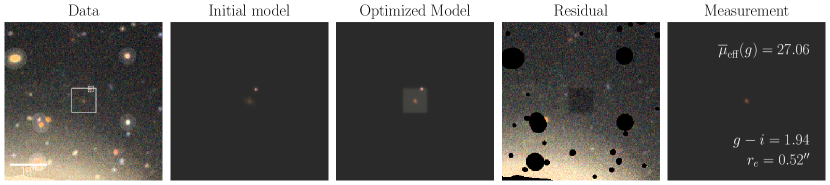
Figure 1: Demonstration of the deblending step described in §3.2 and §B. Here we show two objects from our initial sample: the one shown in the top panels is a blue LSBG, whereas the one shown in the bottom is a false positive, which is a blend between a high-$z$ galaxy and galaxy outskirts. The first columns show the $griz$ color-composite images with the bounding boxes overlaid. The objects covered by the gray shades are masked during fitting. The remaining columns show the initial model, the optimized model (PSF convolved), the residual image, and the optimized model of the target galaxy only. The red dashed circle in the rightmost column denotes the measured half-light radius.

Removing false positives from the initial sample while retaining high completeness is one of the major challenges in LSBG searches (e.g., van Dokkum et al., 2015; Koda et al., 2015; Yagi et al., 2016; Greco et al., 2018; Geha et al., 2017; Zaritsky et al., 2019, 2021; Tanoglidis et al., 2021; Zaritsky et al., 2022). A common type of false positives occurs when point-like sources are blended with diffuse light from background galaxies or the LSB outskirts of stars and galaxies. Our initial detection cannot distinguish them from real LSBGs. In order to identify and remove these objects from our sample, we perform nonparametric modeling of all LSBG candidates using scarlet (Melchior et al., 2018) and design an effective metric to remove false positives.

3.2.1 Scarlet fitting

Scarlet is a deblending and modeling tool designed for multiband and multiresolution imaging data. It utilizes color and morphology information to separate blended objects and model objects in a nonparametric fashion. In the following, we briefly summarize how scarlet works, and we refer the interested readers to Melchior et al. (2018, 2021) and the online documentation for more details.

In scarlet, each source $k$ in the cutout is described by a morphology image $S_{k}$ and a spectral energy distribution (SED) vector $A_{k}$. The multi-band images are represented as $Y$. The goal of the modeling is to minimize the objective function $f=\frac{1}{2}||Y-P\ast(\sum_{k}A_{k}^{\top}\times S_{k})||^{2}$ under certain constraints, where $P$ is the PSF and $*$ is convolution. The morphology image of each source is limited by a bounding box. We assume two constraints when running scarlet: all sources have positive fluxes (positivity constraint), and the light profiles of all sources monotonically decrease from the center to the outskirts (monotonicity constraint). The monotonicity constraint is oversimplified for well-resolved galaxies with complicated structures, but for objects in our sample, this assumption still holds for most cases and provides an effective and robust way to deblend overlapping sources. We refer to this modeling method as vanilla scarlet.

We use vanilla scarlet to model the LSBG candidate, and the structural and morphological parameters are then used to exclude false positives from our LSBG sample. In the following, we briefly describe how we detect peaks on the image to initialize and optimize scarlet models. We refer the readers to Appendix B for a more detailed description.

The deblending step is designed to model the sources in the vicinity of the LSBG candidate. Therefore, we run sep on the $griz$-combined image to detect objects (i.e., peaks) around the LSBG candidate. Objects that are close to the LSBG candidate are modeled using scarlet models. The models are initialized based on the smoothed image to capture the LSB outskirts of the target galaxy. Then the models are optimized using the adaptive proximal gradient method (Melchior et al., 2019). Typically, convergence is achieved after $\sim 50$ steps of optimization, and the whole modeling process takes about 40s for a typical LSBG.

The deblending procedures are demonstrated in Figure 1 with two distinct examples. The one shown in the top panels is a blue LSBG, whereas the one shown on the bottom is a high-$z$ galaxy blended with the outskirts of a nearby galaxy, which falls in our initial sample as a false positive.

We note that the optimized model of the blue LSBG captures its color and morphology quite well. For the false-positive case, the optimized model has a notable bright background because we model the sky together with all other sources. The model for the target itself is actually very red and compact. It passes our initial selection because the galaxy outskirts are shredded by SourceExtractor and happen to have a large size and similar color to our LSB galaxies. However, once modeled using scarlet, it becomes clear that this is just a false-positive detection and should be removed. A rubric based on the scarlet model is therefore needed to help us identify and exclude the false positives.

3.2.2 False-positive Removal

After running vanilla scarlet for LSBG candidates, the target object is successfully deblended from nearby sources. Unlike other parametric modeling methods, the nonparametric scarlet model is flexible enough to adequately represent galaxies with complex structures. However, the nonparametric nature of the code means that we have to make additional measurements to quantify the size and shape of the scarlet model. As shown in the rightmost column of Figure 1, we isolate the model of the target object and analyze it using statmorph (Rodriguez-Gomez et al., 2019). The purpose of this analysis is to extract the structural and morphological parameters of the target object. We further use these diagnostics to remove false positives.

Statmorph calculates non-parametric morphological and structural parameters, including effective radius, concentration-asymmetry-smoothness statistics (CAS; Conselice, 2003), and Gini-M20 (Abraham et al., 2003; Lotz et al., 2004). The measurement requires an image, a variance map, and a PSF. For our purpose, the “image” is just the scarlet model convolved with the observed PSF. The variance map and PSF are taken from HSC cutouts. We also force the sky level in Statmorph to be zero because the sky has already been fit when running vanilla scarlet.

One of the most important diagnostics is the effective radius of the object. In this paper, we refer to the effective radius as the circularized effective radius $r_{e}$, defined as the $r_{e}=r_{\rm eff,sma}\sqrt{b/a}$ where $r_{\rm eff,sma}$ is the effective radius measured along the semi-major axis of the aligned elliptical isophotes, and $b/a$ is the axis ratio of the isophotes. In statmorph, the effective radius is calculated using elliptical apertures, where the ellipticity $\varepsilon$ is determined by calculating the second moment of the image. The total magnitudes are simply calculated by summing up the model flux in each band, and colors are defined using total magnitudes. A Galactic extinction correction is not applied at this point. The central surface brightness $\mu_{0}$ is measured by linearly extrapolating the surface brightness profile to $r\to 0$ using the scipy interpolation function (Jones et al., 2001). We define the average surface brightness within the effective radius as

$$\overline{\mu}_{\rm eff}=m+2.5\log_{10}(2\pi r_{e}^{2}),$$ (1)

where $m$ is the total magnitude.

We also use the Gini-M20 and CAS statistics. The Gini coefficient and M20 statistics (Abraham et al., 2003; Lotz et al., 2004) quantify how concentrated/extended the flux distribution is across the image. The CAS statistics characterize the concentration $C$, asymmetry $A$, and smoothness $S$ of the light distribution of the object. We refer the reader to Rodriguez-Gomez et al. (2019) for more details on their definitions and implementations.

To better guide us on how to use these diagnostics, we visually inspect a subset of LSBG candidates in our initial sample (§3.1) and use the classification results to help construct the metrics. More specifically, we randomly select 5000 LSBG candidates that are matched with a MW-like host at $0.01<z<0.04$ from the NSA catalog (see §4.1 for details). We run vanilla scarlet for all of them and measure the structural and morphological parameters as described above. Then we do visual inspections of the $griz$ color-composite images with 0$\farcm$5 on a side. False positives, including tidal streams, galaxy outskirts, blends, and other artifacts (dubbed junk), are identified during the visual inspection by coauthors J.E.G., J.G., S.H., R.B., K.C., A.G., and E.K-F. Each object has been inspected by at least two people. In the end, an object is classified as junk if the number of votes as junk is larger than the number of votes as nonjunk. In total, there are 1661 objects classified as junk. The visual inspection is summarized in Table 2.

We first apply the following selection cuts to remove false positives and background galaxies. They are motivated based on the knowledge of the color distribution of LSBGs (e.g., Geha et al., 2017; Greco et al., 2018; Zaritsky et al., 2019; Tanoglidis et al., 2021) and survey completeness in size and surface brightness (§3.4).

• Color:

  $$0.0<g-i<1.2,\quad|(g-r)-0.7\cdot(g-i)|<0.25$$

• Size:

  $$1.8\arcsec<r_{e}<12\arcsec$$

• Surface brightness:

  $$\mu_{0}(g)>22.5,\quad 23.0<\overline{\mu}_{\mathrm{eff}}(g)<27.5\ \mathrm{mag\ arcsec}^{-2}.$$

The color cuts here are more restrictive than the one used in the initial detection (Sec 3.1) to further remove junk and high redshift galaxies. We not only remove objects with small sizes but also exclude objects with large sizes and very low surface brightness because they are mostly spurious objects. After such cuts, there are 200 junk and 1407 non-junk remaining. The color-size-surface brightness cuts remove 88% of junk and 58% of nonjunk. We note that although we lose a lot of nonjunk objects, most of them are small, red objects, which are not likely to be LSBGs of our interest.

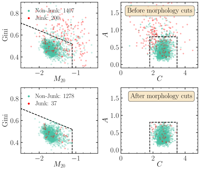
Figure 2: Distribution of scarlet morphological measurements for the LSBG candidates from our initial sample. The sample after the color–size–surface brightness cuts is shown in the top panels. We further remove false positives (junk; highlighted in red) by selecting their morphological parameters (dashed boxes). Morphology cuts (bottom panels) remove another 82% of junk. In total, 98% of false positives are removed in the deblending step.

We further use these visual inspection results to inform how to use morphological diagnostics. In the top panels of Figure 2, we show the distributions of junk (red) and nonjunk (green) in the parameter space spanned by four morphological parameters. There is still a significant amount of junk with high $M_{20}$, Gini coefficient, and asymmetry. Therefore, we add another set of selection cuts to further remove junk:

• Morphology:

  $$\varepsilon<0.65,\quad\mathrm{Gini}<0.70,\quad M_{20}<-1.1,$$

  $$\mathrm{Gini}<-0.136\cdot M_{20}+0.37,$$

  $$1.8<C<3.5,\quad A<0.8.$$

The slanted demarcation line on the Gini-$M_{20}$ diagram is motivated by the line used in Lotz et al. (2008) to separate merging galaxies from normal galaxies. The bottom panels in Figure 2 show the objects after applying the morphology selections, which remove another 82% of junk while only removing 9% of nonjunk. Such morphology cuts (shown as dashed lines in Figure 2) effectively help us remove false positives that are not likely to be LSBGs of interest.

In this way, we obtain an LSBG sample with high purity, where 98% of the false positives are removed (see Table 2). Therefore, our empirical selection based on the nonparametric measurements on the scarlet models successfully removes most of the false positives and a large fraction of small red galaxies (most likely background galaxies) in our initial sample. Furthermore, the completeness of the real LSBG detection remains high. In §3.4, we characterize the completeness of this “deblending” step by injecting mock Sérsic galaxies, and we achieve $\sim 80\%$ completeness at $\overline{\mu}_{\mathrm{eff}}(g)=27.0\ \mathrm{mag\ arcsec}^{-2}$ and $>50\%$ completeness at $\overline{\mu}_{\mathrm{eff}}(g)=27.5\ \mathrm{mag\ arcsec}^{-2}$ (Fig. 3). We emphasize that the vanilla scarlet modeling and nonparametric measurements are not designed to measure the structural properties of the galaxies. They are used only as a diagnostic tool to remove false positives. We perform more detailed modeling in §3.3 to measure galaxy properties for science.

Table 2: Number of Objects Remaining after Each Deblending Cut

Process	# junk	# nonjunk	# Total
Visual inspection	1661	3339	5000
Color–size–surface brightness cuts	200	1407	1607
Morphology cuts	37	1278	1305

Many other works have used machine-learning (ML) algorithms to classify LSBG candidates and exclude spurious detection. Among others, Tanoglidis et al. (2021) take the output catalog from SourceExtractor and use the Support Vector Machine algorithm to classify objects in their initial sample and reduce the number of objects that are visually inspected. Zaritsky et al. (2019, 2021, 2022) use convolutional neural networks to classify LSBGs into binary classes based on candidate images. These endeavors certainly help reduce the human labor of visually inspecting tens of thousands of objects. However, our measurement-based method is more intuitive, reproducible, and transferable compared with many ML methods. We will explore ML methods and compare them with our deblending cuts in future work. Future work will also utilize information about Milky Way dust to exclude spurious detection of Galactic cirrus (e.g., Zaritsky et al., 2021, 2022).

3.3 Modeling

Although the vanilla scarlet modeling provides useful information to help us remove false positives, it does not necessarily give us reliable estimations of galaxy size, color, total magnitude, etc. In fact, the vanilla scarlet model systematically underestimates the size and total flux of LSB objects. This is because nonparametric modeling cannot capture the faint outskirts of LSBGs very well. When doing parametric modeling such as Sérsic fitting, we effectively apply radial averaging within elliptical annuli and boost the signal-to-noise ratio by binning pixels. In this case, pixels within the same isophotal annulus are assumed to have the same intensity and thus are strongly correlated. However, the nonparametric nature of vanilla scarlet only assumes monotonicity, which imposes quite weak correlations among pixels. Consequently, it is hard for nonparametric modeling to probe very LSB features. Furthermore, the monotonicity constraint stops the model from growing in certain directions if there is another source along this direction. As a result, the nonparametric model often does not capture the very LSB outskirts of LSBG, thus biasing the measurements. In the following, we explore a novel method to perform robust parametric modeling and measurement for LSBGs.

A traditional way of doing parametric modeling is to mask out contaminants based on the detection segmentation map and fit a model to the masked image. However, such fitting results are very sensitive to the masking scheme and sky background (e.g., Greco et al., 2018). A possible solution to this problem is to simultaneously model all the objects in the cutout and the sky using parametric models (e.g., Lang et al., 2016; Dey et al., 2019; Liu et al., 2022). In this work, we combine the advantage of parametric modeling with the power of deblending in scarlet. To be specific, we follow the spirit of deblending as described in §3.2, but replace the nonparametric model for the target galaxy with a parametric model. In this way, the LSB outskirts of LSBGs can be better captured with the parametric model, and the impact of contaminants is minimized because they are modeled simultaneously in all bands with nonparametric models. The parametric model for the target object can also extend to the whole scene without artificially truncating if it encounters a neighboring object.

In this work, we use the Spergel surface brightness profile (Spergel, 2010) to model the LSBGs (see Appendix C for details). The Spergel profile is motivated by having a simple analytical expression in Fourier space, making it easy to convolve with a PSF. Similar to the Sérsic index, the parameter $\nu$ in Equation (C1) (the “Spergel index”) controls the concentration of the light profile. As shown in Appendix C, the Spergel profile approximates the Sérsic profile very well over the range of Sérsic indices that are relevant to the study of LSBGs.

While other objects are initialized in the same way as in the deblending step (Section 3.2), we initialize the Spergel model for the target object differently. First, we initialize a vanilla scarlet model for the target object, and we measure the effective radius $r_{e}$, total flux, and shape of the scarlet model. The size of the bounding box is also updated to be the maximum between 250 pixels and $10\,r_{e}$. For the target, we still require a positivity constraint, and the monotonicity is automatically satisfied by the Spergel profile. After optimization, we take the $r_{0}$ in Equation (C1) as the circularized half-light radius $r_{e}$ and take $L_{0}$ as the total flux. The average surface brightness $\overline{\mu}_{\rm eff}$ is calculated in the same way as in Equation (1). The Spergel modeling results are used for studying the properties of LSBGs. In the following section, we assess the quality of the Spergel modeling by injecting mock Sérsic galaxies and comparing the recovered properties with the truth.

3.4 Completeness and Measurement Uncertainty

Figure 3: Completeness of our LSBG search as a function of the effective radius $r_{e}$ and the average surface brightness $\overline{\mu}_{\mathrm{eff}}(g)$. The overall completeness (right panel) comprises the detection completeness (left panel) and deblending completeness (middle panel). The dashed lines in the right panel highlight the 70%, 50%, and 20% completeness contours. The completeness drops as we go to fainter surface brightness and smaller size. For the size range of $3\arcsec<r_{e}<14\arcsec$, we are $>70\%$ complete to $\overline{\mu}_{\mathrm{eff}}(g)<26.5\ \mathrm{mag\ arcsec}^{-2}$ and $>50\%$ complete to $\overline{\mu}_{\mathrm{eff}}(g)\leqslant 27.0\ \mathrm{mag\ arcsec}^{-2}$.

The completeness of the LSBG search is important not only for understanding our search efficiency and improving the method in the future but also for deriving the completeness-corrected results for science purposes. Similar to many other works (e.g., van der Burg et al., 2017; Zaritsky et al., 2021; Carlsten et al., 2022a; Greene et al., 2022), we derive the completeness by simulating mock LSBGs and recovering them from the image. Using these mock galaxies, we also characterize the measurement bias and uncertainty by comparing the measured properties with the truth. We present the main steps below and describe details in Appendix D.

A real LSBG can be missed in the detection step (§3.1) or excluded in the deblending step (§3.2). Thus, the overall completeness combines the detection and deblending steps. We perform a large suite of image simulations to derive completeness. We inject single-Sérsic light profiles (Sérsic, 1963) into the co-added images and try to recover them using the detection method (§3.1), model them using vanilla scarlet (§3.2), and apply the deblending cuts. The mock Sérsic galaxies span a wide range in size ($2\arcsec\leqslant r_{e}\leqslant 21\arcsec$) and surface brightness ($23\leqslant\overline{\mu}_{\rm eff}(g)\leqslant 28.5\ \mathrm{mag\ arcsec^{-2}}$). Detection completeness is defined as the number of detected objects divided by the number of injected objects, whereas the deblending completeness is defined as the fraction of objects remaining after the deblending cuts.

We find that completeness mainly depends on size and surface brightness. As shown in Figure 3, the detection completeness remains high across different sizes. It drops below 50% when the surface brightness gets fainter than $\overline{\mu}_{\mathrm{eff}}(g)=27.5\ \mathrm{mag\ arcsec}^{-2}$. The deblending completeness is very high at the bright end but starts to decline with increasing size and decreasing surface brightness. Mock galaxies fainter than $\overline{\mu}_{\mathrm{eff}}(g)>27.5\ \mathrm{mag\ arcsec}^{-2}$ are mostly removed by the deblending step, likely due to the blending between compact sources and the mock galaxy. Interestingly, the detection completeness and deblending completeness both drop below 40% around $\overline{\mu}_{\mathrm{eff}}(g)=27.5\ \mathrm{mag\ arcsec}^{-2}$. In this sense, the detection and deblending cooperate well in terms of completeness.

The combined completeness is shown in the right panel of Figure 3. The dashed lines highlight the 70%, 50%, and 20% completeness contours. The completeness drops as we go to fainter surface brightness and smaller size. For the size range of $3\arcsec<r_{e}<14\arcsec$, we are $>70\%$ complete to $\overline{\mu}_{\mathrm{eff}}(g)<26.5\ \mathrm{mag\ arcsec}^{-2}$ and $>50\%$ complete to $\overline{\mu}_{\mathrm{eff}}(g)\leqslant 27.0\ \mathrm{mag\ arcsec}^{-2}$. Although Sérsic galaxies do not necessarily resemble the morphology of real LSBGs, our completeness based on the Sérsic model tests still sets a baseline for real completeness. In the future, we might be more capable of generating realistic LSBGs using deep learning techniques.

We compare our completeness with that of other LSBG searches. Our completeness is most similar to G18, where they also reached $\sim 50\%$ at $\overline{\mu}_{\mathrm{eff}}(g)\approx 27.0\ \mathrm{mag\ arcsec}^{-2}$ and $3\arcsec<r_{e}<12\arcsec$ (Kado-Fong et al., 2021; Greene et al., 2022), but their completeness decreased more quickly with increasing size than ours does. This is because HSC PDR2 has a better sky subtraction for LSB studies than S16A in G18, and our initial selection is more inclusive for large objects. Carlsten et al. (2022a) searched for LSBGs in Dark Energy Camera Legacy Survey (DECaLS; Dey et al. 2019) and Canada–-France-–Hawaii Telescope (CFHT) data using a similar search algorithm to G18 and ours. They reached a completeness of $\sim 50\%$ at $\mu_{0}(g)\approx 26.5\ \mathrm{mag\ arcsec}^{-2}$ or equivalently $\overline{\mu}_{\mathrm{eff}}(g)=27.5\ \mathrm{mag\ arcsec}^{-2}$ assuming a Sersic index $n\approx 1$. van der Burg et al. (2016) surveyed eight galaxy clusters at $0.044<z<0.063$ using CFHT data and achieved $\sim 50\%$ completeness at $\overline{\mu}_{\mathrm{eff}}(r)\approx 26.0\ \mathrm{mag\ arcsec}^{-2}$ or equivalently $\overline{\mu}_{\mathrm{eff}}(g)\approx 26.6\ \mathrm{mag\ arcsec}^{-2}$. van der Burg et al. (2017) searched for LSBGs from the ESO Kilo-Degree Survey data and achieve similar completeness as in van der Burg et al. (2016). Mancera Piña et al. (2019a) also searched for UDGs in nearby clusters using the 2.5 m Issac Newton Telescope (INT) and achieve $\sim 50\%$ completeness at $\overline{\mu}_{\mathrm{eff}}(r)\approx 26.5\ \mathrm{mag\ arcsec}^{-2}$ or equivalently $\overline{\mu}_{\mathrm{eff}}(g)\approx 27.1\ \mathrm{mag\ arcsec}^{-2}$. Zaritsky et al. (2021) focused on searching for LSBGs in the SDSS Stripe82 region using DECaLS images and reach $\sim 25\%$ completeness at $\mu_{0}(g)\approx 25.5\ \mathrm{mag\ arcsec}^{-2}$ or equivalently $\overline{\mu}_{\mathrm{eff}}(g)\approx 26.5\ \mathrm{mag\ arcsec}^{-2}$ for $n=1$. Their lower completeness might be explained by the fact that they remove a large fraction of the sky contaminated by Galactic dust. Tanoglidis et al. (2021) conducted an LSBG search using the Dark Energy Survey (DES; Abbott et al. 2018) data and concluded an overall completeness of $\sim 40\%$ by comparing their catalog with the deeper observations in the Fornax cluster. Kado-Fong et al. (2021) estimated the completeness of Tanoglidis et al. (2021) by comparing with G18 and find a completeness similar to G18 at $\overline{\mu}_{\mathrm{eff}}(g)=25.5\ \mathrm{mag\ arcsec}^{-2}$ but a much lower completeness for $\overline{\mu}_{\mathrm{eff}}(g)>26.5\ \mathrm{mag\ arcsec}^{-2}$. The Dragonfly Wide Field Survey (Danieli et al., 2020) reached $\sim 29\ \mathrm{mag\ arcsec}^{-2}$ for $>3\sigma$ detection on scales $\sim 1\arcmin$, which is deeper than all other surveys by sacrificing spatial resolution. In summary, our search achieves overall high completeness compared with other works, and we demonstrate the great power of HSC data on LSBG studies (e.g., Huang et al., 2018a; Kado-Fong et al., 2018).

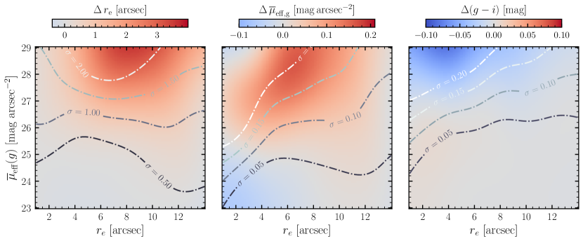
Figure 4: Measurement bias (defined as “truth $-$ measurement”) and uncertainty as a function of the measured angular size $r_{e}$ and surface brightness $\overline{\mu}_{\mathrm{eff}}(g)$. The colors show the bias term while the dashed contours show the constant uncertainty lines. We derive the bias in the total magnitudes from the combined bias in $r_{e}$, $\overline{\mu}_{\mathrm{eff}}(g)$, and color. We find that the bias and uncertainty in our measurement increase toward the fainter end. We apply the bias correction to the real LSBGs before studying their physical properties.

The size, magnitude, surface brightness, and shape of LSBGs are hard to characterize because of their low-surface-brightness nature. We characterize the quality of the structural measurements by comparing the Spergel modeling results with the ground truth for mock Sérsic galaxies. We find that the measured effective radius $r_{e}$ tends to be smaller than the truth, and the bias depends on the surface brightness and the angular size. For surface brightness fainter than $>27\ \mathrm{mag\ arcsec}^{-2}$, the measured size can be much smaller than the truth. As a result, the measured total magnitude $m$ is also too faint. For the measured average surface brightness $\overline{\mu}_{\rm eff}$, the trade-off between the total magnitude and size makes it less biased than the total magnitude. Similar to Zaritsky et al. (2021), we derive the measurement bias and uncertainties in size, surface brightness, total magnitude, and color as a function of size and surface brightness. We refer interested readers to Appendix D for details. The main results are summarized in Figure 4, where the colors show the bias terms as a function of the measured size and surface brightness. The size and surface brightness bias grow with increasing surface brightness. The bias term is not a monotonic function of the size because the size here in Figure 4 is not intrinsic. It is the bias in size measurement that makes galaxies with large intrinsic size pile up around $r_{e}\sim 6\arcsec$. We find the bias in $g-i$ color to be quite small. The $1\sigma$ measurement errors $\sigma(X)$ are shown in Figure 4 as contours, and they have the same units as the bias. We set the minimum uncertainties to be $\sigma(r_{e})\geqslant 0\farcs 3,\ \sigma(\overline{\mu}_{\rm eff})\geqslant 0.05\ \mathrm{mag\ arcsec}^{-2},\ \sigma(g-i)\geqslant 0.05$ to avoid meaninglessly small uncertainties.

We apply the bias corrections to the real LSBGs, estimate the measurement uncertainties, and evaluate the completeness based on the bias-corrected properties. The values presented in our catalogs (Table 3) are already bias-corrected, but we do provide the bias values for reference.

Table 3: UDG and UPG Catalog Description

Column Name	Unit	Description
Type		Galaxy type
ID		Unique LSBG ID
R.A.	deg	Source R.A. in decimal degrees
		(J2000)
Decl.	deg	Source Decl. in decimal degrees
		(J2000)
$r_{e}$	arcsec	Circularized effective radius
$\sigma(r_{e})$	arcsec	Uncertainty in $r_{e}$
$\overline{\mu}_{\mathrm{eff}}(g)$	$\mathrm{mag\ arcsec}^{-2}$	$g$-band average surface brightness
		within $r_{e}$
$\sigma(\overline{\mu}_{\mathrm{eff}}(g))$	$\mathrm{mag\ arcsec}^{-2}$	Uncertainty in $\overline{\mu}_{\mathrm{eff}}(g)$
$m_{g}$	mag	$g$-band apparent magnitude
$\sigma(m_{g})$	mag	Uncertainty in $m_{g}$
$g-i$	mag	$g-i$ color
$\sigma(g-i)$	mag	Uncertainty of $g-i$ color
$g-r$	mag	$g-r$ color
$\sigma(g-r)$	mag	Uncertainty of $g-r$ color
$\nu$		Spergel index
$\varepsilon$		Ellipticity
$A_{g}$	mag	$g$-band Galactic extinction
$A_{r}$	mag	$r$-band Galactic extinction
$A_{i}$	mag	$i$-band Galactic extinction
comp		Completeness
weight		Importance weight
$r_{e,\rm phys}$	kpc	Circularized physical effective radius
$\log\,M_{\star}$	$M_{\odot}$	log stellar mass
$\sigma(\log\,M_{\star})$	$M_{\odot}$	Uncertainty in $\log\,M_{\star}$
host_name		Host galaxy name
host_ra	deg	Host galaxy R.A. in decimal degrees
		(J2000)
host_dec	deg	Host galaxy Decl. in decimal degrees
		(J2000)
host_z		Host galaxy redshift
host_log_m_star	$M_{\odot}$	Host galaxy log10 stellar mass
host_r_vir	kpc	Host galaxy virial radius
host_g_i	mag	Host galaxy $g-i$ color
sep_to_host	arcmin	Angular separation between
		host and UDG/UPG

Note. — The table is published in its entirety in machine-readable format. Magnitudes are on the AB system and have been corrected for measurement biases and Galactic extinction. The information on the host galaxies is from NASA-Sloan Atlas. We provide Galactic extinction corrections, which are derived from the Schlafly & Finkbeiner (2011) recalibration of the Schlegel et al. (1998) dust maps.

4 Mass–Size Outliers Around Milky Way Analogs

The goal of this paper is to study the mass–size outliers in the satellite systems of MW-like galaxies. However, distance information is needed to convert the observed size and magnitude to the physical size and stellar mass. It is well-known that getting the distances to LSBGs is one of the major obstacles to studying their properties. Besides direct distance measurements (e.g., SAGA and ELVES; Kadowaki et al. 2021), it is common to assume a distance to an LSBG by associating it with a host galaxy based on the projected angular distance (e.g., van Dokkum et al., 2015; van der Burg et al., 2016; Wang et al., 2021; Zaritsky et al., 2022; Nashimoto et al., 2022). Statistical background subtraction is then needed to account for the contribution from background and foreground sources. Furthermore, the cross-correlation between an LSBG sample and a host galaxy sample can also reveal the distance distribution of LSBGs (Greene et al., 2022). These methods are also complemented by recent machine-learning techniques (Baxter et al., 2021; Wu et al., 2022).

In this section, we cross-match our LSBG catalog with MW-like galaxies in the NSA catalog. For the LSBGs matched with MW analogs, we run the deblending step to exclude false positives (§3.2) and then run Spergel modeling to measure the properties of LSBGs (§3.3). In the end, we construct the samples of mass–size outliers among the satellites of MW analogs. Table 1 summarizes the number of objects after each step.

4.1 Matching with Milky Way Analogs

The properties of the Milky Way itself vary in the literature (Licquia & Newman, 2015; Bland-Hawthorn & Gerhard, 2016), and the definitions of MW analogs vary between studies. In the SAGA survey (Geha et al., 2017; Mao et al., 2021), MW analogs are selected based on the absolute $K$-band magnitude $-23>M_{K}>-24.6$ mag (corresponding to a stellar mass range of $10.2<\log\,M_{\star}/M_{\odot}<11.0$) and redshift $0.005<z<0.01$ (20–40 Mpc). SAGA generally requires that the MW analogs be in isolation (without nearby bright galaxies). In the ELVES survey (Carlsten et al., 2021, 2022b, 2022a), the requirements for a MW-like host are loosened to be $M_{K}<-22.1$ mag ($M_{\star}>10^{9.9}\ M_{\odot}$) because the probed volume by ELVES ($D<12$ Mpc) is smaller than that of SAGA. In this work, we choose the stellar mass range of our MW analog sample to be $10.2<\log\,M_{\star}/M_{\odot}<11.2$ based on NSA stellar mass, which is simply a 1 dex bin centered at the measured stellar mass of the Milky Way ($M_{\star,\mathrm{MW}}\approx 10^{10.7}\ M_{\odot}$, Licquia & Newman 2015). MW analogs selected using this definition are very close to those in SAGA but are slightly less massive than the ELVES hosts as ELVES has several groups more massive than SAGA hosts. We do not discriminate between isolated or paired hosts. We acknowledge that defining MW analogs is tricky because of the steep mass function of galaxies and limited survey volumes. A slight change in the mass range could alter the number of MW analogs, and how the galaxies populate the brighter end of mass function also matters (see Carlsten et al. 2022a). For example, it is also possible to select MW analogs in linear stellar mass such as $1.5\times 10^{10}<M_{\star}<8.5\times 10^{10}\,M_{\odot}$. Compared to our logarithmic selection, such a linear selection excludes 10% of high-mass MW analogs at $10.9<\log M_{\star}/M_{\odot}<11.2$, and will result in lower abundances of UDGs and UPGs. Better ways to define MW analogs are needed and will certainly benefit the community.

Mass–size outliers, by definition, are relatively scarce compared with “normal” satellites around MW analogs (Mao et al., 2021; Carlsten et al., 2022a). It is therefore helpful to probe a larger volume to obtain better statistics. We choose our redshift range to be $0.01<z<0.04$, which ensures that we can detect a significant number of LSB satellite candidates around MW-like hosts. The depth of HSC limits our detection to below $z\approx 0.04$ because dwarf galaxies will be too small and too faint to be detected beyond that distance. Our search only includes objects larger than $r_{e}\approx 2\arcsec$, which corresponds to $M_{\star}\sim 10^{8.5}\ M_{\odot}$ at $z=0.04$ assuming the average mass–size relation from Carlsten et al. (2021). We also exclude galaxies at $z<0.01$ because (1) the number of mass–size outliers will be very small due to the small volume; (2) their large angular size makes them more vulnerable to being shredded during detection, so including them will introduce a number of spurious LSB objects.

After applying the stellar mass and redshift cuts to the NSA catalog (§2), there are 23,218 MW-like galaxies. We then select those within the HSC PDR2 footprint and match them to the initial LSBG sample (described in §3.1, before the deblending step) as follows.

For a given MW-like galaxy, we calculate its virial mass based on the stellar-to-halo mass relation (SHMR) in Behroozi et al. (2010) using halotools (Hearin et al., 2017). The viral mass is defined to be the enclosed mass with $\rho>\Delta_{\rm vir}(z)\rho_{c}(z)$, where the virial overdensity only depends on cosmological parameters and redshift (Bryan & Norman, 1998). Then we convert virial mass to virial radius $R_{\rm vir}$ using the virial overdensity. It turns out that 40% of our hosts have virial radii larger than 300 kpc, which is commonly used for the virial radius of the Milky Way. We note that the SHMR from abundance matching might overestimate the halo mass for massive spirals (e.g., Posti et al., 2019; Mancera Piña et al., 2022a), implying that our sample might include LSBGs beyond the virial radius. We also compare different SHMRs (e.g., Moster et al., 2013) and do not find significant differences in the distribution of $R_{\rm vir}$.

Then we identify any LSBG that falls inside the projected virial radius of a host. About 40% of LSBGs are matched with 2 hosts and about 15% of them are matched with 3 or more hosts. If an LSBG is matched to multiple hosts, we assign it to the nearest host based on the separation normalized by the host virial radius. There are 922 MW-like hosts and 10,579 LSBG candidates associated with them. These MW analogs occupy a sky area of 89.19 deg² (out to $1\ R_{\rm vir}$).

As described in §3.2, we perform a deblending step to effectively remove spurious objects. There are 2673 objects left after the deblending cuts. Next, we model these remaining objects using the Spergel profile as described in §3.3 and obtain their photometry and structural parameters from the best-fit models. We also remove duplicate objects. In the final catalog, we are left with 2510 LSBG candidates associated with 689 MW analogs (out of 922) as our final LSBG sample. The host number drops from 922 to 689 because many hosts in the prior sample have no true positives as their satellites. We note that these LSBGs are matched to MW hosts in projection but do not have direct distance measurements, and we have not applied any statistical background correction at this stage.

We apply the measurement bias correction (§3.4) and assign completeness after bias correction. Lastly, we correct for the effect of Galactic extinction on colors based on Schlegel et al. (1998) and Schlafly & Finkbeiner (2011). The stellar masses of cross-matched LSBG are derived from the Spergel model fitting and the relation between color and mass-to-light ratio $M_{\star}/L$ from Into & Portinari (2013):

$$\log\left(M_{\star}/L_{g}\right)=1.774\,(g-r)-0.783,$$

$$\log\left(M_{\star}/L_{g}\right)=1.297\,(g-i)-0.855.$$

Kado-Fong et al. (2022) show that the UDG population can be well described by the color–$M_{\star}/L$ relation from Into & Portinari (2013), which is also used in ELVES (Carlsten et al., 2022a). We note that the stellar mass derived using the color–$M_{\star}/L$ relation from Herrmann et al. (2016) and Du et al. (2020) is $\sim 0.2$ dex lower than the one derived using the Into & Portinari (2013) relation. In our case, because we have both the $g-r$ and $g-i$ colors available from the model fitting, we use the average $M_{\star}/L$ derived from the two colors to calculate stellar mass. We assume the solar absolute magnitude in the $g$ band to be 5.03 (Willmer, 2018).

4.2 Mass–Size Outlier Sample

The concept of UDG was proposed to describe galaxies with unusually large sizes ($r_{e}>1.5$ kpc) and low central surface brightnesses ($\mu_{0}(g)>24.0\ \mathrm{mag\ arcsec}^{-2}$; van Dokkum et al. 2015). Although UDGs are large in size, the constant size cut does not account for the fact that the galaxy size is strongly correlated with its mass, known as the mass–size relation (e.g., Graham & Guzmán, 2003; Trujillo et al., 2007; van Dokkum et al., 2013; Cappellari, 2013; Lange et al., 2015). For example, a galaxy with $r_{e}=1.5$ kpc is very extended if its stellar mass is $10^{7}\ M_{\odot}$, but is normal-sized if its stellar mass is $10^{8.5}\ M_{\odot}$. Thus, a more physically useful definition of puffy dwarf galaxies (i.e., mass–size outliers) would be based on a mass–size relation and its scatter. Following this thread, we propose a new definition of mass–size outliers, dubbed ultra-puffy galaxies (UPGs).

It is worth noting that in several works (e.g., Lim et al., 2020; Venhola et al., 2022), UDGs in galaxy clusters are defined as outliers in the scaling relations between size, surface brightness, and total luminosity. A UDG definition based on the mass–size relation is also used in simulation studies where the absolute sizes were uniformly too large such that size outliers could only be selected relative to the simulated mass–size relation (e.g., Benavides et al., 2021, 2022). In this work, we are proposing such a definition of mass–size outliers to be used universally, not limited to cluster environments or simulations.

In this section, we describe the definition of UPG and contrast it with UDG. Then we select UDGs and UPGs from our LSBGs matched with MW hosts. The catalogs and mosaic images of UDGs and UPGs are available online.

4.2.1 UPGs

To select mass–size outliers, a mass–size relation and its scatter are needed. In general, the slope of the mass–size relation in the nearby Universe has been shown to be color- and morphology-dependent for galaxies above $M_{\star}>10^{9}\ M_{\odot}$: blue star-forming galaxies have a shallower mass–size relation than do red quenched galaxies (e.g., Lange et al., 2015). In the dwarf galaxy regime ($10^{5.5}<M_{\star}/M_{\odot}<10^{8.5}$), Carlsten et al. (2021) derive the mass–size relation from the satellites of MW analogs in the Local Volume and show that the average mass–size relation is quite universal: the slope and intercept are not sensitive to the color or morphology of dwarf galaxies. Residuals from the mass–size relation follow a log-normal distribution reasonably well. This fact allows us to define a subset of dwarf galaxies that are outliers with respect to the average mass–size relation.

Taking the measured average mass–size relation from Carlsten et al. (2021) $\log\,(r_{e}/\mathrm{pc})=0.25\,\log\,(M_{\star}/M_{\odot})+1.07$ and a scatter of $\sigma=0.18$ dex, we define a population of UPGs to be galaxies that are $>1.5\sigma$ above the average mass–size relation. We note that the mass–size relation in Carlsten et al. (2021) is derived for a mass range of $10^{5.5}\ M_{\odot}<M_{\star}<10^{8.5}\ M_{\odot}$, so the mass–size relation is extrapolated to $M_{\star}\sim 10^{9}\ M_{\odot}$ to define our UPG sample. We choose $1.5\sigma$ because it gives us a statistically significant sample. One can certainly select $>2\sigma$ or $>3\sigma$ UPGs if a larger LSBG sample is available. The UPGs are not absolutely large in size or absolutely faint in surface brightness, but they are outliers in size for their stellar masses. For example, a UPG with $M_{\star}=10^{7}\ M_{\odot}$ has a size larger than 1.2 kpc and surface brightness fainter than $\overline{\mu}_{\mathrm{eff}}(g)>25.5\ \mathrm{mag\ arcsec}^{-2}$ for $g-i=0.4$ and $\overline{\mu}_{\mathrm{eff}}(g)>26.8\ \mathrm{mag\ arcsec}^{-2}$ for $g-i=0.8$. A UPG with $M_{\star}=10^{8.5}\ M_{\odot}$ has a size larger than 2.7 kpc and surface brightness fainter than $\overline{\mu}_{\mathrm{eff}}(g)>23.7\ \mathrm{mag\ arcsec}^{-2}$ for $g-i=0.4$ and $\overline{\mu}_{\mathrm{eff}}(g)>25.0\ \mathrm{mag\ arcsec}^{-2}$ for $g-i=0.8$. The definition of UPG based on the observed mass–size relation is physically motivated, and better allows us to study size outliers at a given stellar mass. We further discuss the advantages and disadvantages of UDG and UPG in §5.1 and §6.

There are 362 LSBG candidates that fall $1.5\sigma$ above the ridge line of the mass–size relation. After removing spurious objects (e.g., shredded galaxy outskirts, cirrus, tidal feature, blends) by another round of visual inspection and removing objects with completeness less than 0.1, we have 337 galaxies in our UPG sample. These UPGs are associated with 239 hosts. The total sky area occupied by UPG hosts (out to 1 $R_{\rm{vir}}$) is 32.37 deg². The catalogs are available online in machine-readable format, and we demonstrate the catalog format in Table 3.

4.2.2 UDGs

We also select a UDG sample from our LSBGs in order to compare it with existing observations and simulations in different environments. The UDG sample is usually defined based on the surface brightness and physical size of the galaxy. However, there are many different criteria in the literature: van Dokkum et al. (2015) define UDGs to have effective radii $r_{e}$ larger than 1.5 kpc and central surface brightness $\mu_{0}(g)$ fainter than $24.0\ \mathrm{mag\ arcsec}^{-2}$; other groups also use the surface brightness at $r_{e}$ (e.g., Di Cintio et al., 2017; Cardona-Barrero et al., 2020) or the average surface brightness within $r_{e}$ to define UDGs (e.g., Koda et al., 2015; Yagi et al., 2016; van der Burg et al., 2016; Leisman et al., 2017; Mancera Piña et al., 2018, 2019a; Martin et al., 2019; Karunakaran & Zaritsky, 2022). The size criterion also varies from $r_{e}>1$ kpc to $r_{e}>1.5$ kpc. Van Nest et al. (2022) explore these definitions in simulations and find that different definitions of “UDG” can drastically change the selected subset of dwarfs, therefore affecting our understanding of the UDG population.

In practice, the measured central surface brightness might be biased by nuclear star clusters (Neumayer et al., 2020; Carlsten et al., 2022b; Somalwar et al., 2020) or other contaminants. Therefore in this work, we use the average surface brightness within the effective radius $\overline{\mu}_{\mathrm{eff}}(g)$ to define UDGs. The difference between the average surface brightness and the central surface brightness can be analytically calculated for a Sérsic profile: $\overline{\mu}_{\mathrm{eff}}-\mu_{0}=1.124$ for $n=1$ and 0.796 for $n=0.8$ (Graham & Driver, 2005; Yagi et al., 2016). As dwarf galaxies and UDGs typically have Sérsic indices of $0.8<n<1.2$ (e.g., van Dokkum et al., 2015; Carlsten et al., 2021), we take $\overline{\mu}_{\mathrm{eff}}-\mu_{0}=1.0$ as an average value to convert $\mu_{0}$ to $\mu_{\mathrm{eff}}$. In this work, we define UDGs to be galaxies with $r_{e}+\sigma(r_{e})>1.5$ kpc and $\overline{\mu}_{\mathrm{eff}}(g)+\sigma(\overline{\mu}_{\mathrm{eff}}(g))>25\ \mathrm{mag\ arcsec}^{-2}$ to take the $1\sigma$ measurement errors into account. As a result, there are a few objects with nominally smaller sizes but large uncertainties that scatter into our UDG sample. This definition maximizes the consistency with the definition in van Dokkum et al. (2015) while not losing UDGs harboring nuclear star clusters.

Among the 2510 LSBG candidates around MW analogs, there are 432 objects satisfying the UDG definition. We did a final visual inspection for these objects and excluded 16 objects that are false positives including blends and Galactic cirrus. We also removed another 4 objects having completeness less than 0.1. In the end, we obtained our UDG sample with 412 objects (associated with 258 hosts) after searching around 689 MW analogs. The total sky area occupied by UDG hosts (out to 1 $R_{\rm{vir}}$) is 32.71 deg². We describe the properties of the mass–size outliers (including UPGs and UDGs) in §5.1.

4.3 Background Contamination Fraction

Although we have matched LSBGs to MW analogs by proximity in projection, the physical affiliation of LSBGs to the host is not guaranteed. As a result, a certain fraction of galaxies in our mass–size outlier samples are foreground or background galaxies that fall within the virial radius of the host by chance. Given the volume and the surface brightness range of our search, contamination is most likely to be dominated by background galaxies. In this section, we try to estimate the contamination fraction empirically by randomly matching LSBGs to our MW hosts and measuring the number density of apparent UPGs and UDGs.

We randomly selected a continuous patch of sky of 24 deg² in HSC PDR2 regardless of whether it contains MW analogs. Then we performed the same deblending and modeling steps for the 2707 LSBG candidates detected in this region. We also removed objects that are already in our mass–size outlier samples and objects with completeness less than 0.1. We also did the same visual inspection as for UDGs and UPGs to remove false positives. In the end, we obtained 480 LSBGs (excluding false positives) representing a population of possible contaminants for the UDG and UPG samples. Next, because both UDG and UPG are defined based on the physical size, we randomly associated the 480 LSBGs with the 922 MW analogs that are surveyed in this paper. Then we calculated a physical size for each LSBG and classify an LSBG as an “artificial“ UDG or UPG if it satisfied the corresponding definition. We repeated such random matching 200 times. In the end, we obtained 7,625 artificial UDGs and 8267 artificial UPGs. These UDGs and UPGs are “artificial” only in the sense of being artificially associated with random MW hosts.

In this way, the number density of artificial UDGs is estimated to be $S_{\rm UDG}=1.60\pm 0.25\ \mathrm{deg}^{-2}$, and the number density of artificial UPGs is $S_{\rm UPG}=1.72\pm 0.23\ \mathrm{deg}^{-2}$. The catalogs of artificial UDG and UPGs are also available online. Using the number densities and the probed area of our survey (89.19 deg² occupied by 922 hosts), we calculate the contamination fraction for both the UDG and UPG samples. For the UDG sample, we find $f_{\rm contam}^{\rm UDG}\approx 35\%\pm 5\%$; for the UPG sample, the contamination fraction is $f_{\rm contam}^{\rm UPG}\approx 45\%\pm 6\%$. We take the contamination fraction into account when calculating the abundances in §5.

5 Results

In this section, we compare the distributions of UDGs and UPGs on the size–surface brightness and mass–size planes to gain intuition on the differences between UDG and UPG definitions. Then we present the abundances of UDGs and UPGs and compare them with the literature.

5.1 Properties of Mass–Size Outliers

Figure 5: Left panel: schematic diagram showing the UDG size cut (gray band), survey limit (blue shade), average mass–size relation (dark green dashed line), and $1.5\sigma$ above it (light green line). The solid lines are constant surface brightness cuts at $\overline{\mu}_{\mathrm{eff}}(g)=25\ \mathrm{mag\ arcsec}^{-2}$ for two different colors $g-i=0.4$ (blue) and $g-i=0.8$ (red). The constant surface stellar mass density line is in purple, which is parallel to the solid lines. The dotted part of the green lines indicates where we linearly extrapolate the mass–size relation to define UPGs. Right panel: distributions of UDGs and UPGs on the mass–size plane. UDGs that are also classified as UPGs are shown as orange squares, while UDGs that do not satisfy the UPG definition are marked as red stars. Conversely, blue triangles are UPGs that are not classified as UDGs. The UDG sample includes a significant number of galaxies that are not mass–size outliers (falling below the $1.5\sigma$ line), which are red in color because the surface brightness cuts are different on the mass–size plane for blue and red galaxies.

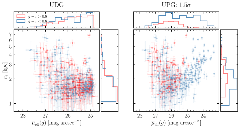
Figure 6: Distribution of UDGs (left) and UPGs (right) on the size–surface brightness plane. The UPGs are defined to be galaxies that are $1.5\sigma$ above the average mass–size relation in Carlsten et al. (2021). The samples are split into two color bins and shown in red ($g-i>0.8$) and blue ($g-i<0.8$). The marginal histograms are not normalized to highlight the relative number of red and blue galaxies. Compared with the UDG sample, the UPG sample includes blue galaxies with surface brightness higher than the UDG cut ($\overline{\mu}_{\mathrm{eff}}(g)<25\ \mathrm{mag\ arcsec}^{-2}$) and excludes red galaxies at $25<\overline{\mu}_{\mathrm{eff}}(g)<26\ \mathrm{mag\ arcsec}^{-2}$, due to the color–$M_{\star}/L$ dependence.

We show UDGs and UPGs on the mass–size plane in Figure 5. To orient the reader to the mass–size plane, we first show a schematic diagram in the left panel where regions relevant to the definitions of UDG and UPG are highlighted. The light blue shade shows the survey limit; we cannot effectively probe LSBGs fainter than $\overline{\mu}_{\mathrm{eff}}(g)\gtrsim 27.5\ \mathrm{mag\ arcsec}^{-2}$ (see §3.4). For defining UDGs, a physical size cut and a surface brightness cut are needed. We show the $r_{e}=1.5$ kpc cut as a horizontal gray band (spanning from 1.1 to 1.5 kpc) to acknowledge the fact that smaller galaxies with large size uncertainties are included in the UDG sample. The slanted solid lines show constant surface brightness lines with $\overline{\mu}_{\mathrm{eff}}(g)=25.0\ \mathrm{mag\ arcsec}^{-2}$ for two different colors ($g-i=0.4$ and $g-i=0.8$). For our redshift range, the cosmological dimming effect is negligible and the surface brightness is constant with distance. The constant surface brightness lines depend on color because of the color–$M_{\star}/L$ relation. We also show the constant surface stellar mass density ($\mu_{\star}$) line, which is parallel to the constant surface brightness lines because the surface mass density is proportional to surface brightness multiplied by the mass-to-light ratio. Therefore, at a given size and surface brightness, blue UDGs are less massive than red UDGs; at a given stellar mass and surface brightness, blue UDGs are larger than red UDGs in size. Such a constant surface brightness cut leads to a UDG population that is inhomogeneous in surface mass density.

In the left panel of Figure 5, the green dashed lines show the average mass–size relation and the $1.5\sigma$ line above the average relation. UPGs would lie above the $1.5\sigma$ line by construction, and there will be an overlap between UDGs and UPGs. The mass–size relation is shallower than the constant surface brightness and surface mass density lines.

We highlight the similarities and differences between the UDGs and UPGs in the right panel. UDGs that are also classified as UPGs are shown as orange squares, whereas UDGs that do not satisfy the UPG definition are marked as red stars. Blue triangles correspond to UPGs that are not classified as UDGs. Limited by the detection limit and the fact that our hosts lie beyond the Local Volume, our mass limit is $M_{\star}\approx 10^{6.5}\ M_{\odot}$, which is $\sim 1$ dex higher than ELVES. Compared with the UPG sample, we find that the UDG sample (orange squares + red stars) comprises a number of galaxies below the $1.5\sigma$ line, but also loses several low-mass galaxies that are above the $1.5\sigma$ line but have sizes smaller than 1.5 kpc. For the UDG sample, the stellar mass range only reaches $M_{\star}\approx 10^{8.3}\ M_{\odot}$ because galaxies with higher stellar mass are too bright to satisfy the UDG surface brightness criterion. On the contrary, as the UPG definition does not have a hard surface brightness cut, it includes many galaxies that are more massive than UDGs provided they have an extraordinarily large size. We also note that the mass–size relation from Carlsten et al. (2021) is extrapolated to define UPGs in the mass range $10^{8.5}\ M_{\odot}<M_{\star}<10^{9}\ M_{\odot}$, where about 10% of our UPGs are located (dotted green lines in Figure 5). However, the mass–size relation might show color and morphology dependence for $M_{\odot}>10^{8.5}\ M_{\odot}$. As a consequence, disk galaxies might contribute to the UPG sample at the high-mass end. We visually checked the UPG sample and did find some blue UPGs resembling disk galaxies at the high-mass end. A spectroscopic follow-up would be required to confirm whether they are just blue background galaxies. We also note that 7% of our UDGs and 3% of our UPGs have Sérsic indices $n>1.5$. We believe these galaxies with large Sérsic indices are mostly interlopers given the fact that $\sim$40% of UDGs and UPGs are interlopers (see §4.3). We do not consider these galaxies to derive our conclusions given their small contribution to the whole sample.

We also show the UDG and UPG samples on the size–surface brightness plane in Figure 6. The galaxies are split into two color bins and are shown in blue ($g-i<0.8$) and red ($g-i>0.8$), respectively. We do not apply any background contamination correction in Figure 6 because such corrections can only be done in a statistical sense. The error bars correspond to $1\sigma$ measurement uncertainties (§3.4). The two marginal plots show the unnormalized histograms of galaxies in the two color bins. The numbers of red and blue galaxies are similar in the UDG sample, but there are more blue galaxies than red ones in the UPG sample. As there is no hard surface brightness cut for UPGs, the UPG sample includes many blue galaxies with brighter surface brightness ($23\lesssim\overline{\mu}_{\mathrm{eff}}(g)<25\ \mathrm{mag\ arcsec}^{-2}$). For blue UPGs (shown as blue dots), the apparent correlation between $\overline{\mu}_{\mathrm{eff}}(g)$ and $r_{e}$ is merely due to the fact that blue UPGs pile up around the $1.5\sigma$ line above the mass–size relation. Due to the surface brightness cut ($\overline{\mu}_{\mathrm{eff}}(g)>23.0\ \mathrm{mag\ arcsec}^{-2}$) in the deblending step, there is little chance for an LSB disk galaxy with a bright bulge to scatter into the UPG sample. The UPG sample also loses a significant fraction of red galaxies at $25<\overline{\mu}_{\mathrm{eff}}(g)<26\ \mathrm{mag\ arcsec}^{-2}$ because their stellar masses are high but their sizes are too small to be mass–size outliers (i.e., red stars in Figure 5).

5.2 Abundance of Mass–Size Outliers

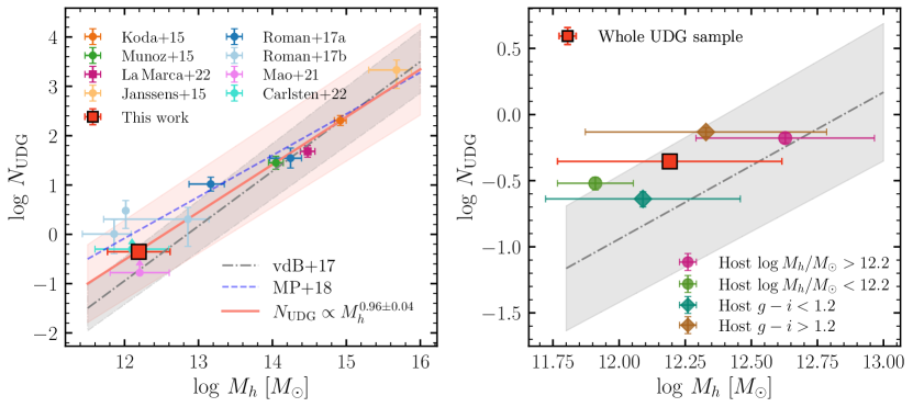
Figure 7: Abundance of UDGs as a function of the host halo mass. Left: We compile the UDG abundance measurements from the literature covering a wide range of host mass. The UDG abundance from our work $N_{\rm UDG}=0.44\pm 0.05$ is shown as a red square, and the power-law relations from van der Burg et al. (2017) and Mancera Piña et al. (2018) are shown in gray and blue respectively. Our fitting result is shown in pink. Our UDG abundance is consistent with ELVES but significantly higher than that in SAGA. After including more measurements at the lower halo-mass end, the power law is shallower than the relation reported in van der Burg et al. (2017). Right: We split the UDG sample into bins based on the host halo mass (circles) and $g-i$ color (diamonds). The UDG abundance is higher for more massive hosts and redder hosts.

As demonstrated by many previous studies (e.g., van der Burg et al., 2016, 2017; Román & Trujillo, 2017b; Karunakaran & Zaritsky, 2022), the average number of UDGs per host scales with host halo mass. While much literature focuses on finding UDGs in clusters and large groups, there are fewer constraints on the UDG abundance at the lower halo-mass end. In this section, we calculate the UDG and UPG abundances of MW analogs and compare them with other surveys.

We define the UDG (UPG) abundance as the average number of UDGs (UPGs) per host galaxy. We searched 922 MW analogs. In our UDG sample, there are 412 UDGs associated with 258 hosts. After correcting for background contamination (see §4.3) and completeness (see §3.4), the UDG abundance of MW analogs is $N_{\rm UDG}=0.44\pm 0.05$ per host. The UPG abundance in our sample is $N_{\rm UPG}=0.31\pm 0.04$ per host. Here we neglect the fact that the number of satellites contained within the virial sphere is different from the number of satellites within a projected cylinder with virial radius (the so-called deprojection factor; van der Burg et al. 2017).

We compare our UDG abundance with other surveys focused on MW analogs. In the SAGA survey (Mao et al., 2021), 6 satellite galaxies (out of 127 spectroscopy-confirmed satellites around 36 MW analogs) satisfy the definition of UDG. Therefore the UDG abundance in Mao et al. (2021) is about $N_{\rm UDG}^{\rm SAGA}\approx 0.17\pm 0.07$. In the ELVES survey (Carlsten et al., 2022a), there are 13 UDGs out of 351 satellites with secure distances ($P_{\rm sat}>0.8$) in 30 MW analogs, leading to a UDG abundance of $N_{\rm UDG}^{\rm ELVES}\approx 0.43\pm 0.12$. If we only take UDGs more massive than our detection limit $M_{\star}>10^{6.5}\ M_{\odot}$, we obtain slightly lower UDG abundances of $N_{\rm UDG,6.5}^{\rm ELVES}\approx 0.36\pm 0.11$. Because both SAGA and ELVES select satellites based on distance measurements and do not correct for completeness, we interpret their UDG abundances as lower limits. Román & Trujillo (2017a) identified 11 UDGs around three galaxy groups in the IAC Stripe 82 Legacy Survey (Fliri & Trujillo, 2016), but it is hard to calculate a UDG abundance due to small-number statistics. Our UDG abundance is consistent with the value in the ELVES survey, but higher than the value from SAGA. This might be explained by the different photometric depths of data used. As pointed out by Carlsten et al. (2022a) and Font et al. (2022), the SAGA survey reaches a surface brightness depth of $\overline{\mu}_{\mathrm{eff}}(r)\approx 25\ \mathrm{mag\ arcsec}^{-2}$, which is $\sim 2.5\ \mathrm{mag\ arcsec}^{-2}$ shallower than the ELVES survey and this work. It is probable that SAGA missed some fraction of red and lower surface brightness galaxies. On the other hand, ELVES includes several more massive hosts than our search and SAGA do, and consequently bias the UDG abundance.

We plot the UDG abundances from these surveys in the left panel of Figure 7, together with the results for larger galaxy groups and clusters (Koda et al., 2015; Muñoz et al., 2015; Román & Trujillo, 2017b, a; Janssens et al., 2017; van der Burg et al., 2017; La Marca et al., 2022). The power-law regression result from van der Burg et al. (2017) $N_{\rm UDG}\propto M_{h}^{1.11\pm 0.07}$ is shown in gray. We also show the result from Mancera Piña et al. (2018) $N_{\rm UDG}\propto M_{h}^{0.84\pm 0.07}$ as a blue-dashed line where they homogeneously combined the samples in van der Burg et al. (2016) and Román & Trujillo (2017a). The UDG abundance of this work is highlighted as the red square. As shown in Figure 7, the scatter in the $N_{\rm UDG}-M_{h}$ relation gets larger at the lower halo-mass end, but this might be due to the small statistics in prior studies and the differences in completeness. Our UDG abundance is marginally higher than the prediction from van der Burg et al. (2017) but is still consistent considering the large scatter of the power law.

Taking all data points from the literature (as shown in Figure 7), we use the orthogonal distance regression (ODR) to fit a power-law between $N_{\rm UDG}$ and host halo mass $M_{h}$ and find $N_{\rm UDG}\propto M_{h}^{0.96\pm 0.04}$, shown as the red solid line in Figure 7. The slope of the power law is shallower than van der Burg et al. (2017) ($\beta=1.11\pm 0.07$) but steeper than Román & Trujillo (2017a) ($\beta=0.85\pm 0.05$). Mancera Piña et al. (2018) surveyed eight clusters and find a sublinear power law. Recently Karunakaran & Zaritsky (2022) performed a similar analysis including SAGA, ELVES, and Nashimoto et al. (2022) and found a slightly shallower power law of $\beta=0.87\pm 0.07$. We note that their surface brightness cut for UDGs is brighter than ours and thus they include more “UDGs” for MW-like hosts and have a shallower power law. One should be aware of the fact that literature results are of different depths, often not completeness corrected and background subtracted, and UDG definitions also vary across different studies. These effects could significantly bias the results when combining them. Therefore we caution that the UDG abundance and the power-law index here should not be over-interpreted.

In the right panel of Figure 7, we split the UDG sample into different bins based on their host halo mass (shown as circles) and host color (shown as diamonds). We find that the UDG abundance is slightly higher for hosts with higher halo mass and redder color, but the trend is stronger with host color.

Because there is little literature on UPGs, we only compare our UPG abundance with ELVES. In ELVES, we take the 351 satellites with secure distances in 30 MW analogs and identify 36 UPGs associated with 20 hosts. Thus the UPG abundance fraction in ELVES is $N_{\rm UPG}^{\rm ELVES}=1.20\pm 0.20$. When only selecting UPGs with $M_{\star}>10^{6.5}\ M_{\odot}$, we obtain 23 UPGs in 30 MW analogs, thus $N_{\rm UPG,6.5}^{\rm ELVES}=0.77\pm 0.16$, which is slightly higher than our UPG abundance.

Another interesting quantity is the fraction of satellites that are mass–size outliers in a group or cluster. This fraction represents how efficient an environment is at producing puffy satellites. We denote this quantity as the UDG (UPG) fraction hereafter, which characterizes the tail of the size distribution of satellites. In order to calculate this fraction, we assume that MW analogs have $\sim 6\pm 1$ satellites with $M_{\star}>10^{6.5}\ M_{\odot}$ (Carlsten et al., 2022a). This lower limit in stellar mass is roughly our detection limit (see Fig. 5). Then for our samples, the UDG (UPG) fraction is $f_{\rm UDG}\approx 0.07\pm 0.02$ and $f_{\rm UPG}\approx 0.05\pm 0.02$. In ELVES, among 351 satellites with secure distances in 30 MW analogs, we identify 13 UDGs associated with 10 hosts and 36 UPGs associated with 20 hosts. Thus the UDG fraction in ELVES is $f_{\rm UDG}^{\rm ELVES}\approx 0.04\pm 0.01$, the UPG fraction in ELVES is $f_{\rm UPG}^{\rm ELVES}\approx 0.10\pm 0.02$. We further only select ELVES galaxies with $M_{\star}>10^{6.5}\ M_{\odot}$ and find the same UDG and UPG fractions. We also compare our results with results in the Virgo cluster. Taking the data from the Next Generation Virgo Cluster Survey (NGVS; Ferrarese et al. 2020) and only considering satellites with $M_{\star}>10^{6.5}\ M_{\odot}$, there are 14 UDGs and 17 UPGs out of 218 identified satellites (with no completeness correction). Thus their UDG (UPG) fraction is $f_{\rm UDG}^{\rm Virgo}\approx 0.06\pm 0.02$ and $f_{\rm UPG}^{\rm Virgo}\approx 0.08\pm 0.02$. However, we note that Ferrarese et al. (2020) only survey the central 4 deg² of the Virgo cluster, which probably biases the UDG (UPG) fraction. We interpret our UDG and UPG fractions to be consistent with ELVES and NGVS. However, we emphasize that it is challenging to compare across various searches due to the differences in the host sample selection, depth, completeness, and contamination estimation. In the future, a more systematic and careful comparison of UDG (UPG) fractions in different environments is needed.

6 Robust Identification of Mass–Size Outliers

In Figure 5, we find that combining a hard physical size cut with a surface brightness cut carves out an interesting region of the mass–size plane that is complicated in two ways. On the one hand, there are many galaxies classified as UDGs that are not size outliers at $M_{\star}\sim 10^{7.5}\ M_{\odot}$ (highlighted as red stars in Fig. 5). On the other hand, the hard surface brightness cut corresponds to very different surface mass densities between red and blue UDGs, making it hard to directly compare them, as they occupy different regions on the mass–size plane. For a given stellar mass and size (e.g., at $M_{\star}\sim 10^{7.5}\ M_{\odot}$ and $r_{e}=1.5$ kpc), the hard surface brightness cut in the UDG definition preferentially removes blue galaxies because their surface brightnesses are higher and their $M_{\star}/L$ ratios are lower. Thus, red UDGs are over-represented. If one calculates the quenched fraction of UDGs as a function of the stellar mass, it will be biased high because of this constant surface brightness cut in the UDG definition (see Li et al. 2023). These limitations of the original UDG definition are also discussed in Trujillo et al. (2017) and Mancera Piña et al. (2018).

It is worth emphasizing that the concept of UDG was originally proposed in a cluster context (e.g., van Dokkum et al., 2015) where UDGs are far less diverse in stellar populations compared with field UDGs, hence the sample selection suffers less from the effect of color–$M_{\star}/L$ relation. However, UDGs are not all red and quiescent. Blue UDGs are found in less dense environments and fields. Therefore, the concept of UDG might not be optimal for systematic studies outside of a cluster environment; more specifically, to study diffuse dwarf galaxies with a range of colors in different environments, a more stellar-population agnostic criterion must be adopted to select samples. The UPG is defined based on the average mass–size relation and thus alleviates some of the issues in the UDG definition. UPGs are defined to lie $1.5\sigma$ above the average mass–size relation of the satellites in MW analogs in the Local Volume. The specific value above the average mass–size relation can be varied to probe different parts of the size distribution. We advocate studying the UPG population in both observations and simulations to explore samples with different “puffiness” (e.g., comparing UPG at $1.5\sigma$ and $2\sigma$ from the mass–size relation).

Because the UPG is a physically motivated selection, to use the UPG criteria, one needs to know the distance, color, a color–$M_{\star}/L$ relation to convert observed magnitudes to stellar mass, and a mass–size relation and the scatter therein. None of these are easy to obtain or free from systematic errors. Both size and stellar mass could have large uncertainties in the LSB regime. One also needs to apply a surface brightness cut (such as $\overline{\mu}_{\mathrm{eff}}(g)>23.0\ \mathrm{mag\ arcsec}^{-2}$ in this work) to make sure that the UPG sample is not dominated by disk galaxies with high surface brightness due to the bulges. In §4.3, we find that the UPG sample has a higher contamination fraction than the UDG sample. As the UPG definition does not preferentially exclude blue LSBGs, many background disk galaxies can be misidentified as UPGs. Based on our tests, a UPG sample with a more aggressive cut (e.g., $>2\sigma$ above the average mass–size relation) would have a higher purity, but building a significant sample of these is only possible when one has a much larger and deeper LSBG sample.

Our definition of UPG greatly benefits from the well-measured mass–size relation in Carlsten et al. (2021) and the fact that this mass–size relation is independent of galaxy color and morphology. However, such mass–size relations are not always available for all galaxy mass ranges and environments (in the field or in groups and clusters). Carlsten et al. (2021) derive the mass–size relation of satellite galaxies of MW analogs below $M_{\star}\sim 10^{8.5}\ M_{\odot}$, and find it similar to the mass–size relation of field late-type dwarfs in Karachentsev et al. (2013). Lange et al. (2015) have relatively good constraints on the mass–size relation above $M_{\star}\sim 10^{9}\ M_{\odot}$. However, the mass–size relation at $10^{8.5}\ M_{\odot}<M_{\star}<10^{9.5}\ M_{\odot}$ has been shown to be very shallow for red galaxies (Smith Castelli et al., 2008; Misgeld et al., 2008; Misgeld & Hilker, 2011; Eigenthaler et al., 2018), and its dependence on color, morphology, or environment is still unclear. In this work, we simply extrapolate the Carlsten et al. (2021) mass–size relation to $10^{9}\ M_{\odot}$. However, it is not clear whether the mass–size relation at $10^{8.5}\ M_{\odot}<M_{\star}<10^{9}\ M_{\odot}$ is sensitive to color or morphology. Future work should revisit the mass–size relation in this regime.

At the same time, whether the size distribution for a given mass can be well-described by a Gaussian distribution is still a question. Fig. 9 in Carlsten et al. (2021) shows the residual in $\log(r_{e})$ after fitting the mass–size relation, where the distribution of residuals is roughly Gaussian but skewed toward the large-size end. With enough statistics in the future, one might be able to characterize the shape of the large-size tail and define UPGs based on the percentiles of the size distribution (Greene et al., 2022). However, there are also other size definitions that may help reduce the scatter in the mass–size relation (e.g., Miller et al., 2019; Mowla et al., 2019; Trujillo et al., 2020; Chamba et al., 2022) and can further refine the UPG definition proposed in this work.

In the right panel of Figure 5, we also plot the lines of constant average surface mass density, which are steeper than the mass–size relation but have the same slope as constant surface brightness lines. Hence, a possible improvement to the selection of diffuse galaxies could be to select galaxies with low-surface mass density. Similar to the method proposed in this work, this method also alleviates the artifacts introduced by the color–$M_{\star}/L$ relation on the mass–size plane. We defer the exploration of this definition to future work.

7 Summary

In this work, we perform a search for low surface brightness galaxies in HSC PDR2 data and construct samples for mass–size outliers around MW analogs at $0.01<z<0.04$. Besides the UDGs, we define “ultra-puffy galaxies” to be $1.5\sigma$ above the average mass–size relation. We calculate the abundances of mass–size outliers and compare them with literature. We also argue that UPGs better represent the large-size tail of the dwarf galaxy population. Our main findings and prospects are summarized below.

1. Using the HSC PDR2 data ($\sim 300\ \mathrm{deg}^{2}$), we conduct a systematic search for LSBGs using the method in Greco et al. (2018) complemented by our new deblending and modeling methods. Utilizing the nonparametric models generated by scarlet, we design a metric based on morphological parameters to effectively remove false positives in the initial LSBG sample. We measure the structural properties of LSBGs using parametric modeling and carefully characterize the measurement biases and uncertainties. The completeness of the search is also derived by injecting mock galaxies. Our LSBG search achieves high completeness compared with other searches and demonstrates the power of HSC (and future LSST) data for LSB science.

2. By matching LSBGs with MW analogs in the NSA catalog, we construct samples of mass–size outliers including UDGs and UPGs. We display their distributions on the mass–size plane (Figure 5) and the size–surface brightness plane (Figure 6). The UPG sample contains more blue and higher surface brightness galaxies than the UDG sample. In contrast, the UDG sample includes many red galaxies below $1.5\sigma$ from the average mass–size relation.

3. After correcting for background contamination and completeness, the UDG abundance in MW analogs is $N_{\rm UDG}=0.44\pm 0.05$ per host and the UPG abundance is $N_{\rm UPG}=0.31\pm 0.04$ per host. Our UDG abundance agrees with ELVES quite well but is much higher than that in SAGA. We obtain a UPG abundance lower than that in ELVES.

4. Combining data from studies in denser environments, we find that the UDG abundance follows a sublinear power law with the host halo mass. The power-law slope agrees with other studies considering the errors. We caution that each study adopts different UDG definitions and may or may not correct for completeness, which could bias the results.

5. For an MW analog, on average, about $7\%\pm 2\%$ of its satellites are UDGs and about $5\%\pm 2\%$ of its satellites are UPGs. Our UDG and UPG fractions are consistent with ELVES and NGVS.

6. We advocate the concept of UPG, which is physically motivated, does not introduce artifacts in the mass–size distribution, and better represents the large-size tail of dwarf galaxy population.

This paper presents the UDG and UPG sample and explores their abundances. In our Paper II (Li et al., 2023), we study their size and spatial distributions and their star formation status. This study is focused on a small subset of LSBG candidates matched with MW analogs. In future work, we would like to exploit the full sample to study interesting topics on LSBGs including their redshift distributions, nucleation fractions, and intrinsic shapes. We will also explore machine-learning techniques to help us classify LSBGs and estimate structural parameters. With the upcoming LSST (LSST Science Collaboration et al., 2009; Ivezić et al., 2019), we will be able to study the LSBG population with much greater statistical power and gain new insights into the formation and evolution of mass–size outliers.

Appendix A LSBG Detection

In this appendix, we provide a more detailed description of our LSBG search method and how it is different from G18.

A.1 Bright Source Removal

Bright sources and their associated LSB outskirts can mimic objects of interest and obstruct the detection of LSBGs. In this step, we replace pixels related to bright sources and small compact sources with sky noise. The bright sources and their diffuse outskirts are detected in the $i$ band by applying a high thresholding and a low thresholding to the image, respectively. We associate a diffuse light component with a bright source if more than 15% of its pixels are above the high threshold. In this way, we generate a footprint of bright sources and their associated LSB components. Then for the $gri$ bands, we replace every pixel within this footprint with Gaussian noise, where the noise level is determined by masking out all detected sources in the image.

In G18, the thresholds are set based on the noise level of the local sky. Thanks to the global sky subtraction in HSC PDR2, LSB features are well conserved after subtracting the sky and the sky noise level varies less than in prior reductions. We therefore set the thresholds based on the characteristic surface brightness instead of a certain sigma value above the sky background. In this work, we set the high threshold to $\mu_{\rm high}=22\ \mathrm{mag\ arcsec}^{-2}$ to capture all bright sources above this surface brightness, and the low threshold to $\mu_{\rm low}=24.5\ \mathrm{mag\ arcsec}^{-2}$ to capture the associated diffuse light. Unlike in G18, we find it unnecessary to smooth the image prior to the thresholding based on our completeness tests (see §3.4,§D).

After this step, there are still a number of small and compact LSB objects, which are typically marginally resolved galaxies, blended sources, or just pixels standing out because of noise fluctuation. We add an extra step to detect and remove them as our main goal is to detect extended LSBGs. We run sep on the “cleaned” images as described above. Based on the segmentation map, we generate a mask for sources smaller than $r_{\rm min}=2\arcsec$, and pixels within this mask are also replaced by sky noise. This step significantly improves the purity of LSBG search. The values of ($\mu_{\rm high},\ \mu_{\rm low},\ r_{\rm min})$ are chosen by trial and error, but guided by the completeness tests.

A.2 Source Extraction

We use SourceExtractor to detect sources on the “cleaned” images where the bright sources and small compact sources are replaced by sky noise. This step remains largely the same as in G18. The images are convolved with a Gaussian kernel of FWHM=$1\arcsec$ to enhance the contrast between LSBGs and sky background (e.g., Irwin, 1985; Akhlaghi & Ichikawa, 2015; Greco et al., 2018). We take a mesh size of $43\arcsec$ (double the mesh size used in G18 to allow bigger galaxies in our sample) to measure the local background and detect objects that are 0.7$\sigma$ per pixel above the local sky background. We also require the object to contain at least 100 contiguous pixels (equivalent to a square box with $1\farcs 7$ on a side) to further remove small compact objects. We perform the detection in the $g$ band, but require that all sources are also detected in the $r$ band to exclude spurious detection and artifacts.

A.3 Initial Sample Selection

We take the output catalog from SourceExtractor and remove those objects that are not likely to be LSBGs based on their sizes and colors. To be specific, we require objects to have $g$-band half-light radii (measured by SourceExtractor) greater than $r_{\rm min}=2.0\arcsec$. We also require the measured colors to satisfy $-0.1<g-i<1.4$ and $|(g-r)-0.7\cdot(g-i)|<0.4$. This color box is relatively conservative with respect to the color distribution of discovered LSBGs (e.g., Geha et al., 2017; Greco et al., 2018; Zaritsky et al., 2019; Tanoglidis et al., 2021).

Compared with G18, we add a new metric based on the morphology of sources to further remove compact point-like sources. For each source, we compute the ratio between the 2D autocorrelation function (ACT) within an aperture of 5 pixels and the ACT within an annulus between 5 pixels and 9 pixels from the center. The ACT ratio essentially characterizes the peakiness of the source. We expect extended LSBG to have a strong correlation across a large number of pixels, making the ACT less peaky than point-like sources. Thus we apply a cut on the ACT ratio $a_{\rm corr}<2.5$ to remove point sources. This step helps to improve the purity of our sample.

Appendix B Deblending details

In §3.2, we briefly introduce how we use scarlet to model the LSBG candidates in a nonparametric fashion and filter out false positives based on the structural and morphological parameters. In this appendix, we describe details of the implementation of vanilla scarlet to help interested readers better understand the technique.

B.1 Peak detection

We generate cutout images with a size of $1\arcmin$ in the $griz$ bands for each LSBG candidate in our initial sample. We then construct a detection image by taking an average of the four bands weighted by the inverse variance of each band. This detection image is considered to be deeper than the single-band images. Next, we run sep on the detection image using a threshold of 4$\sigma$ above the sky, a mesh size of 48 pixels ($8\arcsec$), and a kernel size of 3 pixels. This step identifies extended sources in the detection image. However, there are still faint and compact peaks not detected. We apply a wavelet decomposition to the detection image (Starck et al., 2015) and only keep the high spatial frequency components (also see Zaritsky et al. 2019 for an example of using wavelet filtering in the context of LSBGs). Another round of sep is run on this high-frequency image using a detection threshold of 2.5$\sigma$, a mesh size of 24 pixels, and a kernel size of 3 pixels. This step detects many compact sources that were not included in the previous step. In the end, we combine the two detection catalogs and remove duplicates.

B.2 Model Initialization and Optimization

After the peak detection step, we need to decide which peaks to model. It is not necessary to model all detected peaks because the deblending step is designed to model the sources only in the vicinity of the target LSBG candidate. Therefore, the size of the target object determines which peaks are relevant. Nevertheless, it is also important to choose the appropriate model for each source and initialize them as best as possible. In practice, we draw a square bounding box around the target object and model all the peaks inside this box. The bounding box is in turn determined as we initialize the model for the target object. We describe the procedures as follows.

First, in vanilla scarlet, objects can be modeled with different types of models including point source, single-extended source, multi-extended source, compact source, and flat-sky source. The morphology image of a point source is simply the normalized PSF model. The single-extended source has a morphology image that follows positivity and monotonicity constraints. The multi-extended source is a combination of two or more co-centered single-extended sources, making it possible to model galaxies with more complex structures and capture any color gradients. The compact source is a single-extended source initialized using the morphology image of a point source, which encourages the model to be compact, but still allows the morphology image to be extended. The flat-sky source has uniform color and morphology within the bounding box.

For modeling the LSBG candidates, we use an extended source model with two components such that the model is able to capture the galaxy structure and color gradient. The target source is initialized in the following way. We convolve the detection image with a circular Gaussian kernel with $\sigma=1.5$ pixels to boost the contrast between the signal and the sky noise. After smoothing, the LSB outskirts of the target galaxy become more prominent, which helps in determining the bounding box and initializing the morphology image. We take the smoothed image and threshold it with $0.1\sigma$ to remove the sky noise. The initial morphology image $S_{i}$ is determined by constructing a symmetric and monotonic approximation to the smoothed image around the target object. The initial SED vector $A_{i}$ is set to be the sum of the morphology matrices $S_{i}$ in each band. As a byproduct of initialization, we get a bounding box from $S_{i}$ which indicates the extent of the target object. Consequently, the size of the bounding box depends on the smoothing kernel and the threshold. We choose the above values by trial and error such that the box is not so large as to include many irrelevant peaks, but not so small as to lose a significant fraction of LSB outskirts of the target galaxy.

Then we take all peaks within the bounding box of the target galaxy and initialize them in the same way as described above. Recall that we have two rounds of peak detection (Sec B.1), focusing on extended and compact sources respectively. Extended objects detected in the first peak detection step are modeled as single-extended sources. Compact objects that are only detected in the second peak detection are modeled as point sources if their FWHM $<$ 5 pixels, otherwise as compact-extended sources. We also add a flat-sky source to model the local sky around the target. This is helpful for situations where an object overlaps with the LSB outskirts of a bright galaxy (e.g., the bottom panel in Figure 1). We note that adding a flat-sky source could significantly change the size and total magnitude of the scarlet model.

Although we only model peaks within the bounding box of the target, the scattered light from nearby bright stars and galaxies could bias the modeling of the sources within the bounding box (e.g., the yellow star in the top left panel of Figure 1). We match our field with the Gaia catalog (Gaia Collaboration et al., 2016, 2018) and mask out stars outside of the bounding box. As we have already detected peaks throughout the whole cutout image, we also generate a mask for objects outside the bounding box to reduce the impact of scattered light from bright galaxies on the modeling of the flat-sky source.

The optimization process uses the adaptive proximal gradient method (Melchior et al., 2019), which is a robust method for optimization with constraints. The model is considered to be converged when the relative changes of parameters are smaller than e_rel = 2e-4. Typically, convergence is achieved after $\sim 50$ steps of optimization, and the whole modeling process takes about 40s for a typical LSBG. It takes longer when the target galaxy has a large angular size as more peaks are modeled. We note that scarlet only finds the maximum likelihood estimation of the model instead of deriving the full posteriors, thus a good initialization becomes especially important for fast convergence.

Appendix C Spergel profiles

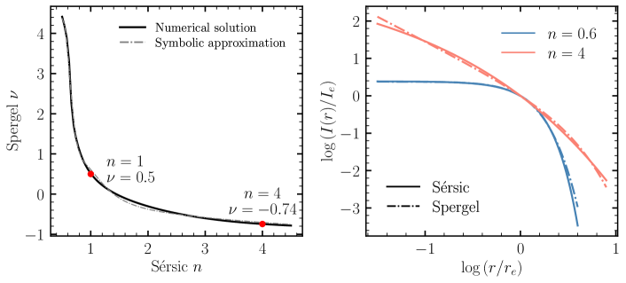
Figure 8: Correspondence between the Sérsic profile (C3) and the Spergel profile (C1). We fit a Spergel profile to each Sérsic while fixing the total luminosity and half-light radius. The black line in the left panel shows the best-fit Spergel index $\nu$ as a function of the Sérsic index $n$. We also provide a symbolic approximation to this relation in (C5), shown as the gray dashed-dotted line. In the right panel, two Sérsic profiles (solid) and their best-fit Spergel profiles (dashed-dotted) are shown. The Spergel profile approximates the Sérsic profile well at the small Sérsic index.

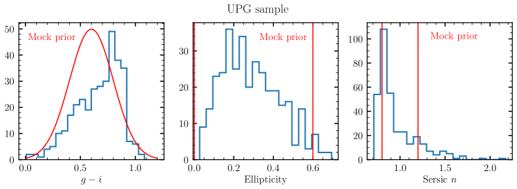
Figure 9: Distribution of UPGs (blue) and mock galaxies (red) in $g-i$ color, ellipticity, and Sérsic index $n$. We translate the Spergel index to the Sérsic index using Equation (C5). The mock galaxy population represents the real UDG/UPG population well.

In this appendix, we demonstrate that the Spergel profile can approximate the Sérsic profile and provide a lookup table for the correspondence between the Sérsic index $n$ and Spergel index $\nu$.

The surface brightness of a Spergel profile has the form (Spergel, 2010):

$$I_{\nu}(r)=\frac{c_{\nu}^{2}L_{0}}{2\pi r_{0}^{2}}f_{\nu}\left(\frac{c_{\nu}r}{r_{0}}\right),$$ (C1)

where

$$f_{\nu}(u)=\left(\frac{u}{2}\right)^{\nu}\frac{K_{\nu}(u)}{\Gamma(\nu+1)},$$ (C2)

and $K_{\nu}(u)$ is the Modified Bessel function of the second kind. The half-light radius is $r_{0}$, the total luminosity is $L_{0}$, and $c_{\nu}$ satisfies the equation $(1+\nu)f_{\nu+1}(c_{\nu})=1/4$. The Spergel profile has a simple analytical expression in Fourier space, making it easy to convolve with a PSF.

The surface brightness of a Sérsic profile follows (Sérsic, 1963; Graham & Driver, 2005):

$$I(r)=I_{\mathrm{e}}\exp\left\{-b_{n}\left[\left(\frac{r}{r_{\mathrm{e}}}\right)^{1/n}-1\right]\right\},$$ (C3)

where $r_{e}$ is the half-light radius, $I_{e}$ is the surface brightness at $r=r_{e}$, $n$ is the Sérsic index. The value of $b_{n}$ satisfies $\Gamma(2n)=2\gamma\left(2n,b_{n}\right)$, where $\gamma(a,x)$ is the incomplete gamma function. According to Graham & Driver (2005), the total luminosity of a Sérsic profile is given by

$$L_{0}=I_{e}r_{e}^{2}\,2\pi n\,e^{b_{n}}\left(b_{n}\right)^{-2n}\Gamma(2n).$$ (C4)

To study the correspondence between Sérsic and Spergel profiles, we generate Sérsic 1D profiles with different Sérsic indices using astropy, and try to fit the Sérsic profiles using the Spergel model. The Sérsic index ranges from $n=0.5$ to $n=4.5$, and both profiles are normalized at the half-light radius (see the right panel in Figure 8). For each Sérsic profile, we calculate the total luminosity $L_{0}$ according to (C4) and plug it into the Spergel profile (C1) as a fixed value. Therefore, only the Spergel index $\nu$ is allowed to vary during the fitting. The fitting uses the least squares fitting with Levenberg–Marquardt algorithm implemented in astropy.modeling.fitting, which is a commonly used robust algorithm to solve nonlinear least square fitting problems. The best-fit Spergel index $\nu$ as a function of the Sérsic index $n$ is shown in the left panel of Figure 8. A Spergel profile with $\nu=0.5$ is exactly an exponential profile with $n=1$. The de Vaucouleurs profile (de Vaucouleurs, 1948) with $n=4$ can be approximated by a Spergel profile with $\nu=-0.74$. As two examples, we show two Sérsic profiles (solid) and their best-fit Spergel profiles (dashed-dotted) in the right panel. Overall, the Spergel profile provides a good approximation for the Sérsic profile.

As shown in Figure 8, a Sérsic profile with a small Sérsic index ($0.5<n<1.5$) can be well-approximated by a Spergel profile, although the Spergel profile seems to be more extended than Sérsic in the outskirts. For a Sérsic profile with a high Sérsic index, the approximation gets worse at both small and large radii. Overall, the Spergel profile is a good approximation to Sérsic from $n\approx 0.5$ to $n\approx 4.5$. Using the symbolic regression package PySR (Cranmer, 2023), the best-fit relation between $n$ and $\nu$ for $0.5<n<4.5$ is given as follows:

$$\nu=1.06\,n^{-2.5}\cos(\sin(3.74/n))^{1/2}-0.365\,n^{1/2}$$ (C5)

It is well-known that the light profiles of low-mass galaxies are quite flat and can be described using Sérsic profiles with $0.5<n<1.5$ (e.g., van Dokkum et al., 2015; Lange et al., 2015; Greco et al., 2018; Zaritsky et al., 2021; Carlsten et al., 2021). It is thus reasonable to use Spergel profiles to model the LSBGs (§3.3) and enjoy its convenience in Fourier space.

Appendix D Completeness and Measurement Uncertainty

D.1 Completeness

The total completeness is a multiplication between the detection completeness and deblending completeness. Below we describe how we generate mock galaxies and derive the recovered fraction.

To estimate the detection completeness, we inject $\sim 700,000$ mock galaxies with single-Sérsic light profiles into the co-added images. The mock galaxies are generated using GalSim (Rowe et al., 2015) and are injected after being convolved with HSC PSF generated by hscPipe. We directly inject the mock galaxies into the co-added images without adding extra noise. The galaxies are placed randomly on the image but we require all mock galaxies to be separated by at least 80″ from each other to minimize the impact of mock galaxies on the image noise properties. We have also done extensive tests on injecting mock galaxies into the raw images, adding Poisson noise, and going through the entire data reduction pipeline using SynPipe (Huang et al., 2018b). This is very expensive in terms of both CPU time and disk space as we must run the full hscPipe. However, we find no noticeable difference in the completeness between this method and the direct injection to co-added images.

To resemble the real LSBG population in G18, we generate mock galaxies following uniform distributions in size ($2\arcsec\leqslant r_{e}\leqslant 21\arcsec$), surface brightness ($23\leqslant\overline{\mu}_{\rm eff}(g)\leqslant 28.5\ \mathrm{mag\ arcsec^{-2}}$), Sérsic index ($0.8<n<1.2$), and ellipticity ($0<\varepsilon<0.6$). They are randomly assigned to have a blue ($g-i=0.47,\ g-r=0.32$), medium ($g-i=0.64,\ g-r=0.43$), and red ($g-i=0.82,\ g-r=0.56$) color with equal chance. The ranges spanned by these colors and Sérsic indices cover most of the observed LSBGs in G18. Then we run the detection step described in §3.1 and cross-match the detection catalog with the input mock galaxy catalog to calculate completeness. We split the size and surface brightness range into 15 bins with $\Delta r_{e}=0\farcs 86$, $\Delta\overline{\mu}_{\mathrm{eff}}(g)=0.33\ \mathrm{mag\ arcsec}^{-2}$, and interpolate over bins using an isotropic Gaussian kernel with $\sigma=0.5$. We note that the size and surface brightness shown in Figure 3 are all the intrinsic values for the mock galaxies, which are different from the measured ones. We find negligible dependence of detection completeness on the Sérsic index, color, and ellipticity. Therefore, we neglect the dependence of detection completeness on parameters other than size and surface brightness hereafter.

For the deblending completeness, we inject 5000 mock Sérsic galaxies into the co-added images and run vanilla scarlet on them. The mock galaxies follow the same uniform distribution in size, surface brightness, ellipticity, Sérsic index as for deriving the detection completeness, but follow a Gaussian distribution in color: $g-i\sim\mathcal{N}(0.6,0.2^{2}),\ g-r=0.7\cdot(g-i)+\mathcal{N}(0,0.03^{2})$. We show the distribution of mock galaxies and UPGs in Figure 9. This mock galaxy population represents the real UDG/UPG population well. To be specific, the Gaussian color prior covers 86% of the UPGs within $1.5\sigma$, the ellipticity prior covers 98% of them, and the Sérsic index prior covers 60% of them. We measure the size and surface brightness on the scarlet models of the mock galaxies, then we apply the deblending cuts. We also find that the deblending cut mainly depends on the size and surface brightness.

D.2 Measurement Bias and Uncertainty

Due to the low-surface-brightness nature of LSBGs, their size, magnitude, surface brightness, and shape are hard to characterize and are typically associated with large uncertainties. Häussler et al. (2007) used mock single-Sérsic galaxies and parametric fitting codes to demonstrate that the estimated size and total magnitude are sensitive to local sky estimation and masking of neighboring objects. In the low-surface-brightness regime, the measured size and total magnitude can be quite biased and have large uncertainties. Therefore, measurement bias and uncertainty must be considered when studying the properties of LSBGs. Zaritsky et al. (2021, 2022) characterized their measurement bias and uncertainty by injecting mock Sérsic galaxies into co-added images and comparing the recovered properties with the truth. Tanoglidis et al. (2022) recently proposed a new method to estimate the measurement error using a Bayesian neural network. In this paper, we simply take the former method because of its simplicity.

In order to test how well we recover the photometric and structural parameters in our measurements (Sec 3.3), we take the 5000 mock Sérsic galaxies used for computing the deblending completeness and model them using the Spergel light profile. We model the bias and uncertainty in size, surface brightness, total magnitude, and color as a function of other parameters including size, surface brightness, and shape. However, we do not find any significant dependence of the bias on color, ellipticity, and the Spergel index. Thus we just model the bias and uncertainty as a function of the measured angular size $r_{e}$ and surface brightness $\overline{\mu}_{\mathrm{eff}}(g)$.

Given the size and surface brightness of our simulated galaxies, we set the range of the observed size and surface brightness to be $r_{e}\in[1\arcsec,15\arcsec],\ \overline{\mu}_{\mathrm{eff}}(g)\in[23,29]\,\mathrm{mag\ arcsec}^{-2}$. We then split the observed $r_{e}-\overline{\mu}_{\rm eff}(g)$ plane using an $8\times 8$ grid, and calculate the mean bias $\Delta X=X_{\rm truth}-X_{\rm meas}$ within each bin, where $X=\{\overline{\mu}_{\mathrm{eff}}(g),\ g-i,\ g-r\}$. For $r_{e}$, we calculate the relative bias $\Delta r_{e}/r_{e}$ instead because it is less dependent on the angular size. Then we interpolate over the grid using a multi-quadratic kernel with epsilon=0.5, smooth=1. Unlike Zaritsky et al. (2021) where they fit models in 4-D space, we find that interpolation works well enough in 2D and we do not use polynomial fitting to avoid meaningless results outside of the fitting range. We emphasize that the bias and uncertainty are modeled to be functions of the measured properties, not intrinsic ones, such that we can correct for bias based on our measurements.

For LSBGs in our sample, we apply corrections for the bias using the interpolated bias terms. We first correct for the bias in size, $g$-band average surface brightness, and $g-r$ and $g-i$ colors. Then we calculate the $g$-band total magnitude following $m_{g}=\overline{\mu}_{\rm eff}(g)-2.5\log(2\pi r_{e}^{2})$. The magnitudes and surface brightnesses in other bands are derived using $g$-band magnitude, surface brightness, and colors. In this way, we apply a self-consistent correction for the measurement biases to the data. The measurement uncertainty consists of a statistical uncertainty, which is determined by the shape of the likelihood (posterior) surface, and a systematic uncertainty, which is related to various factors including sky subtraction, neighbor contamination, etc. Unlike other parametric modeling codes such as imfit (Erwin, 2015) and the Tractor (Lang et al., 2016), scarlet does not explore the full posterior space but rather finds one optimal solution. Thus we have no access to the statistical error on the measured properties from scarlet. Fortunately, by comparing the recovered properties of mock galaxies with the truth, we can empirically estimate the measurement uncertainty without knowing the impact of each factor. Following the same method as that of calculating the bias, in each bin we compute the $1\sigma$ standard deviation of the difference between the truth and the bias-corrected measurement, then we interpolate over the grid. The measurement errors $\sigma(X)$ are shown in Figure 4 as contours, and they have the same units as the biases. We set minimum uncertainties to be $\sigma(r_{e})\geqslant 0.3,\ \sigma(\overline{\mu}_{\rm eff})\geqslant 0.05,\ \sigma(g-i)\geqslant 0.05$ to avoid meaningless uncertainty due to small statistics.

References

- Abbott et al. (2018) Abbott, T. M. C., Abdalla, F. B., Allam, S., et al. 2018, ApJS, 239, 18, doi: 10.3847/1538-4365/aae9f0
- Abraham et al. (2003) Abraham, R. G., van den Bergh, S., & Nair, P. 2003, ApJ, 588, 218, doi: 10.1086/373919
- Aihara et al. (2018) Aihara, H., Arimoto, N., Armstrong, R., et al. 2018, Publications of the Astronomical Society of Japan, 70, S4, doi: 10.1093/pasj/psx066
- Akhlaghi & Ichikawa (2015) Akhlaghi, M., & Ichikawa, T. 2015, ApJS, 220, 1, doi: 10.1088/0067-0049/220/1/1
- Amorisco & Loeb (2016) Amorisco, N. C., & Loeb, A. 2016, MNRAS, 459, L51, doi: 10.1093/mnrasl/slw055
- Astropy Collaboration et al. (2013) Astropy Collaboration, Robitaille, T. P., Tollerud, E. J., et al. 2013, A&A, 558, A33, doi: 10.1051/0004-6361/201322068
- Barbary (2016) Barbary, K. 2016, Journal of Open Source Software, 1(6), 58, doi: 10.21105/joss.0005
- Baxter et al. (2021) Baxter, D. C., Cooper, M. C., & Fillingham, S. P. 2021, MNRAS, 503, 1636, doi: 10.1093/mnras/stab523
- Behroozi et al. (2010) Behroozi, P. S., Conroy, C., & Wechsler, R. H. 2010, ApJ, 717, 379, doi: 10.1088/0004-637X/717/1/379
- Benavides et al. (2022) Benavides, J. A., Sales, L. V., Abadi, M. G., et al. 2022, arXiv e-prints, arXiv:2209.07539. https://arxiv.org/abs/2209.07539
- Benavides et al. (2021) —. 2021, Nature Astronomy, 5, 1255, doi: 10.1038/s41550-021-01458-1
- Bertin (2011) Bertin, E. 2011, in Astronomical Society of the Pacific Conference Series, Vol. 442, Astronomical Data Analysis Software and Systems XX, ed. I. N. Evans, A. Accomazzi, D. J. Mink, & A. H. Rots, 435
- Bertin & Arnouts (1996) Bertin, E., & Arnouts, S. 1996, A&AS, 117, 393, doi: 10.1051/aas:1996164
- Bland-Hawthorn & Gerhard (2016) Bland-Hawthorn, J., & Gerhard, O. 2016, ARA&A, 54, 529, doi: 10.1146/annurev-astro-081915-023441
- Blanton et al. (2011) Blanton, M. R., Kazin, E., Muna, D., Weaver, B. A., & Price-Whelan, A. 2011, AJ, 142, 31, doi: 10.1088/0004-6256/142/1/31
- Blanton et al. (2005) Blanton, M. R., Lupton, R. H., Schlegel, D. J., et al. 2005, ApJ, 631, 208, doi: 10.1086/431416
- Blanton & Roweis (2007) Blanton, M. R., & Roweis, S. 2007, AJ, 133, 734, doi: 10.1086/510127
- Bosch et al. (2018) Bosch, J., Armstrong, R., Bickerton, S., et al. 2018, PASJ, 70, S5, doi: 10.1093/pasj/psx080
- Bryan & Norman (1998) Bryan, G. L., & Norman, M. L. 1998, ApJ, 495, 80, doi: 10.1086/305262
- Caldwell & Bothun (1987) Caldwell, N., & Bothun, G. D. 1987, AJ, 94, 1126, doi: 10.1086/114550
- Cappellari (2013) Cappellari, M. 2013, ApJ, 778, L2, doi: 10.1088/2041-8205/778/1/L2
- Cardona-Barrero et al. (2020) Cardona-Barrero, S., Di Cintio, A., Brook, C. B. A., et al. 2020, MNRAS, 497, 4282, doi: 10.1093/mnras/staa2094
- Carlsten et al. (2022a) Carlsten, S. G., Greene, J. E., Beaton, R. L., Danieli, S., & Greco, J. P. 2022a, ApJ, 933, 47, doi: 10.3847/1538-4357/ac6fd7
- Carlsten et al. (2022b) Carlsten, S. G., Greene, J. E., Beaton, R. L., & Greco, J. P. 2022b, ApJ, 927, 44, doi: 10.3847/1538-4357/ac457e
- Carlsten et al. (2021) Carlsten, S. G., Greene, J. E., Greco, J. P., Beaton, R. L., & Kado-Fong, E. 2021, ApJ, 922, 267, doi: 10.3847/1538-4357/ac2581
- Chabrier (2003) Chabrier, G. 2003, PASP, 115, 763, doi: 10.1086/376392
- Chamba et al. (2022) Chamba, N., Trujillo, I., & Knapen, J. H. 2022, arXiv e-prints, arXiv:2209.05497. https://arxiv.org/abs/2209.05497
- Chan et al. (2018) Chan, T. K., Kereš, D., Wetzel, A., et al. 2018, MNRAS, 478, 906, doi: 10.1093/mnras/sty1153
- Cohen et al. (2018) Cohen, Y., van Dokkum, P., Danieli, S., et al. 2018, ApJ, 868, 96, doi: 10.3847/1538-4357/aae7c8
- Conselice (2003) Conselice, C. J. 2003, ApJS, 147, 1, doi: 10.1086/375001
- Cranmer (2023) Cranmer, M. 2023, arXiv e-prints, arXiv:2305.01582, doi: 10.48550/arXiv.2305.01582
- Dalcanton et al. (1997a) Dalcanton, J. J., Spergel, D. N., Gunn, J. E., Schmidt, M., & Schneider, D. P. 1997a, AJ, 114, 635, doi: 10.1086/118499
- Dalcanton et al. (1997b) —. 1997b, AJ, 114, 635, doi: 10.1086/118499
- Danieli & van Dokkum (2019) Danieli, S., & van Dokkum, P. 2019, ApJ, 875, 155, doi: 10.3847/1538-4357/ab14f3
- Danieli et al. (2019) Danieli, S., van Dokkum, P., Conroy, C., Abraham, R., & Romanowsky, A. J. 2019, ApJ, 874, L12, doi: 10.3847/2041-8213/ab0e8c
- Danieli et al. (2020) Danieli, S., Lokhorst, D., Zhang, J., et al. 2020, ApJ, 894, 119, doi: 10.3847/1538-4357/ab88a8
- Danieli et al. (2022) Danieli, S., van Dokkum, P., Trujillo-Gomez, S., et al. 2022, ApJ, 927, L28, doi: 10.3847/2041-8213/ac590a
- de Vaucouleurs (1948) de Vaucouleurs, G. 1948, Annales d’Astrophysique, 11, 247
- Dey et al. (2019) Dey, A., Schlegel, D. J., Lang, D., et al. 2019, AJ, 157, 168, doi: 10.3847/1538-3881/ab089d
- Di Cintio et al. (2017) Di Cintio, A., Brook, C. B., Dutton, A. A., et al. 2017, MNRAS, 466, L1, doi: 10.1093/mnrasl/slw210
- Diemer (2018) Diemer, B. 2018, ApJS, 239, 35, doi: 10.3847/1538-4365/aaee8c
- Du et al. (2020) Du, W., Cheng, C., Zheng, Z., & Wu, H. 2020, AJ, 159, 138, doi: 10.3847/1538-3881/ab6efb
- Eigenthaler et al. (2018) Eigenthaler, P., Puzia, T. H., Taylor, M. A., et al. 2018, ApJ, 855, 142, doi: 10.3847/1538-4357/aaab60
- Erwin (2015) Erwin, P. 2015, ApJ, 799, 226, doi: 10.1088/0004-637X/799/2/226
- Ferrarese et al. (2020) Ferrarese, L., Côté, P., MacArthur, L. A., et al. 2020, ApJ, 890, 128, doi: 10.3847/1538-4357/ab339f
- Ferré-Mateu et al. (2018) Ferré-Mateu, A., Alabi, A., Forbes, D. A., et al. 2018, MNRAS, 479, 4891, doi: 10.1093/mnras/sty1597
- Fliri & Trujillo (2016) Fliri, J., & Trujillo, I. 2016, MNRAS, 456, 1359, doi: 10.1093/mnras/stv2686
- Font et al. (2022) Font, A. S., McCarthy, I. G., Belokurov, V., Brown, S. T., & Stafford, S. G. 2022, MNRAS, 511, 1544, doi: 10.1093/mnras/stac183
- Forbes et al. (2020) Forbes, D. A., Alabi, A., Romanowsky, A. J., Brodie, J. P., & Arimoto, N. 2020, MNRAS, 492, 4874, doi: 10.1093/mnras/staa180
- Gaia Collaboration et al. (2016) Gaia Collaboration, Prusti, T., de Bruijne, J. H. J., et al. 2016, A&A, 595, A1, doi: 10.1051/0004-6361/201629272
- Gaia Collaboration et al. (2018) Gaia Collaboration, Brown, A. G. A., Vallenari, A., et al. 2018, A&A, 616, A1, doi: 10.1051/0004-6361/201833051
- Gannon et al. (2022) Gannon, J. S., Forbes, D. A., Romanowsky, A. J., et al. 2022, MNRAS, 510, 946, doi: 10.1093/mnras/stab3297
- Geha et al. (2017) Geha, M., Wechsler, R. H., Mao, Y.-Y., et al. 2017, ApJ, 847, 4, doi: 10.3847/1538-4357/aa8626
- Graham & Driver (2005) Graham, A. W., & Driver, S. P. 2005, PASA, 22, 118, doi: 10.1071/AS05001
- Graham & Guzmán (2003) Graham, A. W., & Guzmán, R. 2003, AJ, 125, 2936, doi: 10.1086/374992
- Greco et al. (2018) Greco, J. P., Greene, J. E., Strauss, M. A., et al. 2018, ApJ, 857, 104, doi: 10.3847/1538-4357/aab842
- Greene et al. (2022) Greene, J. E., Greco, J. P., Goulding, A. D., et al. 2022, arXiv e-prints, arXiv:2204.11883. https://arxiv.org/abs/2204.11883
- Gu et al. (2018) Gu, M., Conroy, C., Law, D., et al. 2018, ApJ, 859, 37, doi: 10.3847/1538-4357/aabbae
- Harris et al. (2020) Harris, C. R., Millman, K. J., van der Walt, S. J., et al. 2020, Nature, 585, 357, doi: 10.1038/s41586-020-2649-2
- Häussler et al. (2007) Häussler, B., McIntosh, D. H., Barden, M., et al. 2007, ApJS, 172, 615, doi: 10.1086/518836
- Hearin et al. (2017) Hearin, A. P., Campbell, D., Tollerud, E., et al. 2017, AJ, 154, 190, doi: 10.3847/1538-3881/aa859f
- Herrmann et al. (2016) Herrmann, K. A., Hunter, D. A., Zhang, H.-X., & Elmegreen, B. G. 2016, AJ, 152, 177, doi: 10.3847/0004-6256/152/6/177
- Huang et al. (2018a) Huang, S., Leauthaud, A., Greene, J. E., et al. 2018a, MNRAS, 475, 3348, doi: 10.1093/mnras/stx3200
- Huang et al. (2018b) Huang, S., Leauthaud, A., Murata, R., et al. 2018b, PASJ, 70, S6, doi: 10.1093/pasj/psx126
- Hunter (2007) Hunter, J. D. 2007, Computing in Science Engineering, 9, 90, doi: 10.1109/MCSE.2007.55
- Impey et al. (1988) Impey, C., Bothun, G., & Malin, D. 1988, ApJ, 330, 634, doi: 10.1086/166500
- Into & Portinari (2013) Into, T., & Portinari, L. 2013, MNRAS, 430, 2715, doi: 10.1093/mnras/stt071
- Irwin (1985) Irwin, M. J. 1985, MNRAS, 214, 575, doi: 10.1093/mnras/214.4.575
- Ivezić et al. (2019) Ivezić, Ž., Kahn, S. M., Tyson, J. A., et al. 2019, ApJ, 873, 111, doi: 10.3847/1538-4357/ab042c
- Janssens et al. (2017) Janssens, S., Abraham, R., Brodie, J., et al. 2017, ApJ, 839, L17, doi: 10.3847/2041-8213/aa667d
- Jiang et al. (2019) Jiang, F., Dekel, A., Freundlich, J., et al. 2019, MNRAS, 487, 5272, doi: 10.1093/mnras/stz1499
- Jones et al. (2001) Jones, E., Oliphant, T., Peterson, P., et al. 2001, SciPy: Open source scientific tools for Python. http://www.scipy.org/
- Jurić et al. (2017) Jurić, M., Kantor, J., Lim, K. T., et al. 2017, in Astronomical Society of the Pacific Conference Series, Vol. 512, Astronomical Data Analysis Software and Systems XXV, ed. N. P. F. Lorente, K. Shortridge, & R. Wayth, 279. https://arxiv.org/abs/1512.07914
- Kado-Fong et al. (2022) Kado-Fong, E., Greene, J. E., Huang, S., & Goulding, A. 2022, ApJ, 941, 11, doi: 10.3847/1538-4357/ac9964
- Kado-Fong et al. (2018) Kado-Fong, E., Greene, J. E., Hendel, D., et al. 2018, ApJ, 866, 103, doi: 10.3847/1538-4357/aae0f0
- Kado-Fong et al. (2021) Kado-Fong, E., Petrescu, M., Mohammad, M., et al. 2021, ApJ, 920, 72, doi: 10.3847/1538-4357/ac15f0
- Kadowaki et al. (2021) Kadowaki, J., Zaritsky, D., Donnerstein, R. L., et al. 2021, ApJ, 923, 257, doi: 10.3847/1538-4357/ac2948
- Karachentsev et al. (2013) Karachentsev, I. D., Makarov, D. I., & Kaisina, E. I. 2013, AJ, 145, 101, doi: 10.1088/0004-6256/145/4/101
- Karunakaran & Zaritsky (2022) Karunakaran, A., & Zaritsky, D. 2022, arXiv e-prints, arXiv:2210.00009. https://arxiv.org/abs/2210.00009
- Keim et al. (2022) Keim, M. A., Dokkum, P. v., Danieli, S., et al. 2022, ApJ, 935, 160, doi: 10.3847/1538-4357/ac7dab
- Koda et al. (2015) Koda, J., Yagi, M., Yamanoi, H., & Komiyama, Y. 2015, ApJ, 807, L2, doi: 10.1088/2041-8205/807/1/L2
- Kong et al. (2022) Kong, D., Kaplinghat, M., Yu, H.-B., Fraternali, F., & Mancera Piña, P. E. 2022, ApJ, 936, 166, doi: 10.3847/1538-4357/ac8875
- La Marca et al. (2022) La Marca, A., Iodice, E., Cantiello, M., et al. 2022, A&A, 665, A105, doi: 10.1051/0004-6361/202142367
- Lang et al. (2016) Lang, D., Hogg, D. W., & Mykytyn, D. 2016, The Tractor: Probabilistic astronomical source detection and measurement, Astrophysics Source Code Library, record ascl:1604.008. http://ascl.net/1604.008
- Lange et al. (2015) Lange, R., Driver, S. P., Robotham, A. S. G., et al. 2015, MNRAS, 447, 2603, doi: 10.1093/mnras/stu2467
- Lee et al. (2017) Lee, M. G., Kang, J., Lee, J. H., & Jang, I. S. 2017, ApJ, 844, 157, doi: 10.3847/1538-4357/aa78fb
- Leisman et al. (2017) Leisman, L., Haynes, M. P., Janowiecki, S., et al. 2017, ApJ, 842, 133, doi: 10.3847/1538-4357/aa7575
- Li et al. (2023) Li, J., Greene, J. E., Greco, J., et al. 2023, arXiv e-prints, arXiv:2302.14108, doi: 10.48550/arXiv.2302.14108
- Li et al. (2022) Li, J., Huang, S., Leauthaud, A., et al. 2022, MNRAS, 515, 5335, doi: 10.1093/mnras/stac2121
- Liao et al. (2019) Liao, S., Gao, L., Frenk, C. S., et al. 2019, MNRAS, 490, 5182, doi: 10.1093/mnras/stz2969
- Licquia & Newman (2015) Licquia, T. C., & Newman, J. A. 2015, ApJ, 806, 96, doi: 10.1088/0004-637X/806/1/96
- Lim et al. (2020) Lim, S., Côté, P., Peng, E. W., et al. 2020, ApJ, 899, 69, doi: 10.3847/1538-4357/aba433
- Liu et al. (2022) Liu, Q., Abraham, R., Gilhuly, C., et al. 2022, ApJ, 925, 219, doi: 10.3847/1538-4357/ac32c6
- Lotz et al. (2004) Lotz, J. M., Primack, J., & Madau, P. 2004, AJ, 128, 163, doi: 10.1086/421849
- Lotz et al. (2008) Lotz, J. M., Davis, M., Faber, S. M., et al. 2008, ApJ, 672, 177, doi: 10.1086/523659
- LSST Science Collaboration et al. (2009) LSST Science Collaboration, Abell, P. A., Allison, J., et al. 2009, arXiv e-prints, arXiv:0912.0201. https://arxiv.org/abs/0912.0201
- Mancera Piña et al. (2019a) Mancera Piña, P. E., Aguerri, J. A. L., Peletier, R. F., et al. 2019a, MNRAS, 485, 1036, doi: 10.1093/mnras/stz238
- Mancera Piña et al. (2022a) Mancera Piña, P. E., Fraternali, F., Oosterloo, T., et al. 2022a, MNRAS, 514, 3329, doi: 10.1093/mnras/stac1508
- Mancera Piña et al. (2022b) —. 2022b, MNRAS, 512, 3230, doi: 10.1093/mnras/stab3491
- Mancera Piña et al. (2018) Mancera Piña, P. E., Peletier, R. F., Aguerri, J. A. L., et al. 2018, MNRAS, 481, 4381, doi: 10.1093/mnras/sty2574
- Mancera Piña et al. (2019b) Mancera Piña, P. E., Fraternali, F., Adams, E. A. K., et al. 2019b, ApJ, 883, L33, doi: 10.3847/2041-8213/ab40c7
- Mancera Piña et al. (2020) Mancera Piña, P. E., Fraternali, F., Oman, K. A., et al. 2020, MNRAS, 495, 3636, doi: 10.1093/mnras/staa1256
- Mao et al. (2021) Mao, Y.-Y., Geha, M., Wechsler, R. H., et al. 2021, ApJ, 907, 85, doi: 10.3847/1538-4357/abce58
- Martin et al. (2019) Martin, G., Kaviraj, S., Laigle, C., et al. 2019, MNRAS, 485, 796, doi: 10.1093/mnras/stz356
- McConnachie (2012) McConnachie, A. W. 2012, AJ, 144, 4, doi: 10.1088/0004-6256/144/1/4
- McGaugh et al. (1995) McGaugh, S. S., Bothun, G. D., & Schombert, J. M. 1995, AJ, 110, 573, doi: 10.1086/117543
- Melchior et al. (2019) Melchior, P., Joseph, R., & Moolekamp, F. 2019, arXiv e-prints, arXiv:1910.10094. https://arxiv.org/abs/1910.10094
- Melchior et al. (2021) Melchior, P., Joseph, R., Sanchez, J., MacCrann, N., & Gruen, D. 2021, Nature Reviews Physics, 3, 712, doi: 10.1038/s42254-021-00353-y
- Melchior et al. (2018) Melchior, P., Moolekamp, F., Jerdee, M., et al. 2018, Astronomy and Computing, 24, 129, doi: 10.1016/j.ascom.2018.07.001
- Mihos et al. (2015) Mihos, J. C., Durrell, P. R., Ferrarese, L., et al. 2015, ApJ, 809, L21, doi: 10.1088/2041-8205/809/2/L21
- Miller et al. (2019) Miller, T. B., van Dokkum, P., Mowla, L., & van der Wel, A. 2019, ApJ, 872, L14, doi: 10.3847/2041-8213/ab0380
- Misgeld & Hilker (2011) Misgeld, I., & Hilker, M. 2011, MNRAS, 414, 3699, doi: 10.1111/j.1365-2966.2011.18669.x
- Misgeld et al. (2008) Misgeld, I., Mieske, S., & Hilker, M. 2008, A&A, 486, 697, doi: 10.1051/0004-6361:200810014
- Miyazaki et al. (2012) Miyazaki, S., Komiyama, Y., Nakaya, H., et al. 2012, Proc.SPIE, 8446, 8446 , doi: 10.1117/12.926844
- Miyazaki et al. (2018) Miyazaki, S., Komiyama, Y., Kawanomoto, S., et al. 2018, PASJ, 70, S1, doi: 10.1093/pasj/psx063
- Moster et al. (2013) Moster, B. P., Naab, T., & White, S. D. M. 2013, MNRAS, 428, 3121, doi: 10.1093/mnras/sts261
- Mowla et al. (2019) Mowla, L., van der Wel, A., van Dokkum, P., & Miller, T. B. 2019, ApJ, 872, L13, doi: 10.3847/2041-8213/ab0379
- Mowla et al. (2017) Mowla, L., van Dokkum, P., Merritt, A., et al. 2017, ApJ, 851, 27, doi: 10.3847/1538-4357/aa961b
- Muñoz et al. (2015) Muñoz, R. P., Eigenthaler, P., Puzia, T. H., et al. 2015, ApJ, 813, L15, doi: 10.1088/2041-8205/813/1/L15
- Nashimoto et al. (2022) Nashimoto, M., Tanaka, M., Chiba, M., et al. 2022, arXiv e-prints, arXiv:2207.11992. https://arxiv.org/abs/2207.11992
- Neumayer et al. (2020) Neumayer, N., Seth, A., & Böker, T. 2020, A&A Rev., 28, 4, doi: 10.1007/s00159-020-00125-0
- Oke & Gunn (1983) Oke, J. B., & Gunn, J. E. 1983, ApJ, 266, 713, doi: 10.1086/160817
- Pandya et al. (2018) Pandya, V., Romanowsky, A. J., Laine, S., et al. 2018, ApJ, 858, 29, doi: 10.3847/1538-4357/aab498
- Planck Collaboration et al. (2016) Planck Collaboration, Ade, P. A. R., Aghanim, N., et al. 2016, A&A, 594, A13, doi: 10.1051/0004-6361/201525830
- Posti et al. (2019) Posti, L., Fraternali, F., & Marasco, A. 2019, A&A, 626, A56, doi: 10.1051/0004-6361/201935553
- Prole et al. (2019) Prole, D. J., van der Burg, R. F. J., Hilker, M., & Davies, J. I. 2019, MNRAS, 488, 2143, doi: 10.1093/mnras/stz1843
- Rodriguez-Gomez et al. (2019) Rodriguez-Gomez, V., Snyder, G. F., Lotz, J. M., et al. 2019, MNRAS, 483, 4140, doi: 10.1093/mnras/sty3345
- Román et al. (2019) Román, J., Beasley, M. A., Ruiz-Lara, T., & Valls-Gabaud, D. 2019, MNRAS, 486, 823, doi: 10.1093/mnras/stz835
- Román et al. (2021) Román, J., Castilla, A., & Pascual-Granado, J. 2021, A&A, 656, A44, doi: 10.1051/0004-6361/202142161
- Román & Trujillo (2017a) Román, J., & Trujillo, I. 2017a, MNRAS, 468, 4039, doi: 10.1093/mnras/stx694
- Román & Trujillo (2017b) —. 2017b, MNRAS, 468, 703, doi: 10.1093/mnras/stx438
- Rowe et al. (2015) Rowe, B. T. P., Jarvis, M., Mandelbaum, R., et al. 2015, Astronomy and Computing, 10, 121, doi: 10.1016/j.ascom.2015.02.002
- Sandage & Binggeli (1984) Sandage, A., & Binggeli, B. 1984, AJ, 89, 919, doi: 10.1086/113588
- Schlafly & Finkbeiner (2011) Schlafly, E. F., & Finkbeiner, D. P. 2011, ApJ, 737, 103, doi: 10.1088/0004-637X/737/2/103
- Schlegel et al. (1998) Schlegel, D. J., Finkbeiner, D. P., & Davis, M. 1998, ApJ, 500, 525, doi: 10.1086/305772
- Sérsic (1963) Sérsic, J. L. 1963, Boletin de la Asociacion Argentina de Astronomia La Plata Argentina, 6, 41
- Simon (2019) Simon, J. D. 2019, ARA&A, 57, 375, doi: 10.1146/annurev-astro-091918-104453
- Smith Castelli et al. (2008) Smith Castelli, A. V., Bassino, L. P., Richtler, T., et al. 2008, MNRAS, 386, 2311, doi: 10.1111/j.1365-2966.2008.13211.x
- Somalwar et al. (2020) Somalwar, J. J., Greene, J. E., Greco, J. P., et al. 2020, ApJ, 902, 45, doi: 10.3847/1538-4357/abb1b2
- Spergel (2010) Spergel, D. N. 2010, ApJS, 191, 58, doi: 10.1088/0067-0049/191/1/58
- Starck et al. (2015) Starck, J.-L., Murtagh, F., & Bertero, M. 2015, Starlet Transform in Astronomical Data Processing, ed. O. Scherzer (New York, NY: Springer New York), 2053–2098, doi: 10.1007/978-1-4939-0790-8_34
- Tanoglidis et al. (2022) Tanoglidis, D., Ćiprijanović, A., & Drlica-Wagner, A. 2022, arXiv e-prints, arXiv:2207.03471. https://arxiv.org/abs/2207.03471
- Tanoglidis et al. (2021) Tanoglidis, D., Drlica-Wagner, A., Wei, K., et al. 2021, ApJS, 252, 18, doi: 10.3847/1538-4365/abca89
- Tremmel et al. (2020) Tremmel, M., Wright, A. C., Brooks, A. M., et al. 2020, MNRAS, 497, 2786, doi: 10.1093/mnras/staa2015
- Trujillo et al. (2020) Trujillo, I., Chamba, N., & Knapen, J. H. 2020, MNRAS, 493, 87, doi: 10.1093/mnras/staa236
- Trujillo et al. (2007) Trujillo, I., Conselice, C. J., Bundy, K., et al. 2007, MNRAS, 382, 109, doi: 10.1111/j.1365-2966.2007.12388.x
- Trujillo et al. (2017) Trujillo, I., Roman, J., Filho, M., & Sánchez Almeida, J. 2017, ApJ, 836, 191, doi: 10.3847/1538-4357/aa5cbb
- van der Burg et al. (2016) van der Burg, R. F. J., Muzzin, A., & Hoekstra, H. 2016, A&A, 590, A20, doi: 10.1051/0004-6361/201628222
- van der Burg et al. (2017) van der Burg, R. F. J., Hoekstra, H., Muzzin, A., et al. 2017, A&A, 607, A79, doi: 10.1051/0004-6361/201731335
- van Dokkum et al. (2019) van Dokkum, P., Danieli, S., Abraham, R., Conroy, C., & Romanowsky, A. J. 2019, ApJ, 874, L5, doi: 10.3847/2041-8213/ab0d92
- van Dokkum et al. (2017) van Dokkum, P., Abraham, R., Romanowsky, A. J., et al. 2017, ApJ, 844, L11, doi: 10.3847/2041-8213/aa7ca2
- van Dokkum et al. (2018) van Dokkum, P., Danieli, S., Cohen, Y., et al. 2018, Nature, 555, 629, doi: 10.1038/nature25767
- van Dokkum et al. (2022a) van Dokkum, P., Shen, Z., Romanowsky, A. J., et al. 2022a, arXiv e-prints, arXiv:2207.07129. https://arxiv.org/abs/2207.07129
- van Dokkum et al. (2022b) van Dokkum, P., Shen, Z., Keim, M. A., et al. 2022b, Nature, 605, 435, doi: 10.1038/s41586-022-04665-6
- van Dokkum et al. (2015) van Dokkum, P. G., Abraham, R., Merritt, A., et al. 2015, ApJ, 798, L45, doi: 10.1088/2041-8205/798/2/L45
- van Dokkum et al. (2013) van Dokkum, P. G., Leja, J., Nelson, E. J., et al. 2013, ApJ, 771, L35, doi: 10.1088/2041-8205/771/2/L35
- Van Nest et al. (2022) Van Nest, J. D., Munshi, F., Wright, A. C., et al. 2022, ApJ, 926, 92, doi: 10.3847/1538-4357/ac43b7
- Venhola et al. (2022) Venhola, A., Peletier, R. F., Salo, H., et al. 2022, A&A, 662, A43, doi: 10.1051/0004-6361/202141756
- Villaume et al. (2022) Villaume, A., Romanowsky, A. J., Brodie, J., et al. 2022, ApJ, 924, 32, doi: 10.3847/1538-4357/ac341e
- Wang et al. (2021) Wang, W., Takada, M., Li, X., et al. 2021, MNRAS, 500, 3776, doi: 10.1093/mnras/staa3495
- Wasserman et al. (2019) Wasserman, A., van Dokkum, P., Romanowsky, A. J., et al. 2019, ApJ, 885, 155, doi: 10.3847/1538-4357/ab3eb9
- Willmer (2018) Willmer, C. N. A. 2018, ApJS, 236, 47, doi: 10.3847/1538-4365/aabfdf
- Wright et al. (2021) Wright, A. C., Tremmel, M., Brooks, A. M., et al. 2021, MNRAS, 502, 5370, doi: 10.1093/mnras/stab081
- Wu et al. (2022) Wu, J. F., Peek, J. E. G., Tollerud, E. J., et al. 2022, ApJ, 927, 121, doi: 10.3847/1538-4357/ac4eea
- Yagi et al. (2016) Yagi, M., Koda, J., Komiyama, Y., & Yamanoi, H. 2016, ApJS, 225, 11, doi: 10.3847/0067-0049/225/1/11
- York et al. (2000) York, D. G., Adelman, J., Anderson, John E., J., et al. 2000, AJ, 120, 1579, doi: 10.1086/301513
- Zaritsky et al. (2021) Zaritsky, D., Donnerstein, R., Karunakaran, A., et al. 2021, ApJS, 257, 60, doi: 10.3847/1538-4365/ac2607
- Zaritsky et al. (2022) —. 2022, ApJS, 261, 11, doi: 10.3847/1538-4365/ac6ceb
- Zaritsky et al. (2019) Zaritsky, D., Donnerstein, R., Dey, A., et al. 2019, ApJS, 240, 1, doi: 10.3847/1538-4365/aaefe9