Fast and Efficient Scene Categorization
for Autonomous Driving using VAEs

Abstract

Scene categorization is a useful precursor task that provides prior knowledge for many advanced computer vision tasks with a broad range of applications in content-based image indexing and retrieval systems. Despite the success of data driven approaches in the field of computer vision such as object detection, semantic segmentation, etc., their application in learning high-level features for scene recognition has not achieved the same level of success. We propose to generate a fast and efficient intermediate interpretable generalized global descriptor that captures coarse features from the image and use a classification head to map the descriptors to 3 scene categories: Rural, Urban and Suburban. We train a Variational Autoencoder in an unsupervised manner and map images to a constrained multi-dimensional latent space and use the latent vectors as compact embeddings that serve as global descriptors for images. The experimental results evidence that the VAE latent vectors capture coarse information from the image, supporting their usage as global descriptors. The proposed global descriptor is very compact with an embedding length of 128, significantly faster to compute, and is robust to seasonal and illuminational changes, while capturing sufficient scene information required for scene categorization.

Keywords: Scene Categorization, Image Embeddings, Coarse Features, Variational Autoencoders

1 Introduction

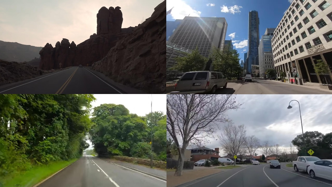
Figure 1: Images from the Scene Categorization Dataset. Top Left: Rural (Utah), Top Right: Urban (Toronto), Bottom Left: Rural (Stockport to Buxton), Bottom Right: Suburban (Melbourne)

.

Scene categorization is a precursor task with a broad range of applications in content-based image indexing and retrieval systems. Content Based Image Retrieval (CBIR) uses the visual content of a given query image to find the closest match in a large image database [Aliajni and Rahtu, 2020]. The retrieval accuracy of CBIR depends on both the feature representation and the similarity metric. The retrieval process can be accelerated by selectively searching based on certain scene categories e.g. given a query image with multiple high-rise buildings, searching the rural regions would not be beneficial and can be skipped. The knowledge about the scene category can also assist in context-aware object detection, action recognition, and scene understanding and provides prior knowledge for other advanced computer vision tasks [Khan et al., 2016, Xiao et al., 2010].

In autonomous driving scenarios, location context provides an important prior for parameterising autonomous behaviour. Generally GPS data is used to determine if the vehicle has entered the city limits, where additional caution is required e.g. to set the pedestrian detection threshold to watch out for pedestrians in populated regions. However, such an approach requires apriori labelling of the environment and due to rapid development of regions around the cities and suburbs, it has become increasingly hard to distinguish such regions of interest only using GPS coordinates. A more scalable and lower cost approach would be to automatically determine the scene type at the edge using locally sensed data.

We present a deep learning based unsupervised holistic approach that directly encodes coarse information in the multi-dimensional latent space without explicitly recognizing objects, their semantics or capturing fine details. Models equipped with intermediate representations train faster, achieve higher task performance, and generalize better to previously unseen environments [Zhou et al., 2019]. To this end, rather than directly mapping the input image to the required scene categories as with classic data-driven classification solutions, we propose to generate an intermediate generalized global descriptor that captures coarse features from the image and use a separate classification head to map the descriptors to scene categories. More specifically, we use an unsupervised convolutional Variational Autoencoder (VAE) to map images to a multi-dimensional latent space. We propose to use the latent vectors directly as global descriptors, which are then mapped to 3 scene categories: Rural, Urban and Suburban, using a supervised classification head that takes in these descriptors as input.

2 Background

The success of deep learning in the field of computer vision over the past decade has resulted in dramatic improvements in performance in areas such as object recognition, detection, segmentation, etc. However, the performance of scene recognition is still not sufficient to some extent because of complex configurations [Xie et al., 2020]. Early work on scene categorization includes [Oliva and Torralba, 2001] where the authors proposed a computational model of the recognition of real world scenes that bypasses the segmentation and the processing of individual objects or regions. Notable early global image descriptor approaches include aggregation of local keypoint descriptors through Bag of Words (BoW) [Csurka et al., 2004], Fisher Vectors (FV) [Perronnin et al., 2010, Sanchez et al., 2013] and Vector of Locally Aggregated Descriptors (VLAD) [Jégou et al., 2010]. More recently, researchers have also used Histogram of Oriented Gradients (HOG) and its extensions such as Pyramid HOG (PHOG) for mapping and localization [Garcia-Fidalgo and Ortiz, 2017]. Although these approaches have shown strong performance in constrained settings, they lack the repeatability and robustness required to deal with the challenging variability that occurs in natural scenes caused due to different times of the day, weather, lighting and seasons [Ramachandran and McDonald, 2019].

To overcome these issues recent research has focussed on the use of learned global descriptors. Probably the most notable here is NetVLAD which reformulated VLAD through the use of a deep learning architecture [Arandjelovic et al., 2016] resulting in a CNN based feature extractor using weak supervision to learn a distance metric based on the triplet loss.

Variatonal Autoencoder (VAE), introduced by [Kingma and Welling, 2013], maps images to a multi-dimensional standard normal latent space. Although since the introduction of the CelebA dataset [Liu et al., 2015] multiple implementations of VAEs have shown success in generating human faces, VAEs often produce blurry and less saturated reconstructions and have been shown to lack the ability to generalize and generate high-resolution images for domains that exhibit multiple complex variations e.g. realistic natural landscape images. Besides their use as generative models, VAEs have also been used to infer one or more scalar variables from images in the context of Autonomous Driving such as for vehicle control [Amini et al., 2018].

A number of researchers have developed datasets to accelerate progress in general scene recognition. Examples include MIT Indoor67 [Quattoni and Torralba, 2009], SUN [Xiao et al., 2010], and Places 365 [Zhou et al., 2017]. Whilst these datasets capture a very wide variety of scenes they lack suitability when developing scene categorisation techniques that are specific to autonomous driving. Given this, in our research we choose to use images from public driving datasets such as Oxford Robotcar [Maddern et al., 2017] in an unsupervised manner and curate our own evaluation dataset targeted at our domain of interest.

In this paper, we propose to use a trained Variational Autoencoder to map images to a multi-dimensional latent space and use the latent vectors as compact embeddings that serve directly as global descriptors for images. To the best of our knowledge, this is the first time VAE latent vectors are used as global image descriptors. In detail, we train a convolutional Variational Autoencoder in an unsupervised manner with images from Oxford Robotcar dataset [Maddern et al., 2017] that exhibit strong visual changes caused by seasons, weather, time of the day, etc. and use the latent vectors inferred using the encoder as global descriptors. We show that VAE encoder captures coarse features of the image and produces a mapping in multi-dimensional standard normal latent space. We then use a simple two-layer linear classification perceptron head to map the global descriptors to required scene categories: Rural, Urban and Suburban.

3 Methodology

In our method, we train a Variational Autoencoder from scratch on images from publicly available Oxford Robotcar dataset [Maddern et al., 2017] in an unsupervised manner. We then obtain latent vectors during inference and use them as compact embeddings that serve as global descriptors. The global descriptors are then used as input to a simple linear classifier that maps them to 3 scene categories: Rural, Urban and Suburban. Figure 2 provides a high-level view of our overall architecture.

Figure 2: Overall system architecture for scene categorization. Input and output for each module is shown in the bottom row including an example.

3.1 Scene Embedding

In order to evaluate the performance of different VAEs for scene embedding, we train multiple variants on 3 Oxford Robotcar traversals 2014-12-09-13-21-02 (Winter Day), 2014-12-10-18-10-50 (Winter Night), and 2015-05-19-14-06-38 (Summer Day). These traversals exhibit changes due to seasons and time of the day. We sub-sample each traversal using the sequential adaptive sampling strategy reported in [Ramachandran and McDonald, 2021] with parameters $\tau_{d_{\text{acc}}}=5m$ and $\tau_{\theta_{\text{acc}}}=15^{\circ}$ to obtain 1787, 1879 and 1825 visually dissimilar images respectively. The following variants of VAE are trained:

• BetaVAE [Higgins et al., 2016]

• CategoricalVAE [Jang et al., 2016]

• DFCVAE [Hou et al., 2017]

• DIPVAE [Kumar et al., 2017]

• InfoVAE [Zhao et al., 2017]

• LogCoshVAE [Chen et al., 2019]

• MIWAE [Rainforth et al., 2018]

• VAE (Vanilla) [Kingma and Welling, 2013]

(a) 48 random input images from Oxford Robotcar dataset

(b) VAE (499 Epochs) [Kingma and Welling, 2013]

(c) BetaVAE (103 Epochs) [Higgins et al., 2016]

(d) CategoricalVAE (114 Epochs) [Jang et al., 2016]

(e) DFCVAE (107 Epochs) [Hou et al., 2017]

(f) DIPVAE (178 Epochs) [Kumar et al., 2017]

(g) InfoVAE (119 Epochs) [Zhao et al., 2017]

(h) LogCoshVAE (104 Epochs) [Chen et al., 2019]

(i) MIWAEVAE (103 Epochs) [Rainforth et al., 2018]

Figure 3: Reconstructions of different variants of VAE

For all VAEs, we use the standard convolutional encoder and decoder with LeakyReLU [Maas et al., 2013] activated strided convolutional and transposed convolutional blocks with BatchNorm [Ioffe and Szegedy, 2015], respectively. This architectural setting allows various implementational advantages where convolutional accelerators and other ASICs can be used to speed up inference to achieve lower-latency and near-realtime performance. We resize the images to 64x64 and all VAEs use reconstruction as the primary task, where the loss function is given as:

$$\text{L}(x;\phi,\theta)=-\mathbb{E}_{z\sim q_{\phi}(z|x)}[\log p_{\theta}(x|z)]+\text{D}_{\text{KL}}(q_{\phi}(z|x)||p_{\theta}(z))\\$$ (1)

where $x$ is the input image, $z$ is the latent vector, $\phi$ and $\theta$ denote parameters of the encoder and decoder, respectively, and $D_{\text{KL}}$ is the Kullback-Leibler divergence. Note that for each VAE variant, the corresponding loss will also contain additional specialized loss terms. The reader is referred to the associated paper for each variant for further details.

We train all VAEs at a constant learning rate of 0.005 and no weight decay up to a maximum of 500 epochs with an early stopping criteria set on validation loss with a patience of 100 epochs, i.e, if there is no improvement for the past 100 epochs, the training ends. Once the training is complete, we check the reconstructed images manually as shown in Figure 3. DIPVAE [Kumar et al., 2017] produces reasonably good reconstructions among all other VAEs, and the reconstructions evidence that it captures coarse information necessary to understand the scene. We hypothesize that DIPVAE reconstructions are less blurry as disentanglement is encouraged by introducing a regularizer over the induced inferred prior. $\beta$-VAE [Higgins et al., 2016] also encourages disentanglement, but with DIPVAE there is no extra conflict introduced between disentanglement of the latents and the observed data likelihood. Further, we additionally trained a DIPVAE on 128x128 images, which yielded similar reconstruction results.

Once trained, we use the VAE encoder to infer latent vectors for input images to use as compact global descriptor embeddings. As such, the decoder module of the VAE contributes to loss during training and is not used during inference. Nonetheless, the decoder may still be used to reconstruct images from latent vectors which facilitates interpreting and visualizing the global descriptors. The encoder is confined to standard normal distribution and hence, this makes it easier to tweak latent vectors and to visualize their corresponding reconstructions. This makes it possible to understand the feature or variation encoded in required dimensions using the decoded image. Additionally, DIPVAE encourages disentangling of features in the latent space, which results in less overlap of variations across the dimensions, producing more meaningful and interpretable intermediate representations to use as global descriptors. Ultimately, such configurations producing intermediate representations instead of directly mapping pixels to actions, are known to achieve higher task performance, and generalize better to previously unseen environments [Zhou et al., 2019].

3.2 Scene Classification

We train a linear classifier on top of the frozen base VAE network on the train split of the dataset for 100 epochs. A two-layer input-output perceptron without any activation function is used as the linear classifier.

Rural		Suburban		Urban
Jarrahdale Perth	33	Hawaii	8	Indianapolis	30
Missouri Ozarks	22	Howth	17	Nashville	21
Southern Illinois	43	Melbourne	33	Paris	24
Stockport Buxton	25	Stockport Buxton	17	St Louis	52
Utah	75	Wimbledon	21	Toronto	33
Rural	198	Suburban	96	Urban	160
Total			454

Table 1: Information about our Scene Categorization dataset

We curate our own dataset for training and testing the classifier, by manually selecting screenshots at different timestamps from driving videos on YouTube. This dataset includes 3 scene categories: Rural, Urban and Suburban, each category includes images captured in or around a diverse set of cities and regions as shown in Table 1. Some examples are shown in Figure 1 and as can be seen the dataset covers a variety of landscapes including desert and mountainous landscapes and exhibit mild to moderate illumination and seasonal changes such as fallen leaves, different time of the day, etc. The train split is made by randomly selecting two-thirds of the images from each route yielding 314 images and the linear classifier is trained.

4 Experiments

To verify the suitability of the embeddings for scene categorization, we use the widely used evaluation procedure employed to test embeddings for classification tasks [Deng et al., 2009, He et al., 2020]. Our proposed architecture already uses an intermediate global descriptor representation, which is then input to the linear classifier for scene categorization. Hence, we evaluate the resultant output without adding any additional layers.

4.1 Evaluation

The output of the linear classifier is tested on the test split of the dataset containing the remaining 140 images and the test accuracy is used as a proxy for representation quality of the embeddings used. Evaluation was done on an Intel i9-9900K (8 cores @3.60 GHz) and Nvidia RTX 2080 Ti and all images were resized to 128x128. We compare the results with benchmark learned and handcrafted holistic image descriptors: (1) NetVLAD [Arandjelovic et al., 2016], a weakly supervised CNN with generalized VLAD (Vector of Locally Aggregated Descriptors) layer. (2) PHOG [Bosch et al., 2007], Pyramid Histogram of Gradients. For the evaluation we consider the following candidates:

• NetVLAD 4096 dimensions: Supervised, pretrained on Pittsburgh dataset

• NetVLAD 128 dimensions: Supervised, pretrained, same as above, cropped to 128 dimensions and L2-normalized from NetVLAD 4096 embedding

• PHOG 1260 dimensions: Handcrafted, 60 bins and 3 levels [Garcia-Fidalgo and Ortiz, 2017]

• DIPVAE 128 dimensions: Unsupervised, pretrained on 128x128 Oxford Robotcar dataset images

The experimental results are shown in Table 3. As expected, the supervised techniques scores higher than the unsupervised and handcraft techniques. NetVLAD 4096 tops the evaluation with 99.29% accuracy, followed by the NetVLAD 128 with 94.29% accuracy. The high accuracy is the result of (1) the technique’s use of supervised learning, (2) the embedding length of 4096 allows capturing more information about the scene, and, (3) NetVLAD Cropped (128 dimensions) is computed from NetVLAD 4096 by cropping and normalizing. DIPVAE (128 dimensions) achieves 82% accuracy while only using 10% embedding size as that of PHOG (1260 dimensions) and 3.1% embeddings size as that of NetVLAD (4096 dimensions). We note that both NetVLAD and DIPVAE use GPU acceleration, while PHOG uses CPU optimizations and multi-threading. DIPVAE is computed more than twice as fast as PHOG and several orders of magnitude faster than NetVLAD.

Route	Dublin	Vancouver	Wicklow	Redwood
Total Images	14677	64672	60509	45253
Test Images	11022	51018	47688	35483
NetVLAD 4096	93.37	96.99	99.99	99.86
NetVLAD 128	78.47	98.84	99.98	99.87
PHOG 1260	91.25	98.50	88.46	86.60
DIPVAE 128	95.70	83.72	99.44	95.60

Table 2: Accuracy (in %) on the Scene Categorization Video Dataset

We further evaluate the linear classifiers on a second video based dataset¹. Here, we utilised frames from a variety of extended driving videos collected from YouTube as shown in Table 2. Each video was labelled as a single scene category, where collectively this resulted in a total of over 185K images. On each route, we remove the first 900 frames (30 seconds at 30 fps) to avoid encountering intro text, crossfades and other effects, and use first 20% of the frames ($\sim$40K) for training and the rest 80% ($\sim$145K) for evaluation. We note that some portios of the sequences may exhibit ambiguous scene types and hence there will be a consequent noise in the results e.g. some images from urban sequences driven may resemble suburbs or rural regions. However given the length of each sequence, we estimate all Rural (Wicklow and Redwood) and City (Dublin and Vancouver) videos contain at least three quarters of images are unambiguously mapped to Rural and Urban labels, respectively. Therefore, we consider a model to be demonstrating good performance if it scores above 75%. Table 2 shows the accuracy of the descriptors on videos of each region or city. As such, DIPVAE performs consistently well and shows similar performance to that of NetVLAD and PHOG while having much smaller embedding dimensionality and significantly faster compute time.

Descriptor	Type	Dimensions $\downarrow$	Accuracy (%) $\uparrow$	Compute Time ($\mu$s) $\downarrow$
Random	Trivial	4096	34.29	71.3 ± 0.0
Random	Trivial	128	28.57	2.7 ± 0.0
NetVLAD	Supervised	4096	99.29	27560.0 ± 230.2
NetVLAD Cropped	Supervised	128	94.29	27563.9 ± 230.4
PHOG	Hand-crafted	1260	84.29	123.6 ± 3.9
DIPVAE (Ours)	Unsupervised	128	82.86	60.4 ± 3.0

Table 3: Test Accuracy reported on Scene Categorization Dataset for different descriptors mentioned in Section 3.2. Random descriptor, constructed trivially by sampling numbers from normal distribution, is shown in top provide a baseline for trivial descriptors that do not capture any relevant information from the images. Compute time is the time taken to obtain the descriptor from a decoded image loaded in memory.

5 Conclusion and Future Work

Our proposed solution to scene categorization uses an architecture made up of an unsupervised VAE-based embedding generator and a supervised light linear classifier head, and produces meaningful and interpretable intermediate representations as opposed to an end-to-end pixel-to-class approach with no explicit intermediate representations. The experimental results evidence that the DIPVAE latent vectors capture coarse information from the image, supporting their usage as global descriptors. These global descriptors exist in the multi-dimensional standard normal manifold, allowing easier comparison and interpretation compared to unbounded embedding hyperspaces. The proposed global descriptor is very efficient with a compact embedding length of 128, significantly faster to compute, and is robust to seasonal and illuminational changes, while capturing sufficient scene information required for scene categorization. Further, the VAE backbone’s architecture made up of standard convolutional blocks allows more efficient, fast, low latency and near-realtime inference using hardware convolutional accelerators, substantiating their use in autonomous vehicles to quickly determine location context as precursor task. We note that there is a potential to further improve this performance using supervised and weakly supervised techniques. If and when labels are available, the VAE backbone can be set to learn with a small learning rate (e.g. one-tenth relative to that of the head) in an end-to-end manner. Additionally, further available information, such as GPS, together with recent predictions, could also be used to make more temporally consistent decisions about the scene category (e.g. avoiding categorising the environment as rural when driving along a tree-lined route in a city). Finally, we indicate that the proposed global descriptors, being intermediate representations, are useful for other tasks and actions that only require coarse features including scene information present in the image.

In our future work we intend to explore the potential of adding further categories such as motorways, tunnels, car-parks, etc. that are useful and provide more context for various autonomous driving tasks. Given the successful results, we further intend to integrate this approach in a hierarchical place recognition pipeline, where these compact global representations are used to aggregate images to facilitate faster image retrieval.

References

- [Aliajni and Rahtu, 2020] Aliajni, F. and Rahtu, E. (2020). Deep Learning Off-the-shelf Holistic Feature Descriptors for Visual Place Recognition in Challenging Conditions. In 2020 IEEE 22nd MMSP, pages 1–6.
- [Amini et al., 2018] Amini, A. et al. (2018). Variational autoencoder for end-to-end control of autonomous driving with novelty detection and training de-biasing. In 2018 IEEE/RSJ IROS, pages 568–575. IEEE.
- [Arandjelovic et al., 2016] Arandjelovic, R., Gronat, P., Torii, A., Pajdla, T., and Sivic, J. (2016). NetVLAD: CNN architecture for weakly supervised place recognition. In IEEE CVPR 2016, pages 5297–5307.
- [Bosch et al., 2007] Bosch, A., Zisserman, A., and Munoz, X. (2007). Representing Shape with a Spatial Pyramid Kernel. In Proceedings of the 6th ACM CIVR 2007, page 401–408, New York, NY, USA. ACM.
- [Chen et al., 2019] Chen, P., Chen, G., and Zhang, S. (2019). Log Hyperbolic Cosine Loss Improves Variational Auto-Encoder.
- [Csurka et al., 2004] Csurka, G., Dance, C., Fan, L., Willamowski, J., and Bray, C. (2004). Visual categorization with bags of keypoints. In Workshop on statistical learning in computer vision, ECCV. Prague.
- [Deng et al., 2009] Deng, J., Dong, W., Socher, R., Li, L.-J., Li, K., and Fei-Fei, L. (2009). ImageNet: A large-scale hierarchical image database. In 2009 IEEE CVPR, pages 248–255.
- [Garcia-Fidalgo and Ortiz, 2017] Garcia-Fidalgo, E. and Ortiz, A. (2017). Hierarchical Place Recognition for Topological Mapping. IEEE Transactions on Robotics, 33(5):1061–1074.
- [He et al., 2020] He, K., Fan, H., Wu, Y., Xie, S., and Girshick, R. (2020). Momentum Contrast for Unsupervised Visual Representation Learning. In 2020 IEEE/CVF CVPR, pages 9726–9735.
- [Higgins et al., 2016] Higgins, I. et al. (2016). beta-vae: Learning basic visual concepts with a constrained variational framework. In ICLR 2017.
- [Hou et al., 2017] Hou, X., Shen, L., Sun, K., and Qiu, G. (2017). Deep feature consistent variational autoencoder. In 2017 IEEE WACV, pages 1133–1141. IEEE.
- [Ioffe and Szegedy, 2015] Ioffe, S. and Szegedy, C. (2015). Batch normalization: Accelerating deep network training by reducing internal covariate shift. In ICML, pages 448–456. PMLR.
- [Jang et al., 2016] Jang, E., Gu, S., and Poole, B. (2016). Categorical reparameterization with gumbel-softmax. arXiv preprint arXiv:1611.01144.
- [Jégou et al., 2010] Jégou, H., Douze, M., Schmid, C., and Pérez, P. (2010). Aggregating local descriptors into a compact image representation. In 2010 IEEE CVPR, pages 3304–3311. IEEE.
- [Khan et al., 2016] Khan, S. H., Hayat, M., Bennamoun, M., Togneri, R., and Sohel, F. A. (2016). A discriminative representation of convolutional features for indoor scene recognition. IEEE TIP, 25(7):3372–3383.
- [Kingma and Welling, 2013] Kingma, D. P. and Welling, M. (2013). Auto-encoding variational bayes. arXiv preprint arXiv:1312.6114.
- [Kumar et al., 2017] Kumar, A., Sattigeri, P., and Balakrishnan, A. (2017). Variational inference of disentangled latent concepts from unlabeled observations. arXiv preprint arXiv:1711.00848.
- [Liu et al., 2015] Liu, Z., Luo, P., Wang, X., and Tang, X. (2015). Deep learning face attributes in the wild. In Proceedings of the IEEE International Conference on Computer Vision, pages 3730–3738.
- [Maas et al., 2013] Maas, A. L., Hannun, A. Y., Ng, A. Y., et al. (2013). Rectifier nonlinearities improve neural network acoustic models. In ICML, volume 30, page 3. Citeseer.
- [Maddern et al., 2017] Maddern, W., Pascoe, G., Linegar, C., and Newman, P. (2017). 1 year, 1000 km: The Oxford RobotCar dataset. The International Journal of Robotics Research, 36(1):3–15.
- [Oliva and Torralba, 2001] Oliva, A. and Torralba, A. (2001). Modeling the shape of the scene: A holistic representation of the spatial envelope. International journal of computer vision, 42(3):145–175.
- [Perronnin et al., 2010] Perronnin, F., Sánchez, J., and Mensink, T. (2010). Improving the fisher kernel for large-scale image classification. In European conference on computer vision, pages 143–156. Springer.
- [Quattoni and Torralba, 2009] Quattoni, A. and Torralba, A. (2009). Recognizing indoor scenes. In 2009 IEEE Conference on Computer Vision and Pattern Recognition, pages 413–420. IEEE.
- [Rainforth et al., 2018] Rainforth, T., Kosiorek, A., Le, T. A., Maddison, C., Igl, M., Wood, F., and Teh, Y. W. (2018). Tighter variational bounds are not necessarily better. In ICML, pages 4277–4285. PMLR.
- [Ramachandran and McDonald, 2019] Ramachandran, S. and McDonald, J. (2019). Place Recognition in Challenging Conditions. In Irish Machine Vision and Image Processing Conference.
- [Ramachandran and McDonald, 2021] Ramachandran, S. and McDonald, J. (2021). OdoViz: A 3D Odometry Visualization and Processing Tool. In 2021 IEEE ITSC, pages 1391–1398.
- [Sanchez et al., 2013] Sanchez, J., Perronnin, F., Mensink, T., and Verbeek, J. (2013). Image Classification with the Fisher Vector: Theory and Practice. International Journal of Computer Vision, 105(3):222–245.
- [Xiao et al., 2010] Xiao, J., Hays, J., Ehinger, K. A., Oliva, A., and Torralba, A. (2010). Sun database: Large-scale scene recognition from abbey to zoo. In 2010 IEEE CVPR, pages 3485–3492. IEEE.
- [Xie et al., 2020] Xie, L., Lee, F., Liu, L., Kotani, K., and Chen, Q. (2020). Scene recognition: A comprehensive survey. Pattern Recognition, 102:107205.
- [Zhao et al., 2017] Zhao, S., Song, J., and Ermon, S. (2017). InfoVAE: Information Maximizing Variational Autoencoders. CoRR, abs/1706.02262.
- [Zhou et al., 2019] Zhou, B., Krähenbühl, P., and Koltun, V. (2019). Does computer vision matter for action? Science Robotics, 4(30):eaaw6661.
- [Zhou et al., 2017] Zhou, B., Lapedriza, A., Khosla, A., Oliva, A., and Torralba, A. (2017). Places: A 10 million image database for scene recognition. IEEE transactions on PAMI, 40(6):1452–1464.